A Study on the Inter-Pretability of Network Attack Prediction Models Based on Light Gradient Boosting Machine (LGBM) and SHapley Additive exPlanations (SHAP)

1  Introduction

In recent years, with the rapid development of artificial intelligence (AI) technologies, their applications [1] have permeated various aspects of society, playing a critical role in key areas such as national defense, healthcare, finance, and industrial production. However, current AI technologies cannot often explain their autonomous behaviors to users, leaving their decision-making processes largely opaque. This opacity can lead to distrust or even fear among users, especially in sensitive and critical domains [2]. Therefore, there is an urgent need for methods that can elucidate the decision-making processes of AI systems [3], enabling users to better understand, trust, and control these technologies.

In recent years, artificial intelligence has achieved rapid breakthroughs in fields with a favorable technological environment or a temporary lack of legal regulations. However, when AI technologies are applied to sensitive areas such as autonomous driving [4], healthcare [5], judiciary [6], power distribution networks [7], and cybersecurity [8]—high-risk scenarios where ethical or safety concerns are paramount—their development has often faced significant resistance. The root cause of this phenomenon lies in the lack of transparency [9] in AI systems. Users are unable to comprehend the decision-making logic of AI, and this uncertainty fosters an instinctive fear of the unknown, undermining trust in AI decisions. To address this issue, the academic community introduced the concept of Explainable Artificial Intelligence (XAI) in 2004 [10]. Building on this foundation, the U.S. Defense Advanced Research Projects Agency (DARPA) launched the “Explainable AI” program [11] in October 2016, aiming to help users better understand, trust, and control the rapidly evolving AI systems.

Currently, the complexity, stealth, and variability of network attacks [12] pose significant challenges for traditional defense strategies, rendering them increasingly ineffective. However, advancements in artificial intelligence technologies offer new solutions to address these challenges [13]. By leveraging AI, valuable insights can be extracted from vast amounts of data, enabling the prediction of potential future network attacks. This capability aids defenders in formulating more targeted and effective defense strategies.

The application of artificial intelligence in the field of network attack prediction [14] faces significant challenges related to interpretability. The lack of interpretability in AI systems poses substantial risks in practical applications, particularly in the domain of cybersecurity [15]. On one hand, the opacity of AI models [16] reduces their reliability and credibility. On the other hand, the inability to interpret AI models introduces a range of unresolved security issues. For instance, during network attack classification, models may produce significantly biased predictions, but users are unable to pinpoint the causes or origins of these errors, hindering effective attack prevention and traceability. The limited interpretability of AI models constrains their potential in the cybersecurity domain [17]. Therefore, exploring the interpretability of network attack prediction models is of significant academic value. It can increase user trust, enhance model transparency, and support the safer deployment of AI technologies in critical applications. The trust dilemma surrounding artificial intelligence [18] also manifests in the process described above.

In the field of cybersecurity, machine learning, and statistical methods offer significant advantages over traditional expert systems. It can process data accurately and rapidly while ensuring data integrity, making it a highly valuable tool for cybersecurity applications [19]. This paper explores the integration of explainable artificial intelligence in cybersecurity [20]. It discusses practical applications, and relevant use cases, and offers insights into potential future directions for the convergence of these two fields [21].

The key contributions of this paper lie in the integration of Light Gradient Boosting Machine (LGBM) for accurate network attack prediction and the use of SHapley Additive exPlanations (SHAP) for providing transparent, interpretable insights into the model’s decision-making process. By leveraging the strengths of both methods, our approach not only improves prediction accuracy but also enhances the trustworthiness and understandability of the results, which is vital in the context of cybersecurity. This work provides a valuable framework for developing robust and explainable machine learning models for network security, bridging the gap between model performance and interpretability. The contributions of this paper are as follows:

1. Network Attack Prediction Using the LGBM Model: In this paper, we introduce the application of the LGBM model for predicting network attacks. LGBM is a highly efficient and scalable gradient boosting algorithm that utilizes a histogram-based decision tree learning framework, making it well-suited for large-scale datasets, such as network traffic logs, which often contain millions of data points. The model excels in handling high-dimensional data, which is common in network attack prediction tasks, by automatically selecting relevant features and reducing the risk of overfitting through regularization techniques. Compared to traditional machine learning models, and other more computationally intensive methods, LGBM is not only faster to train but also achieves superior predictive accuracy with lower memory usage.

Specifically, LGBM’s efficiency and memory-friendliness allow it to handle large datasets and high-dimensional feature spaces with relative ease. LGBM outperforms many models in prediction accuracy, particularly when handling imbalanced datasets, which are common in network attack prediction, where normal traffic instances significantly outnumber attack instances. Additionally, LGBM’s built-in feature selection and regularization capabilities make it robust to noisy data and irrelevant features, enhancing its suitability for real-world network security applications.

2. Interpretability Analysis Using SHAP: A key contribution of this paper is the integration of SHAP to provide interpretability for the network attack prediction model. While many machine learning models, including LGBM, are effective at predicting network attacks, their black-box nature can hinder users from understanding how decisions are made. SHAP addresses this issue by offering a theoretically grounded approach to model interpretability based on cooperative game theory. Specifically, SHAP assigns a Shapley value to each feature, quantifying its contribution to the final prediction, and ensuring a fair and consistent explanation of feature importance.

One of the most significant advantages of SHAP is its ability to capture feature interactions. In the context of network attack prediction, feature interactions often play a crucial role in distinguishing between normal and attack behaviors. SHAP allows us to not only assess the individual importance of each feature but also understand how features collaborate to influence the prediction. This is crucial for gaining a deeper insight into the model’s decision-making process and enhancing trust in the predictions.

Furthermore, SHAP provides local and global explanations. Global explanations help identify the most influential features across the entire dataset, providing an overview of what drives the model’s behavior in general. This is particularly useful for understanding the broad patterns in network traffic that indicate an attack. On the other hand, local explanations allow us to examine individual predictions, providing detailed insights into why the model classified a particular instance as an attack or normal. This feature is particularly beneficial in real-world cybersecurity scenarios where specific attack events need to be thoroughly analyzed and understood.

SHAP also facilitates the creation of visualizations that make the model’s decisions more interpretable. These visual tools, such as SHAP value plots, can help both technical and non-technical stakeholders understand the model’s reasoning and make informed decisions based on the results. This study combines LGBM’s strong predictive performance with SHAP’s interpretability, offering an accurate and transparent approach to network attack prediction and addressing the need for explainable AI in cybersecurity.

This article proposes an interpretability method for a network attack prediction model based on the combination of LGBM and SHAP. The advantages and limitations are shown in Table 1.

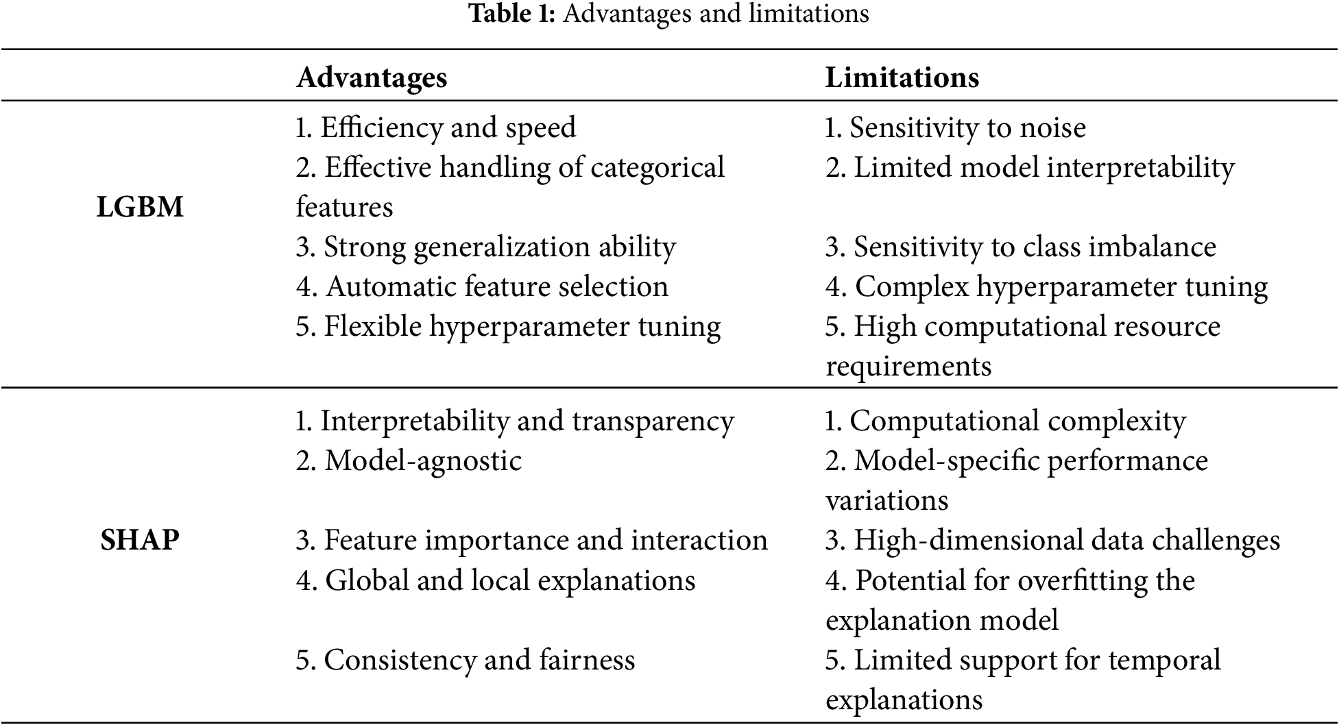
LGBM and SHAP each offer distinct advantages and limitations in network attack prediction. LGBM, with its efficiency and ability to handle large-scale data, enables rapid training and accurate predictions of attacks. It also possesses automatic feature selection and strong generalization capabilities, making it well-suited for various attack patterns. However, LGBM is sensitive to noise, can be affected by class imbalance and high-dimensional features, and suffers from limited interpretability, requiring further tuning. SHAP, as a model-agnostic explainability method, provides clear quantification of each feature’s contribution and reveals feature interactions, offering both global and local explanations that enhance model transparency and trustworthiness. However, SHAP can be computationally expensive, especially with large, high-dimensional datasets, and may struggle to explain temporal data, limiting its ability to offer intuitive and efficient explanations in certain cases.

The structure of this paper is as follows: Section 2 provides an overview of previous literature and related work, Section 3 describes the interpretability method for network attack prediction based on LGBM and SHAP, Section 4 presents the experimental results and analysis, and Section 5 concludes the study.

2  Related Work

The concept of Explainable Artificial Intelligence was first introduced by Van et al. in 2004, initially used to describe their system’s ability to explain the behavior of AI-controlled entities in simulation games. Prior to the introduction of this concept, interpretability issues had emerged as early as the mid-1970s, arising from researchers’ efforts to explain expert systems [22]. However, as artificial intelligence made significant advances in machine learning [23], the pace of research on interpretability slowed. During this period, AI research focused more on model implementation and algorithm performance, particularly predictive capabilities, while less attention was given to explaining the decision-making process.

In recent years, the rapid development and application of large models have made artificial intelligence an essential part of daily life, affecting sensitive areas like security, privacy, and ethics. As a result, there has been increased focus on understanding AI’s decision-making processes in real-world applications, and Explainable Artificial Intelligence has gained significant attention in the academic community. Currently, there is no universally accepted standard or definition for XAI [24]. The concept began to gain broader recognition after DARPA launched the “Explainable AI” project in 2016. Before this, the concept of Interpretable Machine Learning (IML) [25], which overlaps with XAI, had already emerged.

According to DARPA, Explainable Artificial Intelligence refers to AI systems that, while maintaining high performance, produce more interpretable models, helping users understand, trust, and control them better. At the FAT-ML workshop, it was proposed that the goal of interpretability in machine learning is to explain algorithmic decisions and the data behind them to users and stakeholders in simple, non-technical terms. Yeung et al. [26] view XAI as “an innovation for opening the black box of machine learning” and “a challenge in creating models and techniques that are both accurate and capable of providing trustworthy explanations that meet the needs of customers.” These different perspectives on AI interpretability arise from the varying core concerns of different research fields.

From the audience’s perspective, XAI can be defined as a technology that provides details and reasons to make a model simple and clear to understand for specific users [27]. Broadly speaking, XAI technologies encompass all techniques that help developers or users understand the behavior of AI models [28], including both the inherent interpretability of the model and the need for post-hoc explanations. From the perspective of the beneficiaries of intelligent decision-making, AI interpretability refers to methods that clearly explain the rationale behind decisions in a way that can be tailored to users with varying levels of expertise. The goal is to transform the black-box decision-making process of AI into interpretable decision inferences, enabling users to understand and trust the decisions made.

The Mahbooba team [29] explored the use of decision tree models in the IDS (Intrusion Detection System) field to realize the concept of XAI. By building simple decision tree models, they achieved IDS functionality, using threshold values at each node to derive classification rules and rank feature values. The innovation of their work lies in the deeper analysis of the specific rules involved in decision tree classification. In the paper [30], the authors proposed an explanation system based on the SHAP concept to address the interpretability issue in network attack prediction. The researchers first built two deep neural networks on the NSL-KDD network attack dataset and used SHAP to explain the models, gaining insights into the rules used for classification. The main contribution of this research team was the first application of the SHAP explanation model to the intrusion detection field, laying a foundation for future research. Additionally, Liu’s research team [31] introduced a framework called FAIXID, which uses XAI and data cleaning methods to enhance the interpretability and comprehensibility of intrusion detection alerts, helping network analysts make more informed decisions when an alert is triggered. The significant contribution of this study was its attempt to build an explanation evaluation module and quantify the likelihood of a model being explainable.

Currently, there is limited research on the interpretability of AI-based network attack prediction. However, given the security, importance, and reliability of the network attack prediction task, such research is crucial. It is also highly significant for advancing the application of AI in the field of network attack prediction. To address this, this paper conducts an interpretability study on AI-based network attack prediction and proposes an interpretability method based on LGBM [32] and SHAP [33]. The statistical analysis demonstrates that AI-based network attack prediction possesses interpretability.

3  The Interpretability Method for Network Attack Prediction Based on LGBM and SHAP

3.1 Model Description

In network attack prediction, real-time data stream analysis is primarily used to monitor and analyze network traffic data in real-time. Network traffic data includes information such as source IP address, destination IP address, source port number, destination port number, and transmission protocol. By analyzing the data, features related to network attacks can be extracted and further predictions can be made. The process of real-time data stream analysis involves three main steps: data preparation, model training, and SHAP analysis, as shown in Fig. 1. First, during the data preparation stage, network traffic data is collected using tools such as network traffic monitoring devices or sensors. The collected data is then cleaned to remove noise and outliers, followed by appropriate format conversion. Next, during the model training phase, the LGBM model is trained using the processed dataset. Finally, the SHAP algorithm is applied to analyze the data, predict network attack behaviors, and generate an interpretability report, which is then used to inform defense strategies in the prediction model.

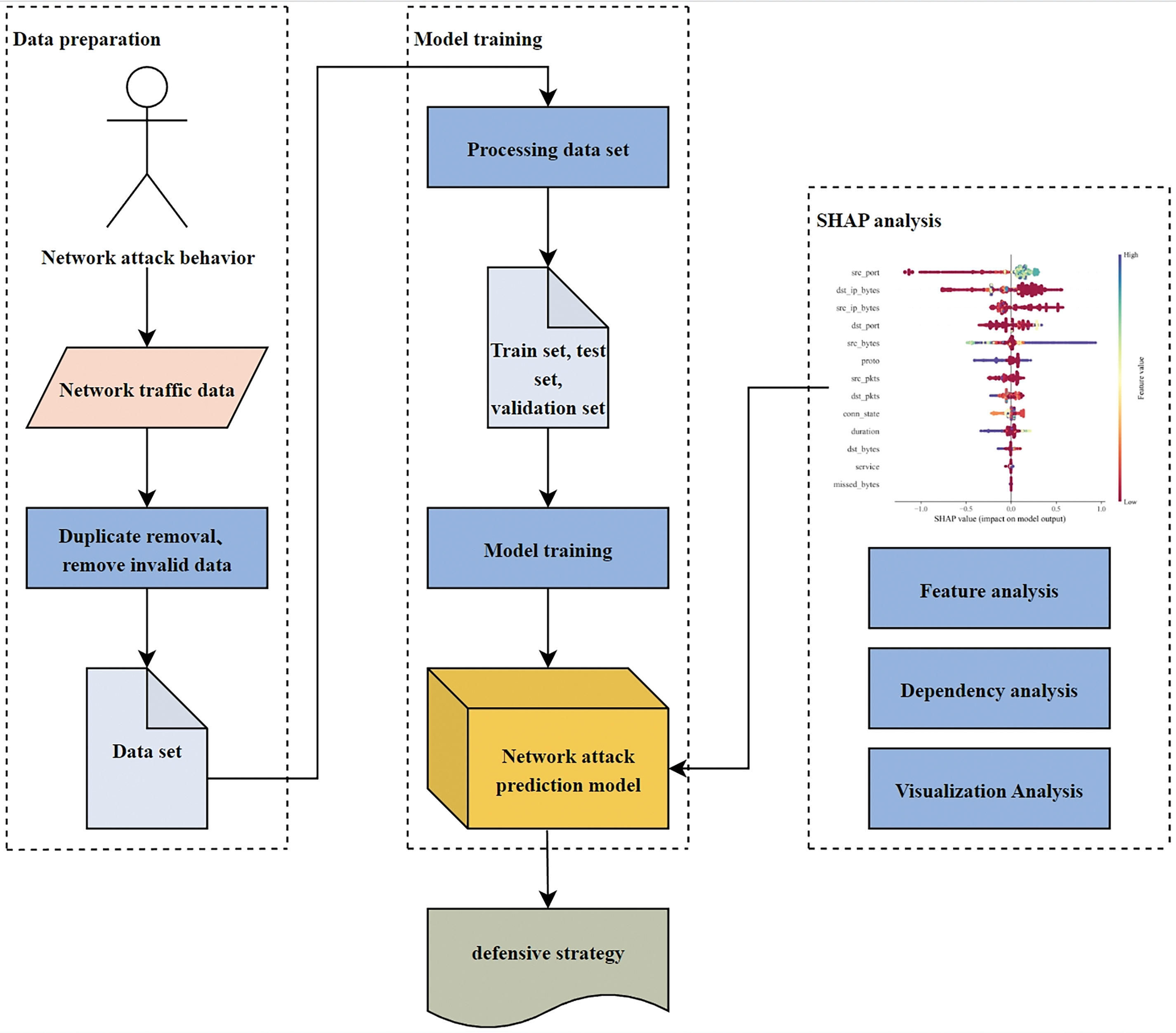
Figure 1: Model flowchart

3.2 LGBM Prediction Model

This paper selects the LGBM model for network attack prediction due to its efficient computation on large datasets, as it is an engineered version of the Gradient Boosting Decision Tree (GBDT) developed by Microsoft. LGBM has the following key features and advantages:

1.    Efficiency: LGBM is a histogram-based algorithm that uses histogram techniques to reduce memory usage and computational costs during the training process. This makes it extremely fast on large-scale datasets and enables it to handle large datasets even with limited memory.

2.    Parallelization: LGBM supports parallel training, effectively utilizing multi-core processors and distributed computing resources, thereby accelerating the training process.

3.    Handling High-Dimensional Features: LGBM can efficiently handle features in high-dimensional spaces.

4.    Accuracy: LGBM improves model accuracy by using a technique called Exclusive Feature Bundling (EFB) to reduce correlations between features.

5.    Sparse Feature Support: LGBM offers strong support for sparse data and can effectively handle features with many zero values.

6.    Scalability: LGBM can be used in conjunction with distributed computing frameworks to achieve training and prediction on large-scale clusters.

The LGBM model can be understood as a comprehensive application of XGBoost, histogram algorithms, Gradient-based One-Side Sampling (GOSS) algorithm, and Exclusive Feature Bundling (EFB) algorithm. The roles of these algorithms are as follows:

1.    Histogram Algorithm: The histogram algorithm reduces the number of candidate split points, optimizing the computation by grouping feature values into discrete bins, which speeds up the training process.

2.    GOSS Algorithm: GOSS reduces the number of samples by focusing on those with larger gradients, thus preserving important information while reducing the computational load. This helps in speeding up the model training by selecting a subset of samples for more efficient gradient calculation.

3.    EFB Algorithm: EFB reduces the number of features by grouping mutually exclusive features. This reduces feature dimensions while maintaining the model’s predictive power, further enhancing training efficiency and accuracy.

3.2.1 Histogram Algorithm

The most time-consuming part of GBDT-based algorithms is finding the optimal split point. To address this issue, XGBoost’s solution is to pre-sort the feature values, which undoubtedly results in a large computational cost and requires significant memory. In contrast, LGBM discretizes continuous features into different bins, where each bin stores gradient statistics. During training, histograms are constructed, reducing the number of feature values that need to be evaluated. Additionally, since the histograms are stored in memory instead of individual feature values, it helps lower memory consumption, as shown in Fig. 2.

Figure 2: Histogram acquisition process

The pseudocode for the histogram algorithm is as follows (Algorithm 1):

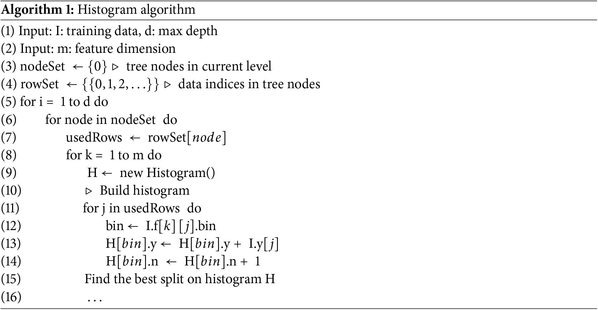
The histogram algorithm can reduce memory consumption by 8 times compared to the pre-sorting algorithm. The pre-sorting algorithm requires storage for feature values (#data∗#feature∗4 Bytes, 32-bit floating-point numbers) and sorted indices (#data∗#feature∗4 Bytes, 32-bit integers). In contrast, the histogram algorithm only needs to store 8-bit histograms (#data∗#feature∗Bytes), directly storing indices in the histogram using bin numbers, without the need for sorting.

When performing node splitting, the histogram of the other child node can be obtained by subtracting the histogram of one child node from the parent node’s histogram. This operation can be performed with a time complexity of O(#bin), achieving acceleration in histogram difference calculation. As shown in Fig. 3.

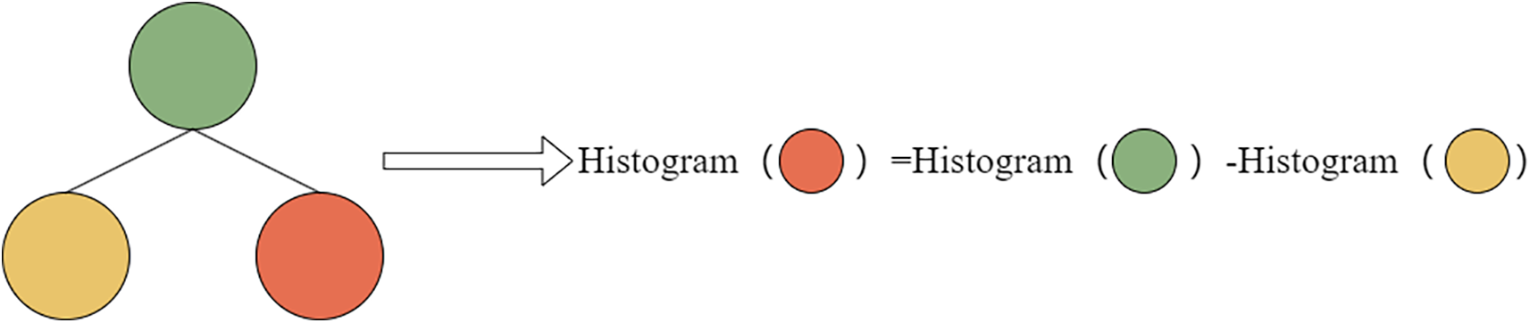
Figure 3: Histogram difference calculation

At the same time, the histogram algorithm used by LGBM is more cache-friendly. First, all features obtain gradients in the same way, and by simply sorting the gradients, continuous access can be achieved, significantly improving cache hit rates. Additionally, there is no need to store an array mapping row indices to leaf indices, which reduces storage consumption and avoids the Cache Miss problem.

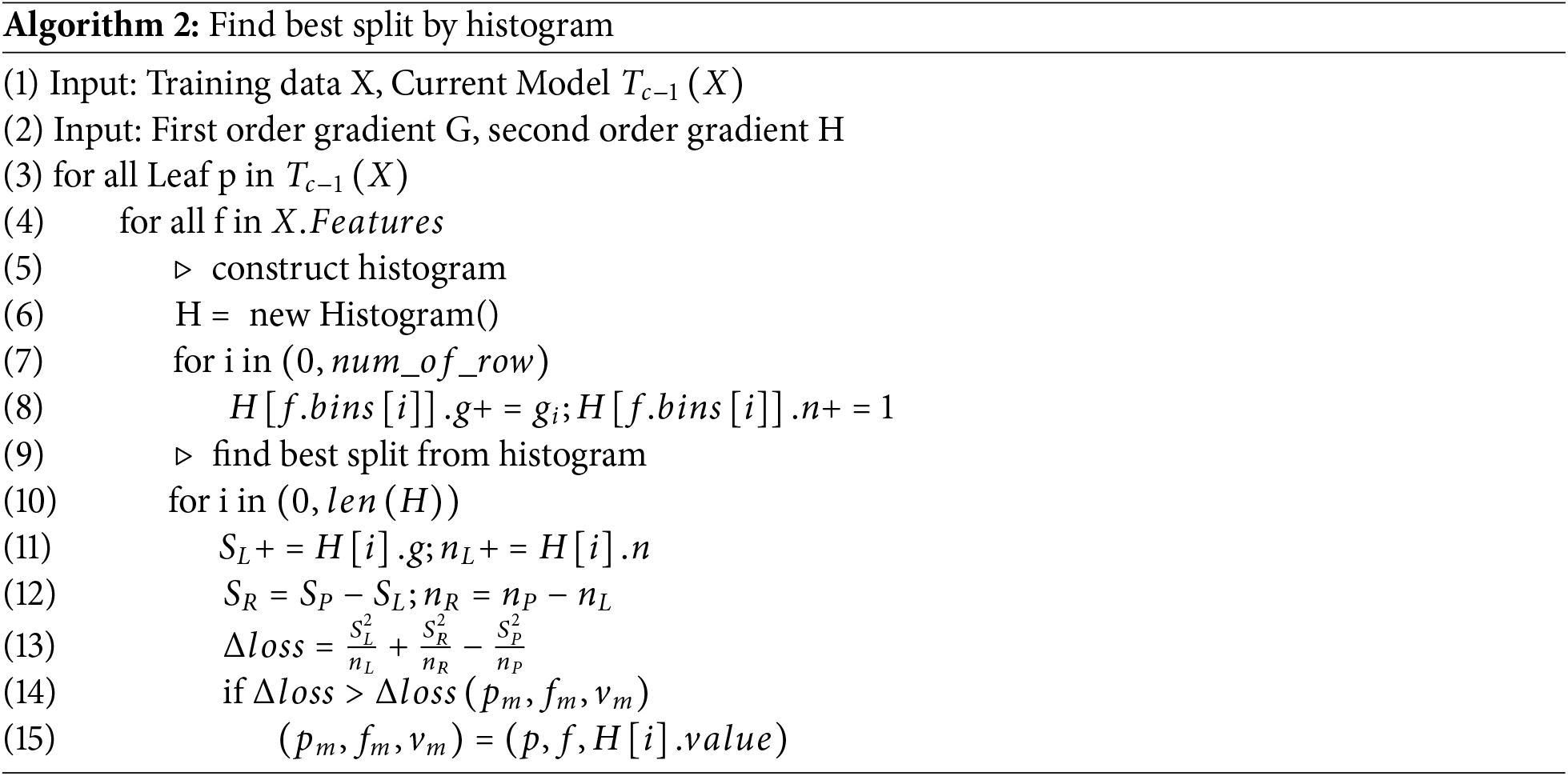
The algorithm for finding the optimal split point using the histogram algorithm is as follows (Algorithm 2):

3.2.2 GOSS Algorithm

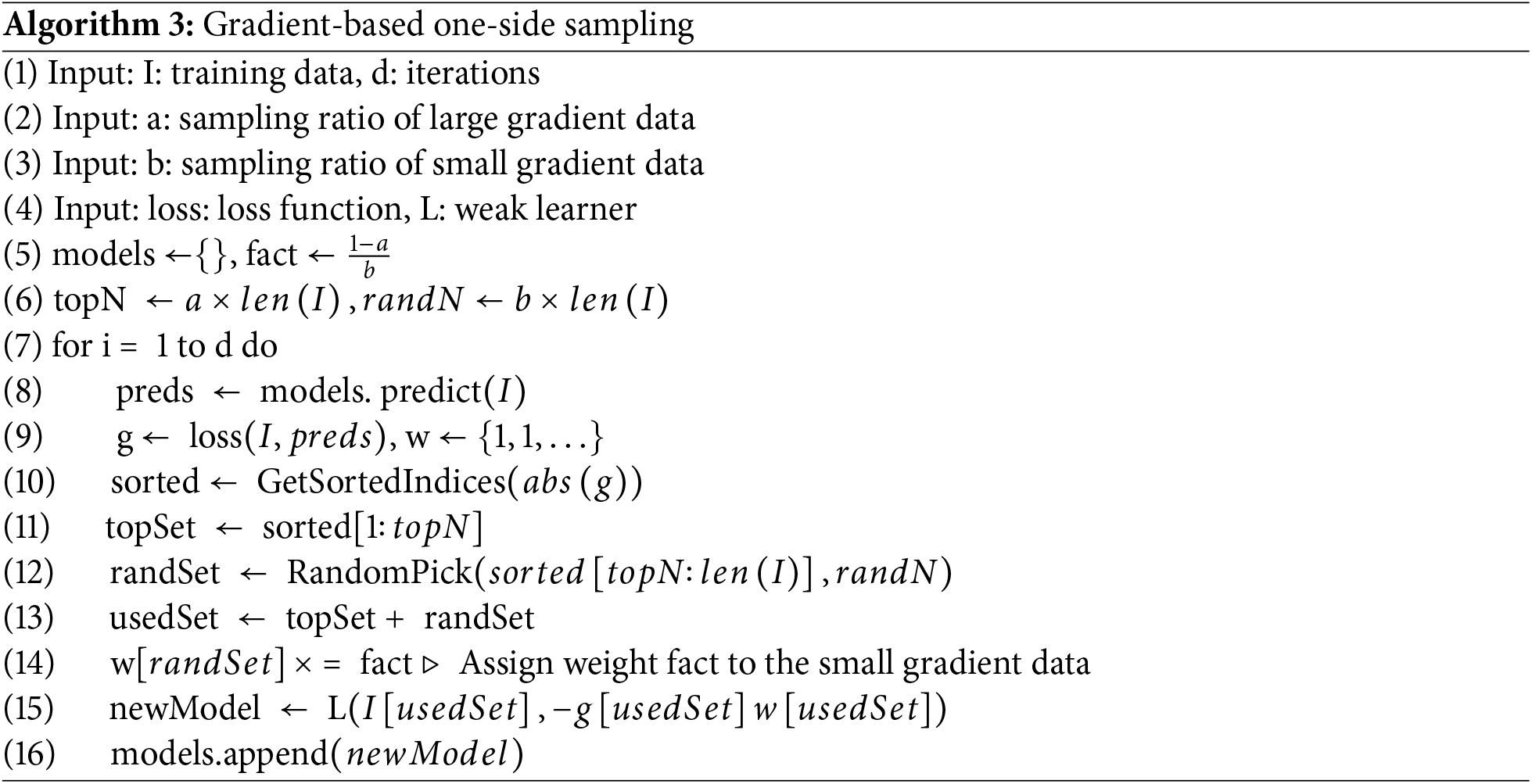
GOSS helps reduce training samples and computational complexity while maintaining the algorithm’s accuracy. GOSS retains all high-gradient samples and randomly selects low-gradient samples for training. To avoid significant changes to the original data distribution, the low-gradient samples are scaled by a factor of 1−ab, where a is the ratio of high-gradient samples selected from the data sorted by gradient, with the top a% set as high-gradient, and b is the proportion of low-gradient samples selected from the remaining data.

The pseudocode for the GOSS algorithm is as follows (Algorithm 3):

The specific implementation process is as follows:

1.    Sort the samples in descending order based on the absolute value of the gradient.

2.    Select the top a × 100% of the samples as the TopSet.

3.    For the remaining (1−a)×100% of the data, randomly sample b×100% of the data to form the RandSet.

4.    Due to the reduced sample set, when calculating the gain, choose to scale the weight corresponding to the RandSet by a factor of 1−ab.

The gain resulting from splitting at point d on feature j, without using the GOSS algorithm, is given by the following formula:

Vj|o(d)=1nO((∑xi∈O:xizdgi)2nl|lOj(d)+(∑xi∈O:xi>dgi)2nr|Oj(d))(1)

where: nO=∑I[xi∈O],nl|Oj(d)=∑I[xi∈O:xij≤d],nr|Oj(d)=∑I[xi∈O:xij>d].

After using the GOSS algorithm, the gain resulting from splitting at point d on feature j becomes:

Vj|o(d)=1nO((∑xi∈Algi+1−ab∑xi∈Blgi)2nlj(d)+(∑xi∈Argi+1−ab∑xi∈Blgr)2nrj(d))(2)

where: Al={xi∈A:xij≤d},Ar={xi∈A:xij>d},Bl={xi∈B:xij≤d},Br={xi∈B:xij>d}, and the coefficient 1−ab is used to normalize the sum of the gradients over B back to the size of Ac. Here, A represents the TopSet, and B represents the RandSet.

The estimation error of GOSS is given by the following formula:

ε(d)≤Ca,b2 ln1δ⋅max{1nlj(d),1nrj(d)}+2DCa,bln1δn(3)

where: Ca,b=1−abmaxxi∈AC|gi|, D=max(g¯lj(d),g¯rj(d)), g¯lj(d)=∑xi∈(A∪AC)l|gi|nlj(d), g¯rj(d)=∑xi∈(A∪AC)r|gi|nrj(d).

This formula shows that the estimation error of GOSS converges within O(n) time complexity. With sufficient data following a globally consistent distribution, the algorithm maintains strong generalization performance.

3.2.3 EFB Algorithm

The principle of the EFB algorithm can be understood as dimensionality reduction, which helps address the issue of high-dimensional sparsity in features. EFB defines feature exclusivity, meaning that features which are never zero simultaneously are considered exclusive. These exclusive features can be merged into a single feature (i.e., a feature bundle), reducing the time complexity of histogram construction from O(#data∗#feature) to O(#data∗#bundle), where #bundle is typically much smaller than #feature.

For feature merging, the solution adopted by LGBM is to transform the problem into a graph coloring problem. This means that, given an undirected graph, the goal is to use as few colors as possible to color each vertex, ensuring that adjacent vertices have different colors. Then, a greedy bundling strategy is used to achieve optimal results. In practical implementation, LGBM allows for a certain proportion of conflicts to compress more features and demonstrates that when the conflict rate (instances where feature values are simultaneously non-zero) is below a certain threshold |γ| (maximum conflict rate), the training accuracy is affected by at most O([(1−γ)n]−23).

The greedy bundling algorithm consists of three steps:

1.    Construct a weighted undirected graph: Nodes represent features, and edges represent the degree of conflict between the nodes.

2.    Sort the graph by degree.

3.    Traverse the sorted nodes: For each node, check whether it satisfies the mutual exclusivity condition with any existing bundle. If it does, add it to that bundle; if not, create a new bundle.

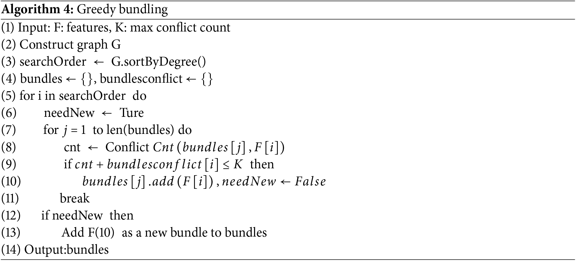
The pseudocode for the greedy bundling algorithm is as follows (Algorithm 4):

The time complexity of this algorithm is O(#feature2). Although it only requires one-time processing before training, the efficiency is still not high when the number of features is large. To address this, LGBM adopts a more efficient sorting strategy by directly sorting features based on the number of non-zero values, which is similar to sorting by degree. This is because a higher number of non-zero values implies a greater likelihood of conflicts.

After selecting the features that need to be merged, the next step is to perform the merging. The key is to ensure that the original features can still be distinguished from the bundles. Since the histogram-based algorithm stores continuous features as discrete bins, it is sufficient to place the mutually exclusive features into different bins. The algorithm’s pseudocode is as follows (Algorithm 5):

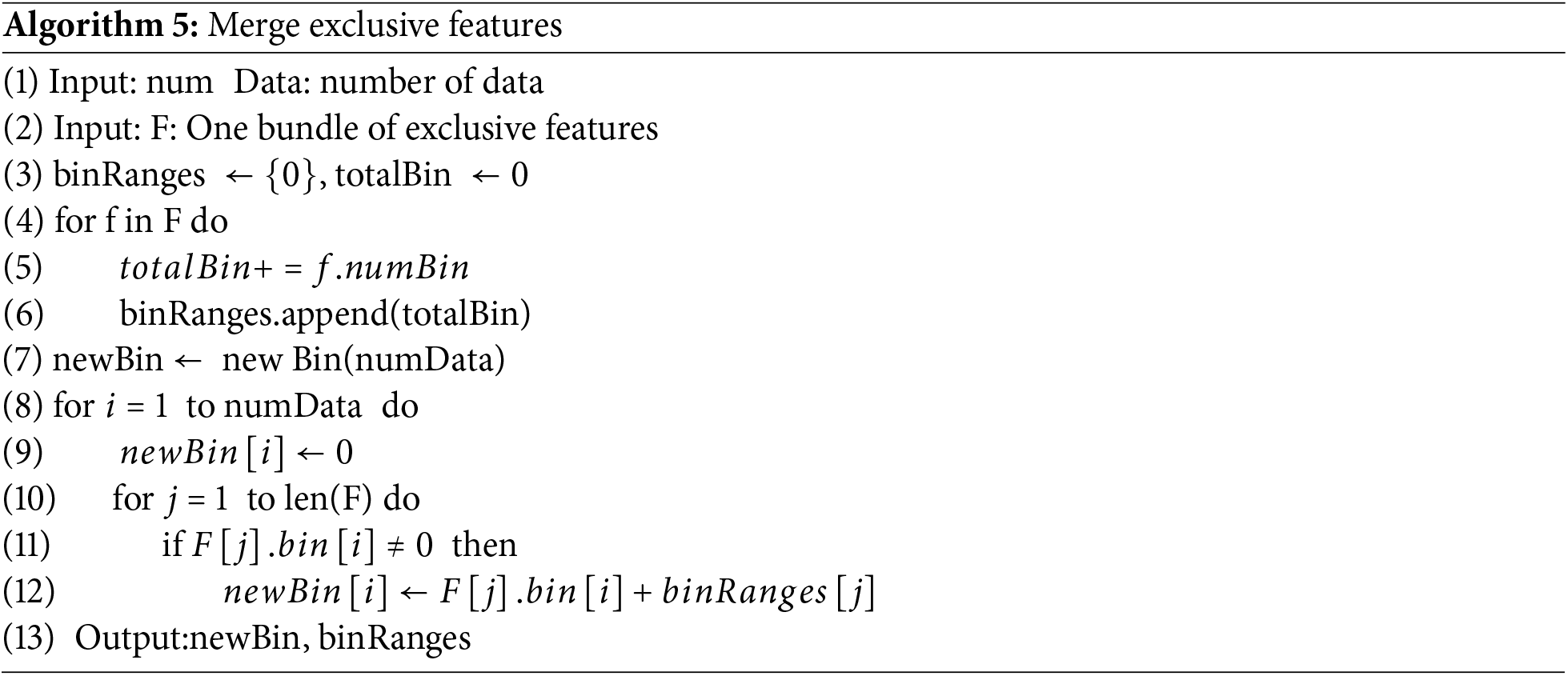
The specific steps are as follows: In the bundle, for the current feature, the number of bins already traversed by all previous features is used as an offset. Then, the bins of all features are merged into a histogram, as shown in Fig. 4.

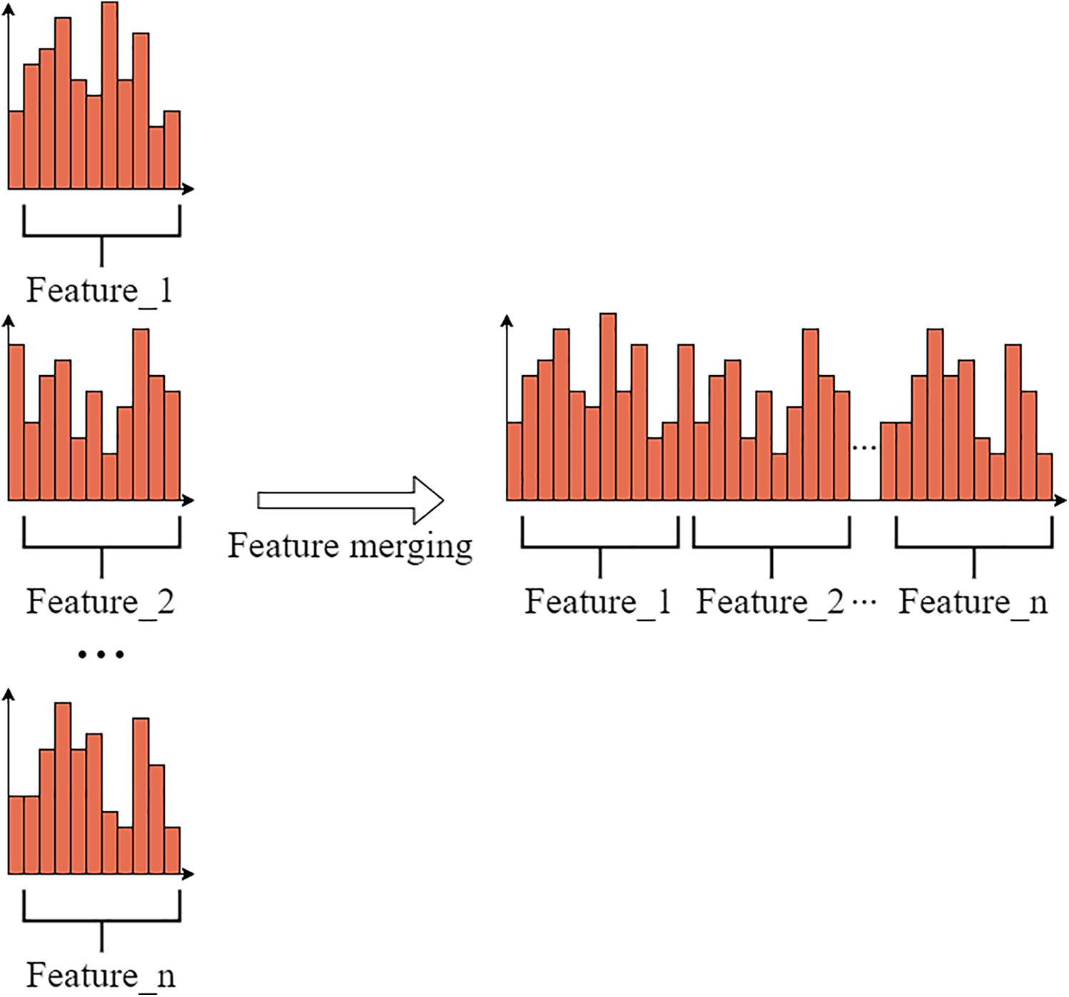
Figure 4: Feature merging diagram

The EFB algorithm can bundle a large number of mutually exclusive features into fewer dense features, effectively avoiding unnecessary computations for zero feature values. At the same time, it can optimize the basic histogram-based algorithm by using a table for each feature to record data with non-zero values, thus ignoring zero feature values. By scanning the data in the table, the cost of constructing the feature histogram is reduced from O(#data) to O(#non_zero_data). However, this approach requires additional memory and computational overhead to maintain a table for each feature during the entire tree-growing process. LGBM integrates this optimization method into a basic function, and it is compatible with EFB because it can still be used when the bundle is sparse.

3.2.4 Optimization of Parallel Learning

LGBM adopts a leaf-wise method for growing trees, which splits nodes in the direction of the highest loss gain. This reduces ineffective splits seen in level-wise growth, but the downside is that it can lead to overfitting, so tree depth must be carefully controlled. While the leaf-wise growth method generates models more quickly and efficiently, it sacrifices some parallelism, whereas the level-wise method is more parallelism-friendly. The comparison between the two is shown in Fig. 5.

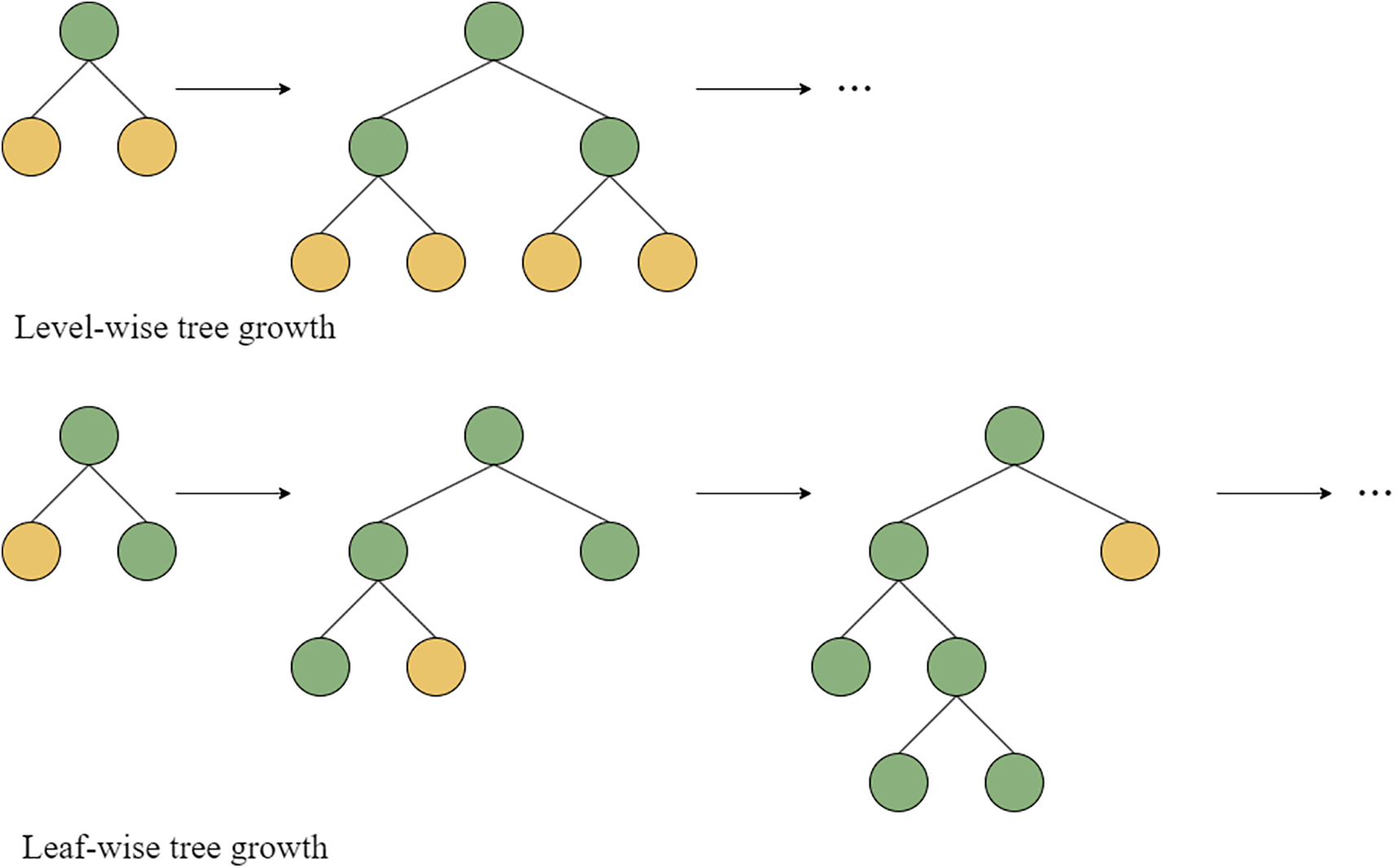
Figure 5: The comparison between leaf-wise and level-wise

LGBM employs three parallel optimization methods: feature parallelism, data parallelism, and voting parallelism.

1.    Feature parallelism mainly targets scenarios with small data and many features. It partitions the data so that all machines have access to the same data samples, but each machine stores a different subset of features. Each machine computes the optimal local split points for its features, and the global optimal split point is determined by aggregating these local results instead of computing it directly. This approach allows efficiency to be improved through distributed computing. As shown in Fig. 6.

2.    Data parallelism mainly targets scenarios with large datasets and fewer features. It partitions the data so that each machine has a subset of the data samples, but each machine contains all features. This way, each machine can construct a local histogram for all features, and then the global histogram for all features can be obtained by combining all the local histograms. Finally, the optimal split point is found based on the global histogram. As shown in Fig. 7.

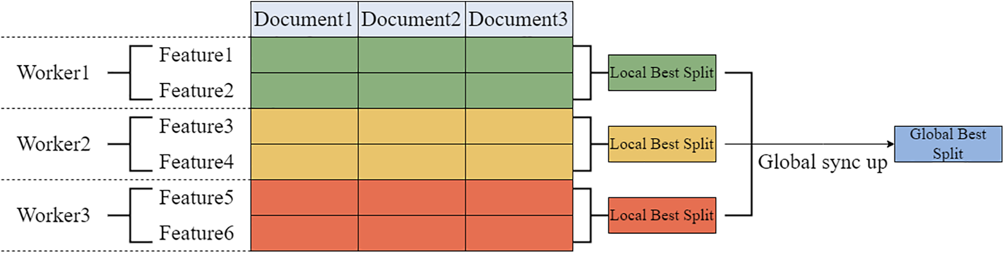
Figure 6: LGBM feature parallelism

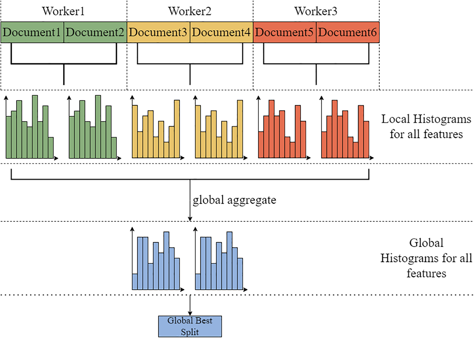
Figure 7: LGBM data parallelism

Voting parallelism mainly targets scenarios with large datasets and many features. It addresses the communication overhead caused by merging feature histograms when using data parallelism. This is done through a two-stage voting process, where only a subset of histograms is merged to mitigate this issue. First, a local voting process is performed to identify the Top k optimal features based on local data. Then, these features are aggregated, and a global vote is conducted to identify the Top 2 ∗ K features most likely to be the global optimal split points. Finally, histograms are merged only for these features. LGBM uses an algorithm called PV-Tree for voting parallelism, which is essentially a form of data parallelism. PV-Tree is similar to a standard decision tree but differs in how the optimal split points are determined. As shown in Fig. 8.

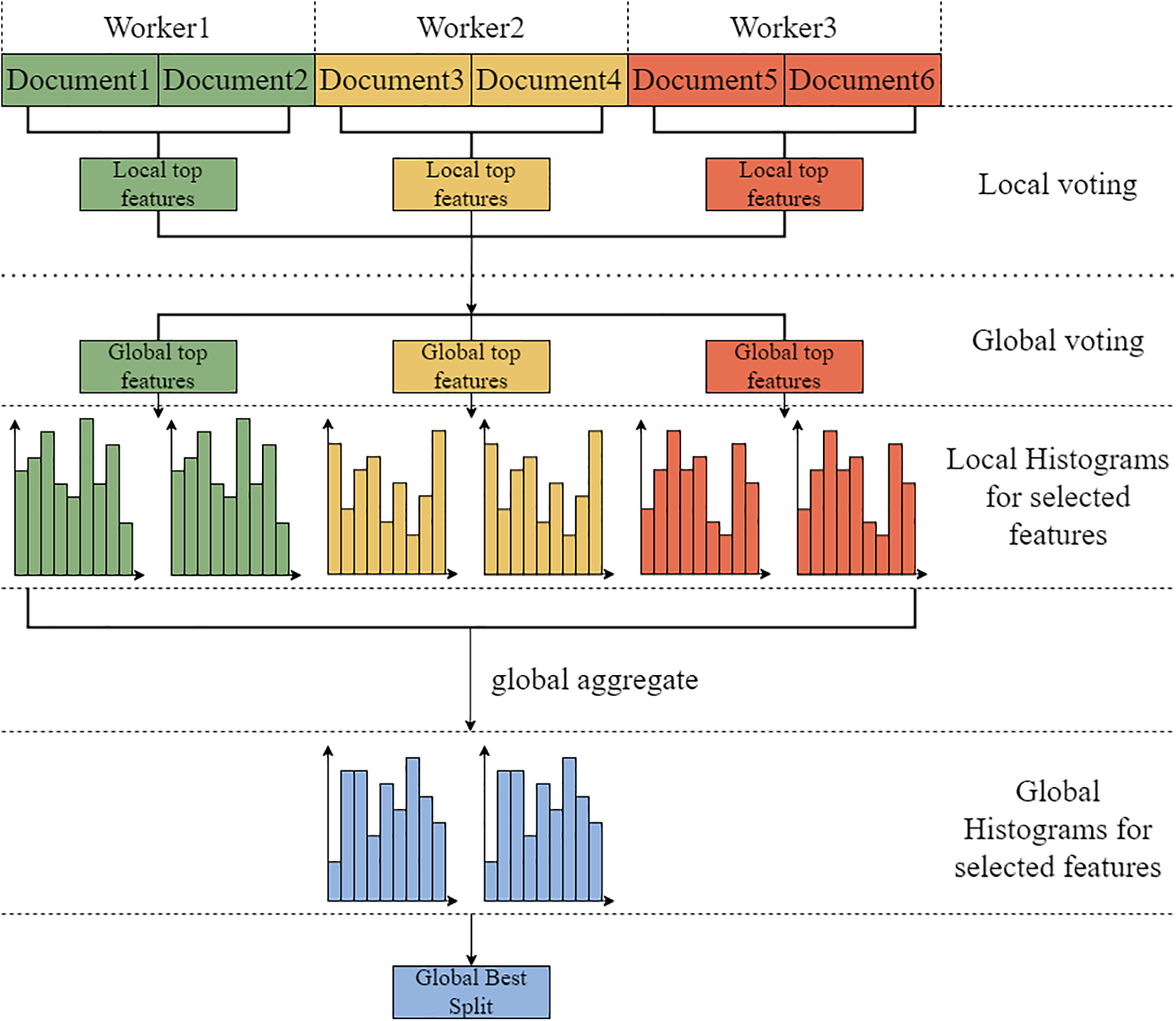
Figure 8: LGBM voting parallelism

LGBM has several advantages, including fast computation speed, low memory consumption, strong capability for handling large-scale data, direct support for categorical feature input, and high interpretability. However, it is sensitive to outliers, requires careful hyperparameter tuning, and may perform less effectively on small datasets compared to XGBoost and Random Forest. XGBoost offers excellent predictive performance, is well-suited for small to medium-sized datasets, and provides strong hyperparameter controllability. However, it has a slower training speed, higher memory consumption, and limited scalability for large datasets compared to LGBM. Random Forest is robust against overfitting, performs well on small datasets, and is resistant to noisy data. However, it suffers from slow training and inference speed, lower model interpretability, and degraded performance in high-dimensional data. Therefore, based on a comprehensive comparison, LGBM is the most suitable choice for the network attack prediction scenario described in this study.

In summary, LGBM is an efficient gradient boosting tree algorithm that offers a scalable and distributed solution, making it well-suited for large-scale datasets and high-dimensional features. The data required for network attack prediction is vast and complex, and using the LGBM model for prediction can significantly improve prediction accuracy and enhance results.

3.3 SHAP Analysis

SHAP (Shapley Additive Explanations) is a method used to explain the prediction results of machine learning models. It is based on Shapley values [34] from cooperative game theory and its extensions, combining optimal credit allocation with local explanations. SHAP offers a unified framework for model interpretability, using SHAP values to fairly quantify each feature’s contribution to predictions. A SHAP value closer to zero indicates a smaller feature contribution, while a value farther from zero signifies a greater impact on the prediction.

SHAP values evaluate the impact of a feature on the prediction result by calculating the average marginal contribution of that feature when it is added to all possible subsets. This average marginal contribution is used as the SHAP value output for that feature. SHAP values have the advantages of fairness, consistency, and model-agnostic properties. SHAP interprets Shapley values as an additive feature attribution method, where the model’s prediction is explained as the sum of the attribution values of each input feature:

g(z′)=ϕ0+∑j=1Mϕjzj′(4)

the formula applies to unstructured data, where g is the explanatory model, and z′∈{0,1}M indicates whether the corresponding feature can be observed (represented by 1 or 0). For structured data, each instance’s features are always observable, even if some are missing—missing features still count as observable information. M represents the number of input features, ϕi∈R is the attribution value (Shapley value) for each feature, and ϕ0 is the constant of the explanatory model, i.e., the mean prediction across all training samples. For structured data, where all features are observable, the formula can be simplified as follows:

g(x′)=ϕ0+∑j=1Mϕj(5)

The calculation process of SHAP is as follows:

1.    Generate all possible feature combinations: Calculate the contribution of each feature in various combinations.

2.    Calculate marginal contribution: For each feature, compute its marginal contribution across different feature combinations.

3.    Calculate the average: Perform a weighted average of the marginal contributions to obtain the SHAP value for the feature.

SHAP has the following characteristics:

1.    Consistency: If a model change results in an increase or no change in the marginal contribution of a feature, the attribution value will also increase or remain unchanged.

2.    Local accuracy: The sum of feature attributions equals the model’s output that needs to be explained. For each instance, the sum of the feature attribution values plus the constant attribution value equals the model’s output value f(x).

f(x)=g(x′)=ϕ0+∑j=1Mϕjxj′(6)

3.    Missingness: A feature xj′=0 has no attribution effect if it is missing. Missingness means that the attribution value for a missing feature is zero. Here, “missing” does not refer to a feature value being empty in structured data, but rather to a feature being unobserved in a given instance. For a structured data instance, all xj′’s are considered as 1, meaning they are observed.

xj′=0→ϕj=0(7)

SHAP has the following functions:

1.    Feature Importance Ranking: SHAP values provide a clear view of which features have the greatest impact on the model’s predictions, allowing for an intuitive ranking of feature importance.

2.    Explaining Individual Predictions: SHAP values can explain the prediction for a single data point, helping to understand why the model made a particular prediction.

3.    Anomaly Detection: By analyzing SHAP values, outliers and potentially problematic features can be identified, which helps in detecting anomalies in the data.

When a model is modified to rely more heavily on a certain feature, the attribution importance of that feature should not decrease. This is the definition of consistency. If consistency is violated, increasing a feature’s impact on the model’s output would paradoxically result in a lower attribution for that feature. This inconsistency prevents meaningful comparison of feature attribution across models, as a higher attribution does not necessarily indicate greater model dependence on that feature.

Feature attribution methods can be divided into global and individualized (for specific cases). Global feature importance is computed for the entire dataset, and such attribution methods typically represent feature importance. The comparison of eight attribution methods: Tree SHAP, Saabas, mean (|Tree SHAP|), Gain, split count, permutation, LIME, and PDP is shown in Table 2.

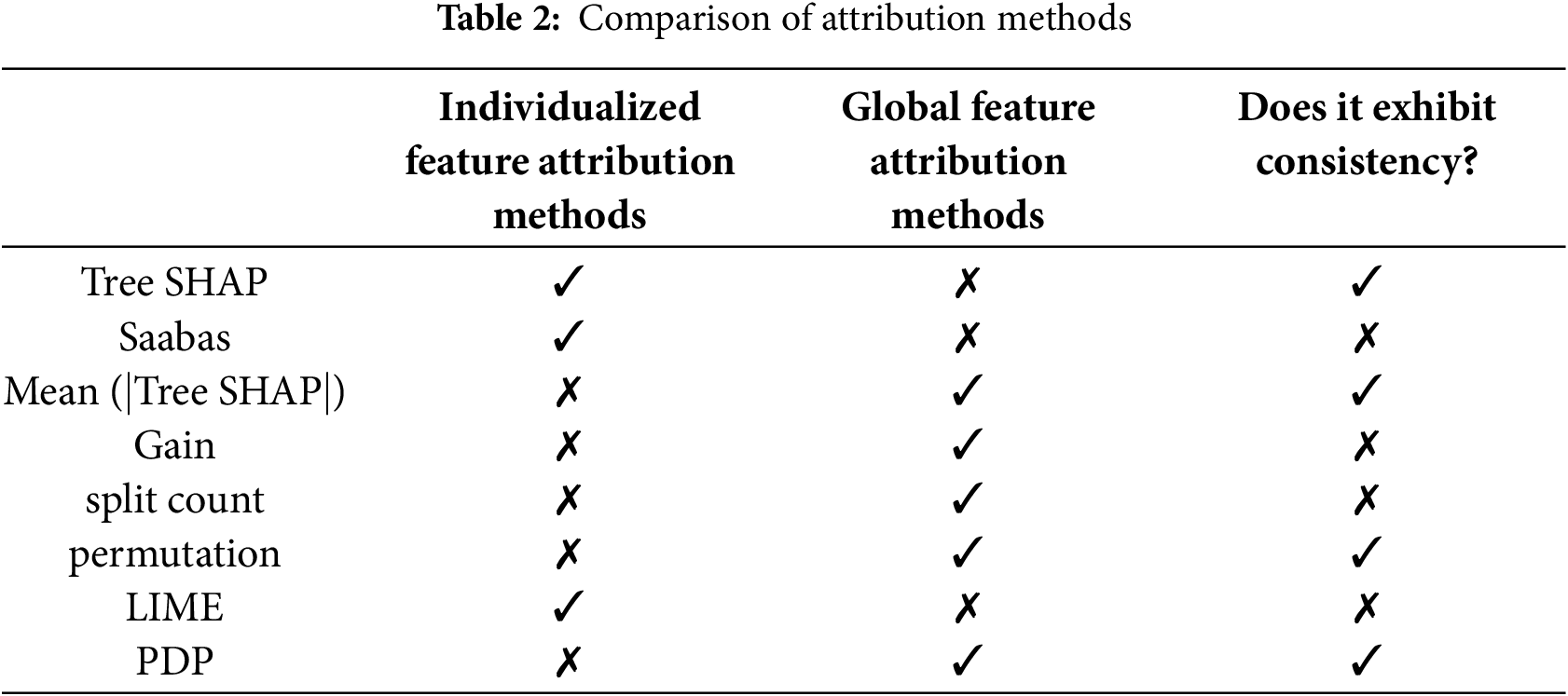
As shown in Table 2, among the eight attribution methods, only SHAP values, permutation, and the PDP method exhibit consistency. However, SHAP values are the only consistent and Individualized attribution method. Furthermore, SHAP enables the visualization of prediction values. Therefore, SHAP is chosen for the interpretability study of the network attack prediction model.

4  Experimental Validation and Analysis

4.1 Experimental Methods and Materials

The hardware configuration for the experiments is as follows: The operating system is Windows 10 64-bit, the CPU is a 12th Gen Intel(R) Core(TM) i7-12700 2.10 GHz, the GPU is an NVIDIA GeForce RTX 3070 Ti, the memory size is 63 GB, ensuring efficient processing and computation of the network attack dataset.

The software environment for the experiments includes PyTorch version 1.12.1 and Python version 3.9. LGBM was selected for training the network attack prediction model, while SHAP was used for the interpretability analysis of the model.

The experimental procedure consists of the following steps: (1) The LGBM model was selected for training the network attack prediction task, and after choosing appropriate hyperparameters, cross-validation was applied for model tuning. (2) SHAP analysis was performed to calculate the contribution of each feature to the model’s output, revealing the decision-making process behind the model’s predictions. (3) The results of the interpretability analysis were visualized to intuitively display feature importance, feature interactions, and other insights, aiding researchers in gaining a deeper understanding of the model.

To enhance numerical stability and computational accuracy, data normalization and standardization were applied to the LGBM model, reducing the impact of feature scale differences on performance. For potential numerical errors in SHAP analysis, the results were averaged over multiple experiments to reduce the influence of random errors.

4.2 Data Overview

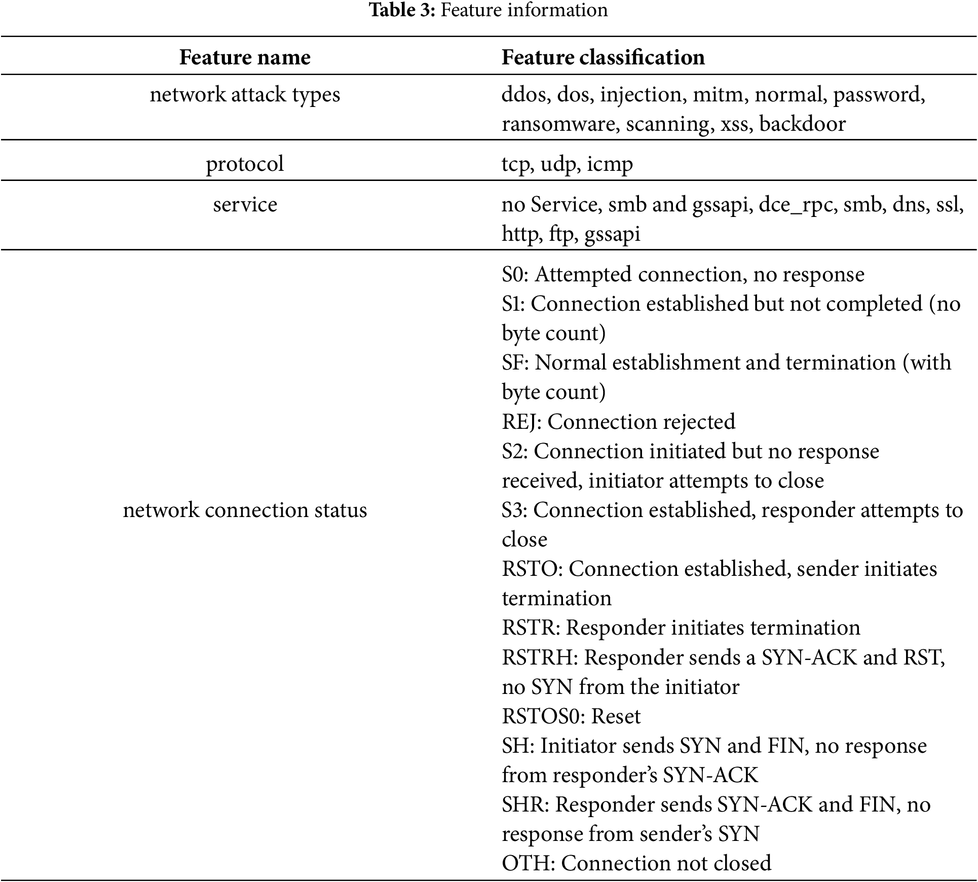
The data in this paper primarily comes from a network attack dataset, which records the status of the attacked host and changes in various network indicators during a network attack. The dataset originates from the logs of hosts that have suffered real network attacks [35]. To improve the training efficiency and accuracy of the model, the following preprocessing steps were applied to the dataset: 1. Handling Missing Data: Missing values in the dataset were imputed using the zero imputation method. This approach ensured the completeness of the dataset and prevented interruptions in model training due to missing data. After analysis, it was determined that imputing missing values with zeros did not significantly affect the prediction results, making it a suitable choice for handling missing data in this study. 2. Outlier Detection and Removal: Manual screening was employed to identify and remove outliers in the dataset. Outliers, which deviate significantly from other data points, may cause bias or instability in the model. Consequently, these outliers were removed to ensure stable training and accurate model predictions. 3. Feature Selection and Removal of Irrelevant Features: Some features in the dataset, particularly those with a large number of missing values, were found to have minimal impact on the prediction results. Therefore, to reduce redundancy and improve model training efficiency, these irrelevant features were removed. After the above preprocessing steps, 13 relevant features were selected for predicting network attack types. These 13 features include the source port number, destination port number, protocol, service, duration, bytes sent by the source, bytes received by the destination, network connection status, unsuccessful data bytes received, number of packets sent by the source, bytes sent by the source IP, number of packets at the destination, and bytes received by the destination IP. The relevant information is shown in Table 3.

The dataset selected for the experiment contains 211,042 network attack records, including 20,000 pieces of DDoS data, 20,000 pieces of DOS data, 20,000 pieces of injection data, 1042 pieces of Mitm data, 50,000 pieces of normal data, 20,000 pieces of password data, 20,000 pieces of ransomware data, 20,000 pieces of scanning data, 20,000 pieces of XSS data, and 20,000 pieces of backdoor data. The dataset was split into training, testing, and validation sets in a 6:2:2 ratio. Specifically, the training set contains 126,625 records, the testing set contains 42,208 records, and the validation set contains 42,209 records.

4.3 Comparison Experiment

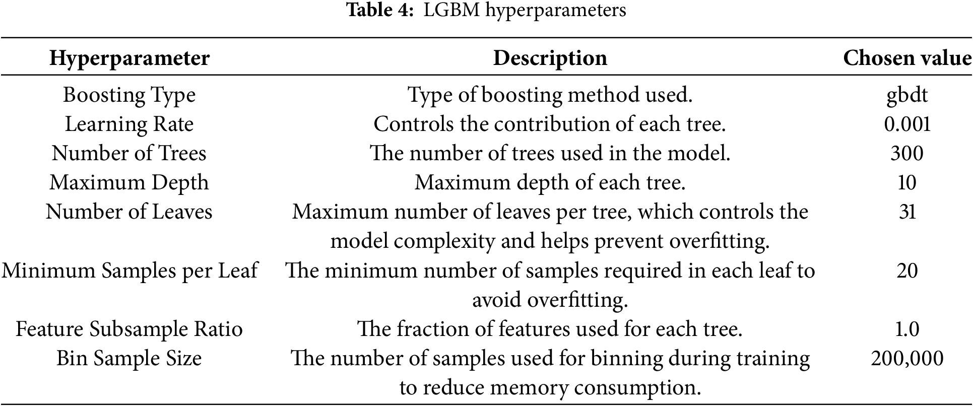
This study uses the LGBM model to build a network attack prediction model. The hyperparameters selected by LGBM are shown in the Table 4.

In the experiment, we also compared the performance of LGBM with four other models, including XGBoost, GBR, CatBoost, and Random Forest. Table 5 presents the performance metrics of the LGBM model compared with four other models after the experimental evaluation.

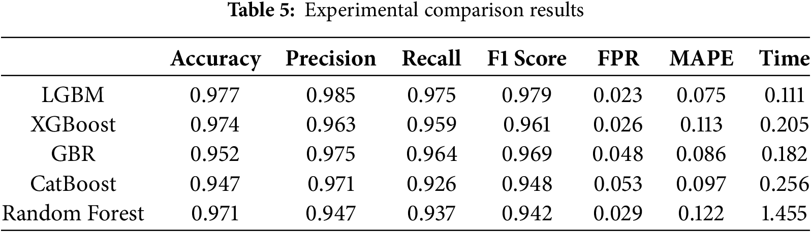
As shown in the table above, the LGBM model outperforms the other models across multiple evaluation metrics, including higher accuracy, precision, recall, F1 score, lower false positive rate, smaller prediction error, and faster runtime. These results indicate that LGBM is more effective in the domain of network attack prediction.

The 95% confidence intervals for the performance metrics of the LGBM model are as follows: Accuracy [0.9756, 0.9784], Precision [0.9838, 0.9862], Recall [0.9735, 0.9765], F1 [0.9785, 0.9795], and FPR [0.0225, 0.0235].

To evaluate the predictive accuracy of the LGBM model compared to other models, we performed the Diebold-Mariano (DM) test. The DM test is designed to compare the forecasting accuracy of two models, with the null hypothesis stating that the models have the same predictive performance, and the alternative hypothesis suggesting significant differences in their predictive accuracy. The results of the DM test indicate that, at the 5% significance level, the null hypothesis cannot be rejected, as the p-values for all models are greater than 0.05. This suggests that there is no significant difference in the predictive accuracy between these models. However, further analysis of the individual error terms reveals that under the experimental conditions, LGBM performs better than the other models. The error boxplots for each model are shown in Fig. 9.

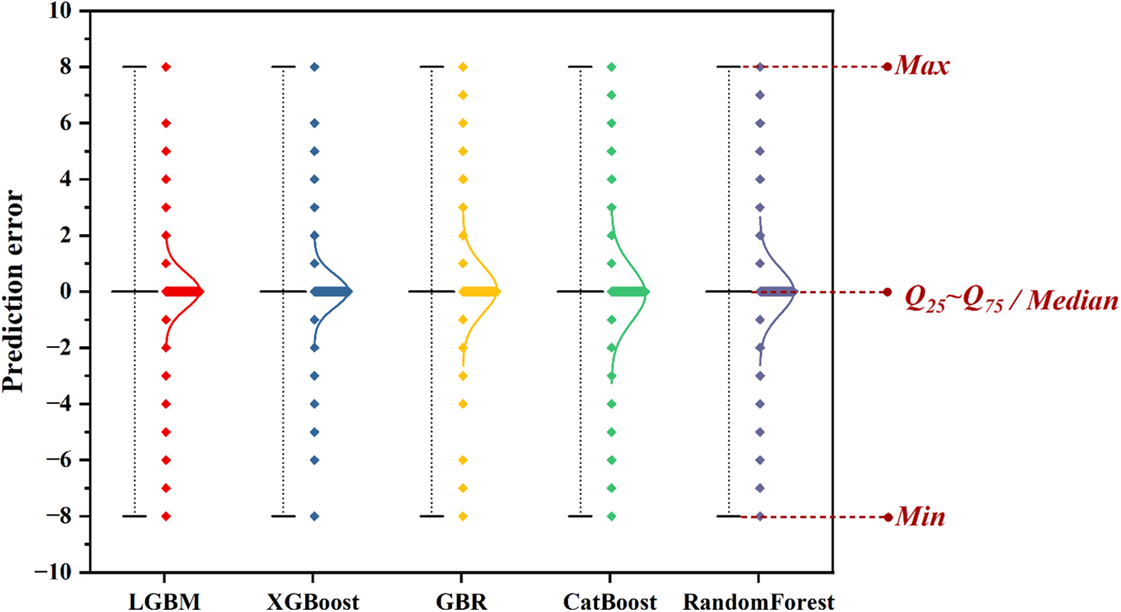
Figure 9: Error boxplot

As shown in Fig. 9, the accuracy and precision of all models are high, with small errors and a relatively dense distribution. Among them, LGBM and XGBoost outperform the other models, which aligns with the metrics presented in Table 5. Combining the information from Table 5, it can be concluded that LGBM has a clear advantage in network attack prediction.

Overall, in the network attack prediction problem, the LGBM model performs better, demonstrating a more accurate ability to predict network attack types. Choosing the LGBM model can effectively improve the defense side’s response to the risk levels of network attacks, helping them formulate and select the most appropriate defense strategies.

4.4 SHAP Experiment Results and Analysis

In this experiment, a network attack prediction model based on LGBM and SHAP was employed, and its prediction results were visualized to provide deeper insights into the model’s interpretability. This visualization enables researchers to better understand the impact of various features on the prediction outcomes. For the visualization, 1000 data samples were selected, where red indicates a positive correlation and blue indicates a negative correlation. The results are presented in Fig. 10, offering a clearer and more comprehensive understanding of the feature contributions to the model’s decisions.

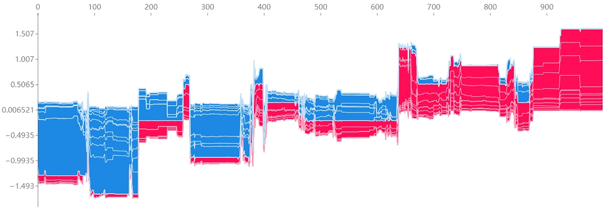
Figure 10: Visualization of 1000 selected data samples based on similarity ranking, highlighting the correlation between various features and the model’s prediction results

For the prediction results, we utilized a SHAP value swarm plot for each feature to assess the impact of individual features on the prediction output from the validation dataset, as shown in Fig. 11. In Fig. 11, the features are ranked based on the total sum of their SHAP values across all samples. The features are arranged in descending order of their influence on the prediction results, with the most influential features positioned at the top and the least influential at the bottom.

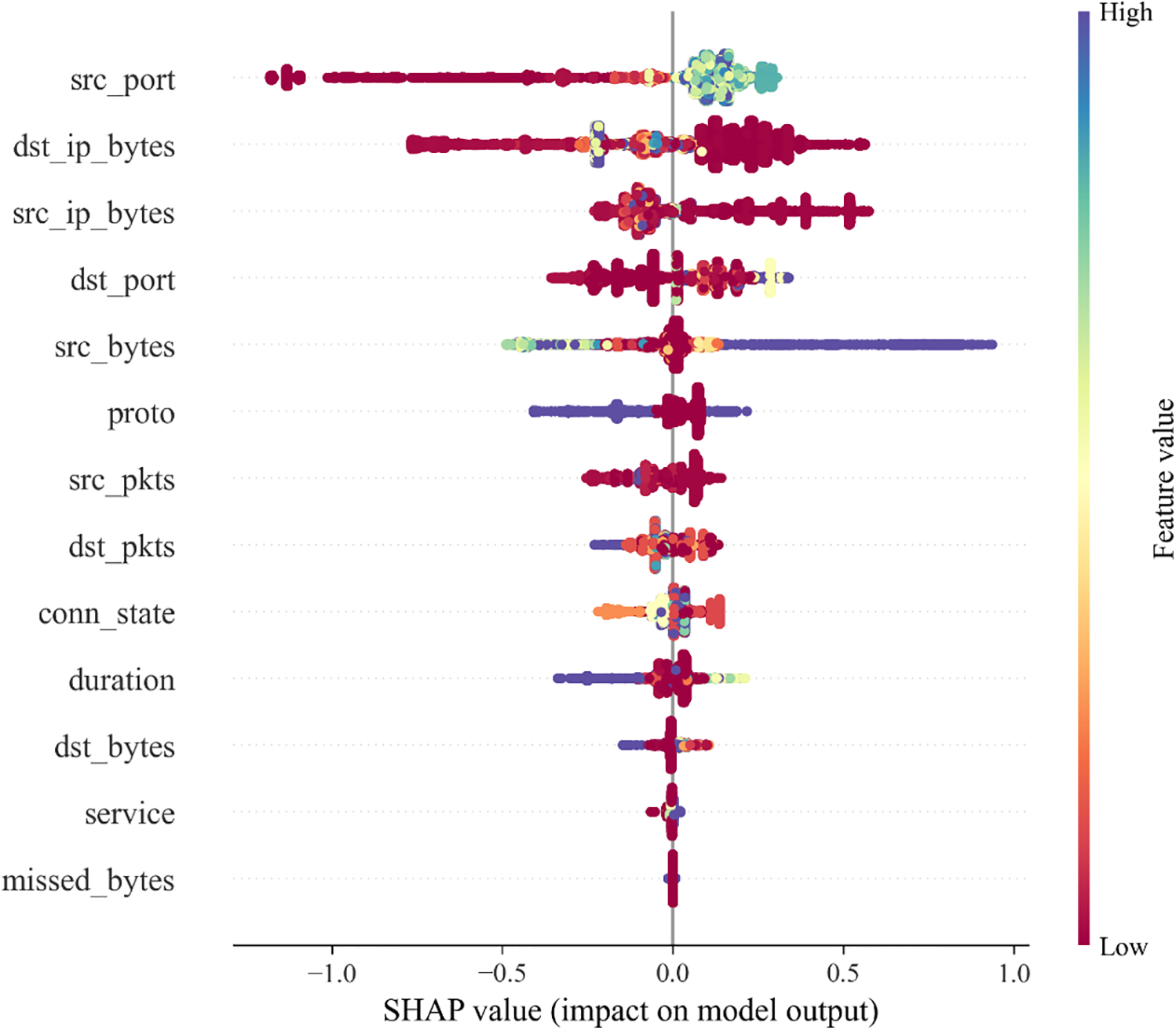
Figure 11: SHAP value swarm plot for each feature, illustrating the impact of each feature on the model’s prediction results, with features ranked by their total SHAP value contributions

From Fig. 11, it can be observed that the features src_port, dst_ip_bytes, src_ip_bytes, dst_port, and src_bytes exert a significant influence on the prediction results. In contrast, features such as proto, src_pkts, dst_pkts, conn_state, and duration show a relatively smaller impact. Furthermore, the features dst_bytes, service, and missed_bytes appear to have minimal effect on the prediction outcomes. Among these features, src_port demonstrates a notable negative impact, while src_bytes has a substantial positive impact on the prediction results.

To provide a more intuitive representation of the impact of each feature on the model’s prediction results, we calculated the average absolute SHAP values for each feature across all predictions and visualized them using a bar chart, as shown in Fig. 12. This approach allows researchers to more easily assess the importance of each feature, offering a clearer interpretation compared to the swarm plot. The results show that src_port has the most significant impact on the prediction outcomes, followed by dst_ip_bytes and src_ip_bytes, while missed_bytes has no discernible effect on the prediction results.

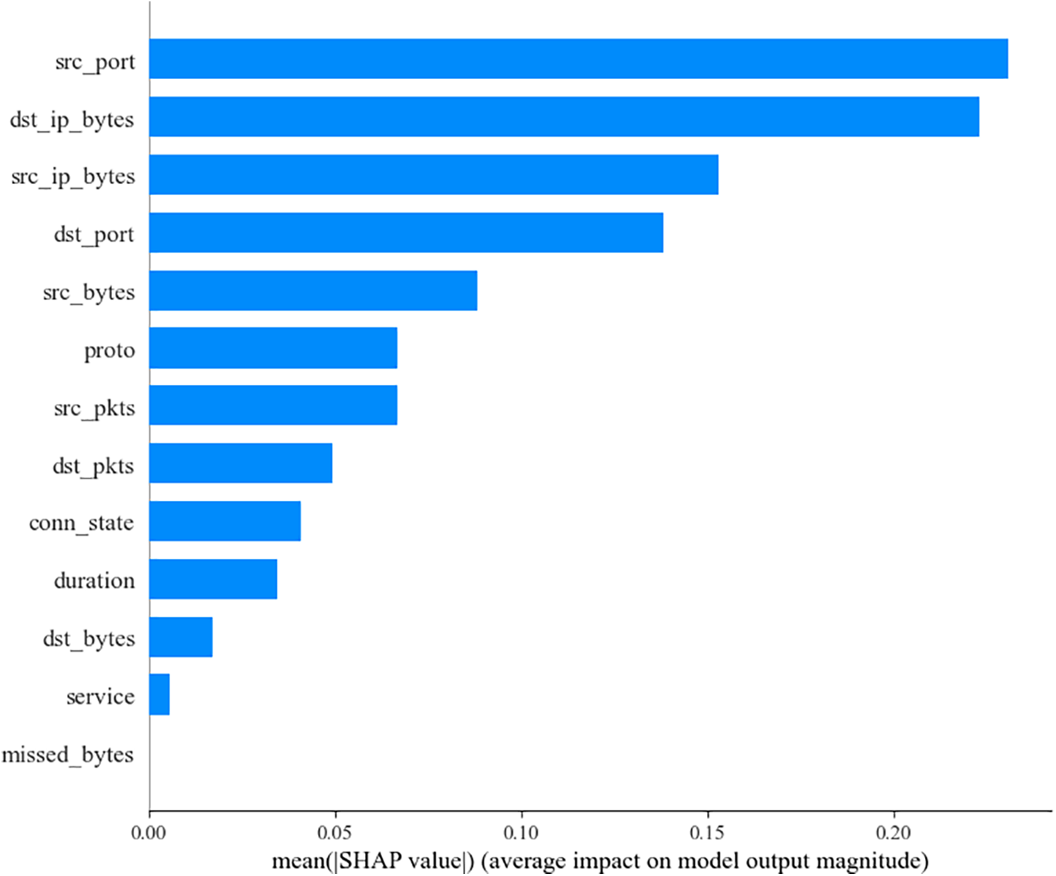
Figure 12: SHAP value average importance bar chart, showing the average contribution of each feature to the model’s prediction results. This chart helps identify the most influential features in the network attack prediction model

The SHAP dependence plot illustrates the impact of an individual feature on the prediction results across the entire dataset, showing the relationship between the feature values and their corresponding SHAP values across multiple samples. It also takes into account interaction effects between features, highlighting potential interactions between pairs of features that could influence the prediction results. Since 13 features were selected for analysis in this experiment, a total of 78 interaction plots were generated between feature pairs. In this paper, we focus on the five most influential features on prediction results: src_port, dst_ip_bytes, src_ip_bytes, dst_port, and src_bytes. We present 10 interaction plots between these features, as shown in Fig. 13. In these plots, the x-axis represents the actual values of the features, the y-axis represents their respective SHAP values, and the color indicates the value of the interacting feature, ranging from low to high. These plots not only reveal the relationship between the feature values and their SHAP values but also allow the influence of other features on the prediction results to be observed through color, offering a clear visual representation of the interaction effects and their combined impact on the model’s prediction.

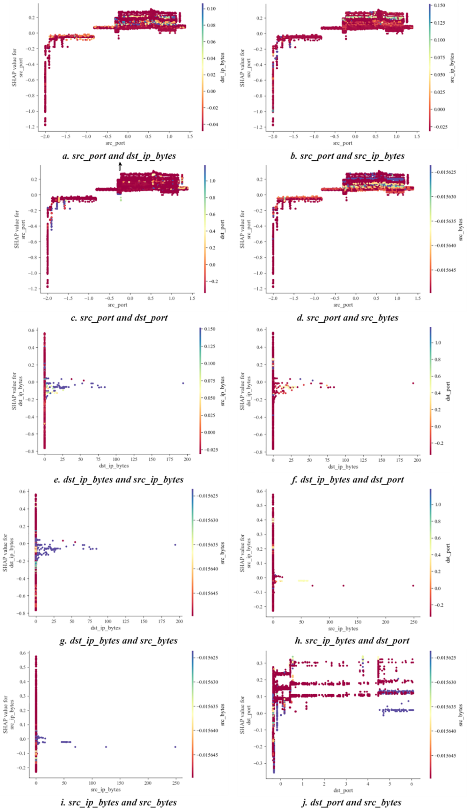
Figure 13: SHAP feature dependence plot between selected features, illustrating the relationship between the feature values and their SHAP values across multiple samples. This plot also shows potential interaction effects between pairs of features

In the experiment, SHAP was employed to generate a force plot, which provides a detailed visualization of the feature contributions for a single prediction. The contribution of each feature to the prediction result is represented by arrows, as shown in Fig. 14. Red arrows indicate a positive contribution, while blue arrows represent a negative contribution. The length of the red arrow indicates the magnitude of the positive impact, and the length of the blue arrow indicates the magnitude of the negative impact. The baseline value in the figure corresponds to the model’s average output, and the prediction result reflects the final outcome after considering the combined effects of all features. This force plot effectively demonstrates the significance and direction of each feature’s influence during the prediction process.

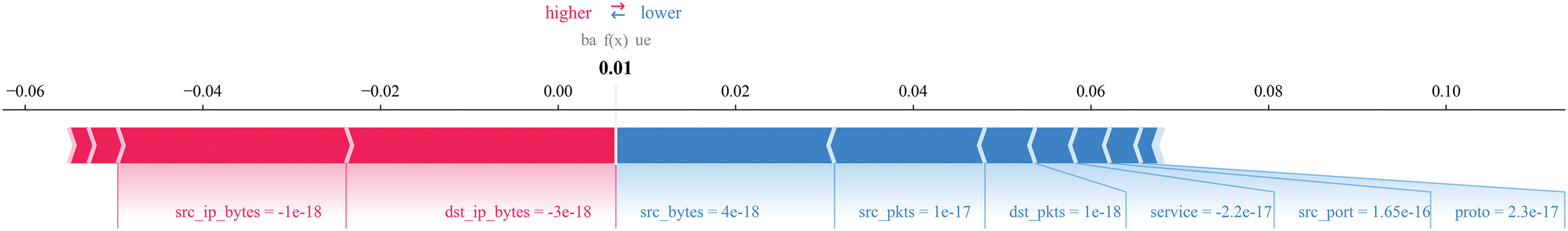
Figure 14: SHAP force plot illustrating the detailed feature contributions for a single prediction. The plot visually demonstrates how each feature impacts the model’s prediction outcome

To more intuitively illustrate the interaction effects between features, this study selected the seven most influential features on the prediction results and utilized SHAP to generate interaction plots between these features, as shown in Fig. 15. The diagonal displays the main effects of each individual feature, while the regions on either side of the diagonal highlight the interactions between pairs of features. The greater the scatter of the points, the stronger the interaction effect between the features.

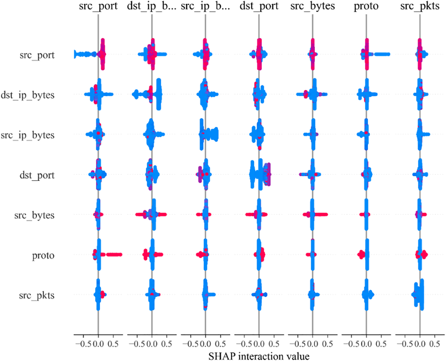
Figure 15: SHAP feature interaction plot showing the interactions between the top 7 most influential features. The diagonal displays the main effects, while the off-diagonal areas highlight the interactions between pairs of features. The scatter of points indicates the strength of the interaction effect

By evenly distributing the points for each feature, rather than arranging them densely as in previous charts, we can obtain a SHAP value heatmap that more aesthetically displays the impact of each feature on the prediction result, as shown in Fig. 16. In this figure, the left y-axis ranks the features by their importance, from smallest to largest, while the right y-axis represents the corresponding visualized results. The red color indicates a positive impact, while blue represents a negative impact. The intensity of the color reflects the magnitude of the SHAP value, representing the influence of the feature value on the model. The deeper the color, the larger the absolute SHAP value and the greater the effect on the model. The top function visualizes the model’s prediction result under these values, i.e., the model’s output. Fig. 16 shows the heatmap visualization of 3000 data points

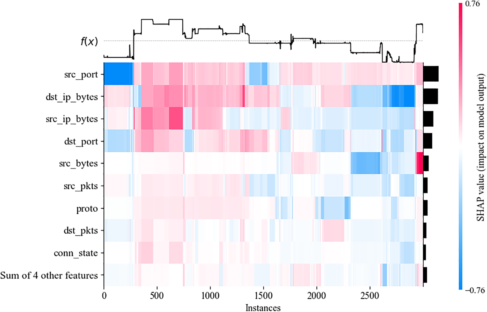
Figure 16: SHAP Heatmap visualizing the impact of features on prediction results

In conclusion, acquiring detailed information about the source of a network attack is essential for effective defense strategies. This information enables defenders to comprehend the attacker’s intentions, predict likely attack methods, and devise appropriate countermeasures to mitigate the security risks associated with network attacks. These findings are consistent with real-world scenarios, where the lack of insight into the adversary makes it challenging to anticipate their attack strategies. As the adage goes, ‘Know yourself, know your enemy, and you will never be defeated’.

By conducting interpretability research on the network attack prediction results of LGBM using SHAP, and visualizing the impact of various features on the model’s predictions, researchers can gain a deeper understanding of the relationships between network features and network attacks. The SHAP visualizations, such as force plots, dependence plots, and feature importance charts, provide intuitive and detailed insights into how each feature contributes to the prediction outcome. The model proposed in this study allows defenders to predict the type of network attack that is most likely to occur based on abnormal changes in network feature indicators. These visual tools enable defenders to easily interpret complex data patterns and take timely, targeted defense strategies, thereby enhancing the overall security of the system.

Although the approach presented in this paper has achieved some promising results, several challenges remain to be addressed. The current method selects only 13 network attack-related features. Incorporating more features could broaden the study’s scope and improve the generalizability of the conclusions. Furthermore, the model requires further improvement in terms of both prediction accuracy and computational speed. We aim to draw inspiration from emerging machine learning and artificial intelligence algorithms. In future work, we plan to enhance the prediction model by incorporating real-time evolving attack data, thereby improving its versatility and practical applicability in the field of cybersecurity. This will not only extend its use to network attack prediction but also aim to boost its overall performance and prediction quality.

In addition, LGBM, as a tree-based gradient boosting model, exhibits certain robustness against traditional gradient-based adversarial attacks. However, it remains vulnerable to feature perturbation and adversarial evasion strategies, where attackers manipulate key input features to deceive the model. Due to its reliance on decision rules, LGBM is sensitive to modifications in highly influential features, which can lead to misclassification. To enhance its robustness in real-world network security applications, several strategies can be employed, including adversarial training, feature selection based on SHAP analysis to reduce reliance on easily manipulated features, and integrating anomaly detection methods to identify adversarial samples. Additionally, ensemble approaches, such as combining LGBM with Random Forest or deep learning models, can further mitigate the impact of adversarial attacks. These enhancements contribute to improving the reliability and security of LGBM-based network attack prediction systems.

5  Conclusion

As network security issues become increasingly prominent, understanding the abnormal changes in various network metrics during a network attack and predicting potential attacks has become an important practice. This helps ensure the security and stability of system operations. In this context, this paper employs the efficient LGBM model to analyze real network attack data and utilizes SHAP analysis to offer a scientific basis for defense decision-making. The paper proposes an interpretability research method for a network attack prediction model based on LGBM and SHAP, incorporating the abnormal changes in 13 feature metrics during a network attack into the prediction analysis. It also compares and discusses the performance of different prediction models. Finally, the paper uses SHAP analysis to visualize the contribution of each feature, with results showing that information about the attack source has a more significant impact on the prediction outcome. Understanding these influencing factors is crucial for formulating effective defense strategies. The proposed method has a certain degree of generalizability when facing other types of network attack prediction problems. The innovation of this study lies in combining LGBM and SHAP, presenting a network attack detection framework that offers both high prediction accuracy and high interpretability. This framework provides a more transparent and reliable solution for the application of artificial intelligence in network security, with significant academic value and practical implications. Future work will focus on further optimizing the model’s performance and exploring more network security defense strategies based on interpretability methods.

Acknowledgement: The authors would like to thank all those who have contributed in this area and the anonymous reviewers for their valuable comments and suggestions, which have improved the presentation of this paper.

Funding Statement: This paper was supported by the National Natural Science Foundation of China Project (No. 62302540), please visit their website at https://www.nsfc.gov.cn/ (accessed on 18 June 2024).

Author Contributions: The authors confirm contribution to the paper as follows: study conception and design: Shuqin Zhang, Zihao Wang; data collection: Xinyu Su; analysis and interpretation of results: Zihao Wang, Xinyu Su; draft manuscript preparation: Zihao Wang. All authors reviewed the results and approved the final version of the manuscript.

Availability of Data and Materials: The code involved in this paper can be obtained by sending an E-mail to the corresponding author.

Ethics Approval: Not applicable.

Conflicts of Interest: The authors declare no conflicts of interest to report regarding the present study.

References

1. Smith RG, Eckroth J. Building AI applications: yesterday, today, and tomorrow. AI Mag. 2017;38(1):6–22. doi:10.1609/aimag.v38i1.2709. [Google Scholar] [CrossRef]

2. Von Eschenbach WJ. Transparency and the black box problem: why we do not trust AI. Philos Technol. 2021;34(4):1607–22. doi:10.1007/s13347-021-00477-0. [Google Scholar] [CrossRef]

3. Pillai V. Enhancing transparency and understanding in AI decision-making processes. Iconic Res Eng J. 2024;8(1):168–72. [Google Scholar]

4. Atakishiyev S, Salameh M, Yao H, Goebel R. Explainable artificial intelligence for autonomous driving: a comprehensive overview and field guide for future research directions. IEEE Access. 2024;12:10163–25. doi:10.1109/ACCESS.2024.3431437. [Google Scholar] [CrossRef]

5. Shaheen MY. Applications of Artificial Intelligence (AI) in healthcare: a review. ScienceOpen Preprints. 2021. doi:10.14293/S2199-1006.1.SOR-.PPVRY8K.v1. [Google Scholar] [CrossRef]

6. van Ettekoven BJ, Prins C. Artificial intelligence and the judiciary system. In: Mark V, Tai ETT, Berlee A, editors. Research handbook in data science and law. 2nd ed. Cheltenham, UK: Edward Elgar Publishing; 2024. p. 361–87. [Google Scholar]

7. An H, Xing Y, Zhang G, Bamisile O, Li J, Huang Q. Cluster partition-fuzzy broad learning-based fast detection and localization framework for false data injection attack in smart distribution networks. Sustain Energy Grids Netw. 2024;40:101534. doi:10.1016/j.segan.2024.101534. [Google Scholar] [CrossRef]

8. Ansari MF, Dash B, Sharma P, Yathiraju N. The impact and limitations of artificial intelligence in cybersecurity: a literature review. Int J Adv Res Comput Commun Eng. 2022;11(9):81–90. doi:10.17148/IJARCCE.2022.11912. [Google Scholar] [CrossRef]

9. Mohale VZ, Obagbuwa IC. A systematic review on the integration of explainable artificial intelligence in intrusion detection systems to enhancing transparency and interpretability in cybersecurity. Front Artif Intell. 2025;8:1526221. doi:10.3389/frai.2025.1526221. [Google Scholar] [PubMed] [CrossRef]

10. Van Lent M, Fisher W, Mancuso M. An explainable artificial intelligence system for small-unit tactical behavior. In: Proceedings of the National Conference on Artificial Intelligence; 2004 Jul 25–29; San Jose, CA, USA. [Google Scholar]

11. Gunning D, Aha D. DARPA’s explainable artificial intelligence (XAI) program. AI Mag. 2019;40(2):44–58. doi:10.1609/aimag.v40i2.2850. [Google Scholar] [CrossRef]

12. Hoque N, Bhuyan MH, Baishya RC, Bhattacharyya DK, Kalita JK. Network attacks: Taxonomy, tools and systems. J Netw Comput Appl. 2014;40:307–24. doi:10.1016/j.jnca.2013.08.001. [Google Scholar] [CrossRef]

13. Abbas NN, Ahmed T, Shah SHU, Omar M, Park HW. Investigating the applications of artificial intelligence in cyber security. Scientometrics. 2019;121:1189–211. doi:10.1007/s11192-019-03222-9. [Google Scholar] [CrossRef]

14. Husák M, Komárková J, Bou-Harb E, Čeleda P. Survey of attack projection, prediction, and forecasting in cyber security. IEEE Commun Surv Tutor. 2018;21(1):640–60. doi:10.1109/COMST.2018.2871866. [Google Scholar] [CrossRef]

15. Charmet F, Tanuwidjaja HC, Ayoubi S, Gimenez PF, Han Y, Jmila H, et al. Explainable artificial intelligence for cybersecurity: a literature survey. Ann Telecommun. 2022;77(11):789–812. doi:10.1007/s12243-022-00926-7. [Google Scholar] [CrossRef]

16. Vaassen B. AI, opacity, and personal autonomy. Philos Technol. 2022;35(4):88. doi:10.1007/s13347-022-00577-5. [Google Scholar] [CrossRef]

17. Sindiramutty SR, Tan CE, Lau SP, Thangaveloo R, Gharib AH, Manchuri AR, et al. Explainable AI for cybersecurity. In: Ghonge MM, Pradeep N, Jhanjhi NZ, editors. Advances in explainable AI applications for smart cities. New York, NY, USA: IGI Global Scientific Publishing; 2024. p. 31–97. [Google Scholar]

18. Lockey S, Gillespie N, Holm D, Someh IA. A review of trust in artificial intelligence: challenges, vulnerabilities and future directions. In: Proceedings of the 54th Hawaii International Conference on System Sciences; 2021 Jan 5; Kauai, HI, USA. [Google Scholar]

19. Wang W, Harrou F, Bouyeddou B, Senouci SM, Sun Y. Cyber-attacks detection in industrial systems using artificial intelligence-driven methods. Int J Crit Infrastruct Prot. 2022;38:100542. doi:10.1016/j.ijcip.2022.100542. [Google Scholar] [CrossRef]

20. Adhikari D, Thapaliya S. Explainable AI for cyber security: interpretable models for malware analysis and network intrusion detection. NPRC J Multidiscip Res. 2024;1(9):170–9. doi:10.3126/nprcjmr.v1i9.74177. [Google Scholar] [CrossRef]

21. Camacho NG. The role of ai in cybersecurity: addressing threats in the digital age. J Artif Intell Gen Sci. 2024;3(1):143–54. doi:10.60087/jaigs.v3i1.75. [Google Scholar] [CrossRef]

22. Alameda-Pineda X, Redi M, Celis E, Sebe N, Chang SF. FAT/MM’19: 1st international workshop on fairness, accountability, and transparency in multimedia. In: Proceedings of the 27th ACM International Conference on Multimedia; 2019 Oct 21–25; Nice, France. [Google Scholar]

23. Guy TV. NIPS Workshop on imperfect decision makers 2016: preface. In: Proceedings of the NIPS 2016 Workshop on Imperfect Decision Makers; 2016 Dec 9; Barcelona, Spain. [Google Scholar]

24. Arrieta AB, Díaz-Rodríguez N, Del Ser J, Bennetot A, Tabik S, Barbado A, et al. Explainable Artificial Intelligence (XAIconcepts, taxonomies, opportunities and challenges toward responsible AI. Inf Fusion. 2020;58:82–115. doi:10.48550/arXiv.1910.10045. [Google Scholar] [CrossRef]

25. Du M, Liu N, Hu X. Techniques for interpretable machine learning. Commun ACM. 2019;63(1):68–77. doi:10.1145/3359786. [Google Scholar] [CrossRef]

26. Yeung C, Ho D, Pham B, Fountaine KT, Zhang Z, Levy K, et al. Enhancing adjoint optimization-based photonic inverse design with explainable machine learning. Acs Photonics. 2022;9(5):1577–85. doi:10.1021/acsphotonics.1c01636. [Google Scholar] [CrossRef]

27. Escalante HJ, Guyon I, Escalera S, Jacques J, Madadi M, Baró X, et al. Design of an explainable machine learning challenge for video interviews. In: 2017 International Joint Conference on Neural Networks (IJCNN); 2017 May 14–19; Anchorage, AK, USA. [Google Scholar]

28. Abusitta A, Li MQ, Fung BC. Survey on explainable ai: techniques, challenges and open issues. Expert Syst Appl. 2024;255:124710. [Google Scholar]

29. Mahbooba B, Timilsina M, Sahal R, Serrano M. Explainable artificial intelligence (XAI) to enhance trust management in intrusion detection systems using decision tree model. Complexity. 2021;2021(1):6634811. [Google Scholar]

30. Wang M, Zheng K, Yang Y, Wang X. An explainable machine learning framework for intrusion detection systems. IEEE Access. 2020;8:73127–41. [Google Scholar]

31. Liu H, Zhong C, Alnusair A, Islam SR. FAIXID: a framework for enhancing AI explainability of intrusion detection results using data cleaning techniques. J Netw Syst Manag. 2021;29(4):40. [Google Scholar]

32. GuolinKe QM, Finley T, Wang T, Chen W, Ma W, Ye Q, et al. LightGBM: a highly efficient gradient boosting decision tree. Adv Neural Inf Process Syst. 2017;30:52. [Google Scholar]

33. Marcílio WE, Eler DM, editors. From explanations to feature selection: assessing SHAP values as feature selection mechanism. In: 2020 33rd SIBGRAPI conference on Graphics, Patterns and Images (SIBGRAPI); 2020; IEEE; Recife/Porto de Galinhas, Brazil. [Google Scholar]

34. Štrumbelj E, Kononenko I. Explaining prediction models and individual predictions with feature contributions. Knowl Inf Syst. 2014;41:647–65. [Google Scholar]

35. Seo E, Song HM, Kim HK. GIDS: GAN based intrusion detection system for in-vehicle network. In: 2018 16th Annual Conference on Privacy, Security and Trust (PST); 2018 Aug 28–30; Belfast, UK. [Google Scholar]