Traffic Flow Prediction in Data-Scarce Regions: A Transfer Learning Approach

1  Introduction

The rapid growth of urbanization and transportation infrastructure has led to a significant increase in vehicle numbers, placing substantial pressure on urban transportation networks. This expansion underscores the urgent need for efficient traffic management, particularly in mitigating congestion and improving mobility. Intelligent transportation systems (ITS), especially traffic flow prediction, have become essential tools for enhancing traffic management and optimizing travel routes. However, the accuracy of traffic flow forecasting is largely dependent on a large amount of historical data. In reality, traffic data is often incomplete due to monitoring equipment failures, maintenance updates, or data transmission accidents. This missing data can lead to misinterpretations of current traffic conditions and significantly weaken the predictive performance of traffic models, thereby undermining the effectiveness of ITS in addressing urban transportation challenges.

Traffic flow prediction has evolved in recent years with the use of statistical, machine learning, and deep learning models. Statistical models, such as the historical average (HA) [1] and autoregressive integrated moving average (ARIMA) [2] models, rely on large volumes of historical data but are limited by their linear assumptions, making them inadequate for capturing complex spatiotemporal patterns. Machine learning methods, including support vector machines (SVM) [3], k-nearest neighbors (KNN) [4], and random forests [5], excel at handling nonlinear relationships and complex patterns but often struggle to capture spatiotemporal correlations in traffic data, which can impact prediction accuracy. Deep learning models, such as convolutional neural network (CNN) [6] and recurrent neural network (RNN) [7], can automatically extract features from data but struggle with the dynamic, long-term dependencies inherent in traffic flow, requiring large amounts of labeled data.

To address these challenges, graph-based models, such as graph neural networks (GNN) [8] and graph convolutional network (GCN) [9], have emerged as promising approaches by representing traffic data as graph structures, effectively capturing both spatial and temporal dependencies and improving prediction accuracy. However, traditional methods often struggle in data-scarce regions, where achieving high accuracy is particularly difficult. To address this, this study focuses on reducing model complexity and improving prediction accuracy through transfer learning. Building on graph neural networks, we propose a model that combines transfer learning and deep knowledge distillation techniques to enhance feature extraction and prediction accuracy by leveraging knowledge transfer strategies. The contributions of this paper are as follows:

1.    Novel integration of transfer learning and deep knowledge distillation in GNN framework: This study introduces a novel integration of transfer learning and deep knowledge distillation within a GNN framework to address data scarcity in traffic prediction. Unlike traditional models that struggle with generalization in data-scarce regions, our approach leverages knowledge from data-rich domains to enhance prediction accuracy in data-scarce environments. This combination improves feature adaptability across diverse datasets and bridges a critical gap in existing literature by enabling effective knowledge transfer between domains with varying data availability.

2.    Advanced encoder-decoder architecture for robust knowledge transfer: We propose an encoder-decoder architecture designed for efficient spatiotemporal knowledge transfer. The encoder captures generalized spatiotemporal patterns from source domains, while the decoder adapts these features to target domains. This design minimizes information loss during transfer, addressing a key limitation in traditional methods. Our model achieves robust performance across traffic scenarios and reduces the need for extensive retraining by effectively preserving and transferring learned features.

2  Related Work

2.1 Traffic Flow Prediction

Traffic flow prediction initially emerged as a univariate time series forecasting task but has since evolved into a typical example of multivariate time series prediction. Early approaches primarily relied on statistical methods to forecast future traffic patterns. For instance, the HA model is a linear method that predicts traffic flow by calculating the average of historical data. The ARIMA model combines autoregressive, moving average, and differencing components to capture various patterns in time series data. These methods are primarily linear and based on specific static assumptions, which limit their ability to handle the complex and highly nonlinear nature of traffic data. With the emergence of machine learning, several classical methods were introduced for traffic flow prediction, including SVM, KNN, and random forests. Although these methods are effective at capturing nonlinear features in traffic data, they heavily rely on manually designed feature engineering, restricting the model’s capacity to handle feature extraction autonomously.

In recent years, deep neural networks have dominated traffic flow prediction due to their ability to model complex nonlinear features in spatiotemporal data efficiently. CNN and RNN are particularly popular in this domain. CNN are especially powerful in extracting spatial features, while RNN are well-suited for modeling temporal dependencies. As a result, they have become popular choices for traffic prediction, as they can automatically extract features from data without human intervention. However, traditional RNN often face issues such as vanishing and exploding gradients when handling long sequences. To address these challenges, long short-term memory (LSTM) network and gated recurrent unit (GRU) were introduced. Zhao et al. [10] proposed a novel traffic flow prediction model based on LSTM, where the LSTM network is composed of multiple memory units, capturing both spatial and temporal dependencies in traffic flow. In contrast to LSTM, GRU has a simpler structure with only an update gate and a reset gate, and it requires less computational effort. However, in some tasks, GRU’s performance is comparable to that of LSTM. Fu et al. [11] discussed the use of LSTM and GRU for traffic flow prediction, marking the first application of GRU in this field. Dai et al. [12] proposed a short-term traffic flow prediction framework that integrates spatiotemporal analysis with GRU, deeply analyzing the spatiotemporal features of traffic data and improving prediction accuracy.

Although CNN have shown some success in traffic flow prediction, they typically require converting traffic network data into a grid-like format similar to images, potentially losing real topological information of the traffic network. To address this, Scarselli et al. [13] introduced GNN and their variant, GCN, designed to handle data with a clear graph structure, such as traffic flow. These models can capture complex relationships between nodes while considering the topological structure of the entire network. Wu et al. [14] proposed a hybrid deep learning model combining GCN with LSTM, where GCN extracts the topological structure of traffic data, and LSTM captures the temporal features. Ye et al. [15] proposed a meta graph transformer (MGT) framework, which extends the Transformer model to simulate the dynamics of traffic data while accounting for its spatiotemporal heterogeneity. Yu et al. [16] introduced a spatial-temporal graph convolutional network (STGCN), which combines the strengths of GCN and CNN. GCN handles spatial data, enabling the model to learn and understand dependencies between different locations in the traffic network, while CNN processes time-series data, helping the model capture dynamic changes in the temporal dimension. This combination allows STGCN to simultaneously address both the spatial structure and temporal dynamics of traffic flow data. Song et al. [17] built upon STGCN by incorporating a synchronization mechanism, proposing a Spatial-Temporal Synchronous Graph Convolutional Network (STSGCN). This model samples innovative spatiotemporal synchronous convolution blocks, capturing localized spatiotemporal correlations and handling the heterogeneity in spatiotemporal data. Unfortunately, its receptive field is too limited to capture global spatio-temporal features. Recently, Liu et al. [18] proposed a multi-step dependency relation (MSDR) framework, for handling various time series forecasting tasks, by combining different types of GNN. Li et al. [19] proposed spatial-temporal fusion graph neural networks (STFGNN), a method that improves traffic flow prediction by fusing spatial and temporal graphs across different periods, demonstrating significant performance gains.

Recent studies have enhanced traffic flow prediction accuracy through innovative techniques. Harrou et al. [20] proposed using wavelet transforms to decompose traffic data into frequency components for more effective deep learning models, capturing both short-term fluctuations and long-term trends. Similarly, Zeroual et al. [21] introduced a hybrid observer-based strategy to estimate traffic density and detect congestion. By combining a piecewise linear switching model (PLSM) with generalized likelihood ratio (GLR) hypothesis testing, the method effectively identifies congestion using observer residuals. These approaches demonstrate the potential of integrating model-driven methods with advanced monitoring technologies to improve the reliability and performance of traffic flow prediction and management systems.

2.2 Transfer Learning for Traffic Flow Prediction

Transfer learning has become a critical technique to address data scarcity in traffic flow prediction by leveraging knowledge from data-rich domains. Existing approaches can be broadly categorized into feature-based, instance-based, and parameter-based methods. For example, Krishnakumari et al. [22] transformed traffic data into images and employed pre-trained CNN to extract features, facilitating cross-domain traffic state identification. While effective in some scenarios, this method struggles to capture the dynamic spatial-temporal dependencies inherent in traffic networks. Similarly, the clustering-based transfer model for prediction (CTMP) [23] transfers historical data from source regions to predict traffic speed in data-scarce areas, but it lacks adaptability to heterogeneous road network structures. Adaptive methods, such as those proposed by Li et al. [24], introduce domain adaptation loss functions to dynamically align source and target distributions. However, these methods often require extensive retraining and can fail to preserve generalized spatiotemporal patterns during the transfer process.

Recent advancements have integrated GNN with transfer learning to address some of these limitations. Yao et al. [25] introduced the adaptive spatial-temporal graph convolutional network (Ada-STGCN), which combines adversarial domain adaptation with spatial-temporal GCN to facilitate knowledge transfer across traffic networks. While Ada-STGCN successfully captures domain-invariant features, its reliance on adversarial training can lead to instability in cases involving significant domain shifts. Similarly, Mallick et al. [26] apply diffusion convolutional recurrent networks to transfer models across regions, but it faces challenges in handling subtle data variations and noise. These approaches primarily focus on spatial-temporal correlations but tend to overlook the potential of knowledge distillation to improve feature adaptability and model efficiency. Zhang et al. [27] proposed a transfer learning-based LSTM model that uses dynamic time warping (DTW) to evaluate the similarity between traffic information from different locations, transferring the most similar data to the target domain to enhance prediction performance.

3  Methodology

In this section, we propose a traffic flow prediction model based on graph neural networks, optimized using transfer learning, as shown in Fig. 1. The model consists of two networks, Network 1 and Network 2, both with an encoder-decoder structure. The main idea is to use complete traffic data from the source domain to simulate traffic scenarios with sparse data, as well as new traffic data with subtle variations collected from the same region and from different regions, which serve as the target domain data. By leveraging the similarity between the source and target domain data, the model, which is initially trained on the source domain data, is fine-tuned and then generalized to the target domain data.

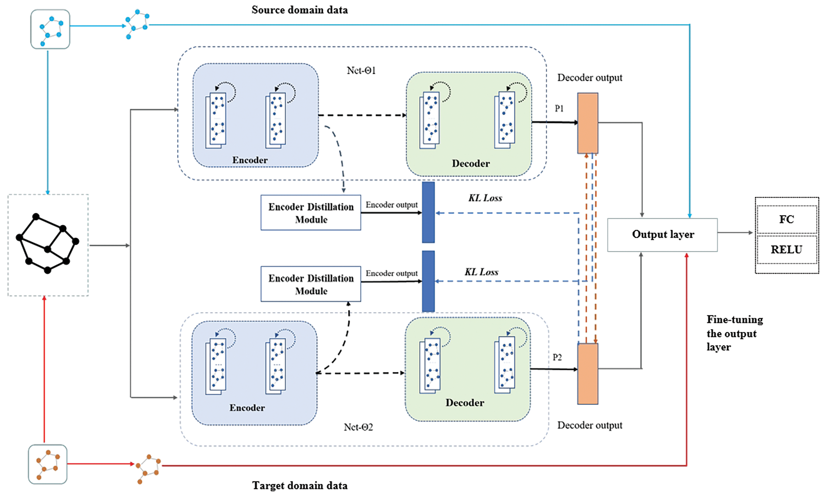
Figure 1: The TL-DKD model is a traffic flow prediction framework that combines transfer learning and deep knowledge distillation, comprising two encoder-decoder networks (Network 1 and Network 2). The encoder processes traffic data from the source domain to capture spatiotemporal patterns, with its layers frozen after training to retain these features. The decoder fine-tunes the encoded features for the target domain, minimizing information loss, while the output layer maps the refined features to final predictions and is fine-tuned for the target domain

3.1 Definition of the Prediction Problem

Traffic flow prediction is the process of modeling historical traffic data using mathematical models, machine learning, or deep learning techniques to estimate future or specific time period traffic conditions. This can be represented by the following mathematical model:

[X(m−M0+1),⋯,X(m);G]⟶f(⋅)[X(m+1),⋯,X(m+M)](1)

where X represents historical features such as traffic flow, speed, occupancy, and other related variables, G represents the traffic network modeled as a graph, and f(⋅) is the mapping function, which maps historical traffic data to a future time point. This function must be optimized through training.

3.2 Traffic Flow Prediction Model Using Transfer Learning

To validate the prediction performance of the complex model based on transfer learning, this paper utilizes a deep knowledge distillation (DKD) [28] model for transfer learning. The model, trained on the source domain, is transferred to the target domain task and fine-tuned with target domain data to enhance performance. The combination of transfer learning and deep knowledge distillation is referred to as TL-DKD. The DKD model introduces mutual learning and self-distillation algorithms based on the diffusion convolutional recurrent neural network (DCRNN) model [29]. Self-distillation, a model compression technique, improves performance through knowledge transfer within the model. Mutual learning, a special form of distillation, enhances efficiency and performance without requiring a pre-trained teacher model, as two student models learn from each other.

This paper uses DCRNN as the benchmark model, representing traffic flow as a diffusion process on a directed graph, capturing spatial features through random walks, and combining GRU gated units to extract temporal features. It employs a sequence-to-sequence framework and predetermined sampling to predict traffic flow. Fig. 2 shows the network architecture of DCRNN, which utilizes an encoder-decoder structure. The encoder converts an indefinite-length input sequence into a fixed-length context variable, while the decoder decodes this variable into an output sequence. By modeling the road network as a directed graph, nodes represent detectors, and the diffuse convolution layer is used to extract spatial correlations between nodes. GRU is utilized to capture temporal dependencies, and the diffuse convolution replaces the matrix operation in GRU to form a diffuse convolutional gated recurrent unit. The decoder structure is similar to that of the encoder and is used for the final traffic flow prediction.

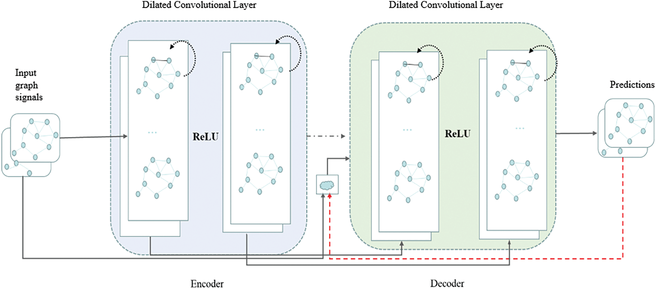
Figure 2: The DCRNN model architecture is depicted in the diagram. This model combines diffusion convolution for spatial dependency capture and GRU for temporal dependency modeling. The encoder-decoder structure processes traffic data, with the encoder converting input sequences into context variables and the decoder generating traffic flow predictions

To further enhance traffic flow prediction performance, a mutual learning and self-distillation algorithm was introduced on top of the graph neural network DCRNN, constructing the DKD model. As illustrated in Fig. 1, mutual learning is employed to build two networks with identical structures, enabling bidirectional distillation during the training process. This means that the two networks can learn from each other’s prediction results and update their own parameters and outputs based on these results. In the case of self-distillation, the network is divided into shallow and deep structures, with the deep structure acting as a teacher network to guide the shallow structure’s learning. This self-supervised approach helps the model better extract and utilize data features, thereby improving the model’s prediction performance.

During model training, two loss functions are used: the kullback-leibler (KL) divergence and cross-entropy loss (CE Loss). The KL divergence measures the similarity between the predicted probability distributions of the two networks, while the cross-entropy loss evaluates the alignment between predicted results and true labels. Overall, the total loss of the TL-DKD model consists of three components: cross-entropy loss, mutual learning loss, and self-distillation loss. Specifically, they are as follows:

Lθ1=(1−α)CELoss1+αDKL(P2∥P1)+KL(qEθ1,qDθ2)(2)

Lθ2=(1−α)CELoss2+αDKL(P1∥P2)+KL(qEθ2,qDθ1)(3)

where α is a weight coefficient used to measure the proportion of the mutual learning loss in the total loss, which is set to 0.5 in the experiments [28]. qEθ1 represents the encoder output of Net−Θ1, and qDθ2 represents the decoder output of Net−Θ2. Similarly, qEθ2 represents the encoder output of Network 2, and qDθ1 represents the decoder output of Network 1. KL(qEθ1,qDθ2) and represent the self-distillation loss and the mutual learning loss, respectively. P1 and P2 represent the predicted probabilities output by Networks 1 and 2 during training. CELoss1 and CELoss2 represent the cross-entropy losses of Net−Θ1 and Net−Θ2, respectively, while DKL(P2∥P1) and DKL(P1∥P2) represent the loss from mutual learning.

The TL-DKD model consists of three main components: an encoding layer, a decoding layer, and an output layer. The encoding layer serves as the feature extraction module, capturing the temporal and spatial dependencies of traffic data. It encodes traffic flow patterns into high-dimensional feature representations, which provide the foundation for subsequent predictions. During transfer learning, the encoding layer is frozen after training on the source domain to retain the general spatiotemporal features learned from the source data. This freezing strategy enhances the model’s generalization ability in the target domain, as traffic data from different regions often exhibit similar spatiotemporal patterns. By preserving these learned features, the model avoids the need to relearn them, saving both training time and computational resources.

Similarly, the decoding layer, which processes the high-dimensional features and transforms them into predictions for future traffic flow or speed, is also frozen after training on the source domain. This ensures that the prediction patterns learned from the source domain are retained and applied to the target domain, maintaining the model’s accuracy and robustness. Freezing both the encoding and decoding layers significantly improves the efficiency of transfer learning, especially in scenarios with limited target domain data or large domain differences. This approach minimizes the need for extensive retraining while preserving the model’s ability to generalize across different traffic scenarios.

The output layer maps the features from the decoding layer into final predictions, such as traffic flow or speed. It adjusts the number of neurons and dimensions based on the specific requirements of the target domain task to ensure prediction accuracy. The core of the output layer is the fully connected (FC) layer, which transforms the hidden states from the decoding layer into outputs with dimensions that match the target predictions. The activation function, typically rectified linear unit for traffic flow prediction, introduces non-linearity into the model. During fine-tuning with target domain data, the primary focus is on configuring the dimensions of the fully connected layer to align with task requirements, ensuring optimal performance. This structured approach enables the TL-DKD model to efficiently adapt to new environments while maintaining high prediction accuracy.

Based on the above TL-DKD model, this paper defines traffic flow prediction as the following process:

1.    Determine the source domain dataset.

2.    Determine the target domain dataset.

3.    Train the model on the source domain data to learn the feature representations of the source domain data.

4.    Fine-tune the model on the target domain dataset by freezing the encoder and decoder layers, while adjusting the output layer.

5.    After training and fine-tuning, use the model to make predictions on the target domain dataset.

4  Experiments

4.1 Datasets

The effectiveness of our method is validated through experiments on two commonly used datasets, collected every 5-min. These datasets are split into training, validation, and test subsets, with proportions of 60%, 20%, and 20%, respectively. The detailed information of these datasets is shown in Table 1.

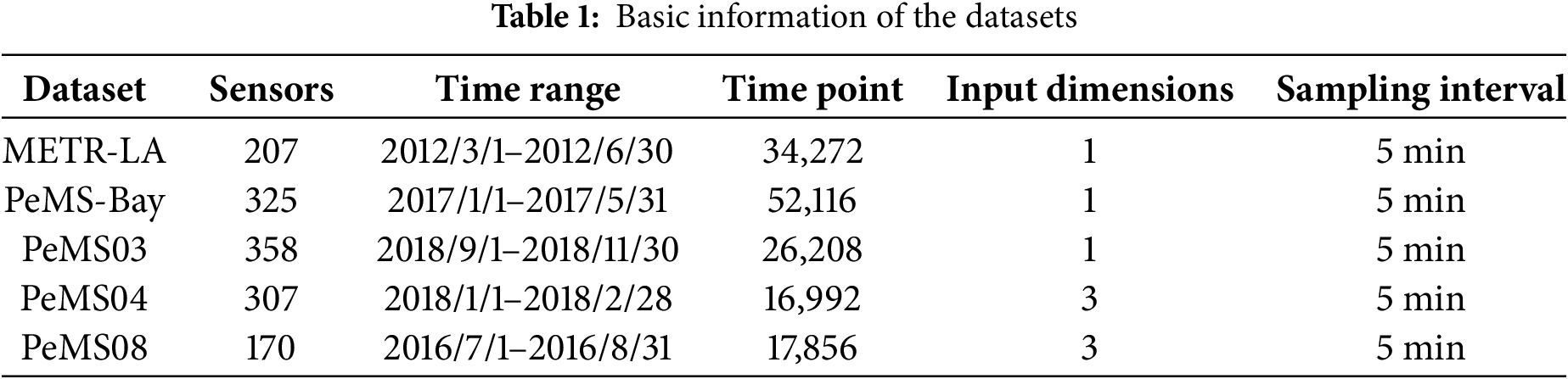
The METR-LA dataset covers 207 traffic detectors in the Los Angeles area, with data recorded from 1 March 2012 to 30 June 2012. The dataset records traffic speed features every 5 min, including key attributes such as traffic flow, speed, and occupancy. It contains a total of 34,272 data records.

The PeMS-Bay dataset is from the Bay Area of California, covering 325 traffic detectors, with data recorded from 1 January 2017 to 31 May 2017. The dataset records traffic flow and speed features every 5 min, totaling 52,116 data records.

The PeMS03 dataset covers 358 traffic detectors in the third district of California, with data recorded from 1 September 2018 to 30 November 2018 spanning 91 days. The dataset records traffic speed information every 5 min, totaling 26,208 data records.

The PeMS04 dataset covers 307 traffic detectors in the fourth district of California, with data recorded from 1 January 2018 to 28 February 2018 over 59 days. The dataset records traffic flow, occupancy, and speed features every 5 min, with a total of 16,992 data records.

The PeMS08 dataset covers 170 traffic detectors in the California region, with data recorded from 1 July 2016 to 31 August 2016 over 62 days. The dataset records traffic flow, occupancy, and speed features every 5 min, totaling 17,856 data records.

Table 1 presents a summary of two large-scale traffic flow datasets, each containing a substantial number of vehicle sensors. These sensors provide detailed traffic data and cover a broad spatial range, which makes them essential for traffic prediction. Fig. 3 illustrates the locations of the 207 sensors in the METR-LA dataset.

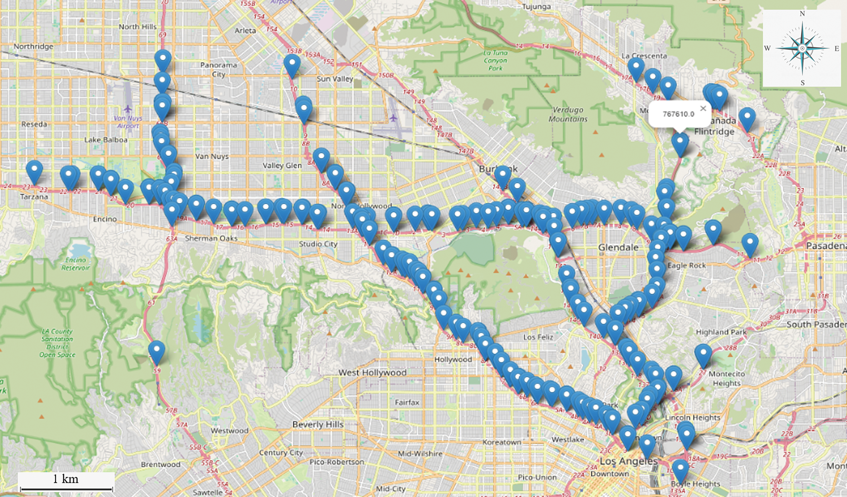
Figure 3: Visualization of sensors distribution in the METR-LA dataset

4.2 Experimental Settings

Baseline models: To validate the model’s effectiveness, this study employs multiple datasets and compares it against a series of baseline models, as described below:

1.    Vector Autoregressive (VAR) Model: A multivariate time series analysis model capable of capturing dynamic relationships between multiple sequences; however, the number of parameters increases with the number of variables.

2.    Support Vector Regression Model (SVR): A supervised learning model employed for classification and regression. It predicts by finding the optimal separating hyperplane or decision boundary, which requires proper parameter tuning.

3.    Long Short-Term Memory Network: A specialized recurrent neural network that addresses the gradient vanishing and explosion problems when processing long sequences, it requires adjustment of several hyperparameters.

4.    Diffusion Convolutional Recurrent Neural Network: A model that combines GCN and a variant of RNN, capturing spatial and temporal dependencies.

5.    Spatial-Temporal Graph Convolutional Network: A model that combines GCN and RNN to process spatial and temporal data separately, capturing dependencies and dynamic changes in the traffic network.

6.    Spatial-Temporal Synchronous Graph Convolutional Network: A model that introduces a synchronous mechanism to handle both temporal and spatial data simultaneously, effectively capturing local spatial-temporal correlations.

7.    Graph Wave Net: A model that combines graph convolution and dilated causal convolution to capture spatial-temporal correlations; it also learns an adaptive adjacency matrix through node embedding to handle hidden spatial dependencies.

8.    Multi-Range Attentive Bicomponent Graph Convolutional Network (MRA-BGCN) [30]: The MRA-BGCN model introduces a bicomponent graph convolution to model correlations between nodes and edges, as well as an attention mechanism to capture spatial features. Additionally, GRU is used to capture temporal features.

To evaluate the prediction performance of the optimized model, three metrics are used to assess the difference between true and predicted values: mean absolute error (MAE), mean absolute percentage error (MAPE), and root mean squared error (RMSE). The formulas for these metrics are as follows:

MAE=1n∑i=1n|yi−f(xi)|(4)

MAPE=100% n∑i=1n|yi−f(xi)yi|(5)

RMSE=1n∑i=1n(yi−f(xi))2(6)

where n represents the time steps for three metrics, yi and f(xi) denote the actual value and the predicted value at the i-th time step, respectively. The smaller the values of these three metrics, the higher the predictive accuracy of the model.

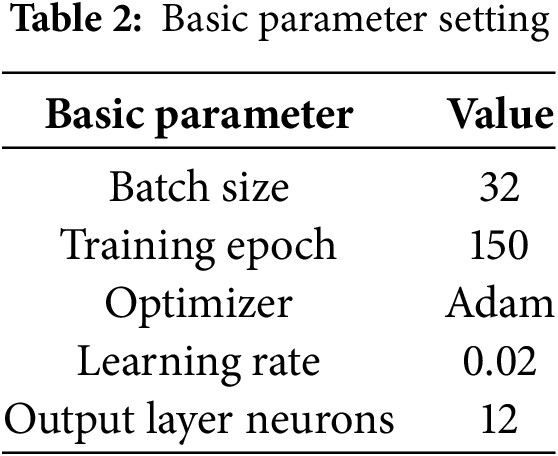
A grid search approach was used to optimize the performance of the TL-DKD model, identifying the optimal hyperparameters. A range of values was defined for key hyperparameters including learning rate, batch size, and number of neurons in the output layer. These hyperparameters were systematically evaluated using the training data to identify the best-performing combinations for traffic flow prediction. Basic parameter settings are shown in Table 2.

4.3 Experiment Results

4.3.1 Transfer Learning Based on Multi-Region Data

We have validated the model’s effectiveness under two distinct scenarios: one where traffic patterns and characteristics exhibit significant differences, and another where the data undergoes subtle changes. These experimental results demonstrate the model’s adaptability and performance across varying conditions. In the transfer learning based on multi-region data experiments, we initially used the METR-LA and PeMS-Bay datasets as source domain data for model training. Subsequently, the PeMS03, PeMS04, and PeMS08 datasets were used as target domain data for fine-tuning. To validate the model’s effectiveness in scenarios where traffic patterns and characteristics exhibit significant differences, as shown in Table 3, we evaluated the performance of the TL-DKD model on the PeMS03, PeMS04, and PeMS08 datasets. Due to the more diverse samples provided by the PeMS04 and PeMS08 datasets, the model was able to learn a broader range of feature representations, resulting in superior performance when dealing with unknown data.

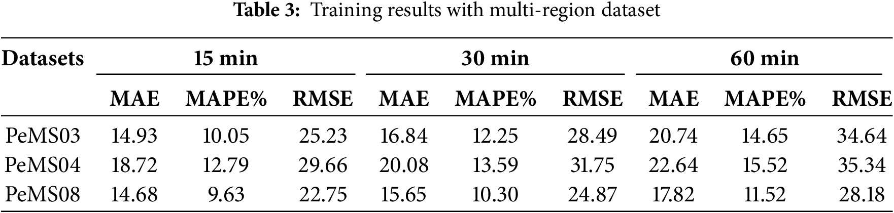
Table 4 provides a detailed performance comparison of various traffic flow prediction models on the PeMS03, PeMS04, and PeMS08 datasets for 30-min forecasts. The choice of a 30-min interval, it reduces computational burden, crucial for real-time applications like traffic signal control, while effectively capturing spatiotemporal traffic patterns. Table 4 includes a range of models, from traditional statistical models to advanced deep learning models, as well as the proposed models. The results clearly demonstrate the superior performance of the TL-DKD model across all datasets. For instance, on the PeMS04 dataset, TL-DKD achieves an MAE of 20.08, a MAPE of 13.59%, and an RMSE of 31.75, significantly outperforming models like VAR (MAE: 23.75, MAPE: 18.09%, RMSE: 36.66) and LSTM (MAE: 27.14, MAPE: 18.20%, RMSE: 41.59). Moreover, the table highlights the robustness of the TL-DKD model across different datasets. On the PeMS08 dataset, for example, TL-DKD achieves an MAE of 15.65, MAPE of 10.30%, and RMSE of 24.87, again significantly outperforming other models. The consistent performance across datasets underscores the model’s adaptability and generalization capabilities, making it an effective solution for traffic flow prediction, especially in data-scarce regions.

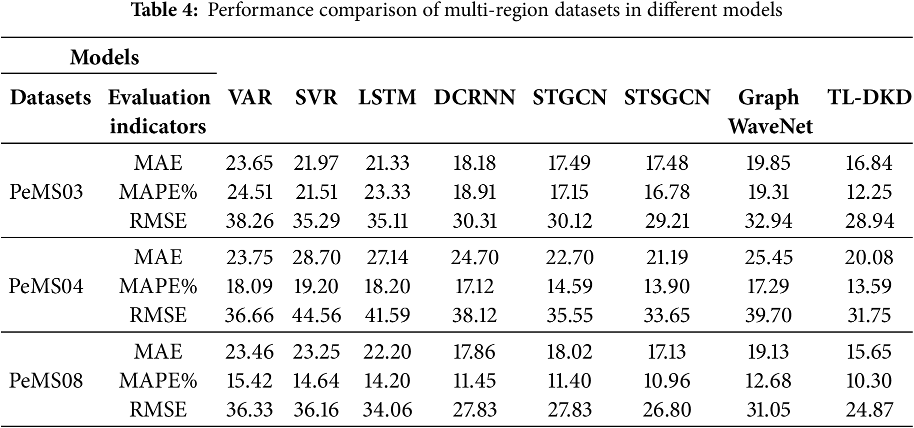
Fig. 4 provides a detailed comparison of the MAE for various models when applied to the PeMS03, PeMS04, and PeMS08 datasets. The results, presented with precision, indicate that the TL-DKD model performs exceptionally well across all datasets, significantly outperforming other benchmark models. This dominance is especially noticeable on the PeMS04 dataset, where the MAE of TL-DKD is 20.08, which is considerably lower than that of traditional models like VAR with a MAE of 23.75 and LSTM with a MAE of 27.14. This outcome suggests that the TL-DKD model exhibits greater adaptability and generalization capability in handling multi-region traffic data, especially in scenarios with data scarcity, thus significantly enhancing prediction accuracy. Other error metrics, such as MAPE and RMSE, also exhibit similar trends, further solidifying the superiority of the TL-DKD model.

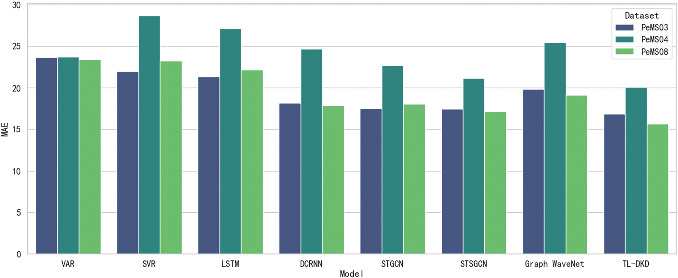
Figure 4: Model MAE comparison on PeMS datasets

We visualized the test loss of our model on the PeMS04 and PeMS08 datasets in Fig. 5. Fig. 5a shows the test loss variation on the PeMS04 dataset from 9 AM to 3 AM, while Fig. 5b illustrates the test loss over training steps on the PeMS08 dataset. A smoothing parameter of 0.6 was applied to reduce noise, with transparent lines represent raw data, while darker lines show smoothed curves. In Fig. 5a, the loss initially decreases rapidly and stabilizes around noon the next day, indicating quick early learning followed by slower convergence. Similarly, Fig. 5b shows a sharp initial drop in loss (around 5 k steps) and gradual flattening, reflecting rapid early learning and slower refinement toward optimal performance.

Figure 5: Test loss changes of TL-DKD on different datasets: (a) PeMS04; (b) PeMS08

4.3.2 Transfer Learning Based on Data Enhancement

To simulate subtle data variations in the transfer learning based on data enhancement experiments, we introduced random noise into the training data of the METR-LA and PeMS-Bay datasets. Noise augmentation serves as a form of regularization, helping to prevent overfitting, a common issue in deep learning where models learn not only relevant patterns but also noise and irrelevant variations, compromising their ability to generalize to new data. Initially, the model was pre-trained on the original, noise-free METR-LA and PeMS-Bay datasets to capture underlying patterns and ensure robust learning. Subsequently, noise was added to the PeMS-Bay data to simulate detector errors, serving as the source domain for training. This step enhanced the model’s adaptability to noisy data, enabling it to extract useful information despite the noise. The noise-augmented METR-LA dataset was then used as the target domain, further testing the model’s generalization capability in real-world scenarios where input data may differ from the training set.

Augmenting the training data with random noise introduces controlled variability into the learning process, helping the model become less sensitive to specific noise patterns and outliers in the training data. As a result, the model focuses more on underlying, consistent patterns in the traffic data, such as spatiotemporal dependencies and traffic flow trends, rather than memorizing irrelevant noise. This reduces the model’s sensitivity to noise and improves its generalization to new, unseen traffic data from different regions, time periods, or environmental conditions, each with varying levels of noise or disruptions.

Table 5 presents performance of multiple models on noise-augmented data, including VAR, SVR, LSTM, DCRNN, STGCN, Graph WaveNet, MRA-BGCN, DKD, and TL-DKD. Comparison of results reveals that the TL-DKD model consistently performs well, particularly in the long-term 60-min forecast, where TL-DKD achieves an MAE of 3.37, significantly outperforming other models. For example, DCRNN achieves an MAE of 3.60, and DKD an MAE of 3.53. This demonstrates that the TL-DKD model exhibits stronger robustness and prediction accuracy under noise-augmented data. In the short term, noise augmentation may increase error metrics, as the model must adapt to changes in the data caused by the added noise. However, over the long term, the model adapts to the noise and learns useful information, enhancing its robustness and improving its ability to generalize to unseen data.

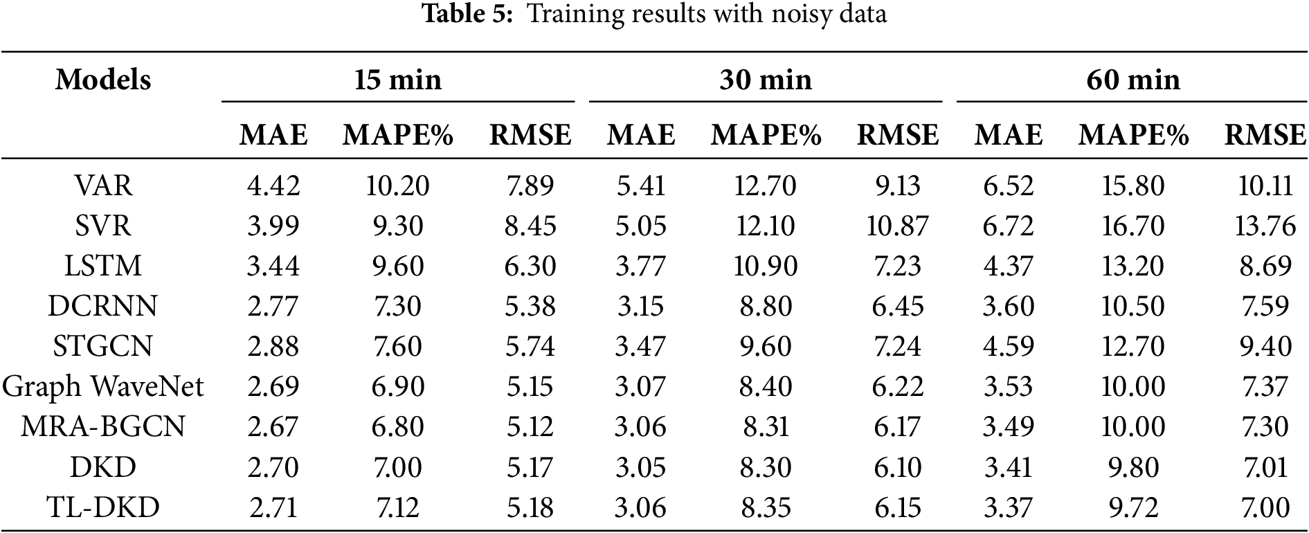
The MRA-BGCN model performs well in the 15 and 30-min forecasts, with MAEs of 2.67 and 3.06, respectively. However, in the 60-min forecast, its MAE rises to 3.49, slightly higher than TL-DKD’s MAE of 3.37. This suggests that MRA-BGCN excels in short-term predictions but is slightly less effective in long-term forecasts compared to TL-DKD. The DKD model, which enhances feature extraction capabilities through self-distillation and mutual learning mechanisms, shows stable performance across 15, 30, and 60-min predictions, with MAEs of 2.70, 3.05, and 3.41, respectively. Although DKD performs well, its MAE in the 60-min forecast is slightly higher than that of TL-DKD, indicating that TL-DKD further improves performance by incorporating transfer learning.

Fig. 6 shows the comparison between predicted values and actual values for the TL-DKD model under noisy enhanced data. From the figure, it can be observed that despite the introduction of random noise into the data, the predicted curve of the TL-DKD model still closely follows the trend of actual traffic flow variations. This indicates that the model can effectively capture the spatial and temporal dependencies of traffic flow and maintain a high level of prediction accuracy in the presence of noise disturbances.

Figure 6: Comparison of predicted values and actual values

Fig. 7 shows a comparison of MAE, MAPE, and RMSE for different models under noise-enhanced data across prediction intervals of 15, 30, and 60 min. The results indicate that the TL-DKD model performs best in long-term prediction at 60 min, with an MAE of 3.37, surpassing both DCRNN (3.60) and DKD (3.53). Although MRA-BGCN performs well in short-term predictions, TL-DKD demonstrates greater robustness and accuracy in long-term forecasts, suggesting higher adaptability and precision under noisy data conditions.

Figure 7: Comparative predictive results of TL-DKD with recent models: (a) MAE; (b) MAPE; (c) RMSE

5  Conclusion

This paper focuses on traffic flow prediction using data migration techniques. It begins by introducing the DCRNN model and then incorporates knowledge distillation to propose an advanced model called DKD. The paper thoroughly analyzes the prediction principles and performance of the DKD model, followed by the application of transfer learning techniques to optimize the DKD model, resulting in the TL-DKD model. Experimental results validate the effectiveness of the data migration strategy in scenarios with both significant differences in traffic patterns and subtle data variations. In both cases, the TL-DKD model leverages transfer learning to identify common features across tasks, ensuring robust performance in new environments. This enhances the model’s adaptability and robustness in real traffic scenarios, improving its generalization capabilities under varying data constraints.

A promising direction for future research lies in the deeper integration of traffic flow prediction models with adaptive traffic signal control systems. By enhancing the predictive capabilities of models to incorporate real-time data from signalized intersections, we can develop more dynamic and responsive traffic management solutions. Specifically, utilizing advanced machine learning techniques to predict traffic volumes and patterns at signalized intersections would enable preemptive adjustments in signal timings, optimizing traffic flow and reducing congestion. Ultimately, the synergy between traffic flow prediction and signal control holds significant potential to enhance urban traffic efficiency and sustainability.

Acknowledgement: None.

Funding Statement: This study was supported by the National Natural Science Foundation of China (Grant No. 52002031), and the Shaanxi Province Key R&D Plan Project (No. 2024GX-YBXM-002).

Author Contributions: Ying Li: Conceptualization, Determination of research questions, Selection of research methods. Haocheng Sun: Literature review, Data processing, Experimental operation, Writing—original draft. Ping Li: Experimental design, Data curation, Experimental operation. All authors reviewed the results and approved the final version of the manuscript.

Availability of Data and Materials: The datasets used and analyzed during the current study are available in the https://drive.google.com/drive/folders/1g5v2Gq1tkOq8XO0HDCZ9nOTtRpB6-gPe (accessed on 15 February 2025).

Ethics Approval: Not applicable.

Conflicts of Interest: The authors declare no conflicts of interest to report regarding the present study.

References

1. Pan B, Demiryurek U, Shahabi C. Utilizing real-world transportation data for accurate traffic prediction. In: 2012 IEEE 12th International Conference on Data Mining; 2012 Dec 10–13; Brussels, Belgium: IEEE; 2012. p. 595–604. doi:10.1109/ICDM.2012.52. [Google Scholar] [CrossRef]

2. Williams BM, Hoel LA. Modeling and forecasting vehicular traffic flow as a seasonal ARIMA process: theoretical basis and empirical results. J Transp Eng. 2003;129(6):664–72. doi:10.1061/(ASCE)0733-947X(2003)129:6(664). [Google Scholar] [CrossRef]

3. Hong WC, Dong Y, Zheng F, Lai CY. Forecasting urban traffic flow by SVR with continuous ACO. Appl Math Model. 2011;35(3):1282–91. doi:10.1016/j.apm.2010.09.005. [Google Scholar] [CrossRef]

4. Guo G, Wang H, Bell D, Bi Y, Greer K. KNN model-based approach in classification. In: Proceedings of the OTM Confederated International Conference, on the Move to Meaningful Internet Systems 2003: CoopIS, DOA, and ODBASE; 2003; Catania, Italy. p. 986–96. [Google Scholar]

5. Belgiu M, Drăguţ L. Random forest in remote sensing: a review of applications and future directions. ISPRS J Photogramm Remote Sens. 2016;114:24–31. doi:10.1016/j.isprsjprs.2016.01.011. [Google Scholar] [CrossRef]

6. Zhang W, Yu Y, Qi Y, Shu F, Wang Y. Short-term traffic flow prediction based on spatio-temporal analysis and CNN deep learning. Transp A Transp Sci. 2019;15(2):1688–711. doi:10.1080/23249935.2019.1637966. [Google Scholar] [CrossRef]

7. Ma X, Yu H, Wang Y, Wang Y. Large-scale transportation network congestion evolution prediction using deep learning theory. PLoS One. 2015;10(3):e0119044. doi:10.1371/journal.pone.0119044. [Google Scholar] [PubMed] [CrossRef]

8. Jiang W, Luo J. Graph neural network for traffic forecasting: a survey. Expert Syst Appl. 2022;207(7):117921. doi:10.1016/j.eswa.2022.117921. [Google Scholar] [CrossRef]

9. Zhao L, Song Y, Zhang C, Liu Y, Wang P, Lin T, et al. T-GCN: a temporal graph convolutional network for traffic prediction. IEEE Trans Intell Transp Syst. 2020;21(9):3848–58. doi:10.1109/TITS.2019.2935152. [Google Scholar] [CrossRef]

10. Zhao Z, Chen W, Wu X, Chen PCY, Liu J. LSTM network: a deep learning approach for short-term traffic forecast. IET Intell Transp Syst. 2017;11(2):68–75. doi:10.1049/iet-its.2016.0208. [Google Scholar] [CrossRef]

11. Fu R, Zhang Z, Li L. Using LSTM and GRU neural network methods for traffic flow prediction. In: 2016 31st Youth Academic Annual Conference of Chinese Association of Automation (YAC); 2016 Nov 11–13; Wuhan, China: IEEE; 2016. p. 324–8. doi:10.1109/YAC.2016.7804912. [Google Scholar] [CrossRef]

12. Dai G, Ma C, Xu X. Short-term traffic flow prediction method for urban road sections based on space-time analysis and GRU. IEEE Access. 2019;7:143025–35. doi:10.1109/ACCESS.2019.2941280. [Google Scholar] [CrossRef]

13. Scarselli F, Gori M, Tsoi AC, Hagenbuchner M, Monfardini G. The graph neural network model. IEEE Trans Neural Netw. 2009;20(1):61–80. doi:10.1109/TNN.2008.2005605. [Google Scholar] [PubMed] [CrossRef]

14. Wu Z, Huang M, Zhao A. Traffic prediction based on GCN-LSTM model. Paper presented at: IoTSC; 2021; Kunming, China. [Google Scholar]

15. Ye X, Fang S, Sun F, Zhang C, Xiang S. Meta graph transformer: a novel framework for spatial-temporal traffic prediction. Neurocomputing. 2022;491(6):544–63. doi:10.1016/j.neucom.2021.12.033. [Google Scholar] [CrossRef]

16. Yu B, Yin H, Zhu Z. Spatio-temporal graph convolutional networks: a deep learning framework for traffic forecasting. arXiv:1709.04875, 2017. [Google Scholar]

17. Song C, Lin Y, Guo S, Wan H. Spatial-temporal synchronous graph convolutional networks: a new framework for spatial-temporal network data forecasting. Proc AAAI Conf Artif Intell. 2020;34(1):914–21. doi:10.1609/aaai.v34i01.5438. [Google Scholar] [CrossRef]

18. Liu D, Wang J, Shang S, Han P. MSDR: multi-step dependency relation networks for spatial temporal forecasting. In: Proceedings of the 28th ACM SIGKDD Conference on Knowledge Discovery and Data Mining; 2022; Washington, DC, USA: ACM. p. 1042–50. doi:10.1145/3534678.3539397. [Google Scholar] [CrossRef]

19. Li M, Zhu Z. Spatial-temporal fusion graph neural networks for traffic flow forecasting. In: Proceedings of the 35th AAAI Conference on Artificial Intelligence; 2021; Palo Alto, CA, USA. p. 4189–96. [Google Scholar]

20. Harrou F, Zeroual A, Kadri F, Sun Y. Enhancing road traffic flow prediction with improved deep learning using wavelet transforms. Results Eng. 2024;23(1):102342. doi:10.1016/j.rineng.2024.102342. [Google Scholar] [CrossRef]

21. Zeroual A, Harrou F, Sun Y. Road traffic density estimation and congestion detection with a hybrid observer-based strategy. Sustain Cities Soc. 2019;46(2):101411. doi:10.1016/j.scs.2018.12.039. [Google Scholar] [CrossRef]

22. Krishnakumari P, Perotti A, Pinto V, Cats O, Lint HV. Understanding network traffic states using transfer learning. Paper presented at: 21st international conference on intelligent transportation systems; 2018 Nov 4–7; Maui, HI, USA. [Google Scholar]

23. Lin BY, Xu FF, Liao EQ, Zhu KQ. Transfer learning for traffic speed prediction: a preliminary study. Paper presented at: AAAI conference on artificial intelligence; 2018 Feb 2–7; New Orleans, LA, USA. [Google Scholar]

24. Li J, Guo F, Wang Y, Zhang L, Na X, Hu S. Short-term traffic prediction with deep neural networks and adaptive transfer learning. In: 2020 IEEE 23rd International Conference on Intelligent Transportation Systems (ITSC); 2020 Sep 20–23; Rhodes, Greece: IEEE; 2020. p. 1–6. doi:10.1109/itsc45102.2020.9294409. [Google Scholar] [CrossRef]

25. Yao Z, Xia S, Li Y, Wu G, Zuo L. Transfer learning with spatial-temporal graph convolutional network for traffic prediction. IEEE Trans Intell Transp Syst. 2023;24(8):8592–605. doi:10.1109/TITS.2023.3250424. [Google Scholar] [CrossRef]

26. Mallick T, Balaprakash P, Rask E, Macfarlane J. Transfer learning with graph neural networks for short-term highway traffic forecasting. Paper presented at: 25th International conference on pattern recognition (ICPR); 2021 Jan 10–15; Milan, Italy. [Google Scholar]

27. Zhang Z, Yang H, Yang X. A transfer learning-based LSTM for traffic flow prediction with missing data. J Transp Eng Part A Syst. 2023;149(10):04023095. doi:10.1061/JTEPBS.TEENG-7638. [Google Scholar] [CrossRef]

28. Li Y, Li P, Yan D, Liu Y, Liu Z. Deep knowledge distillation: a self-mutual learning framework for traffic prediction. Expert Syst Appl. 2024;252(3):124138. doi:10.1016/j.eswa.2024.124138. [Google Scholar] [CrossRef]

29. Li Y, Yu R, Shahabi C, Liu Y. Diffusion convolutional recurrent neural network: data-driven traffic forecasting. arXiv:1707.01926, 2017. [Google Scholar]

30. Chen W, Chen L, Xie Y, Cao W, Gao Y, Feng X. Multi-range attentive bicomponent graph convolutional network for traffic forecasting. Proc AAAI Conf Artif Intell. 2020;34(4):3529–36. doi:10.1609/aaai.v34i04.5758. [Google Scholar] [CrossRef]