Reinforcement Learning for Solving the Knapsack Problem

1  Introduction

Knapsack problem is a classical combinatorial optimization problem which has been widely used in applied mathematics and computer science for decades. For example, in cloud computing, a server can host multiple virtual machines. Consider server resource allocation: administrators must select virtual machines that maximize computational performance while respecting finite memory constraints—a direct manifestation of knapsack optimization principles. Knapsack problem is classified as an NP-hard problem and many exact and heuristic algorithms have been proposed [1–4]. In its simplest form, the problem involves a set of items, each with a specific weight, volume, and value, and the goal is to determine the optimal selection of items that maximizes the total value without exceeding a given capacity constraint. Over the years, the knapsack problem has been extensively studied, and a variety of solution approaches have been proposed, ranging from exact algorithms such as dynamic programming (DP) to heuristic methods and approximation algorithms. Dynamic programming (DP) achieves theoretical optimality but becomes computationally prohibitive due to exponential time complexity growth with problem scale. While mathematically rigorous, DP implementations struggle with real-world scalability. In contrast, heuristic methods, such as greedy algorithms, genetic algorithms, and simulated annealing, are often employed for larger problem instances due to their faster execution times. However, these heuristic methods come with significant limitations. Traditional methods cannot iteratively refine solutions through environmental feedback, rendering them ineffective for dynamic scenarios. Genetic algorithms and simulated annealing demonstrate particular vulnerability when handling evolving constraints or variable capacity conditions. Consequently, while heuristics can provide quick solutions, they are often less reliable in achieving high-quality solutions, particularly when the problem space is large and complex.

Reinforcement learning (RL) is a subfield of machine learning. Using deep neural networks [5] as function estimators within an RL system [6,7], deep reinforcement learning (DRL) has been shown to be effective in many areas including Atari games [8], Go game [9], dialog systems, text generation, computer vision, and robotics. DRL can be considered as a step towards embodying universal artificial intelligence [10]. It has recently emerged as a promising approach to tackle combinatorial optimization problems like the knapsack problem. The knapsack problem involves selecting a subset of items to maximize total value while adhering to weight and volume constraints. RL is particularly well-suited for this type of problem because it excels in environments where an agent must make a series of sequential decisions. In the knapsack problem, for each item, the agent must decide whether to include it in the knapsack or not, subject to the available capacity constraints. RL allows the agent to learn a policy that maps states (current capacity and item selection) to actions (deciding which item to select), with the goal of maximizing cumulative rewards (i.e., total value). As the agent interacts with the environment, it learns from experience and adjusts its policy to improve future decisions. This decision-making process aligns well with the knapsack problem, where the optimal solution depends on a sequence of choices that balance the trade-offs between item values and the available capacity. Through iterative learning, RL can find near-optimal solutions more efficiently than traditional methods, especially for large-scale problems with many items. A flowchart in Fig. 1 is included to provide a clear, intuitive view of RL-based approach for knapsack problem and its components. While RL has been successfully applied to various optimization problems, its application to the knapsack problem remains an area of active research. Traditional RL methods face challenges related to the state representation, exploration of the solution space, and efficiency of training, especially when dealing with problems with large action and state spaces.

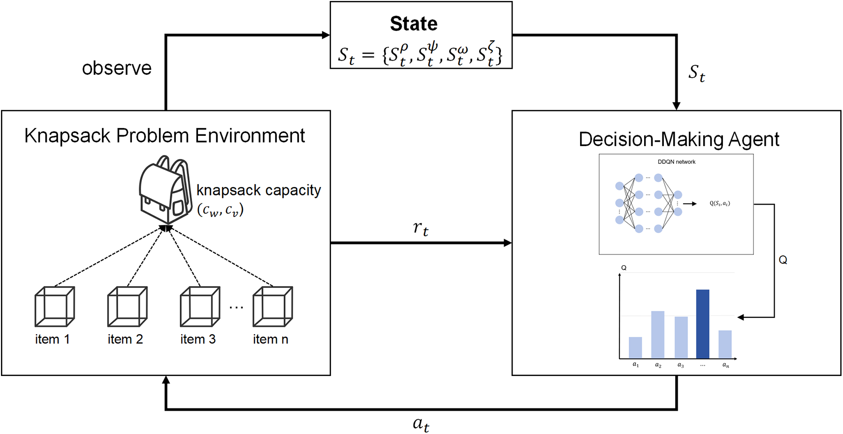
Figure 1: An overall framework for a reinforcement learning-based system for solving the knapsack problem. We formally define a backpack problem environment (left part) and develop a reinforcement learning-based decision-making agent (right part) to interact with the environment and automatically learn solution strategies under capacity and volume constraints

In this paper, we propose a novel approach to solve the knapsack problem using RL by enhancing both the state representation and the neural network architecture. First, we introduce a key modification to the state representation: instead of using raw item weights, volumes, and values, we transform them into ratios relative to the knapsack capacity. Specifically, we express the weights and volumes of items as proportions of the knapsack’s total capacity, and item values are represented as their percentage contribution to the total value of all items. These normalized representations streamline learning across varying problem scales, eliminating unit dependency and enhancing generalization. Benchmarked against leading RL methods like Transformer-based approaches, our state-space modification delivers 5% accuracy gains. Computational efficiency improvements prove more dramatic: the RL framework operates 9000× faster than DP implementations while handling capacity-constrained scenarios. Building on this improvement, we further enhance the RL model’s performance by introducing Noisy layers into the neural network architecture. By injecting parametric stochasticity, these layers prevent premature convergence to suboptimal solutions through enhanced exploration. Combined with the revised state representation, this modification yields incremental accuracy improvements of 0.2%–0.5%. This further boost highlights the importance of incorporating exploration mechanisms into RL models for solving combinatorial optimization problems.

The contributions of this paper are as follows:

1. State Modification: We propose a novel state representation for the knapsack problem, where item weights and volumes are expressed as ratios relative to the knapsack capacity, and item values are represented as percentages of the total value. This leads to a significant improvement in model performance.

2. Neural Network Enhancement with Noisy Layers: We introduce Noisy layers into the neural network architecture used by the RL agent, further improving the model’s accuracy and exploration efficiency.

3. Efficiency and Accuracy Comparison: We demonstrate that our RL approach, with the proposed state modifications and Noisy layers, outperforms traditional dynamic programming (DP) in terms of execution time (with a 9000× speedup). Additionally, our method surpasses the best existing RL algorithms, such as the Transformer model [11], by a significant margin.

The rest of the paper is organized as follows: Section 2 reviews related work on solving the knapsack problem and applying RL to combinatorial optimization. Section 3 details the methodology, including the problem formulation, state representation, neural network architecture, and training procedure. In Section 4, we present experimental results, comparing our approach with existing methods in terms of accuracy and execution time. Finally, Section 5 discusses the implications of our results, identifies potential limitations, and outlines directions for future work.

2  Related Work

2.1 Overview of Knapsack Problem Solving Methods

The knapsack problem (KP) is a classical combinatorial optimization problem that has been extensively studied, with various methods proposed to solve it efficiently. Martello and Toth evaluated both exact and approximate algorithms for solving KP [12], including branch-and-bound algorithms, dynamic programming (DP), and hybrid approaches that combine both. These algorithms were benchmarked against randomly generated sample items, with approximate algorithms mainly based on greedy approaches or scaling methods. While these methods provide solutions in a reasonable time frame, they often fall short in large or complex problem instances. In particular, DP’s exponential time complexity becomes a significant bottleneck as the number of items increases, and greedy algorithms may fail to find optimal solutions, especially when problem parameters are nonlinear or non-convex. This presents a need for more adaptive and scalable approaches, such as reinforcement learning (RL), which can continuously refine its strategy through interaction with the environment. In cases where item weights are not known a priori, Kosuch and Lisser proposed solutions for solving the knapsack problem with uncertain item weights, either through single-stage or two-stage decision-making processes. The two-stage decision method, which allows for adjustments after initial decisions, was shown to be more accurate [13]. However, these methods are still limited by the assumption that all decisions are made based on available knowledge at the time, which does not account for the dynamic nature of real-world decision-making, where uncertainty can evolve over time. Our RL-based approach addresses this challenge by enabling the agent to learn and adapt its decisions over time through feedback, improving its ability to handle uncertainties and unknowns in real-time. Chu and Beasley used genetic algorithms to propose a heuristic for solving multidimensional KP, demonstrating that high-quality solutions could be found within a reasonable computational time [14]. While genetic algorithms offer flexibility and have been successful in finding approximate solutions, they typically require multiple iterations to converge to a satisfactory solution, and the results can vary depending on the parameter settings. By contrast, our approach, which leverages RL, continuously improves its decision-making through trial and error, offering more reliable convergence to optimal or near-optimal solutions, particularly in large-scale problems where traditional methods may struggle. Sahni presented approximate solutions for KP that require polynomial time complexity and linear storage, providing near-optimal results for most problem instances [15]. However, these methods often lack of the adaptability to respond to dynamic changes in the problem space, limiting their effectiveness in real-time or evolving environments. RL, on the other hand, excels in such settings, as it is capable of continuously learning from the environment and adjusting its strategy based on new information. Kulkarni and Shabir introduced cohort intelligence algorithms inspired by social learning to solve KP, showing that their method yielded satisfactory results at reasonable computational costs [1]. However, while cohort intelligence methods are effective in certain problem instances, they still rely on predefined rules and may not fully explore the solution space as efficiently as RL-based approaches. Our method, incorporating Noisy layers into the neural network architecture, addresses this limitation by improving the exploration of the state-action space, resulting in more effective optimization in complex environments.

2.2 Reinforcement Learning Approaches for Combinatorial Optimization

Reinforcement learning (RL) has gained traction in solving combinatorial optimization problems, including the knapsack problem. Early works in this area focused on adapting RL to other combinatorial problems such as the traveling salesman problem and vehicle routing. Bello et al. introduced two RL-based approaches for combinatorial optimization, including pretraining using recurrent neural networks and active search, which was tested on the traveling salesman problem but was suggested to be applicable to KP as well [16].

Further innovations in RL include the integration of attention mechanisms to improve the efficiency of the learning process. For example, Nazari et al. incorporated attention mechanisms in a recurrent neural network (RNN) model for vehicle routing, emphasizing the ability of attention to handle both static and dynamic elements in optimization tasks [17]. Similarly, Dai et al. used deep Q-learning with graphical embeddings for optimization problems like maximum cutting and traveling salesman [18]. Parisotto et al. proposed an RL architecture similar to transformers but with key differences in layer normalization and gating mechanisms to improve RL training consistency [19].

The application of RL specifically to the knapsack problem has seen some significant advancements. Gu et al. applied recurrent neural networks for KP, introducing a purely data-driven approach where the coefficients of each variable and the constraints were inputs for the model [20]. Denysiuk et al. leveraged binary classification using artificial neural networks for KP, where the parameters were adjusted using neuroevolution algorithms due to the unknown nature of target values [21].

Yildiz explored the use of deep Q-learning with various neural network models, including fully connected layers, attention mechanisms, and transformer encoder blocks to solve the knapsack problem [11]. This work demonstrated the effectiveness of transformer models in handling combinatorial optimization tasks like KP, offering improved performance compared to traditional methods and highlighting the potential of deep RL in this domain. The paper showed that attention-based models can capture the dependencies between different items in the knapsack, significantly improving the efficiency and accuracy of the solution process.

2.3 The Role of Neural Networks and Noisy Layers in Optimization Problems

Recent advancements in neural networks have introduced innovative techniques to improve the exploration and learning capacity of RL models. One such technique is the use of Noisy layers in neural networks. These layers add randomness to the weights, enhancing the exploration capabilities of the agent and preventing it from becoming stuck in suboptimal solutions during training [22]. This approach has shown promise in various RL applications, particularly in environments with large state and action spaces, such as combinatorial optimization problems.

In the context of the knapsack problem, adding Noisy layers to the neural network architecture has been shown to lead to incremental improvements in performance. In our work, we extend this idea by applying Noisy layers after modifying the state representation, which was already improved to a ratio-based format relative to the knapsack capacity. This combination of state modification and Noisy layers results in further accuracy gains, demonstrating the significant potential of this technique for combinatorial optimization problems like the knapsack problem.

3  Methodology

In this section, we describe the methodology used to solve the knapsack problem (KP) using Dueling DQN and incorporate a Markov Decision Process (MDP) formulation. We detail the state space representation, the action and reward definitions, and the training procedure, including the use of Noisy layers to enhance exploration.

3.1 Problem Formulation and Objective

The knapsack problem (KP) is a combinatorial optimization problem in which the goal is to select a subset of items to maximize total value, subject to constraints on both weight and volume. We assume that there is a total of n items. Each item i has: wi: weight of item i, vi: volume of item i, pi: value of item i, xi∈{0,1}: binary variable indicating whether item i is selected.

The knapsack has two capacity constraints: weight capacity (cw), and volume capacity (cv).

The objective is to maximize the total value of the selected items while adhering to the following constraints:

∑i=1nwixi≤cw,∑i=1nvixi≤cv

where cw and cv represent the maximum allowable weight and volume capacities of the knapsack, respectively. The total value of the selected items is calculated as:

Ptotal=∑i=1npixi

where pi is the value of item i and xi indicates whether the item is included in the knapsack. The goal is to maximize Ptotal, the total value, by choosing the most valuable items while respecting the weight and volume constraints.

3.2 Markov Decision Process (MDP) for Knapsack Problem

We model the knapsack problem as a Markov Decision Process (MDP), which is a sequential decision-making framework. In this formulation, the agent interacts with the environment to select a subset of items that maximizes the total value, while ensuring that the total weight and volume of the selected items do not exceed the knapsack’s capacity constraints.

At each decision step, the agent observes the current state, which includes information about the remaining capacity of the knapsack and the items considered for inclusion. Based on this state, the agent chooses an action, which corresponds to selecting an item to add to the knapsack. The action results in a transition to a new state, where the knapsack’s remaining capacity is updated based on the weight and volume of the selected item. The agent receives a reward equal to the value of the selected item.

The objective of the agent is to maximize the cumulative reward, which corresponds to maximizing the total value of the selected items while adhering to the weight and volume constraints. This process of decision-making and feedback continues until all items are evaluated, and the agent learns an optimal policy to solve the knapsack problem.

•      State Space (S): The state is represented by a vector St={tρS,tψS,tωS,tζS}∈R4×(n+1), where each row corresponds to an item and contains four values:

1.    Selection Status (tρS): A binary value xi∈{0,1} indicating whether item i has been selected (1) or not (0).

2.    Value Coefficient (tψS): The normalized value of item i calculated as piPtotal′, where pi is the value of item i and Ptotal′ is the total value of all items. This helps the agent understand the relative importance of items.

3.    Weight Coefficient (tωS): The normalized weight of item i, calculated as wicw, where wi is the weight of item i and cw is the weight capacity of the knapsack. This coefficient ensures that the weight of each item is considered relative to the total knapsack capacity.

4.    Volume Coefficient (tζS): The normalized volume of item i, calculated as vicv, where vi is the volume of item i and cv is the volume capacity of the knapsack.

The last row of the matrix represents the knapsack’s remaining capacity, with initial values set to 1, indicating full capacity. The coefficients for weight, volume, and value are all normalized as previously described.

•      Action Space (A): The action at each step corresponds to the selection of an item to place in the knapsack. The agent chooses an item based on its current state representation. The action space is defined as the set of all items ai∈{1,2,…,n}, where n is the number of items. The agent’s goal is to make a decision such that the total weight and volume do not exceed the knapsack’s capacity while maximizing the total value.

•      Transition Function (T): The transition function defines the state transition probabilities based on the current state st and selected action at. In this problem, the transition is deterministic, meaning that when an action is taken (i.e., an item is selected), the new state st+1 is fully determined by the action and the current state: st+1=T(st,at).

This transition updates the selection status of the item chosen (xi=1) and decreases the remaining weight and volume capacities of the knapsack by the corresponding values of the selected item. The remaining capacity is updated as:

remaining weight =cw−∑i−1nwi⋅xi(1)

remaining volume =cv−∑i−1nvi⋅xi(2)

•      Reward Function (R): The reward function provides feedback to the agent based on the action taken. The reward is defined as the value of the item selected for addition to the knapsack. If the item can be added without violating the weight or volume constraints, the agent receives a reward equal to the value of the item pi. If the item cannot be added (i.e., the knapsack’s capacity would be exceeded), the reward is 0.

rt={piif item i is added to the knapsack,0 if item i cannot be added due to capacity constraints.(3)

The reward function is designed to encourage the agent to select high-value items while adhering to the knapsack’s capacity constraints. The overall goal is to maximize the sum of the rewards, i.e., the total value of the selected items.

3.3 Enhancements in State Representation and Modifications

As previously mentioned, the state consists of the normalized weight, volume, and value coefficients for each item. This state formulation allows the agent to learn effectively, without being influenced by the absolute values of the items.

•      Normalized Weight and Volume: Each item’s weight wi and volume vi are normalized by the knapsack’s corresponding capacities cw and cv. This ensures that the state representation is independent of the absolute values of weight and volume and allows for more consistent decision-making across different instances of the problem: wi′=wicw,vi′=vicv. This normalization ensures that the agent operates on scaled, dimensionless features, making the state space more manageable.

•      Normalized Value: The value of each item is expressed as a percentage of the total value across all items. This helps the agent focus on relative item values instead of absolute values, making learning more efficient: pi′=piPtotal′, where Ptotal′ is the sum of the values of all items in the current problem instance.

The modified state space thus consists of the normalized weights, volumes, and values of all items, which is a more compact and consistent representation of the problem.

3.4 Dueling DQN for Solving Knapsack Problem

Dueling DQN (DDQN) [23] is an enhancement over the DQN [8], which decomposes the Q-value into two distinct streams: one for the state-value function which estimates V(s)∈R and another for estimating the advantage function A(s,a)∈R.

•      State Value Function V (s): Represents the expected value of being in state s, independent of the action selected.

•      Advantage Function A (s, a): Measures how much better action □ is compared to other actions in state s.

The Q-value function is estimated as:

Q(s,a)=V(s)+A(s,a)−1|A|∑a′A(s,a′)(4)

This decomposition allows for more stable learning, as the agent can independently estimate the value of a state and the advantage of each action.

The Q-value update follows the Bellman equation:

Q(st,at)←Q(st,at)+α(rt+γmaxa′Q(st+1,a′)−Q(st,at))(5)

where:

•      st and at are the current state and action,

•      rt is the immediate reward,

•      γ is the discount factor,

•      α is the learning rate.

To train the DDQN model, the Q-value estimation could be approximated towards some target Q-value computed from temporal difference learning [6], denoted as:

ytarget=r+γmaxa′Q(s′,a′;θ−)(6)

where θ−={h−θ,vhθ,vadvθ,} is the parameter for the target Qnetwork that is updated less frequently than DDQN network to prevent divergence during training, and r is the one-step reward computed following Eq. (3). To optimize the output of DDQN towards the ytarget, we employ the following loss:

LDDQN(θ)=E(s,a,r,a′)∼D[(ytarget−Q(s,a;θ))2](7)

where experience tuples (s,a,r,s′) are sampled from a reply buffer D to construct the mini-batch samples to update the network. The model parameters for DDQN are optimized by standard gradient-descent by backpropagating the following gradient w.r.t θ:

∇θLDDQN(θ)=E(s,a,r,a′)∼D[(ytarget−Q(s,a;θ)∇θQ(s,a;θ))](8)

3.5 Incorporating Noisy Layers for Improved Exploration

In reinforcement learning (RL), exploration vs. exploitation is a fundamental challenge. While traditional methods such as ∈-greedy exploration help the agent explore the environment, they often lead to inefficient exploration strategies. In environments where the problem space is large or highly dimensional, improper exploration can significantly hinder the learning process, leading to poor generalization and convergence issues. To address this, we incorporate Noisy layers into the neural network architecture, specifically in the DDQN framework, to improve exploration and subsequently enhance the overall performance of the agent in solving the knapsack problem.

3.5.1 Motivation for Using Noisy Layers

Noisy layers are a technique introduced to encourage intrinsic exploration by directly modifying the network’s parameters (weights and biases) during training. Rather than relying on fixed exploration strategies such as ∈ -greedy, noisy layers introduce stochasticity into the network itself, making the actions taken by the agent inherently more diverse. This stochasticity allows the agent to explore the environment in a more dynamic way, leading to better coverage of the state-action space, especially in complex, high-dimensional problems like the knapsack problem.

In traditional DQN models, the exploration-exploitation trade-off is addressed using a decaying ∈-greedy strategy. However, this approach may not be optimal, as it treats exploration as a fixed component that does not adapt to the learning progress of the agent. In contrast, Noisy layers provide a more sophisticated mechanism for exploration by introducing random noise directly into the neural network weights, which increases the model’s capacity to explore different parts of the state-action space.

3.5.2 Noisy Layers in DDQN

In the DDQN framework, the Q-values are decomposed into two separate components: the state-value function V (s) and the advantage function A (s, a). The Q-value function Q (s, a) is then calculated as the sum of these two components:

Q(s,a)=V(s)+A(s,a)−1|A|∑a′A(s,a′)(9)

The benefit of this decomposition is that it allows the model to better handle situations where some actions have no effect on the state, and thus their advantage should be near-zero. However, while this decomposition improves the stability and performance of the DQN model, it still suffers from the same exploration challenges inherent to traditional RL approaches.

By introducing Noisy layers into the network, we can make both the state-value function and the advantage function stochastic, which leads to more varied and potentially more optimal exploration during training. Specifically, the weights of the fully connected layers in both V (s) and A (s, a) are replaced with noisy versions of themselves. In practice, the noisy version of a weight w is typically generated using the following equation:

w′=w+σ⋅∈(10)

where w is the original weight, ∈ is a learnable parameter that controls the scale of the noise, ∈ is a random variable drawn from a noise distribution, typically Gaussian, i.e., ∈∼N(0,1).

Thus, each weight in the model becomes a distribution over possible values rather than a fixed value. During training, the noisy weights are updated, which allows the model to explore more diverse strategies for selecting actions based on the noisy estimations of Q-values. This introduces variability in the Q-value predictions and ultimately leads to a more robust learning process.

3.5.3 Benefits of Noisy Layers in the Knapsack Problem

For the knapsack problem, where the objective is to select the most valuable combination of items without exceeding the knapsack’s capacity constraints, Noisy layers offer several key advantages:

1.    Improved Exploration: The primary benefit of Noisy layers is their ability to improve exploration. By introducing randomness into the weights, the agent can explore a broader range of item combinations and packing strategies, which is crucial in combinatorial problems like the knapsack problem. This prevents the agent from getting stuck in suboptimal solutions, which is a common issue when relying solely on greedy or deterministic exploration strategies.

2.    Adaptive Exploration: Unlike fixed exploration strategies, Noisy layers adapt to the learning process. Initially, the noise may guide the agent to explore more areas of the state-action space, while later in training, as the noise is adjusted and reduced, the agent starts to exploit the most valuable solutions it has discovered. This gradual transition from exploration to exploitation allows the agent to converge faster and more reliably to an optimal or near-optimal solution.

3.    Handling High Dimensionality: The knapsack problem with large numbers of items (i.e., high-dimensional state and action spaces) presents a challenge for conventional RL methods. Noisy layers help to mitigate this challenge by enhancing the network’s ability to generalize across a vast state-action space, thus improving its ability to make efficient decisions even when the number of items in the knapsack grows.

4.    Faster Convergence: Since Noisy layers enable better exploration of the state-action space, the agent is able to discover the optimal or near-optimal combinations of items more quickly. This leads to faster convergence during training, which is particularly advantageous when solving large-scale knapsack problems.

3.5.4 Noisy Layers in Practice

In our implementation, Noisy layers are incorporated into both the value and advantage functions within the DDQN architecture. This modification helps improve the robustness of the Q-value estimates by introducing variability, which in turn enhances the exploration process. We add noise to the fully connected layers in both the V (s) and A (s, a) streams of the DDQN, allowing the agent to explore potential item combinations more effectively.

The noise parameters (σ) are learned during the training process, allowing the agent to adjust the level of noise based on its current state of knowledge. As the agent trains, the variance introduced by the Noisy layer’s decreases, allowing the model to transition toward more deterministic action selection, which is essential for efficient exploitation once the agent has sufficiently explored the problem space.

3.6 Training Procedure and Algorithm Optimization

The training procedure follows standard DQN with modifications for the MDP and dueling architecture:

1.    Initialization: The neural network weights are initialized randomly, and the agent starts by selecting actions randomly to explore the state space.

2.    Experience Replay: The agent stores state-action-reward transitions in an experience replay buffer, allowing the network to learn from past experiences and break temporal correlations between consecutive updates.

3.    Target Network: A target Q-network is periodically updated with the weights of the main Q-network to stabilize training.

4.    Q-Value Update: The Q-values are updated using the Bellman equation and gradient descent.

5.    Exploration-Exploitation Balance: The agent initially explores the state space with a high exploration rate and gradually shifts to exploitation.

6.    Early Stopping: Training stops when the agent achieves a predefined performance threshold or no significant improvement is observed.

3.7 Evaluation Metrics and Performance Criteria

The performance of the agent is evaluated based on the following metrics:

1.    Accuracy: The accuracy is computed as the ratio of the total value obtained by the agent to the optimal value, expressed as a percentage:

Accuracy=VagentVoptimal(11)

2.    Execution Time: The execution time of the DDQN approach is compared with traditional methods like DP to highlight the efficiency gains.

By using DDQN in combination with Noisy layers and a structured MDP representation, our approach efficiently solves large-scale knapsack problems, demonstrating improvements in both accuracy and execution time.

4  Experimental Setup and Results

To evaluate the performance of the proposed DDQN model without and with Noisy layers for solving the knapsack problem, we conducted experiments on two variants of the knapsack problem:

•      Standard two-dimensional knapsack problem: Each item can be selected at most once (xi∈{0,1}). The result for the problem will be shown in Table 1.

•      Extended two-dimensional bounded knapsack problem: Items can be selected multiple times with upper bounds (xi∈{0,1,…,bi}) under dynamic item quantities. The result for the problem will be shown in Table 2. For example, the problem can be used in logistics optimization: Loading cargo batches with weight and volume limits (e.g., shipping containers), and the same type of cargo can be loaded for multiple times. In addition, the problem can be used in Inventory Management: Restocking products with limited warehouse space and budget, and the same type of product can be restocked for multiple times. Moreover, the problem can be used in Cloud Resource Allocation: Assigning variable virtual machine (VM) instances to servers with CPU/memory constraints, and the same type of VM instances can be assigned for multiple times.

We compared the performance of the DDQN model without and with Noisy layers (i.e., DDQN, Dueling DQN with Noisy layers) against traditional algorithms (e.g., DP, Greedy, Random) on both problem variants.

4.1 Experimental Design and Setup Details

The knapsack is constrained by weight and volume capacities, where the capacity values depend on the problem variant:

•      For the Two-Dimensional Bounded Knapsack Problem (2D-BKP), capacities are defined as weight capacity cw=n×80 and volume capacity cv=n×80, where n is the number of items.

•      For the baseline 0–1 knapsack problem, capacities are set to cw=cv=n×30.

Each item i has a weight wi, volume vi, and value pi, all randomly generated from the uniform distribution U(1,100). In the extended 2D-BKP variant, each item additionally has a maximum allowable quantity bi∼U(1,5), making the selection variable xi∈{0,1,…,bi}, whereas in the 0–1 knapsack xi∈{0,1}.

To evaluate the performance of our algorithms, we conduct experiment on five different algorithms (i.e., DP, Greedy Algorithm, Random Selection, DDQN, Dueling DQN with Noisy layers) using two sets of item sizes (n∈{10,20,30} and n∈{5,10,15}) for two different problems. Specifically, DP, Greedy Algorithm, Random Selection are the baseline algorithms, and DDQN, Dueling DQN with Noisy layers are our proposed algorithms. All results were averaged over 1000 randomized samples to ensure statistical reliability.

DP was used as a baseline to provide the optimal solution. DP for the 2D-BKP problem solutions were only computed for n≤15, since itstime complexity is O(n⋅cw⋅cv), which is very high for large n.

•      Greedy Algorithm selects items based on the highest value-to-weight ratio, providing a fast but potentially suboptimal solution.

•      Random Selection is a baseline that selects items randomly, allowing us to evaluate how far non-optimized solutions deviate from optimal ones.

•      DDQN and Dueling DQN with Noisy layers (DDQN-Noisy) were the reinforcement learning-based models tested, with the former serving as a baseline for RL and the latter being an improvement aimed at enhancing exploration. It is noteworthy that the state space is represented as a matrix of dimensions (n+1)×4, where the first n rows encode item features (xi,pi,wi,vi) and the last row tracks the knapsack’s remaining capacities.

4.2 Experimental Results and Comparison

4.2.1 Accuracy Comparison

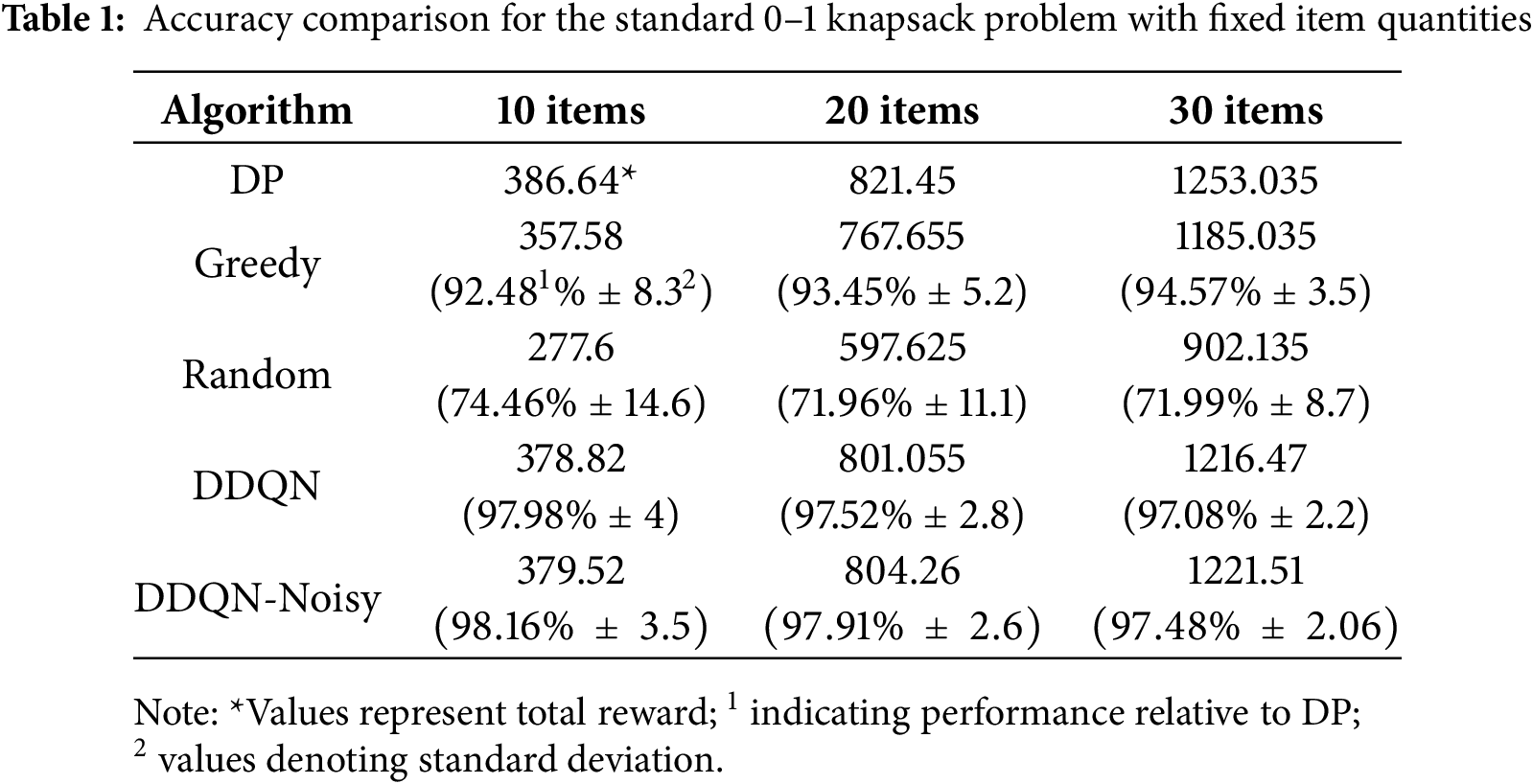
Standard Two-Dimensional Knapsack Problem (0–1 Selection)

Table 1 compares the performance of five different algorithms for the Standard Two-Dimensional Knapsack Problem. It is indicated that DDQN and DDQN-Noisy achieved superior accuracy compared to the Greedy and Random strategies, closely matching the optimal DP solution. DDQN-Noisy consistently attained the smallest standard deviation, demonstrating enhanced robustness over DDQN.

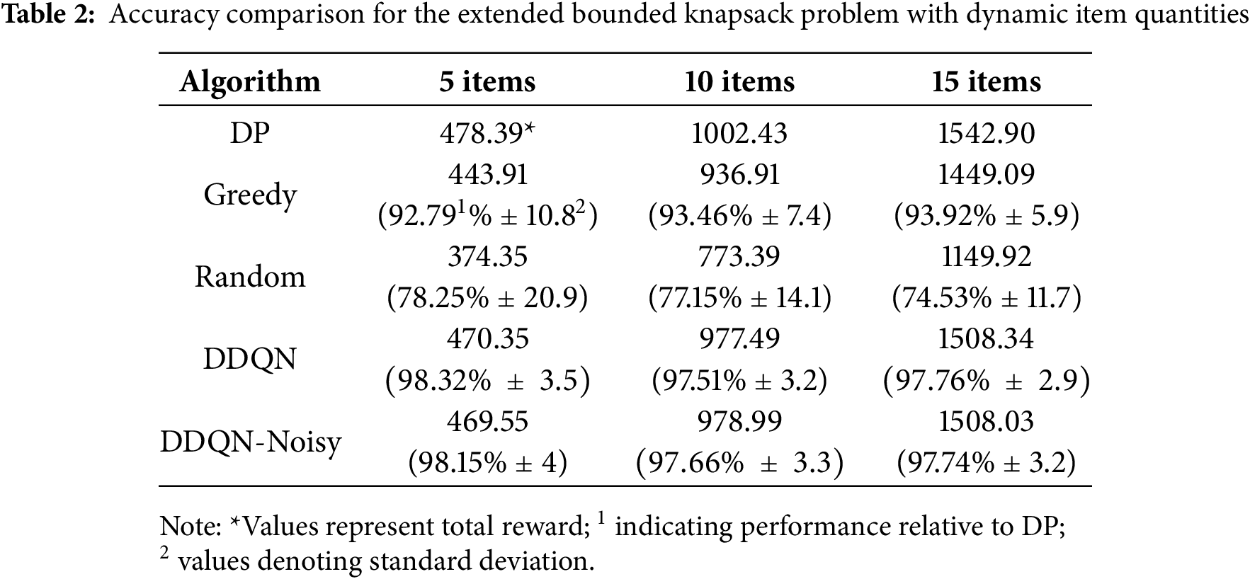
Extended Two-Dimensional Bounded Knapsack (Multi-Quantity Selection)

Table 2 compares the performance of five different algorithms for the Extended Two-Dimensional Bounded Knapsack (Multi-Quantity Selection). We see that in this more complex scenario, DDQN and DDQN-Noisy maintain near-optimal accuracy, outperforming Greedy by 4%–5%, while Random strategies exhibited extreme instability (e.g., 20.9% standard deviation) and low accuracy (77%–78%). The trend reflected in the problem is similar with that in Standard Two-Dimensional Knapsack Problem, which indicates that our algorithms have strong generalizability.

4.2.2 Total Reward Analysis

In this subsection, we focus on Standard two-dimensional knapsack problem. The trend reflected in Extended Two-Dimensional Bounded Knapsack is similar with that in Standard Two-Dimensional Knapsack Problem.

Modified Environment State (Fig. 2a)

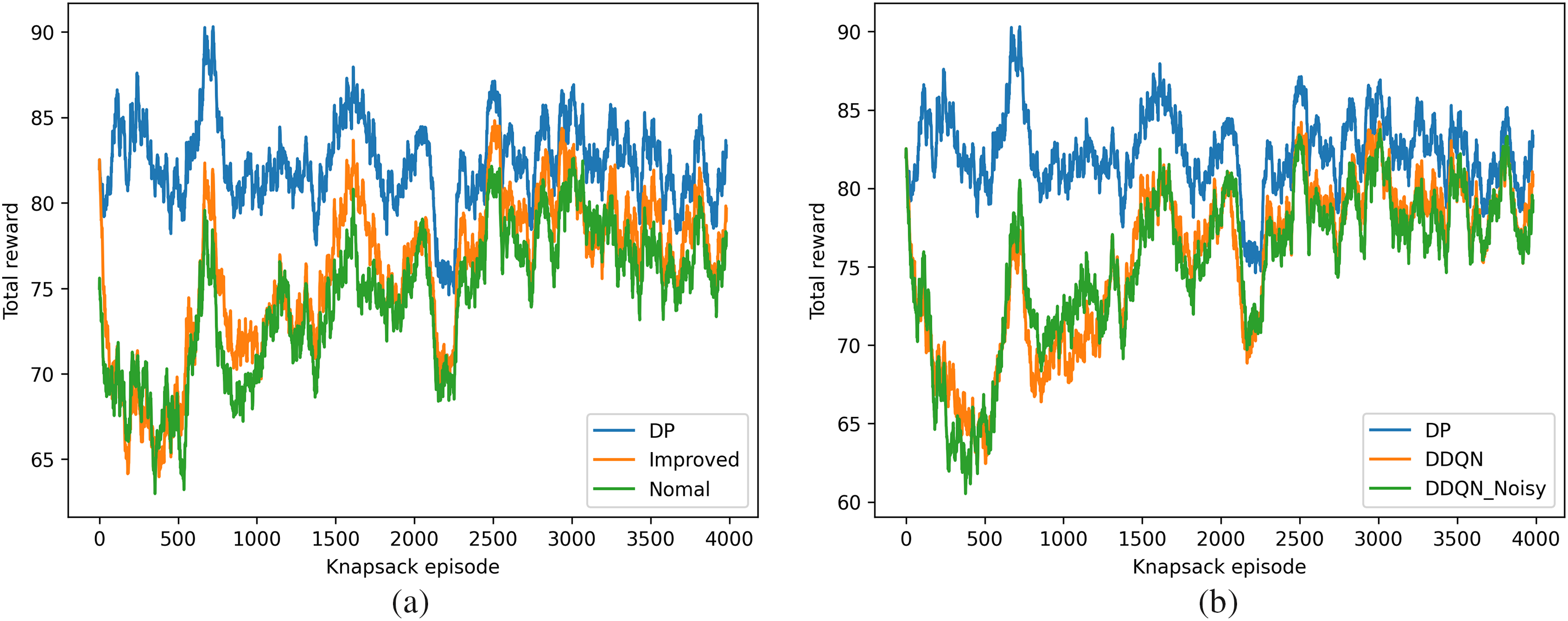
Figure 2: (a) Comparison of total reward during training for DDQN Models with and without environment state modifications over 4000 episodes, showing how such adjustments improve reward accumulation over 4000 training episodes; (b) Comparison of total reward during training for DDQN and DDQN-noisy models in the modified environment over 4000 episodes, illustrating the performance improvement with Noisy layers over 4000 episodes

•      The total reward obtained during training with DDQN was compared before and after modifying the environment state. The modified state improved the training performance significantly, as seen in the increased reward trends over 4000 episodes.

•      The improved DDQN model consistently outperformed the baseline Normal DDQN model across episodes, demonstrating the benefit of state modifications.

Noisy Layers Impact (Fig. 2b)

•      The total reward during training was further analyzed for DDQN and DDQN-Noisy models in the modified environment. DDQN-Noisy consistently achieved slightly higher rewards compared to DDQN alone, highlighting the positive impact of adding noisy layers to the model.

4.2.3 Runtime Efficiency (Fig. 3a,b)

In this subsection, we focus on Standard two-dimensional knapsack problem. The trend reflected in Extended Two-Dimensional Bounded Knapsack is similar with that in Standard Two-Dimensional Knapsack Problem. The runtime of each algorithm was evaluated by varying the number of items in the knapsack. The results indicate the following trends:

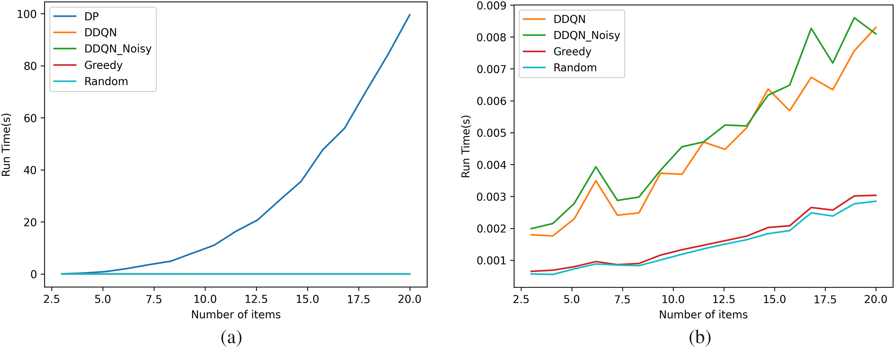
Figure 3: (a) Runtime Comparison of All Algorithms (DP, Greedy, Random, DDQN, and DDQN-Noisy) for Knapsack Problem Instances with Varying Item Quantities; (b) Runtime Comparison of Greedy, Random, DDQN, and DDQN-Noisy (Excluding DP) for Knapsack Problem Instances with Varying Item Quantities

•      DP: Exhibited the highest runtime due to its exhaustive search approach, with exponential growth as the number of items increased.

Runtime without DP (Fig. 3b)

To better visualize the runtime of scalable algorithms, DP was excluded from this analysis. The comparison showed that:

•      Greedy and Random: Achieved the fastest runtimes, as expected, but with lower accuracy.

•      DDQN and DDQN-Noisy: While slightly slower than Greedy and Random, their runtime remained manageable, demonstrating their scalability. DDQN-Noisy was marginally slower than DDQN due to the additional computational overhead of noisy layers.

4.3 Detailed Analysis of Results and Performance Insights

1. DP

DP achieved the highest total value in all three test cases, delivering an optimal solution, as expected. However, its computational complexity makes it impractical for larger problem sizes, particularly when the number of items increases (e.g., with 30 items). While DP provides the best solution, its exponential runtime limits its feasibility for real-time or large-scale applications, highlighting the need for more efficient alternatives.

2. Greedy Algorithm

The Greedy Algorithm, while providing a suboptimal solution, consistently performed 5%–7% worse than DP. Despite this suboptimality, the Greedy algorithm demonstrated efficient performance, with fast execution times. The results show that Greedy is a reasonable choice for smaller problem sizes (10 and 20 items), but as the number of items increases, its performance declines, especially in comparison to more sophisticated methods.

3. Random Selection

Random Selection, as expected, yielded the worst performance, generating solutions that were approximately 25%–30% worse than the Greedy algorithm and 30%–40% worse than DP. This outcome emphasizes the importance of optimization techniques in solving the knapsack problem efficiently, as Random Selection lacks any form of strategy or heuristics to guide its decision-making.

4. DDQN

DDQN, without Noisy layers, demonstrated a significant improvement over both Greedy and Random Selection, achieving a solution that was approximately 97% of the optimal DP value. The DDQN model performed well across all problem sizes, striking a balance between solution quality and training time. This indicates that DDQN can provide near-optimal solutions while avoiding the computational overhead of DP, making it suitable for real-time applications.

5. DDQN-Noisy

The addition of Noisy layers to DDQN further improved performance, with DDQN-Noisy achieving a 0.2%–0.5% increase in the total value across all problem sizes. This subtle yet significant improvement highlights the value of Noisy layers in enhancing the model’s exploration abilities, helping it finds better solutions that would have been missed by a more deterministic model. While the improvements were small, they were consistent, suggesting that Noisy layers fine-tune the agent’s decision-making process, making it more robust to variability in the environment.

Key Findings:

Accuracy: DDQN and DDQN-Noisy achieved near-optimal solutions compared to the DP baseline, outperforming both Greedy and Random Selection. Among them, DDQN-Noisy delivered the most consistent results, as evidenced by its minimal standard deviation across all test cases.

Stability: DDQN-Noisy exhibited superior stability during both the training and testing phases. It showed the lowest standard deviation in total rewards, making it particularly suitable for applications where consistency and reliable performance are crucial.

Runtime Efficiency: While DP was the most accurate, its impractical runtime for larger problems made it unsuitable for many applications. Greedy and Random Selection, although fast, lacked accuracy. DDQN models achieved high accuracy with reasonable computational costs. The slight increase in runtime for DDQN-Noisy compared to DDQN was justified by the improved performance and enhanced stability, making DDQN-Noisy a good trade-off between accuracy and efficiency.

5  Conclusion and Future Work

This paper introduces a novel RL method for solving the KP, overcoming the limitations of traditional approaches such as DP and greedy algorithms. We enhance the state representation by normalizing item weights, volumes, and values, which improves the decision-making capabilities of the RL agent. Our method achieves significant speed enhancements, outperforming DP by over 9000 times. Additionally, by integrating Noisy layers into the RL model, we achieve a performance increase that boosts accuracy by 0.2% to 0.5%, while also stabilizing the learning process.

The proposed RL technique excels in exploring large state and action spaces, adapting to complex scenarios, and delivering near-optimal solutions more efficiently than traditional algorithms. This research presents a promising solution to the scalability and adaptability issues faced by conventional methods.

Future research could investigate further enhancements to the RL framework, such as integrating multi-agent [24] systems to tackle distributed knapsack problems or employing transfer learning [25] to apply learned strategies across different problem instances. Additionally, hybrid approaches that combine RL with other optimization techniques [26]—such as genetic algorithms or dynamic programming—could provide even more powerful solutions for large-scale or time-sensitive applications.

Acknowledgement: We would like to extend our sincere appreciation to the editor and reviewers for their valuable feedback and constructive comments, which greatly improved the quality of this paper.

Funding Statement: This work was supported in part by the Research Start-Up Funds of South-Central Minzu University under Grants YZZ23002, YZY23001, and YZZ18006, in part by the Hubei Provincial Natural Science Foundation of China under Grants 2024AFB842 and 2023AFB202, in part by the Knowledge Innovation Program of Wuhan Basic Research under Grant 2023010201010151, in part by the Spring Sunshine Program of Ministry of Education of the People’s Republic of China under Grant HZKY20220331, and in part by the Funds for Academic Innovation Teams and Research Platform of South-Central Minzu University Grant Number: XT224003, PTZ24001, and in part by the Career Development Fund (CDF) of the Agency for Science, Technology and Research (A*STAR) (Grant Number: C233312007).

Author Contributions: Conceptualization, methodology and validation, Zhenfu Zhang; resources, writing original draft preparation, Haiyan Yin; supervision, writing review and editing, formal analysis, Liudong Zuo, Pan Lai. All authors reviewed the results and approved the final version of the manuscript.

Availability of Data and Materials: Not applicable.

Ethics Approval: Not applicable.

Conflicts of Interest: The authors declare no conflicts of interest to report regarding the present study.

References

1. Kulkarni AJ, Shabir H. Solving 0-1 knapsack problem using cohort intelligence algorithm. Int J Mach Learn Cybern. 2016;7(3):427–41. doi:10.1007/s13042-014-0272-y. [Google Scholar] [CrossRef]

2. Baldo A, Boffa M, Cascioli L, Fadda E, Lanza C, Ravera A. The polynomial robust knapsack problem. Eur J Oper Res. 2023;305(3):1424–34. doi:10.1016/j.ejor.2022.06.029. [Google Scholar] [CrossRef]

3. He Y, Wang J, Liu X, Wang X, Ouyang H. Modeling and solving of knapsack problem with setup based on evolutionary algorithm. Math Comput Simul. 2024;219(9):378–403. doi:10.1016/j.matcom.2023.12.033. [Google Scholar] [CrossRef]

4. Fréville A. The multidimensional 0–1 knapsack problem: an overview. Eur J Oper Res. 2004;155(1):1–21. doi:10.1016/S0377-2217(03)00274-1. [Google Scholar] [CrossRef]

5. LeCun Y, Bengio Y, Hinton G. Deep learning. Nature. 2015;521(7553):436–44. doi:10.1038/nature14539. [Google Scholar] [PubMed] [CrossRef]

6. Sutton RS, Barto AG. Reinforcement learning: an introduction. Cambridge, MA, USA: MIT Press; 2018. [Google Scholar]

7. Ernst D, Louette A, Feuerriegel S, Hartmann J, Janiesch C, Zschech P. Introduction to reinforcement learning. Liège, Belgium: ULiège; 2024. p. 111–26. [Google Scholar]

8. Mnih V, Kavukcuoglu K, Silver D, Rusu AA, Veness J, Bellemare MG, et al. Human-level control through deep reinforcement learning. Nature. 2015;518(7540):529–33. doi:10.1038/nature14236. [Google Scholar] [PubMed] [CrossRef]

9. Silver D, Huang A, Maddison CJ, Guez A, Sifre L, van den Driessche G, et al. Mastering the game of Go with deep neural networks and tree search. Nature. 2016;529(7587):484–9. doi:10.1038/nature16961. [Google Scholar] [PubMed] [CrossRef]

10. Legg S, Hutter M. Universal intelligence: a definition of machine intelligence. Mines Mach. 2007;17(4):391–444. doi:10.1007/s11023-007-9079-x. [Google Scholar] [CrossRef]

11. Yildiz B. Reinforcement learning using fully connected, attention, and transformer models in knapsack problem solving. Concurr Comput. 2022;34(9):e6509. doi:10.1002/cpe.6509. [Google Scholar] [CrossRef]

12. Martello S, Toth P. Algorithms for knapsack problems. In: North-holland mathematics studies. Amsterdam, The Netherlands: Elsevier; 1987. p. 213–57. [Google Scholar]

13. Kosuch S, Lisser A. On two-stage stochastic knapsack problems. Discrete Appl Math. 2011;159(16):1827–41. doi:10.1016/j.dam.2010.04.006. [Google Scholar] [CrossRef]

14. Chu P, Beasley J. A genetic algorithm for the multidimensional knapsack problem. J Heuristics. 1998;4(1):63–86. [Google Scholar]

15. Sahni S. Approximate algorithms for the 0/1 knapsack problem. J ACM. 1975;22(1):115–24. doi:10.1145/321864.321873. [Google Scholar] [CrossRef]

16. Bello I, Pham H, Le QV, Norouzi M, Bengio S. Neural combinatorial optimization with reinforcement learning. arXiv:1611.09940. 2016. [Google Scholar]

17. Nazari M, Oroojlooy A, Snyder L, Takác M. Reinforcement learning for solving the vehicle routing problem. In: Advances in Neural Information Processing Systems; 2018 Dec 3–8; Montréal, QC, Canada. [Google Scholar]

18. Dai H, Khalil E, Zhang Y, Dilkina B, Song L. Learning combinatorial optimization algorithms over graphs. In: Advances in Neural Information Processing Systems; 2017 Dec 4–9; Long Beach, CA, USA. [Google Scholar]

19. Parisotto E, Song F, Rae J, Pascanu R, Gulcehre C, Jayakumar S, et al. Stabilizing transformers for reinforcement learning. In: Proceedings of the 37th International Conference on Machine Learning; 2020 Jul 13–18; Online. [Google Scholar]

20. Gu S, Hao T. A pointer network based deep learning algorithm for 0–1 Knapsack Problem. In: 2018 Tenth International Conference on Advanced Computational Intelligence (ICACI); 2018 Mar 29–31; Xiamen, China. doi:10.1109/ICACI.2018.8377505. [Google Scholar] [CrossRef]

21. Denysiuk R, Gaspar-Cunha A, Delbem ACB. Neuroevolution for solving multiobjective knapsack problems. Expert Syst Appl. 2019;116(12):65–77. doi:10.1016/j.eswa.2018.09.004. [Google Scholar] [CrossRef]

22. Fortunato M, Azar MG, Piot B, Menick J, Osband I, Graves A, et al. Noisy networks for exploration. In: International Conference on Learning Representations; 2018 Apr 30–May 3; Vancouver, BC, Canada. [Google Scholar]

23. Wang Z, Schaul T, Hessel M, Hasselt H, Lanctot M, Freitas N. Dueling network architectures for deep reinforcement learning. In: International Conference on Machine Learning; 2016 Jun 19–4; New York City, NY, USA. p. 1995–2003. [Google Scholar]

24. Zhang K, Yang Z, Başar T. Multi-agent reinforcement learning: a selective overview of theories and algorithms. In: Handbook of reinforcement learning and control. Berlin/Heidelberg, Germany: Springer; 2021. p. 321–84. [Google Scholar]

25. Zhu Z, Lin K, Jain AK, Zhou J. Transfer learning in deep reinforcement learning: a survey. IEEE Trans Pattern Anal Mach Intell. 2023;45(11):13344–62. doi:10.1109/TPAMI.2023.3292075. [Google Scholar] [PubMed] [CrossRef]

26. Zheng J, He K, Zhou J, Jin Y, Li CM. Combining reinforcement learning with Lin-kernighan-helsgaun algorithm for the traveling salesman problem. Proc AAAI Conf Artif Intell. 2021;35(14):12445–52. doi:10.1609/aaai.v35i14.17476. [Google Scholar] [CrossRef]