
 Submit a Paper
 Propose a Special lssue
 Open Access
ARTICLE
Unsupervised Anomaly Detection in Time Series Data via Enhanced VAE-Transformer Framework
1 Institute of Hydrogeology and Environmental Geology, Chinese Academy of Geological Sciences, Shijiazhuang, 050061, China
2 Hebei Provincial Engineering Research Center for Supply Chain Big Data Analytics & Data Security, Shijiazhuang, 050024, China
3 College of Computer and Cyber Security, Hebei Normal University, Shijiazhuang, 050024, China
* Corresponding Author: Bin Xie. Email:
Computers, Materials & Continua 2025, 84(1), 843-860. https://doi.org/10.32604/cmc.2025.063151
Received 06 January 2025; Accepted 27 March 2025; Issue published 09 June 2025
 View Full Text
 Download PDF
Abstract
Time series anomaly detection is crucial in finance, healthcare, and industrial monitoring. However, traditional methods often face challenges when handling time series data, such as limited feature extraction capability, poor temporal dependency handling, and suboptimal real-time performance, sometimes even neglecting the temporal relationships between data. To address these issues and improve anomaly detection performance by better capturing temporal dependencies, we propose an unsupervised time series anomaly detection method, VLT-Anomaly. First, we enhance the Variational Autoencoder (VAE) module by redesigning its network structure to better suit anomaly detection through data reconstruction. We introduce hyperparameters to control the weight of the Kullback-Leibler (KL) divergence term in the Evidence Lower Bound (ELBO), thereby improving the encoder module’s decoupling and expressive power in the latent space, which yields more effective latent representations of the data. Next, we incorporate transformer and Long Short-Term Memory (LSTM) modules to estimate the long-term dependencies of the latent representations, capturing both forward and backward temporal relationships and performing time series forecasting. Finally, we compute the reconstruction error by averaging the predicted results and decoder reconstruction and detect anomalies through grid search for optimal threshold values. Experimental results demonstrate that the proposed method performs superior anomaly detection on multiple public time series datasets, effectively extracting complex time-related features and enabling efficient computation and real-time anomaly detection. It improves detection accuracy and robustness while reducing false positives and false negatives.Keywords
Time series data is widely present in various fields such as financial markets [1–3], healthcare monitoring [4,5], industrial process control [6], and geological disaster early warning [7]. Effective anomaly detection in time series can help identify potential issues and predict system failures, thereby improving system reliability and safety. However, time series data often exhibits complexity and diversity, which poses significant challenges for anomaly detection [8,9].
Researchers have explored anomaly detection methods from different perspectives in response to these challenges. Among them, unsupervised anomaly detection methods do not rely on labeled data; instead, anomalies are detected by learning the normal patterns of the data [10]. Unlike supervised learning methods, unsupervised learning is more versatile and especially suited for real-world applications where labeled data is often scarce [11]. Standard unsupervised anomaly detection methods include statistical, machine learning, and deep learning approaches.
Traditional anomaly detection methods have several limitations when handling complex time series data [12]. For example, statistical methods [13] depend on the statistical properties of the data but suffer from strong assumptions, complex parameter selection, limited ability to handle non-linear patterns, and poor performance in dealing with long-term dependencies and changing data patterns. Machine learning-based methods [14] are less automated, requiring manual feature engineering and parameter tuning.
With the rapid development of artificial intelligence in computer science, deep learning methods [15,16] have gradually shown advantages in anomaly detection. Studies by He et al. [17] demonstrate that regarding anomaly detection performance, deep learning methods outperform traditional machine learning techniques, such as principal component analysis, clustering, support vector machine, frequent pattern mining, and graph mining. However, there is still room for improvement in feature extraction, anomaly detection capabilities, time series context information utilization, and model robustness. For instance, autoencoder [18] can identify anomalies by compressing and reconstructing data, but they often struggle to capture the temporal dependencies inherent in time series data. Recurrent Neural Networks (RNN), particularly Long Short-Term Memory (LSTM) networks [19] and Gated Recurrent Units (GRU) [20], are adept at handling sequential data but often require large amounts of labeled data for training in anomaly detection tasks. Zamanzadeh et al. [21] proposed the LSTM-AD algorithm, utilizing LSTM networks to address anomaly detection in time series data. However, the method has limitations in capturing multi-scale temporal features, lacks the ability to model complex data distributions, and exhibits weak generalization capability when confronted with large-scale and diverse anomaly patterns. Variational Autoencoders (VAE) [22], which learn the probabilistic distribution of the data for reconstruction and generation, are limited in their ability to capture temporal dependencies and complex dynamic changes in time series data. In recent years, RNN have often been combined with VAE and Generative Adversarial Networks (GAN) to detect multivariate time series anomalies.
Despite the aforementioned performance improvements, the models still face several critical challenges [23]. First, the training process remains susceptible to data uncertainties and anomalous patterns, potentially inducing overfitting issues that undermine their generalization capability. Notably, in time series anomaly detection, the dearth of effective data augmentation techniques restricts the model’s capacity to comprehensively learn normal patterns while accommodating the diversity and unpredictability of anomalous data. This limitation renders the model prone to overfitting on training datasets, consequently impairing its detection performance when encountering novel anomaly patterns unseen during training. Such performance degradation manifests particularly in scenarios requiring robust generalization to evolving anomaly types and temporal variations. To overcome the limitations of existing methods, we propose an unsupervised anomaly detection approach for time series data, combining
1. We use an improved
2. We employ a transformer model to process the low-dimensional embeddings generated by the encoder, manage long-term sequence patterns, and predict the latent representations. We further leverage bidirectional LSTM (BiLSTM) to fully utilize both forward and backward information fully, improving the model’s ability to capture time series dependencies.
3. We input the transformer’s prediction results into the improved
The prediction module’s main advantage is its ability to handle long-range dependencies and local context information efficiently. The transformer provides strong global information capture and supports parallel computation, making it well-suited for long sequence data. The BiLSTM enhances the model’s ability to perform bidirectional modeling of time series data. Combining these two models improves the model’s representation ability and training efficiency and significantly enhances information flow and stability, resulting in superior performance on complex time series tasks.
With the rapid advancement of artificial intelligence in computer science, deep learning methods have increasingly demonstrated significant advantages in anomaly detection. Experts have started focusing on the research of time series anomaly detection algorithms. Among these, variational autoencoders (VAEs) have become a primary research subject due to their ability to learn the probabilistic distribution of data for reconstruction and generation. As a powerful generative model, VAE combines the strengths of deep learning and probabilistic modeling, enabling it to effectively handle complex data distributions by learning the latent representations of the data. This makes VAE a promising approach for anomaly detection tasks. However, the aforementioned mathematical principles of VAE require modifications in specific applications. For example, in creative generation tasks, high creativity in generated samples is required, while in anomaly detection, the completeness of generated samples may be less critical, and it is often desirable to disregard noisy data points. Despite VAE’s success in generative modeling and unsupervised learning, it still has limitations in learning disentangled representations of the latent space [24]. The feedforward neural network in VAE assumes that data at each time point is independent, and the network’s output only depends on the current input. However, time series data exhibits important temporal dependencies. Therefore, it is necessary to incorporate network structures into the VAE encoder and decoder to account for these temporal dependencies. How to design appropriate encoder and decoder network structures for specific application scenarios is an area that warrants further exploration. Fan et al. [25] introduced federated learning and VAE for anomaly detection, improving model collaboration and privacy protection. However, these models still struggle to capture time dependencies and dynamic changes, resulting in suboptimal performance for time-dependent anomaly detection tasks.
In recent years, RNN have often been combined with VAE and GAN to detect multivariate time series anomalies. RNN such as LSTM and GRU are commonly used as base models in VAE and GAN to capture temporal dependencies in multivariate time series. VAE and GAN can jointly learn the dependencies across feature dimensions and the complex distribution across time dimensions. As two standard generative models, VAE and GAN focus on learning the rules or distributions of data generation. Thus, to better describe and model the data, it is necessary to represent the implicit features of multivariate time series data. Both methods utilize random noise during data generation and measure the discrepancy between the noise and the training data distribution, though their modeling principles and training methods differ. Lin et al. [26] enhanced the temporal dependency handling of the VAE model by combining it with RNN, improving its performance in anomaly detection. Chen et al. [27] proposed a semi-supervised VAE-based anomaly detection strategy (LR-SemiVAE) using LSTM. The model leverages VAE for feature dimensionality reduction and multivariate time series data reconstruction, judging anomalies based on reconstruction probability scores. However, this model requires accurate labels for training, limiting its applicability. Chen et al. [28] proposed an LSTM-GAN-based time series anomaly detection model. However, GAN-based approaches require identifying the best mapping from real-time to latent space during anomaly detection, introducing new errors and requiring longer computation time. Song et al. [29] proposed the VAE-Transformer model by combining Variational Autoencoders (VAE) for short-term local anomaly detection and Transformer for long-term trend analysis. The model is capable of capturing immediate anomalies and broader temporal patterns. However, it still faces limitations in capturing bidirectional dependencies, stronger long-term dependencies, and multi-level anomaly detection capabilities. Furthermore, the model’s ability to better understand the interactions between past and future in time series, as well as handle complex scenarios influenced by both future trends and past patterns, remains inadequate. He et al. [30] proposed a novel unsupervised anomaly detection method for multivariate time series, named VAEAT, which uses VAEs as the main architecture and creates a two-phase training strategy using the adversarial training idea. This method not only solves the problem that VAE fails to adequately learn the underlying data distribution, but also enhances its noise resistance. However, this paper does not thoroughly explore the relationship between time series attributes for detecting overall abnormalities through anomalies at a single attribute.
To overcome the limitations of existing methods, we propose an unsupervised anomaly detection approach for time series data, combining
Given a time series
The overall framework of the proposed method consists of two key modules: the
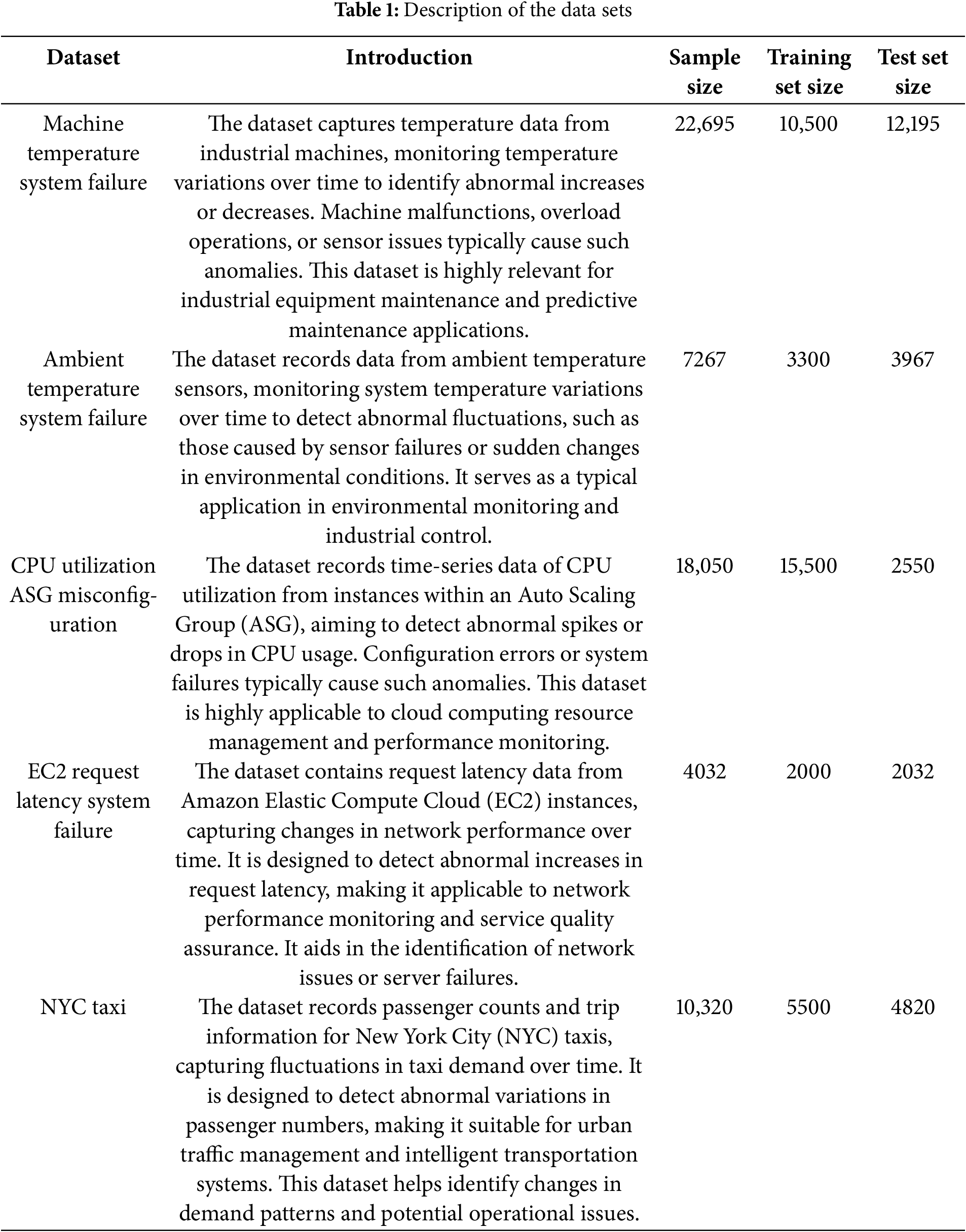
The dataset used in this study is the NAB (Numenta Anomaly Benchmark) dataset. The NAB dataset is a benchmark specifically designed for evaluating the performance of time series anomaly detection algorithms. Numenta released it to provide a standardized data set to enable researchers to fairly and objectively compare different anomaly detection methods [31]. To assess the generalization capability of the algorithm, the selected dataset covers a range of time series data, including industrial machine temperatures, environmental temperatures, CPU utilization, network request latency, and taxi demand [32]. Table 1 provides a detailed description of the datasets used, as well as the division of the training and testing sets in this experiment.
(a) Data Normalization: Data normalization is performed by standardizing all data using the mean and standard deviation of the training set. The data is normalized to follow a standard normal distribution with a mean of 0 and a standard deviation of (1):
where
(b) Training and Testing Set Separation: The training and testing sets are separated from the given time series to train the model unsupervised. Fig. 1 illustrates the separation process: Continuous time series without anomalies are selected as the training data, and the remaining time series containing anomalies are used as the testing data for model evaluation.
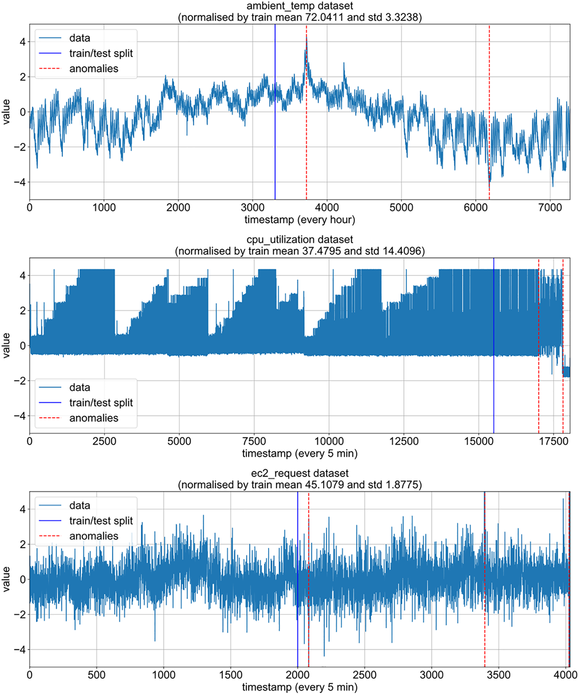
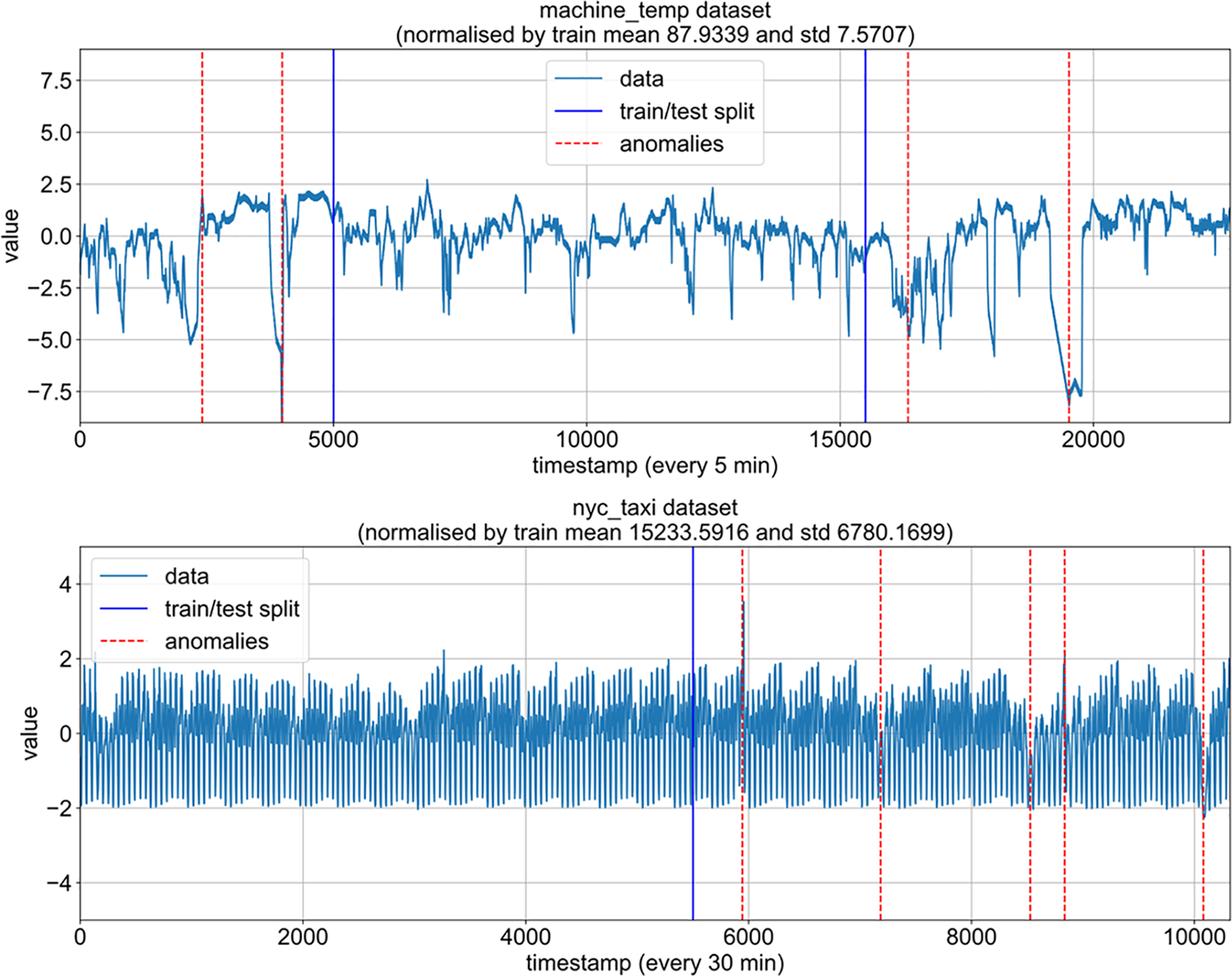
Figure 1: Training-test set separation
(c) Dataset Partition and Augmentation: Ten percent of the data from the training set is extracted as a validation set, which is completely separate from the training set for model validation and debugging. In the
The sliding window at time
This method effectively increases the number of training windows, which helps improve the model’s generalization ability and enhances the performance of the anomaly detection model in practical applications.
In the training set of the transformer model, both sliding window and non-overlapping window methods are applied to generate multiple training sequences from the time series data. The specific steps are as follows:
(a) Generate Non-Overlapping Windows: First, fixed-length, non-overlapping windows are generated based on the sliding window size and the number of training samples. The number of non-overlapping windows is:
where
(b) Generate Transformer Input Sequences: Then, the input sequences for the transformer are generated. For each starting offset
where
(c) Combine All Sequences: All the generated transformer sequences are then combined into a complete training sequence set, with the total number of sequences given by:
which simplifies to:
where the
By effectively utilizing the sliding window and non-overlapping window techniques and continuously adjusting the starting offset of the window, a large number of transformer input sequences are generated, which significantly increases the number of training sequences and enhances the model’s robustness and generalization capability.
3.2 Model Introduction and Training
The
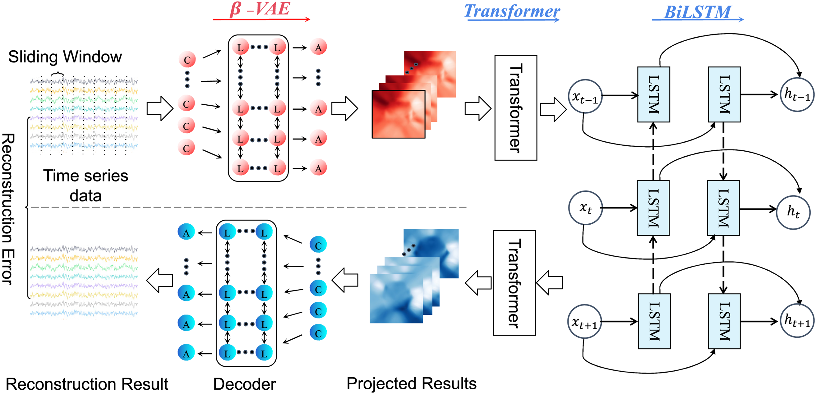
Figure 2: Anomaly detection process diagram
The decoder receives the encoded feature vector or a randomly sampled latent vector as input and reconstructs the original signal. Depending on the input window length, the decoder structure is adjusted accordingly, employing deconvolution and transposed convolution operations for the stepwise reconstruction of the window. The final output is the reconstructed signal data with shape
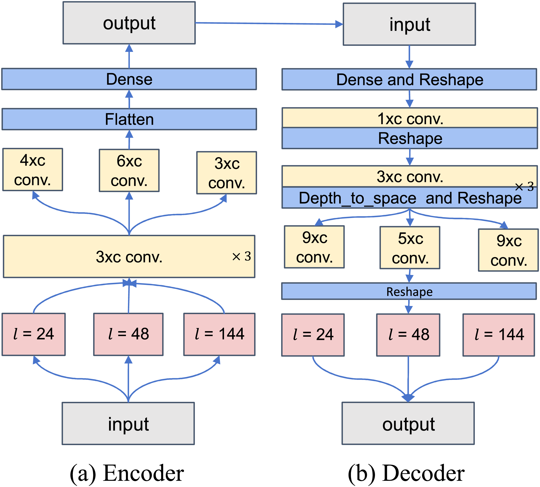
Figure 3:
During the training phase, the
The model iterates through the training dataset to maximize the ELBO loss and further optimize the parameters of the
After the
The Eq. (8) represents the window sequence starting at time
The
Transformer module consists of transformer model and BiLSTM model. The BiLSTM model parameters are optimized by minimizing the prediction error of the final embedding:
Since the method in this paper is an unsupervised anomaly detection approach, all parameters of the
3.3 Anomaly Detection Using VLT-Anomaly Models
After training, the VLT-Anomaly model can be applied for both offline anomaly detection and real-time anomaly detection, and estimate anomalous regions. The model uses the test sequence
where
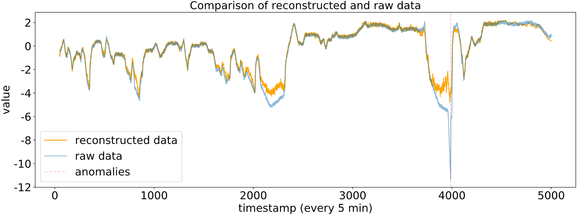
Figure 4: Comparison of reconstructed and raw data
For the reconstructed windows, a scoring function
To detect anomalies, a threshold
When sufficient data is available, a validation set containing normal and anomalous samples should be used to determine
3.4 Advantages of the VLT-Anomaly
The VLT-Anomaly framework integrates
To address the limitations of traditional VAE-LSTM methods in terms of reconstruction error sensitivity and latent space prediction accuracy, VLT-Anomaly adopts a modular design that decouples the transformer and BiLSTM components for independent optimization. This modular approach allows for flexible adjustments to the number of transformer layers, attention heads, and BiLSTM hidden units, making the framework adaptable to diverse task requirements. Additionally, techniques such as a learning rate scheduler and dropout are employed to accelerate convergence and prevent overfitting, enhancing the overall robustness of the model. Regarding loss design, VLT-Anomaly employs a multi-objective optimization strategy that balances KL divergence, latent space prediction error, and reconstruction error through a weighted combination, ensuring both stability and detection precision.
In summary, by seamlessly integrating global and local feature modeling, efficient parallel computation, and modular optimization flexibility, VLT-Anomaly provides an efficient, accurate, and robust solution for anomaly detection in complex time series data, establishing itself as a significant improvement over traditional methods.
4 Analysis of Experimental Results
Precision, recall, and F1 score are used as evaluation metrics for anomaly detection. Specifically, precision represents the proportion of correctly predicted anomalies among all predicted anomalies, while recall indicates the proportion of correctly predicted anomalies among all true anomalies. The F1 score is a balanced metric that considers both precision and recall. In the subsequent sections, precision is denoted as P, recall as R, and F1 score as F1, with their respective formulas shown in Eqs. (15)–(17):
where TP (True Positives) refers to the number of correctly predicted anomalies, FP (False Positives) refers to the number of normal samples incorrectly predicted as anomalies, and FN (False Negatives) refers to the number of anomalies incorrectly predicted as normal.
To validate the effectiveness of the VLT-Anomaly model, the experimental process includes two parts: a comparative experiment with other similar methods, and an ablation study on key modules. In the comparative experiment, the number of sliding windows in the sequence
The experiment uses the TensorFlow deep learning framework, with Python 3.6 as the programming language. The development environment is set up with Anaconda (WSL2), and JetBrains PyCharm 2024.1 Professional Edition is used for development. The workstation runs on Windows 11 Professional (64-bit), with hardware configurations including 32 GB of memory, an Intel Core i9-14900 HX (2.20 GHz) processor, and an NVIDIA GeForce RTX 4060 GPU.
The proposed VLT-Anomaly algorithm was evaluated on five real-world time series datasets containing actual anomalous events: Ambient Temperature, CPU Utilization AWS, CPU Utilization EC2 (from Amazon East Coast Data Center servers), Machine Temperature (industrial machinery), and NYC Taxi Passenger Count [31]. The algorithm was compared with six commonly used time series anomaly detection algorithms: VAE [22], LSTM-AD [21], ARMA [26], VAE-LSTM [33], LR-SemiVAE [27], LSTM-GAN [28], VAE-Transformer [29], and VAEAT [30]. Table 2 presents the experimental results along with the sliding window lengths. The evaluation metrics include Precision, Recall, and F1 Score, all calculated at the threshold that yields the best F1 score.
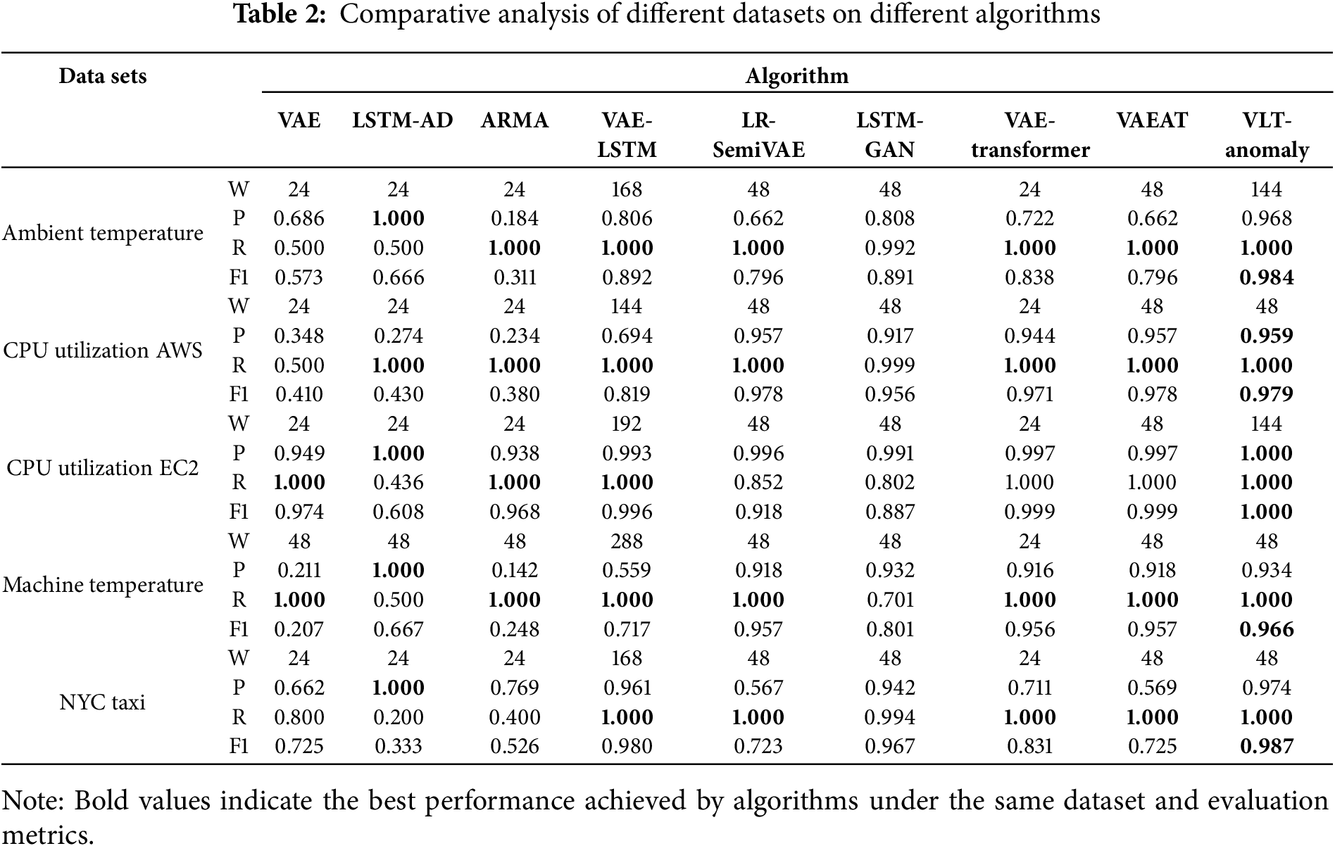
The LSTM-AD method achieved high precision on most datasets but exhibited low recall, indicating that many true anomalies were missed while detected anomalies were accurate. In contrast, VAE demonstrated good recall but lower precision, suggesting a high number of false positives.
The proposed VLT-Anomaly algorithm achieved 100% recall across all datasets, indicating that no anomalies were missed and that all types of anomalies were successfully detected. On all five datasets, the proposed algorithm outperforms the other eight algorithms in terms of F1 score, achieving the best performance. The precision also reaches the best or second-best level across these datasets. The significant improvement in precision indicates a lower false positive rate. The model effectively captured key features of the signals, demonstrated strong reconstruction performance, and achieved efficient representation in the latent space. It outperformed the baseline methods with substantial precision, recall, and F1 score improvements. Overall, the proposed algorithm demonstrates superior performance across all metrics compared to the other baseline algorithms. Fig. 5 provides a more intuitive visualization of the comparison experimental results.
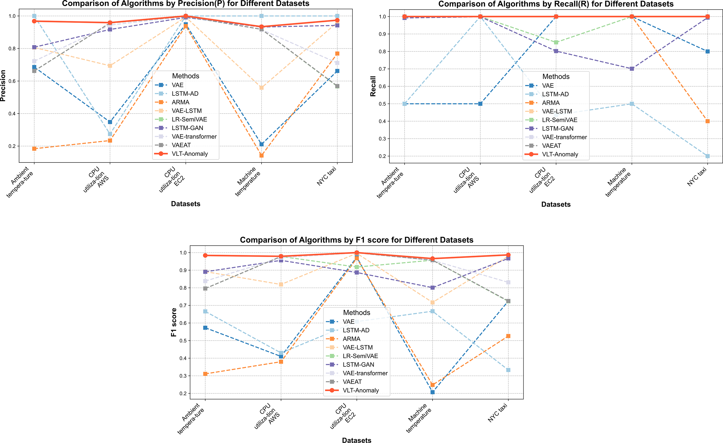
Figure 5: Comparison of algorithms by evaluation metrics for different datasets
To further verify the effectiveness of each improved module, the VAE algorithm and its four variants are used in this section: (1) VAE algorithm. This algorithm only contains the standard VAE algorithm and has the function of data reconstruction. (2) VAE-A algorithm. Based on the VAE algorithm, the LSTM algorithm is introduced to predict the coding results of the VAE encoder, and the processing and memory ability of long time series, namely VAE-LSTM, is considered. (3) VAE-B algorithm. Based on the VAE-LSTM algorithm, the results of forward and reverse bidirectional time series prediction are fused to enhance further the processing and memory function of long time series, namely VAE-BiLSTM. (4) VAE-C algorithm. Based on the VAE-LSTM algorithm, the super parameter
The results of the VAE algorithm and four variants of the algorithm are shown in Table 3. The experimental results show that VAE-A has significantly improved compared with VAE as a whole, mainly because VAE-A introduces the network structure LSTM considering time series. Based on VAE-A, VAE-B effectively improves the detection ability of the model by combining the forward and reverse time series prediction results and fusing them. From the experimental results of the three indicators, 10 of the 15 comparisons have been further improved or equivalent, which verifies the effectiveness of this part of the improvement. Based on VAE-A, VAE-C retains the framework of the original VAE model, redesigns its internal network to make it more suitable for anomaly detection, and introduces the hyperparameter
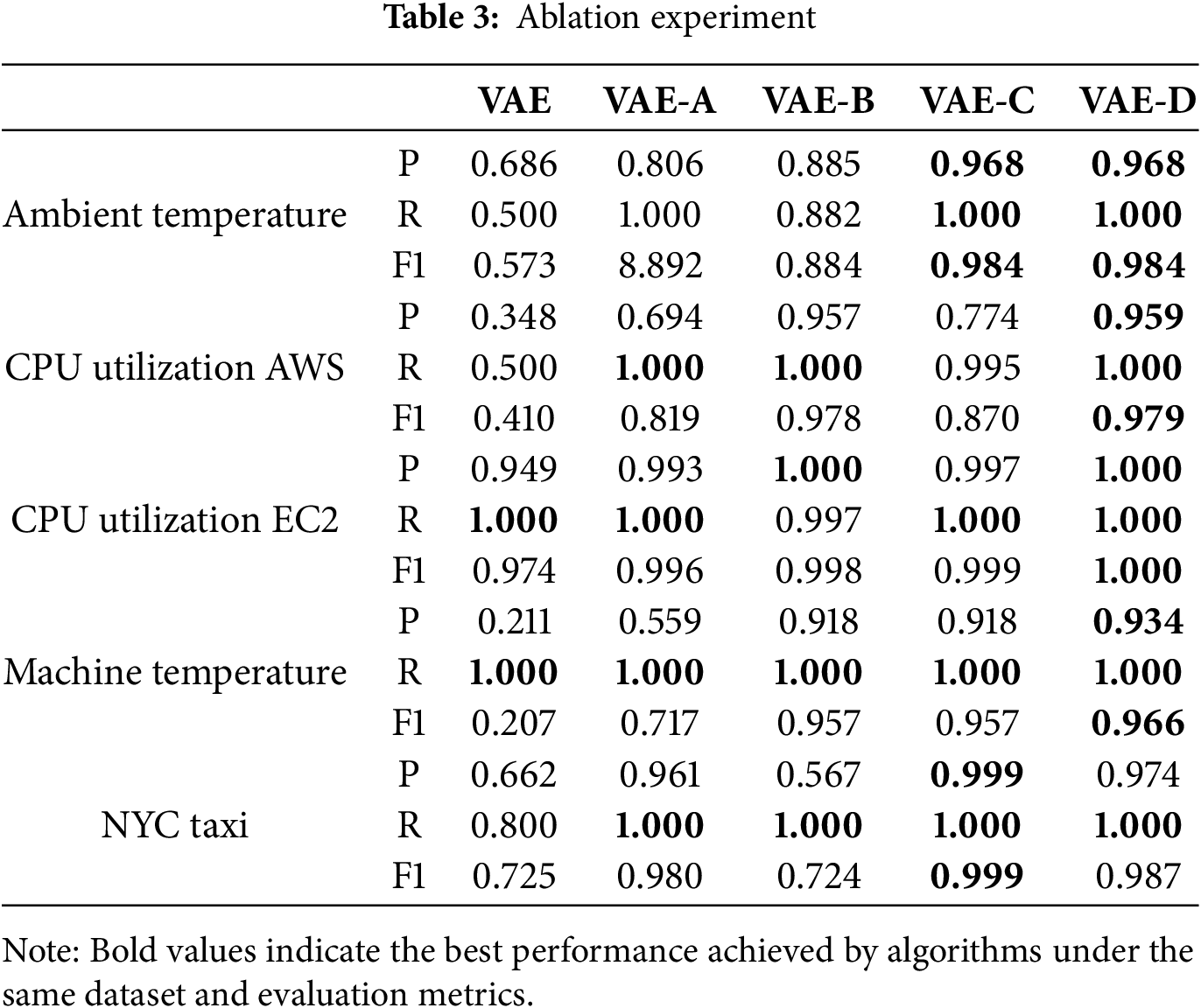
The detection effect of VAE-D algorithm is further improved compared with VAE-B or VAE-C. Even compared with the VAE-A algorithm and the VAE algorithm, the best results were obtained in 15 comparisons. Generally, this study uses VAE to reduce the feature dimension and reconstruct the time series data. In addition, the transformer and BiLSTM are integrated into the encoder and decoder of VAE, and then the abnormal state of the entity is recognized based on the reconstruction error score. The model can capture the time dependence of time series data more effectively. These improvements not only enhance the model’s performance, but also verify the effectiveness of the proposed algorithm.
This study introduces VLT-Anomaly, a novel unsupervised anomaly detection framework designed to address the challenges of time series data, including its inherent diversity, complex temporal dependencies, and the scarcity of labeled data. By integrating
In practice, the VLT-Anomaly framework demonstrates excellent adaptability to a variety of time series scenarios, supported by preprocessing techniques such as data augmentation to enhance performance on datasets with limited sample sizes. The method achieves accurate anomaly detection and localization by optimizing the reconstruction error threshold using grid search, enabling offline and real-time applications. Experimental results confirm the effectiveness of VLT-Anomaly across diverse datasets, where it not only detects anomalies with high precision but also adapts seamlessly to different types of time series data, offering robust solutions for real-time monitoring and historical anomaly mining. However, the study also reveals certain limitations inherent to deep learning models, including challenges in model interpretability and the complexity of hyperparameter tuning, both of which stem from the sophisticated structure of the proposed framework.
There are several promising directions for future work. First, improving the interpretability of the framework is essential. Additionally, automated hyperparameter optimization techniques, such as Bayesian optimization or grid search, could alleviate the difficulties of tuning the framework’s parameters and further improve its usability. Moreover, testing the generalization capabilities of VLT-Anomaly on real-world time series data, particularly from production environments, is another critical step to refining its performance. Real-world data often introduces additional challenges, such as noise and domain-specific constraints, which the framework must address to ensure its robustness and reliability.
Another important direction is extending the framework to handle multi-modal and high-dimensional time series data offers exciting potential for anomaly detection in complex systems. Many real-world scenarios involve multi-source data, such as sensor readings, logs, and images, requiring the framework to integrate and process diverse data streams effectively.
Acknowledgement: The authors thank the editor and anonymous reviewers for their helpful comments and valuable suggestions.
Funding Statement: The authors would appreciate support from the Fundamental Research Funds for Central Public Welfare Research Institutes (SK202324), the Central Guidance on Local Science and Technology Development Fund of Hebei Province (236Z0104G), the National Natural Science Foundation of China (62476078) and the Geological Survey Project of China Geological Survey (G202304-2).
Author Contributions: Study conception and design: Bin Xie, Zhibin Huo; data collection: Chunhao Zhang; analysis and interpretation of results: Chunhao Zhang; draft manuscript preparation: Bin Xie, Chunhao Zhang. All authors reviewed the results and approved the final version of the manuscript.
Availability of Data and Materials: The data that support the findings of this study are openly available in NAB at https://github.com/numenta/NAB (accessed on 1 January 2025).
Ethics Approval: Not applicable.
Conflicts of Interest: The authors declare no conflicts of interest to report regarding the present study.
References
1. Bai L, Cui L, Zhang Z, Xu L, Wang Y, Hancock ER. Entropic dynamic time warping kernels for co-evolving financial time series analysis. IEEE Trans Neural Netw Learn Syst. 2023;34(4):1808–22. doi:10.1109/TNNLS.2020.3006738. [Google Scholar] [PubMed] [CrossRef]
2. Cao FF, Guo XT. Automated financial time series anomaly detection via curiosity-guided exploration and self-imitation learning. Eng Appl Artif Intell. 2024;135(3):108663. doi:10.1016/j.engappai.2024.108663. [Google Scholar] [CrossRef]
3. Hilal W, Gadsden SA, Yawney J. Financial fraud: a review of anomaly detection techniques and recent advances. Expert Syst Appl. 2022;193(8):116429. doi:10.1016/j.eswa.2021.116429. [Google Scholar] [CrossRef]
4. Wang J, Jin H, Chen J, Tan J, Zhong K. Anomaly detection in internet of medical things with blockchain from the perspective of deep neural network. Inf Sci. 2022;617(2):133–49. doi:10.1016/j.ins.2022.10.060. [Google Scholar] [CrossRef]
5. Pinaya WH, Tudosiu PD, Gray R, Rees G, Nachev P, Ourselin S, et al. Unsupervised brain imaging 3D anomaly detection and segmentation with transformers. Med Image Anal. 2022;79:102475. doi:10.1016/j.media.2022.102475. [Google Scholar] [PubMed] [CrossRef]
6. Leng J, Lin Z, Zhou M, Liu Q, Zheng P, Liu Z, et al. Multi-layer parallel transformer model for detecting product quality issues and locating anomalies based on multiple time-series process data in Industry 4.0. J Manuf Syst. 2023;70(7):501–13. doi:10.1016/j.jmsy.2023.08.013. [Google Scholar] [CrossRef]
7. Shi H, Guo J, Deng Y, Qin Z. Machine learning-based anomaly detection of groundwater microdynamics: case study of Chengdu. China Sci Rep. 2023;13(1):14718. doi:10.1038/s41598-023-38447-5. [Google Scholar] [PubMed] [CrossRef]
8. Jin F, Wu H, Liu Y, Zhao J, Wang W. Varying-scale HCA-DBSCAN-based anomaly detection method for multi-dimensional energy data in steel industry. Inf Sci. 2023;647(8):119479. doi:10.1016/j.ins.2023.119479. [Google Scholar] [CrossRef]
9. Lee D, Malacarne S, Aune E. Explainable time series anomaly detection using masked latent generative modeling. Pattern Recognit. 2024;156(3):110826. doi:10.1016/j.patcog.2024.110826. [Google Scholar] [CrossRef]
10. He S, Deng T, Chen B, Wang J. Unsupervised log anomaly detection method based on multi-feature. Comput Mater Contin. 2023;76(1):517–41. doi:10.32604/cmc.2023.037392. [Google Scholar] [CrossRef]
11. Zhao T, Jin L, Zhou X, Li S, Liu S, Zhu J. Unsupervised anomaly detection approach based on adversarial memory autoencoders for multivariate time series. Comput Mater Contin. 2023;76(1):329–46. doi:10.32604/cmc.2023.038595. [Google Scholar] [CrossRef]
12. Audibert J, Michiardi P, Guyard F, Marti S, Zuluaga MA. Do deep neural networks contribute to multivariate time series anomaly detection? Pattern Recognit. 2022;132(3):108945. doi:10.1016/j.patcog.2022.108945. [Google Scholar] [CrossRef]
13. Jeong J, Park E, Han WS, Kim K, Choung S, Chung IM. Identifying outliers of non-Gaussian groundwater state data based on ensemble estimation for long-term trends. J Hydrol. 2017;548(1):135–44. doi:10.1016/j.jhydrol.2017.02.058. [Google Scholar] [CrossRef]
14. Fan J, Wu K, Zhou Y, Zhao Z, Huang S. Fast model update for iot traffic anomaly detection with machine unlearning. IEEE Internet Things J. 2023;10(10):8590–602. doi:10.1109/JIOT.2022.3214840. [Google Scholar] [CrossRef]
15. Cook AA, Mısırlı G, Fan Z. Anomaly detection for iot time-series data: a survey. IEEE Internet Things J. 2020;7(7):6481–94. doi:10.1109/JIOT.2019.2958185. [Google Scholar] [CrossRef]
16. Li G, Jung JJ. Deep learning for anomaly detection in multivariate time series: approaches, applications, and challenges. Inf Fusion. 2023;91(2):93–102. doi:10.1016/j.inffus.2022.10.008. [Google Scholar] [CrossRef]
17. He S, He P, Chen Z, Yang T, Su Y, Lyu MR. A survey on automated log analysis for reliability engineering. ACM Comput Surv. 2021;54(6):1–37. doi:10.1145/3460345. [Google Scholar] [CrossRef]
18. Lee B, Kim S, Moon J, Rho S. Advancing autoencoder architectures for enhanced anomaly detection in multivariate industrial time series. Comput Mater Contin. 2024;81(1):1275–300. doi:10.32604/cmc.2024.054826. [Google Scholar] [CrossRef]
19. Hochreiter S, Schmidhuber J. Long short-term memory. Neural Comput. 1997;9(8):1735–80. doi:10.1162/neco.1997.9.8.1735. [Google Scholar] [PubMed] [CrossRef]
20. Cho K, Van Merriënboer B, Gulcehre C, Bahdanau D, Bougares F, Schwenk H, et al. Learning phrase representations using RNN encoder-decoder for statistical machine translation. In: Proceedings of the 2014 Conference on Empirical Methods in Natural Language Processing (EMNLP); 2014 Oct 25–29; Doha, Qatar. p. 1724–34. [Google Scholar]
21. Zamanzadeh DZ, Webb GI, Pan S, Aggarwal C, Salehi M. Deep learning for time series anomaly detection: a survey. ACM Comput Surv. 2024;57(1):1–42. doi:10.1145/3691338. [Google Scholar] [CrossRef]
22. Kingma DP, Welling M. Auto-encoding variational bayes. In: 2nd International Conference on Learning Representations (ICLR 2014); 2014 Apr 14–16; Banff, AB, Canada. [Google Scholar]
23. Blázquez-García A, Conde A, Mori U, Lozano JA. A review on outlier/anomaly detection in time series data. ACM Comput Surv. 2021;54(3):1–33. doi:10.1145/3444690. [Google Scholar] [CrossRef]
24. Yang M, Liu F, Chen Z, Shen X, Hao J, Wang J. CausalVAE: disentangled representation learning via neural structural causal models. In: Proceedings of the IEEE/CVF Conference on Computer Vision and Pattern Recognition; 2021 Jun 20–25; Nashville, TN, USA. p. 9593–602. [Google Scholar]
25. Fan J, Tang G, Wu K, Zhao Z, Zhou Y, Huang S. Score-VAE: root cause analysis for federated-learning-based IoT anomaly detection. IEEE Internet Things J. 2024;11(1):1041–53. doi:10.1109/JIOT.2023.3289814. [Google Scholar] [CrossRef]
26. Lin S, Clark R, Birke R, Schönborn S, Trigoni N, Roberts S. Anomaly detection for time series using VAE-LSTM hybrid model. In: ICASSP 2020—2020 IEEE International Conference on Acoustics, Speech and Signal Processing (ICASSP); 2020 May 4–8; Barcelona, Spain. p. 4322–6. [Google Scholar]
27. Chen N, Tu H, Duan X, Hu L, Guo C. Semisupervised anomaly detection of multivariate time series based on a variational autoencoder. Appl Intell. 2023;53(5):6074–98. doi:10.1007/s10489-022-03829-1. [Google Scholar] [CrossRef]
28. Chen SW, Li J, Xuan JX, Shi ZY, Qiao YJ, Gao Y. LSTM-GAN: unsupervised anomaly detection for time series fusion of GAN and Bi-LSTM. J Chin Comput Syst. 2024;45(1):123–31 (In Chinese). doi:10.20009/j.cnki.21-1106/TP.2022-0338. [Google Scholar] [CrossRef]
29. Song A, Seo E, Kim H. Anomaly VAE-transformer: a deep learning approach for anomaly detection in decentralized finance. IEEE Access. 2023;11:98115–31. [Google Scholar]
30. He S, Du M, Jiang X, Zhang W, Wang C. VAEAT: variational AutoeEncoder with adversarial training for multivariate time series anomaly detection. Inf Sci. 2024;676(9):120852. doi:10.1016/j.ins.2024.120852. [Google Scholar] [CrossRef]
31. Lavin A, Ahmad S. Evaluating real-time anomaly detection algorithms—the Numenta anomaly benchmark. In: 2015 IEEE 14th International Conference on Machine Learning and Applications (ICMLA); 2015 Dec 9–11; Miami, FL, USA. p. 38–44. [Google Scholar]
32. Ahmad S, Lavin A, Purdy S, Agha Z. Unsupervised real-time anomaly detection for streaming data. Neurocomputing. 2017;262:134–47. doi:10.1016/j.neucom.2017.04.070. [Google Scholar] [CrossRef]
33. Hu M, Zhang F, Wu H. Anomaly detection and identification method for shield tunneling based on energy consumption perspective. Appl Sci. 2024;14(5):2202. doi:10.3390/app14052202. [Google Scholar] [CrossRef]
Cite This Article
 Copyright © 2025 The Author(s). Published by Tech Science Press.
This work is licensed under a Creative Commons Attribution 4.0 International License , which permits unrestricted use, distribution, and reproduction in any medium, provided the original work is properly cited.
 Downloads
 Citation Tools