BDS-3 Satellite Orbit Prediction Method Based on Ensemble Learning and Neural Networks

1  Introduction

The accuracy and stability of satellite orbit prediction are crucial for global navigation satellite systems (GNSS) such as the BeiDou navigation satellite system (BDS), which plays a vital role in navigation, geodetic surveying, and positioning. As BDS expands with more satellites in increasingly complex operational environments, the precise prediction of satellite orbit errors is critical for enhancing positioning accuracy and system reliability [1,2].

1.1 Background

With the rapid advancement of GNSS, including BeiDou (BDS), accurate satellite orbit prediction has become essential for ensuring reliable positioning, navigation, and timing services. As the demand for high-precision satellite positioning has increased, particularly for BDS, the ability to predict satellite orbits with high accuracy has become increasingly critical.

Satellite orbit prediction is inherently complex owing to various perturbations such as gravitational effects, solar radiation pressure, and atmospheric drag, which introduce uncertainties in satellite trajectories. Traditional methods, such as the use of orbital mechanics models and Kalman filters, often struggle with nonlinear orbit errors, particularly as satellite constellations expand and operate in different orbital regimes.

In recent years, machine and deep learning methods have emerged as powerful tools to address these challenges. These techniques excel at processing extensive, high-dimensional time-series data and can better capture complex, nonlinear relationships between orbital parameters and environmental factors.

1.2 Related Work

Traditional satellite orbit prediction methods depend heavily on mathematical models and statistical techniques. However, these methods struggle to capture the uncertainties in satellite orbit errors, which compromise prediction stability. For example, Srivastava et al. developed a geometric sun-outage prediction model using a propagation operator for satellite orbit prediction based on ground station antenna state vectors [3]. Liang et al. proposed an analytical model of orbital aerodynamic coefficients incorporating small-leaf quasi-specular scattering modes to improve orbital aerodynamic modeling [4]. Despite these efforts, traditional models often struggle to mitigate the uncertainties associated with satellite orbit errors.

In contrast, deep learning methods, particularly recurrent neural networks and hybrid models, have gained popularity owing to their effectiveness in processing time-series data and capturing complex patterns in satellite orbits. Zhang et al. employed a gated recurrent unit neural network for satellite orbit prediction and demonstrated significant improvements in prediction accuracy through the incorporation of physical information from the sun [5]. Yang et al. introduced a hybrid model that combined dynamic models with artificial neural networks to enhance orbit prediction accuracy of GPS receivers [6]. Kim et al. integrated a long short-term memory (LSTM) network with a data adjustment method to enhance long-term prediction accuracy [7]. Mahmud et al. used LSTM networks to predict the orbital parameters for low Earth orbit (LEO) satellites based on historical TLE data, which improved the position, navigation, and timing accuracy [8]. Similarly, Chen et al. applied BP and PSO-BP neural networks to model broadcast ephemeris orbit errors, achieving superior performance in orbit simulations [9]. Peng et al. applied an improved particle swarm optimization algorithm to optimize the hyperparameters of a backpropagation (BP) neural network, substantially improving prediction accuracy [10].

Despite these advancements, existing methods still face critical challenges. Inadequate Nonlinear Processing: Traditional models, such as those based on orbital mechanics and the Kalman filter, struggle to accurately capture the inherent nonlinear dynamics of satellite orbits. Limited Ability to Capture Dependencies: Early deep learning methods and hybrid models often focused solely on either local or global dependencies in time-series data. As a result, important relationships across different timescales may be overlooked, leading to less reliable predictions.

The core innovation of this approach lies in the synergistic combination of deep learning models–specifically AEBP and TR-BiLSTM–within an advanced ensemble learning framework. The AEBP model employs a multi-head attention mechanism, which allows it to focus on the most relevant features in the input data. This dynamic focus enables the model to adjust its attention for key satellite orbital parameters, which improves feature selection and representation. However, the TR-BiLSTM model combines the power of transformer encoders and bidirectional LSTM networks, which enables it to capture both long-range dependencies and temporal patterns across time-series data, a crucial aspect of accurate satellite orbit predictions.

The ensemble of these models is further strengthened by integrating the Gradient Boosting Decision Tree (GBDT) algorithm, which aggregates and refines predictions from both AEBP and TR-BiLSTM. Through iterative boosting, GBDT reduces prediction errors and enhances model performance by focusing on the residuals of previous iterations. In addition, the GBDT model is optimized using grid search to find the optimal hyperparameters, ensuring that the best combination of parameters is used for accurate predictions. This is further validated through 10-fold cross-validation, which enhances the robustness and generalizability of the model by training and evaluating it on different subsets of the data. The combination of deep learning models with GBDT, parameter optimization, and cross-validation results in a powerful hybrid approach that offers significant improvements in both the precision and stability of satellite orbit error prediction.

2  Satellite Orbit Error Prediction Model

2.1 Orbit Error Analysis of the Broadcast Ephemeris

The BDS satellite ephemeris data in this study were sourced from the iGMAS Data Center, which is globally recognized for its reliable data services. The iGMAS Data Center adheres to strict data collection and validation procedures. It collaborates with multiple international monitoring stations to cross-check data, and its data processing algorithms are frequently updated to ensure high accuracy. The BDS ephemeris data consisted of two main parts: a broadcast ephemeris and a precision ephemeris [11]. The broadcast ephemeris exhibited high real-time performance, but its accuracy was low. The precision ephemeris provided high-precision satellite orbit parameters with poor real-time performance; however, the accuracy of the precision ephemeris was higher than that of the broadcast ephemeris. In this study, the iGMAS precision ephemeris was used as the reference satellite position, and the satellite position calculated via the BDS broadcast ephemeris was compared with the satellite position information extracted via the precision ephemeris at a specific time to retrieve the BDS broadcast ephemeris orbit error [12].

The space constellation of the BeiDou satellite navigation system comprised satellites distributed across three distinct orbital types: the geostationary orbit (GEO), medium Earth orbit (MEO), and IGSO [13]. Fig. 1 shows that the error of the MEO satellite orbit ranges from −1 to 1.5 m. In contrast, the error of the IGSO satellite orbit lies between −2 and 3 m, indicating that the overall orbit accuracy of the MEO satellite is greater than that of the IGSO satellite. Owing to the poor geometry of the GEO satellite [14–16], which results in low orbit determination accuracy and significant variations in the orbit error, the GEO satellite was excluded from subsequent experiments. Fig. 1a shows the variation in the orbit error in the X, Y, Z directions of C25 and C34 in the MEO satellite orbit. Fig. 1b shows the variation in the orbit errors in the X, Y, Z three directions of C39 and C40 in the IGSO satellite orbit type, and the errors were extracted for the four satellites. The variation in error is shown in Fig. 1. The orbital errors in the X, Y, Z directions of the four satellites were within 3 m. In this study, the attention-enhanced BP network and TR-BiLSTM neural network were utilized to characterize the orbit error in the broadcast ephemeris.

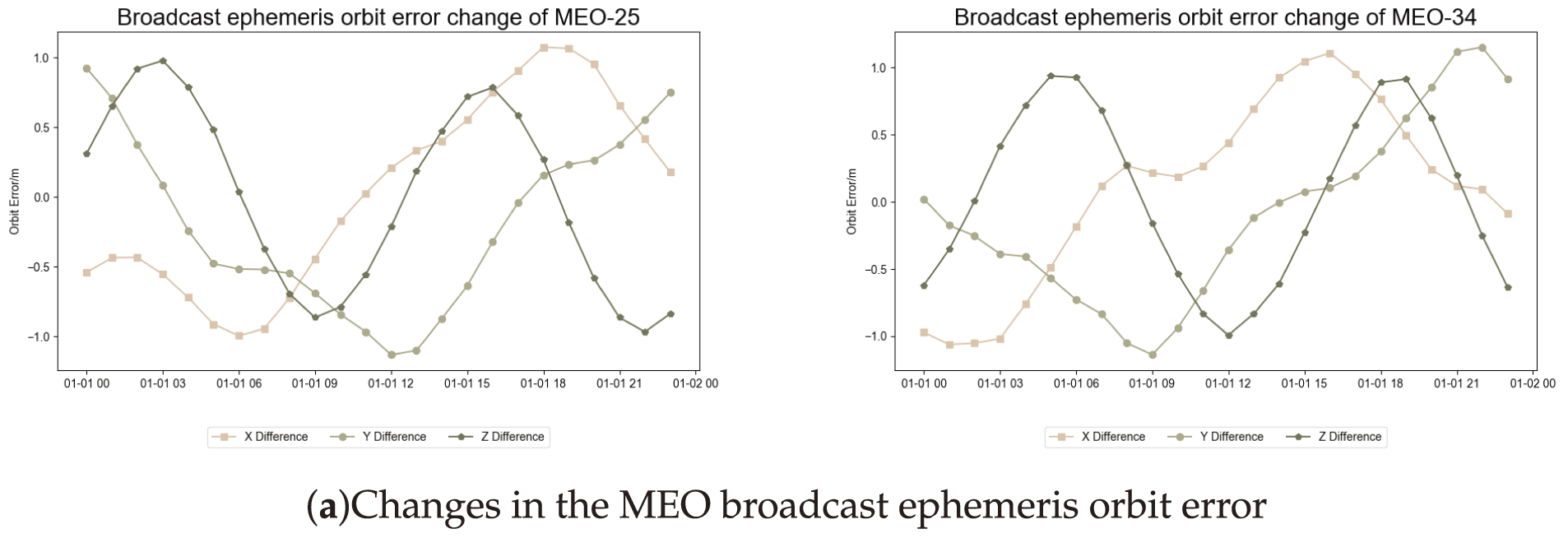
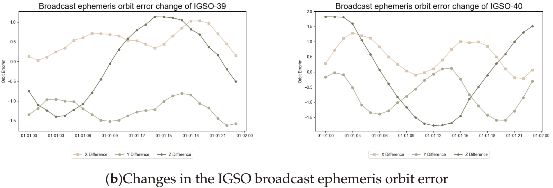
Figure 1: Trend in BDS-3 broadcast ephemeris error

2.2 Model Structure

A flowchart of the study is presented in Fig. 2. The inputs of the model were 6 broadcast ephemeris parameters and 9 perturbation correction parameters, with a total of 15 input features. These parameters contained key information about the satellite orbit and perturbation factors and can comprehensively describe the operational state of the satellite. In the first data processing step, the input features were sent to two parallel models for feature extraction: the AEBP and TR-BiLSTM models.

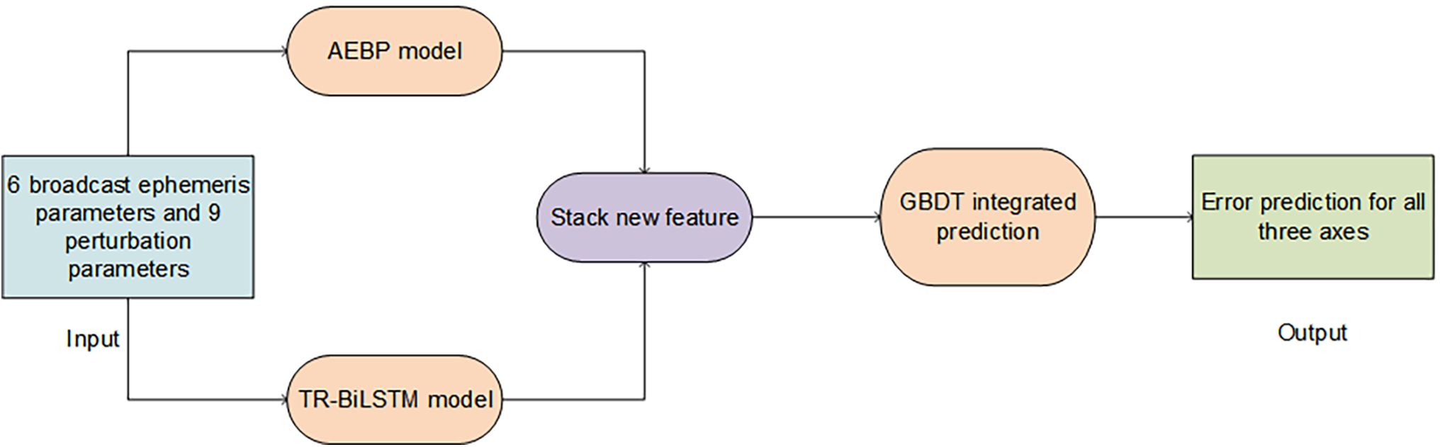
Figure 2: Model flow chart

After the AEBP and TR-BiLSTM models generated their respective feature sets, these features were sent to a feature stacking module. This module combined the outputs of the two models to create a new integrated feature set. By merging the distinct data processing capabilities of the AEBP and TR-BiLSTM models, the stacked features enhanced the expressive power and ability of the model to capture complex patterns in the data. Once feature stacking was complete, the new feature set was fed into a GBDT ensemble learning model for final error prediction. The GBDT model leveraged the strengths of multiple decision trees to improve forecasting performance. During the prediction process, each decision tree iteratively reduced the error of the previous prediction, thereby continuously refining the accuracy of the model. Specifically, the GBDT model was used to predict the error values for the three axes (X, Y, and Z) of the satellite orbit.

By integrating the AEBP model, TR-BiLSTM model, and GBDT model, this design fully exploited the advantages of the two neural networks and the powerful learning capabilities of GBDT. The AEBP model exceled in extracting static and local features, while the TR-BiLSTM model captured temporal patterns and global dependencies. The GBDT model further enhanced the prediction accuracy through its ensemble learning framework. Together, these components significantly improved the accuracy of the error prediction and the generalization ability of the overall model.

2.3 Attention-Enhanced BP Network Prediction Model

The proposed AEBP network prediction model integrated a feedforward neural network with a multihead self-attention mechanism to improve the accuracy of satellite orbit error predictions. In this model, the input layer received 15 features consisting of 6 broadcast ephemeris parameters and 9 perturbation parameters. Fig. 3 illustrates the overall structure of the AEBP model.

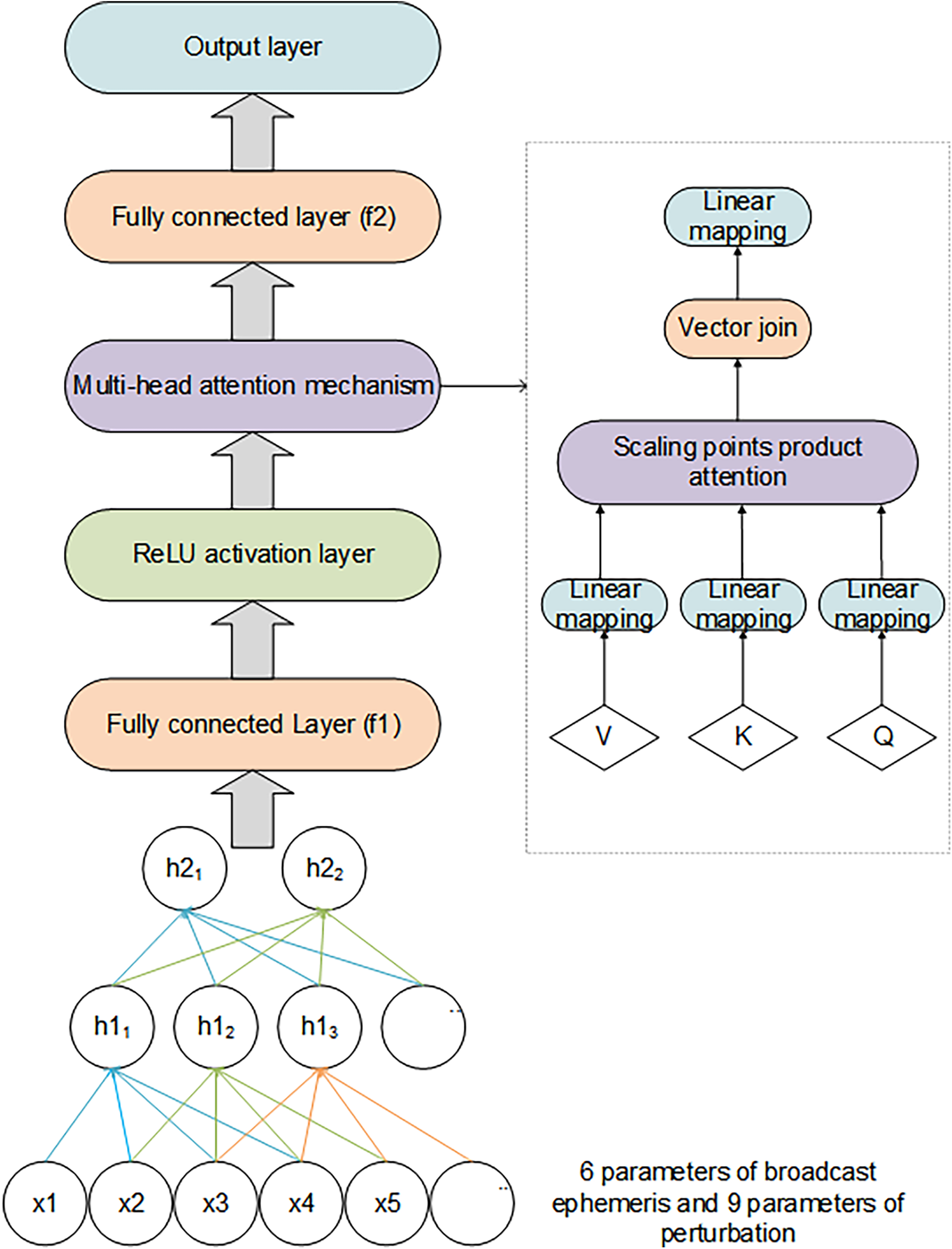
Figure 3: Structure diagram of the AEBP model

Initially, the raw input features x were fed into the first fully connected layer (fc1). This layer performed a linear transformation to map the 15-dimensional input onto a higher-dimensional latent space, thereby extracting the initial representation of the underlying features. This process is represented by

h1=fc1(x)(1)

The resulting hidden representation h1 was then passed through the ReLU activation function, which introduced nonlinearity into the model. This nonlinear transformation was crucial for allowing the network to capture complex relationships among the input parameters, as expressed by

h1′=ReLU(h1)(2)

Following a nonlinear transformation, the intermediate output h1′ was processed using the multihead self-attention mechanism. The primary goal of this mechanism was to allow the network to focus dynamically on the most informative parts of the input data. In practice, the mechanism first projects h1′ onto three separate spaces to form the query (Qi), key (Ki), and value (Vi) matrices. The attention mechanism computes the relevance of each input feature by calculating attention scores for each feature pair. The scores were computed as follows:

αi=softmax(QiKiTdk)Vi(3)

Here, dk denotes the dimensions of the key vectors. The softmax function normalized the computed scores, ensuring that they represented a proper probability distribution over the input features. This process enabled the model to assign higher weights to more relevant features, thereby producing an attention-modified output.

h2=∑iαiVi(4)

Output h2 encapsulated the dynamically weighted information of the input data and highlighted the most critical features of the prediction task.

Finally, the attention-weighted output h2 was passed through the second fully connected layer (fc2), which mapped the enhanced feature representation to the final prediction. This step was formulated as follows:

y=fc2(h2)(5)

Here, y denotes the predicted satellite orbit error. Therefore, the overall architecture combines the capacity of the traditional BP network for feature extraction with the dynamic feature selection capability of the multihead attention mechanism, enabling the model to handle noisy and redundant inputs effectively.

This integrated design is particularly beneficial in real-world applications, where input data are often corrupted by noise or contain irrelevant information. The multihead attention mechanism allows the network to assign varying levels of importance to different features, thereby enhancing the overall robustness and predictive performance of the model [17]. Fig. 3 provides a schematic illustration of the model structure, clearly depicting the flow of data from the input through fc1, ReLU activation function, multihead attention mechanism, and finally, fc2, thus producing the final prediction.

The AEBP model consists of an input layer with 15 neurons that correspond to the 15 input features (6 broadcast ephemeris parameters and 9 perturbation parameters). The first fully connected layer (fc1) maps the input to a hidden layer with 64 neurons, which is followed by a ReLU activation function. The multi-head attention mechanism, with its 8 attention heads, dynamically weights the hidden layer outputs by focusing on the most relevant features. The final fully connected layer (fc2) maps the attention-weighted outputs to 3 neurons, representing the predicted errors in the X, Y, and Z directions.

2.4 TR-BiLSTM Neural Network Model

In this study, a TR-BiLSTM-based neural network model was designed to capture the nonlinear characteristics of time-series data. This model combined three core structures–Transformer encoder, ResNet block, and BiLSTM layer–to leverage their advantages fully and aimed to capture the nonlinear characteristics of the time-series data and enhance the understanding of the temporal nature of the input series. This structure performed well in capturing the long-term dependency of a series and processing time-series data. The general structure of TR-BiLSTM is shown in Fig. 4.

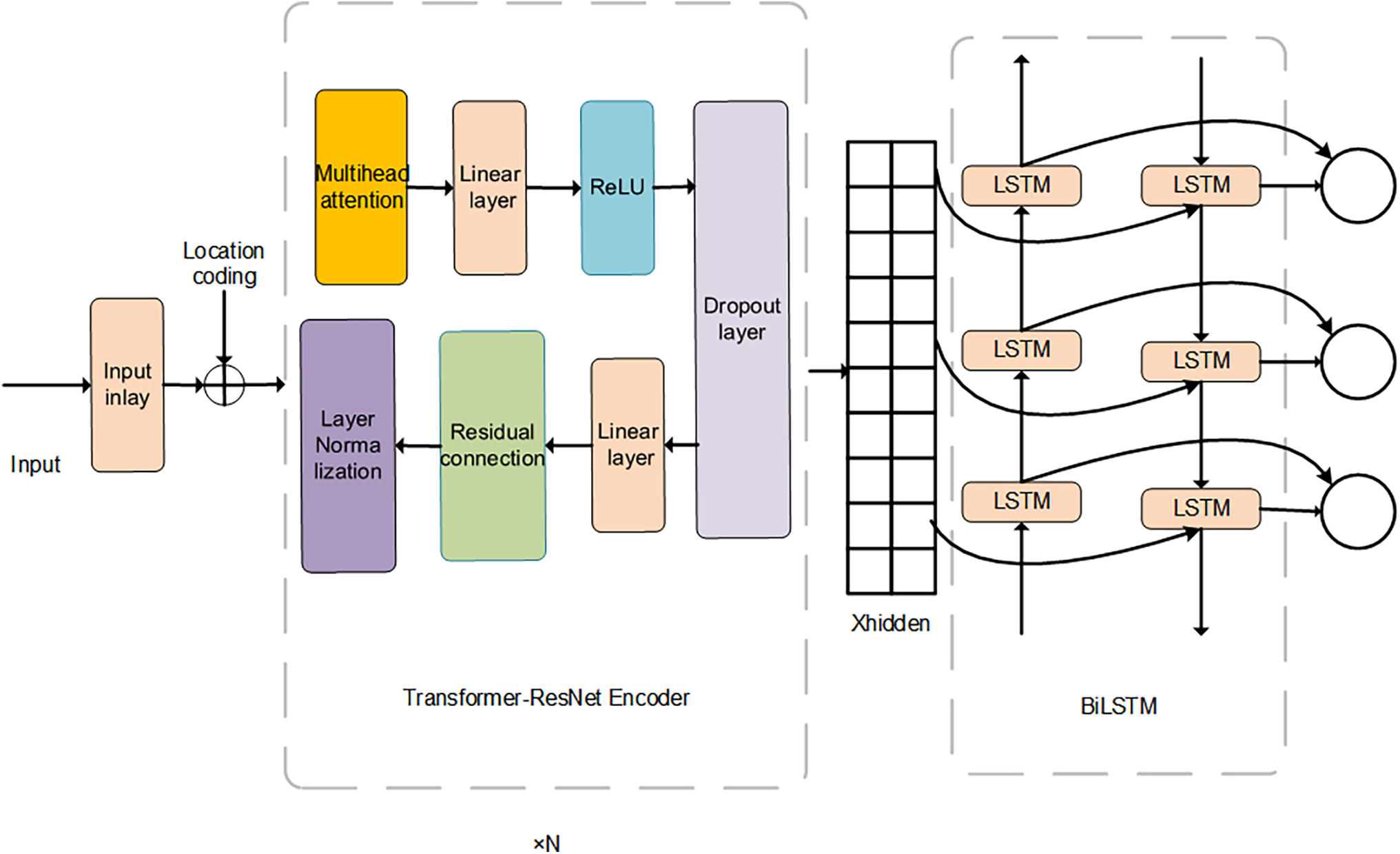
Figure 4: Structure diagram of TR-BiLSTM

The core of the Transformer [18] was the self-attention mechanism. Through its self-attention mechanism, the Transformer could process all the position information in the input sequence in parallel, providing the model with powerful feature extraction ability and rich information for subsequent processing steps. Because the Transformer did not contain position information, as in a recurrent neural network [19] or convolutional neural network [20], it used positional encoding to embed the position information of the elements in the sequence into a vector representation.

The core part of the model was a Transformer-ResNet-Encoder composed of multiple stacked Transformer-ResNet-Encoder layers. Each TransformerResNetEncoder layer contained two linear layers and residual connections, as well as layer normalization and a dropout layer [21]. By introducing a residual connection, the training difficulty of the deep network was alleviated, and the representation ability and training efficiency of the model were improved. In this manner, the Transformer encoder was capable of residual connection and layer normalization, thereby enhancing its feature extraction ability [22].

A residual network (ResNet) innovatively addresses the vanishing gradient problem in deep networks through the incorporation of skip connections. By allowing the network to learn the residuals between the inputs and outputs directly, ResNet not only facilitates the effective training of deeper architectures but also enhances their expressive power and predictive accuracy. This design is particularly innovative as it enables the model to capture essential features from input data more accurately, significantly improving both training efficiency and feature extraction capabilities. The integration of ResNet within the Transformer architecture represents a novel approach for enhancing deep learning performance by merging the strengths of both architectures.

The formulation for the residual connection in the Transformer layer is:

Output=LayerNorm(x+Attention(x))(6)

Here, x is the input to the layer and Attention(x) is the output from the self-attention mechanism. The term x+Attention(x) represents the skip connection, which allows the model to learn the residuals and makes it more efficient at capturing complex temporal patterns.

One of the key innovations in the TR-BiLSTM model is the bidirectional LSTM layer, which processes time-series data in both the forward and reverse directions. This bidirectional approach allowed the model to leverage both past and future contexts, thereby enhancing its ability to understand complex temporal dynamics, particularly satellite orbit prediction. By combining two independent LSTM layers that analyze the sequence chronologically and in reverse, BiLSTM captured long-term dependencies more effectively, resulting in richer representations of the input data. Finally, the output of the BiLSTM was mapped to the desired output space through a linear layer, providing a robust mechanism for accurate predictions.

The forward pass of an LSTM unit at time step t is calculated as follows:

h→t=LSTMforward(xt,h→t−1)(7)

Here, h→t represents the hidden state at time step t for the forward LSTM, and xt is the input at time step t.

The backward pass of the LSTM is:

h←t=LSTMbackward(xt,h←t+1)(8)

Here, h←t represents the hidden state for the backward LSTM at time step t.

The final BiLSTM output was the concatenation of the forward and backward hidden states.

ht=[h→t,h←t](9)

This bidirectional approach allowed the model to capture long-term dependencies in the input data, improving its ability to predict satellite orbits more accurately because it considered both past and future inputs.

Once the data had passed through the Transformer-ResNet Encoder and BiLSTM layer, the final feature representations were fed into the linear output layer to generate the final predictions:

y=fc2(hT)(10)

Here, y is the final predicted output and hT is the final hidden state from the BiLSTM layer, which contains the features learned from both the forward and backward passes.

The TR-BiLSTM model integrates a Transformer encoder with a bidirectional LSTM layer. The Transformer encoder captures global dependencies, whereas the BiLSTM layer captures long-term temporal patterns in the data. The number of neurons in the hidden layers is 64, which is consistent with the configuration of the AEBP model. This allows the model to handle complex time-series data while capturing both forward and backward temporal dependencies. The Transformer encoder processes the input data in parallel, whereas the BiLSTM processes the data in a sequential manner, ensuring that both local and global features are effectively learned.

2.5 Ensemble Learning Prediction Model

2.5.1 Model Structure

GBDT, i.e., gradient boosting tree [23], is an ensemble algorithm based on decision trees. Gradient boosting is an ensemble boosting algorithm that iterates on a new learner through a gradient descent. Gradient boosting involves a decision tree-based ensemble technique that sequentially trains weak learners to improve the overall performance of the model, with the goal of combining multiple weak predictors into a strong predictive model. In each generation, it calculates the negative gradient of the loss function, that is, the residuals, fits a new weak model to predict the residuals [24], and adds it to the model. The predicted values for each model are added to obtain the final model-predicted values. The main advantage of the gradient boosting algorithm is that it can continuously fine-tune the model performance by studying the mistakes made by prior models, thereby gradually enhancing model accuracy. Fig. 5 shows a schematic of the GBDT model.

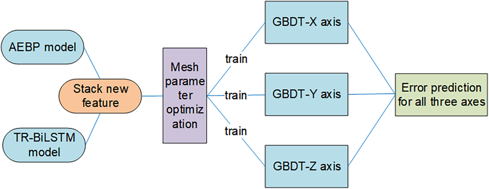
Figure 5: Structural diagram of the GBDT model

GBDT is an ensemble learning algorithm based on decision trees. Each tree was sequentially trained to correct the residuals (errors) of the previous tree. The iterative process for training the model is as follows.

Update the Formula: In iteration, the model was updated by adding a new weak learner hm(x) (decision tree) that predicted the residuals (negative gradients) of the previous model.

fm(x)=fm−1(x)+η⋅hm(x)(11)

Here, fm(x) denotes the prediction of the model after m trees. η denote the learning rate that controls the contribution of each new tree to the final model prediction. hm(x) is the mth weak learner (decision tree) that fits the residuals.

Final Prediction: The final prediction is the predictions of the sum of all trees weighted by the learning rate:

f(x)=∑m=1Mη⋅hm(x)(12)

Here, f(x) is the final prediction, M the number of trees in the model, and hm(x) the prediction from the mth decision tree.

The innovation of this model lies in integrating GBDT with attention-based and temporal feature extraction models, specifically AEBP and TR-BiLSTM. This integration improves the prediction accuracy and model stability by allowing GBDT to iteratively correct errors based on the outputs of more advanced neural network models that focus on the most relevant features (via attention mechanisms) and capture long-term dependencies (via BiLSTM). This fusion leverages the strengths of both residual learning in GBDT and feature extraction in AEBP and TR-BiLSTM, leading to a superior performance in satellite orbit prediction tasks.

The interaction between AEBP and TR-BiLSTM occurs at the feature stacking stage. Specifically, the AEBP model and the TR-BiLSTM model independently predict the satellite orbit error and output the prediction error in each direction (X, Y, Z axis). The AEBP model outputs local static error information about the track, while the TR-BiLSTM model outputs dynamic timing error information about the track. The output of these models is the prediction error, which is then combined by stacking operations to form a new 6-dimensional feature vector. The interaction of each model in the stacking process is reflected in two ways:

Information fusion: The output of the AEBP model and the output of the TR-BiLSTM model are merged as a feature vector. This fusion combines the static and dynamic information to provide a more comprehensive error prediction input.

Model prediction is enhanced: With stacked 6-dimensional features, the GBDT model can make further error predictions based on these two different types of error information, and it can continuously optimize the prediction results. GBDT adjusts the weights in each round of iterations to reduce the residual error of previous predictions, so as to gradually improve the overall prediction accuracy.

2.5.2 Model Process

Step 1: Identify the input and output of the model and establish the neuron count in each layer.

In addition to the epoch time and the six Kepler orbital radical parameters, this study adds 9 perturbation correction term parameters: the network model receives 15 input parameters, errors of the X, Y, Z axes of the satellite are the outputs, the output layer contains 15 neurons, there are 3 neurons, and the neuron count of the hidden layer is determined by an empirical formula:

r=a+b+c,c∈[1,10](13)

Missing values were handled on the data, and the mean value was used to fill the missing values to ensure there were no missing values. Different feature magnitudes may lead to problems during gradient updating or slower convergence. To prevent the various magnitudes of each parameter from affecting the network training, each parameter was normalized before training so that it was mapped to the range of [−1, 1], which ensured stable gradient descent performance. The stability and convergence speed of the model were improved by seeking an optimal solution, and the learning rate problem caused by large or small eigenvalues was avoided.

Step 2: Define the two models and predict their errors.

The AEBP and TR-BiLSTM models are defined, the multihead attention mechanism is added to the feedforward neural network model, 15 parameters are added to the Transformer, BiLSTM is connected to the vector of the hidden layer, and the loss function and optimizer are defined. The output results are obtained using the BiLSTM layer. Training was performed separately and error was predicted.

Step 3: Use the outputs of the two models as inputs for ensemble learning during training.

The outputs of the AEBP and TR-BiLSTM models are used as inputs for ensemble learning, and the prediction results are stacked to form a new feature. The AEBP and TR-BiLSTM models are used as primary learners, and the gradient boosting regressor GBDT is used for the construction and training of the metamodel. This metamodel uses three independent gradient-boosted regressors to predict the values of the three axes.

Grid search parameters [25] were defined for tuning to determine the optimal combination of parameters. The evaluation indicator was neg_mean_squared_error. Using 10-fold cross-validation [26], the optimal parameters were obtained. Different combinations of parameters, such as n_estimators (number of estimators), learning_rate (learning rate), and max_depth (maximum depth), were used as tuning parameters. Next, three gradient boosting regressor models were instantiated: boosted_model_X, boosted_model_Y, and boosted_model_Z. New features and objects were used for training, and three models were used for prediction along the X-, Y- and Z-axes to obtain the prediction results in the three directions. The modeling process is shown in Fig. 6.

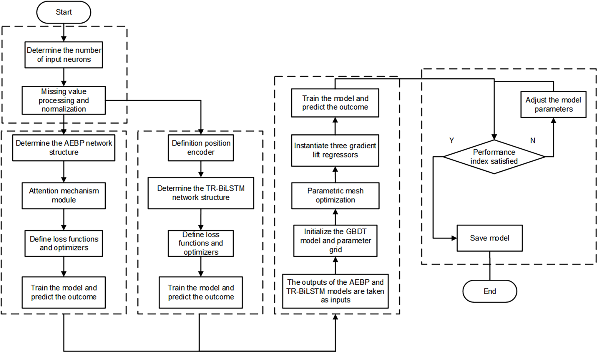
Figure 6: Structural diagram of the ensemble learning process

Step 4: Save the model

If the prediction result satisfies the performance index, then the model is saved. If the prediction results do not meet the requirements, the model parameters are continuously adjusted, the parameter range is expanded, and the grid search parameters are optimized until the performance index is met. Subsequently, the model is saved to complete the process.

The orbital height of MEO satellites is usually high, is affected by the gravity of the sun and the moon, and has perturbations that change slowly; thus, small adjustments are usually needed. The main sources of perturbation are the non-spherical gravitational field of the Earth, the gravity of the sun and the moon, and the solar radiation pressure. The orbital perturbation of the IGSO satellite shows different characteristics because its orbit is inclined, which results in periodic changes in its orbital period. In particular, the non-spherical gravitational field of the Earth, the gravity of the sun and the moon, and the periodic perturbations caused by orbital tilt may have a considerable influence on the position and orbital stability of the satellite. Although MEO satellites typically experience smooth perturbations and relatively few of them, IGSO satellites may experience significant and complex perturbations due to their orbital tilt. The following is the weight distribution process for the three models.

Both the AEBP and TR-BiLSTM models automatically adjust their weights through backpropagation and gradient descent to minimize prediction errors. The AEBP model uses uniform distribution to initialize the weights at the start of training. After the input features are propagated forward, they are multiplied with the weight matrix and the output is generated by the ReLU activation function. Finally, the prediction error is calculated. Then, the model uses the mean square error loss function to guide the backpropagation, calculates the weight gradient, and adjusts the weights through the Adam optimizer so that the model can continuously optimize the feature weights and improve the prediction accuracy. The TR-BiLSTM model maps the input to a hidden space through the embedding layer, and it learns the relationship between the input features and the weights using the self-attention mechanism. During training, the model calculates the error between the predicted value and the actual value and adjusts its weights through backpropagation and gradient descent to minimize the loss function. The adjustment of weights is completely dependent on the training data, and the model automatically learns the importance of each input feature and dynamically optimizes the corresponding weights.

The GBDT model determines the weight by calculating the contribution of each feature to error reduction when the decision tree is split. At each round of training, the model selects features to split based on error optimization. The more frequently the features appear at the split point of the tree, the greater their contribution to error reduction and the higher their weight. GBDT continuously optimizes the feature weights by reducing residuals, so that the model can effectively evaluate the influence of each input feature on the prediction results. Compared with the AEBP and TR-BiLSTM deep learning methods, GBDT uses decision trees to improve prediction performance. The adjustment of feature weights depends on the contribution of the data features in the tree structure, which can automatically learn the importance of features and optimize prediction accuracy.

The orbital characteristics of different satellites affect the weight distribution of input features in each model. The perturbation change in the orbit of the MEO satellite is relatively stable, so the weight adjustment of the model is small. IGSO satellites, on the other hand, are more affected by perturbations due to their orbital tilt, so their weight will change significantly with the change in their orbit. Different satellite orbits have different effects on the learning process of the model, and the model learns the relationship between input features and output results by automatically adjusting its weights. This data-driven, automatic learning mechanism ensures that each model can adapt to the characteristics of different tracks, thereby improving the accuracy and stability of the predictions.

2.5.3 Computational Complexity

Because of the complexity and multiplicity of the model, this study analyzed its computational complexity by integrating two advanced predictive models, one that combines an attention-enhanced BPNN with another that integrates the Transformer, ResNet, and BiLSTM, using a GBDT framework. Although each base model has high computational complexity (for instance, the attention mechanism has a complexity of O(n2⋅d), and TR-BiLSTM involves sequential operations); the overall computational burden was primarily determined by the GBDT fusion process. Building an ensemble with GBDT required constructing M decision trees overN samples, resulting in a time complexity of O(M⋅N⋅log⁡(N)) and a space complexity of O(M⋅K), where K is the maximum depth of the trees.

This integration effectively leveraged the strengths of both base models while mitigating their weaknesses. Offline optimization techniques, such as grid and random searches, were used to fine-tune hyperparameters and manage the overall computational cost. Despite the high complexity of the individual components, the carefully optimized ensemble delivered real-time predictions with improved accuracy and robustness, making it practical for real-world satellite navigation applications.

2.5.4 Operating Environment and Parameter Settings

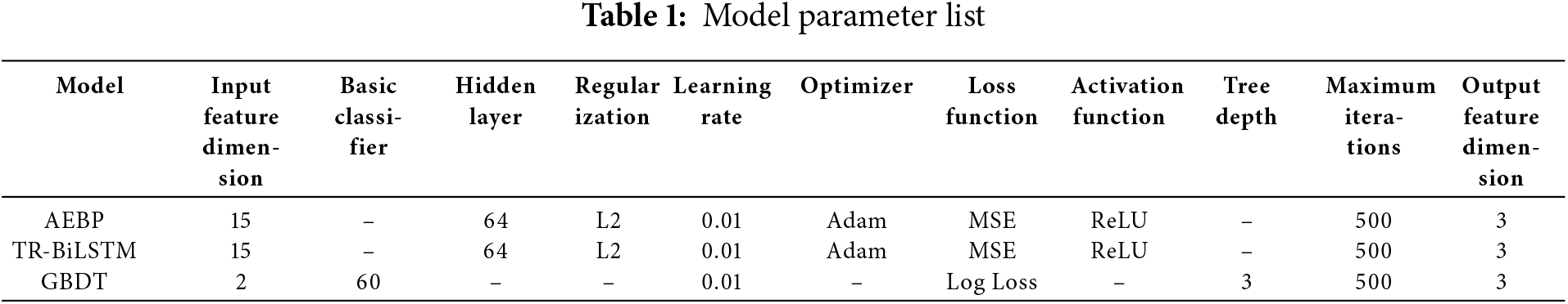
This experiment covered two types of data collected from four satellites from August 12 to 16, 2024. This included two types of satellite. The samples were subdivided, and features were extracted to form 1038 16-dimensional samples. All experiments were performed in a PyCharm environment. The computer system used was the Win10 (64-bit) operating system, with 8 GB of RAM, a Core i5-10200H processor (2.4 GHz, quad-core, eight threads), and a GeForce GTX 1650 graphics card. Table 1 lists the parameters of the AEBP, TR-BiLSTM, and GBDT methods.

3  Model Validation and Result Analysis

3.1 Model Validation

In this study, BDS satellites with PRNs 25 and 34 were selected to represent MEO satellites, and BDS satellites with PRNs 39 and 40 were chosen to represent IGSO satellite orbit types for model validation. The sampling frequency of the BDS broadcast ephemeris data was 1 h, and that of the precision ephemeris data was 5 min. Therefore, the precision ephemeris data were sampled every hour to unify the times between the two. In the same epoch, the orbit error was obtained from the difference between the satellite position calculated by the BDS broadcast ephemeris and the satellite position information extracted by the precision ephemeris at the corresponding time. Fifteen parameters were subsequently used as inputs for the AEBP, TR-BiLSTM, and GBDT models. Data from 12 to 15 August 2024, were used to train the models, and data from 16 August 2024, were used to test the models for forecasting errors. The model outputs were the errors in the XYZ directions Δx, Δy, and Δz. Each model was evaluated and corrected, and the output results of the revised models were compared.

This study examined the root mean square (RMS) error, standard deviation (STD), and mean (mean) to evaluate the accuracy and consistency of the model prediction results. RMS errors quantify the deviation between the predicted values and actual observations, making it one of the most frequently employed evaluation measures. A lower value indicates that the predictions of the model align more closely with the exact values. STD represents the degree to which the predicted value deviates from the actual value, reflecting the degree of dispersion of the values in the dataset. The smaller the STD, the more stable the predicted value. Mean reflects the average deviation between the predicted and actual observed values of the model. The closer the mean is to zero, the more accurately the model predicts the overall trend.

To validate the capability of the model to predict the orbital data of BDS satellites, the perturbation-corrected parametric neural network AEBP model, TR-BiLSTM model, and GBDT ensemble learning models were employed for orbit prediction. For comparative experiments, the BPNN, LSTM, PSO-BP, and IPSO-BP models were included. Seven models and their experimental data were compared for the MEO and IGSO satellites of BDS-3.

In the comparative analysis, BPNN and LSTM, as traditional neural network models, effectively addressed the nonlinear relationships present in the data. The PSO-BP [9] and IPSO-BP [10] models incorporated optimization strategies that enhance training efficiency and improve overall model performance. Utilizing a diverse range of algorithms ensured a comprehensive assessment of orbit prediction capabilities, reinforcing the reliability of the results with performance metrics such as RMSE and MAE. This varied selection of models leads to more robust conclusions and ensures accurate predictions of MEO and IGSO satellite orbital data of BDS-3.

3.2 MEO Satellite Orbit Prediction Results

In the experiments, C34 was chosen to represent the MEO satellite orbit type, and the specific orbit error prediction results of the BDS-3 MEO satellite C34 are depicted in Fig. 7.

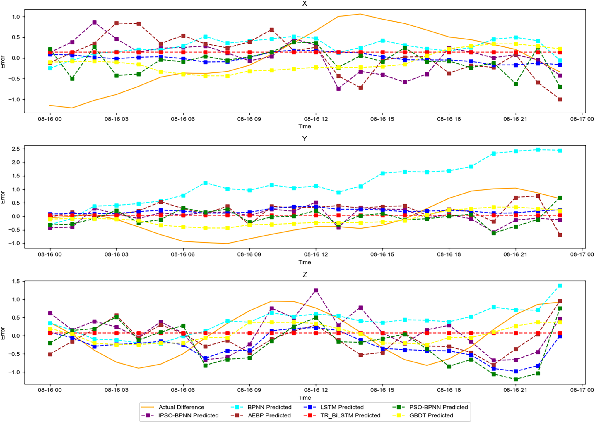
Figure 7: Diagram of orbit error prediction for the MEO-C34 satellite

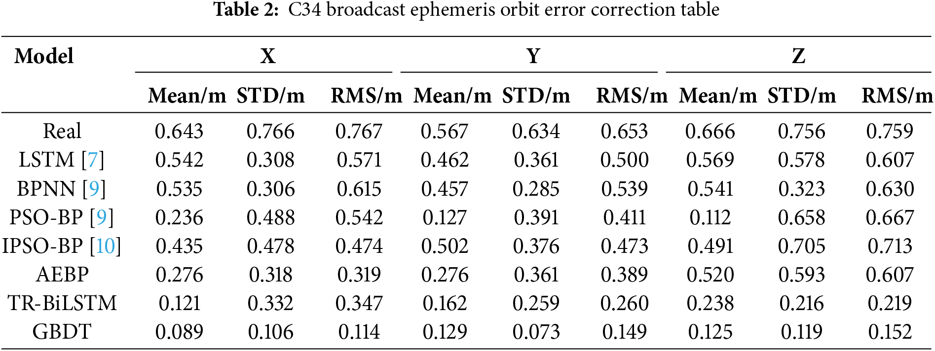
For the C34 satellite, the evaluation indicators of the broadcast ephemeris orbit error for each model are presented in Table 2. The values of the indicators of the BPNN and LSTM models were lower than the actual values of the three evaluation indicators, indicating that the BPNN and LSTM models could effectively predict and reduce satellite orbit errors. The mean value and RMS of the AEBP model were both lower than those of the BPNN and LSTM models. In contrast, the standard deviation of the AEBP model was close to the values of the BPNN and LSTM models, indicating that the AEBP model had a higher accuracy in predicting satellite orbit errors. Compared to the first three models, the TR-BiLSTM model showed a modest increase in prediction accuracy, but its stability was not high. Compared with the other four models, the GBDT model not only improved the accuracy but also the stability of the model prediction; both the accuracy and stability of the prediction error significantly improved. The orbit error predicted through ensemble learning can be effectively reduced and kept within the range of –0.3 to 0.4 m. Compared with those of the AEBP and TR-BiLSTM neural networks, the error correction rates of satellite orbits in the three directions increased by 30.9%∼50.6% and had better stability.

3.3 IGSO Satellite Orbit Prediction Results

In the experiments, the BDS of C40 among the BDS-3 IGSO satellites was selected to represent the orbit type of IGSO satellites. The specific orbit error prediction results are shown in Fig. 8.

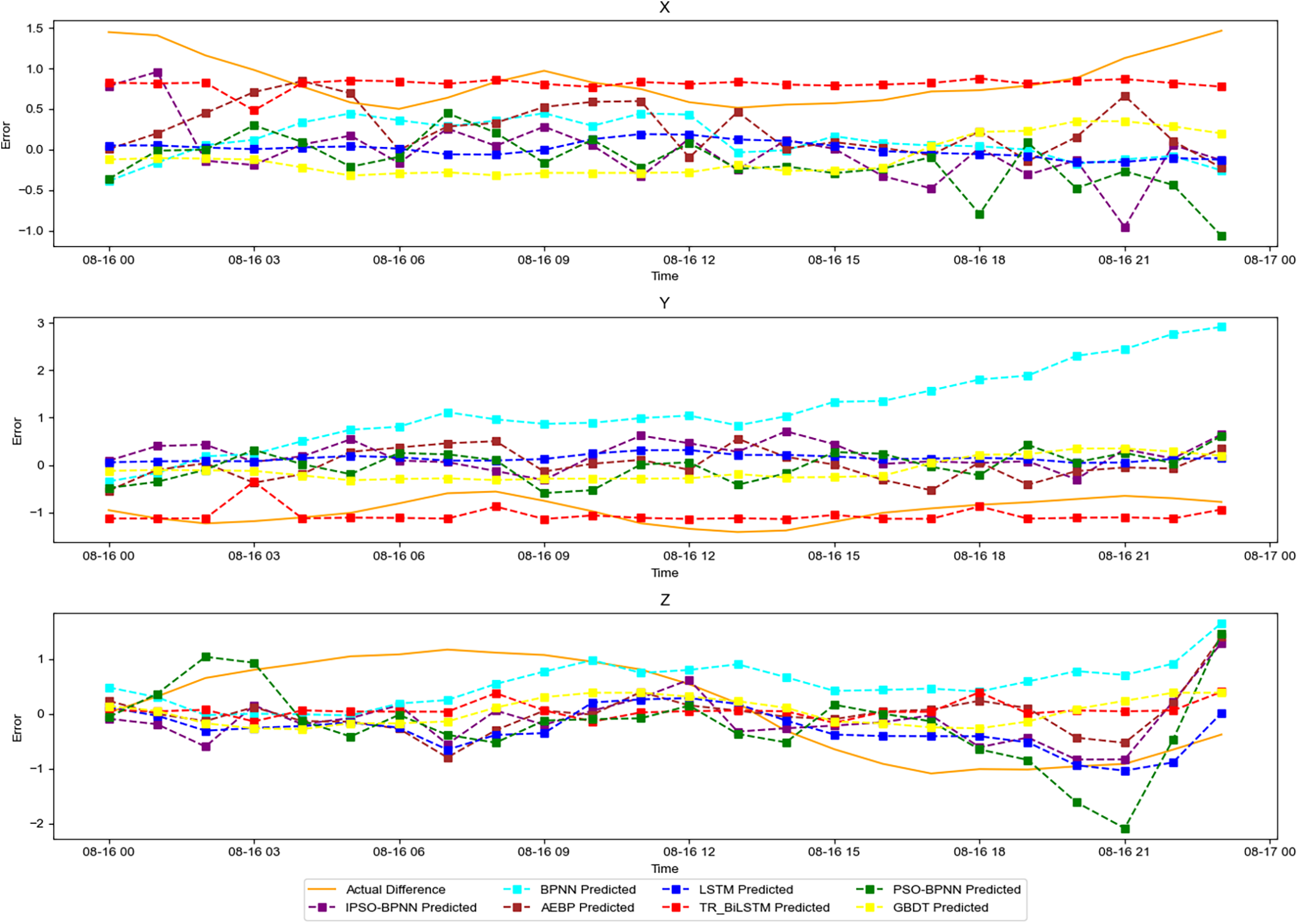
Figure 8: Diagram of orbit error prediction for the IGSO-C40 satellite

For the C40 satellite, the evaluation indicators of the broadcast ephemeris orbit error for each model are compared in Table 3. Compared with those of the traditional BPNN and LSTM models, the mean value of the AEBP model is greater than the mean values of the BPNN and LSTM models, indicating that the overall trend predicted by the AEBP model has no effect. The BPNN and LSTM models were accurate; the RMS of the AEBP model was smaller than those of the BPNN and LSTM models in only one direction, indicating that the prediction outcomes of the BPNN and LSTM models were more aligned with the actual values. The STD of the AEBP model was in two directions and was lower than those of the BPNN and LSTM models, indicating that the prediction results of the AEBP model were relatively stable. Fig. 8 shows that the prediction errors of the AEBP model. The true values closely overlap, indicating that the model can fit the data well but cannot correct the orbit error satisfactorily.

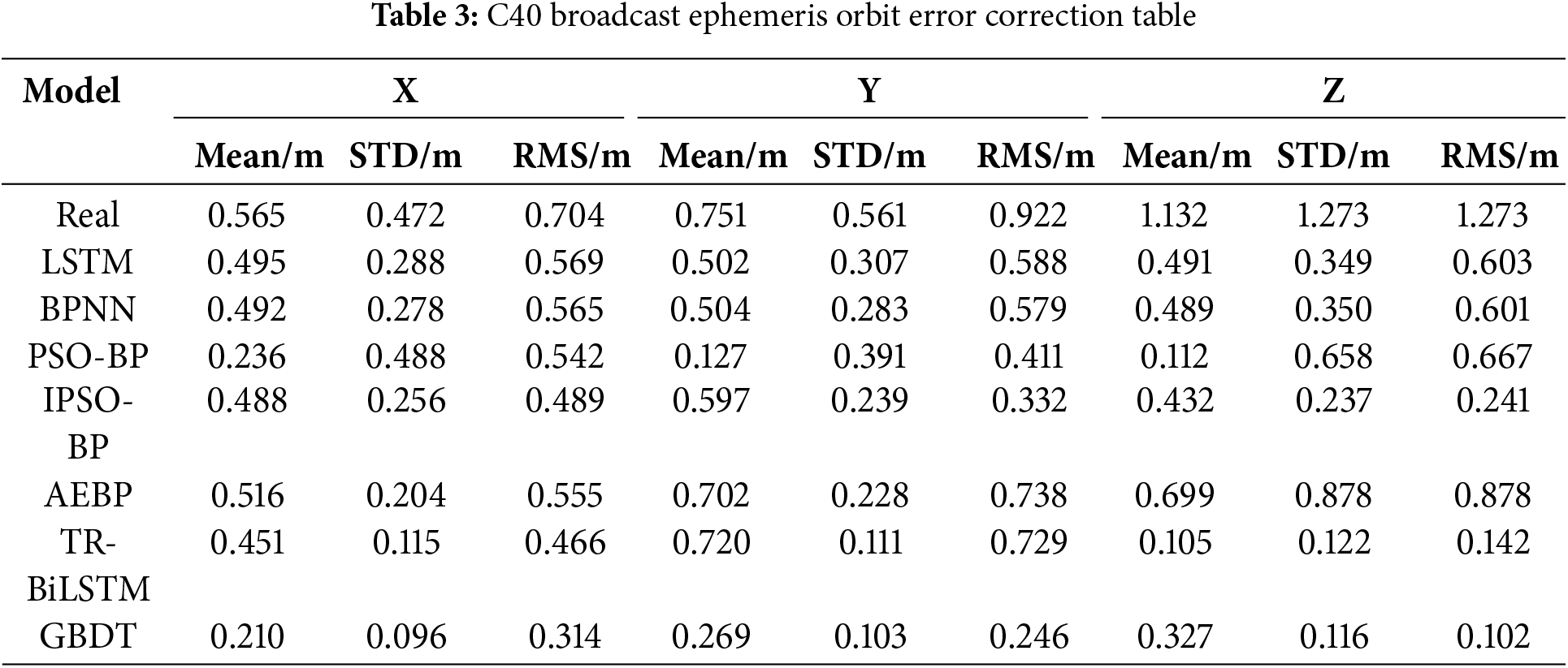
The TR-BiLSTM model exhibited lower RMS and STD values than the BPNN, LSTM, and AEBP models. Only one direction of the mean value was more significant than those of the other models, indicating that the overall trend and results predicted by the TR-BiLSTM model were close to the actual values. The TR-BiLSTM model was prone to changes, the predicted value was insufficiently stable, and the error curve was not sufficiently smooth.

The RMS and STD of the GBDT model were lower than those of the BPNN, LSTM, AEBP, PSO-BP, IPSO-BP, and TR-BiLSTM models; however, the overall prediction trend was relatively stable. Fig. 8 shows that the prediction error of the GBDT model was stable at approximately −1∼1 m, and the prediction accuracy and stability of this model were greater than those of the other four models.

3.4 Analysis

To improve the applicability of the results, the C25 satellite in the MEO orbit and the C39 satellite in the IGSO orbit were included in the experimental data. The performances of various machine learning models in satellite navigation systems were evaluated in detail. First, a BPNN model was used. This model had an average performance for most satellites; however, it exhibited a better performance for a small number of satellites. Second, the extended LSTM was used. This model showed good fitting ability for satellite data that needed to consider time-series information, but its performance under some satellites was slightly mediocre. The AEBP model yielded good fitting results for simple datasets; however, its performance for complex datasets was mediocre. Notably, although the performance of the TR-BiLSTM model was not stable for different satellites, it demonstrated better performance in processing sequence data, especially when addressing long-term dependencies. Finally, the GBDT algorithm was used, which enhanced the overall performance of the model by combining multiple weak classifiers and demonstrated strong results in both the correction rate and mean square error.

Table 4 shows the comparison table of the error correction rates of the MEO and IGSO satellites. Compared to those of the traditional BPNN and LSTM models, the error correction rate of the AEBP model increased by 12.8%∼23.6%. Fig. 9 shows that the prediction errors of the AEBP model and the true values closely overlap, indicating that the model can fit the data well but cannot correct the orbit error satisfactorily. The AEBP model has certain limitations in addressing this nonlinear and complex trend.

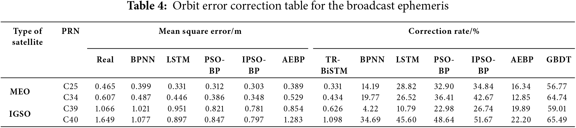
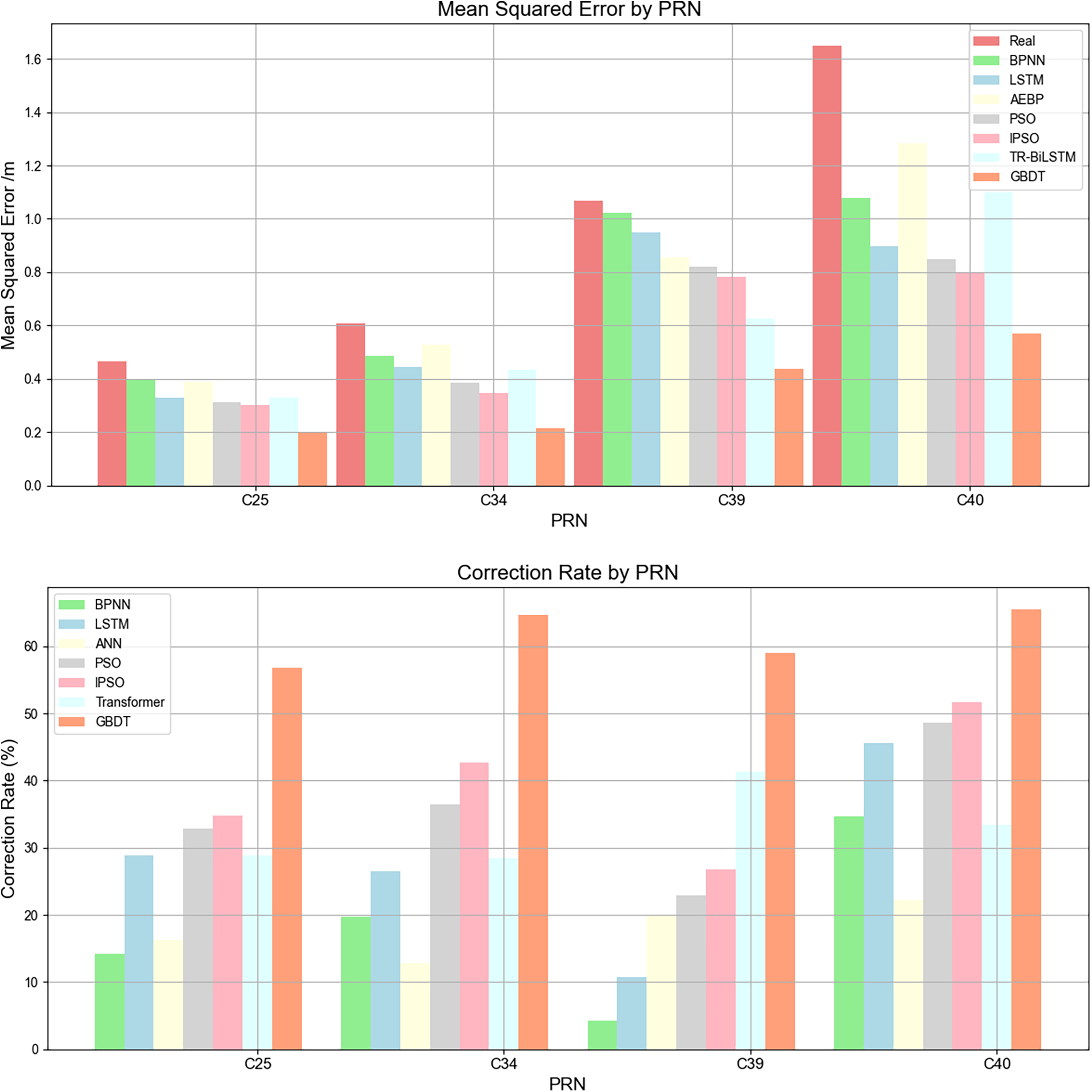
Figure 9: Comparison of the model mean square error and modification rate

The errors of the TR-BiLSTM forecast model were all below the true values, but the instability could not be eliminated. The TR-BiLSTM model achieved a higher forecast accuracy than the AEBP model; however, there were still specific errors and instabilities. Compared with those of the AEBP model, the prediction error correction rates of the TR-BiLSTM model increased by 14.9%∼26.6%, and the actual error correction rates increased by 28.5%∼41.2%.

Compared with the first two models, the GBDT ensemble learning model exhibited the lowest correction error, showed less fluctuation, was more stable and reliable, and could correct real errors well. By combining multiple forecast models, GBDT ensemble learning can improve the overall forecast accuracy and stability. This method fully utilizes the advantages of each model and effectively reduces the prediction error of a single model. Compared with those of the TR-BiLSTM model, the prediction error correction rates of the GBDT ensemble model increased by 30.9%∼50.6%, and the true error correction rates increased by 56.7%∼65.4%.

In this study, the performances of different machine learning models in satellite navigation systems were analyzed using box plots. Fig. 10 illustrates the performance of each model based on the MSE and modification rate. The figure shows the significant differences between the different models. The GBDT model exhibits the lowest median mean square error (approximately 0.3 m), indicating its excellent performance in terms of prediction accuracy. In contrast, the median mean square error of the AEBP model was approximately 0.5 m, which was the highest among the models, indicating that its predictive performance was relatively weak. Additionally, the performances of the LSTM model and BPNN model were relatively stable, with median mean square errors of approximately 0.45 and 0.5 m, respectively, indicating their general performance in forecasting. The median mean square error of the TR-BiLSTM model was approximately 0.4 m, indicating good and stable performance.

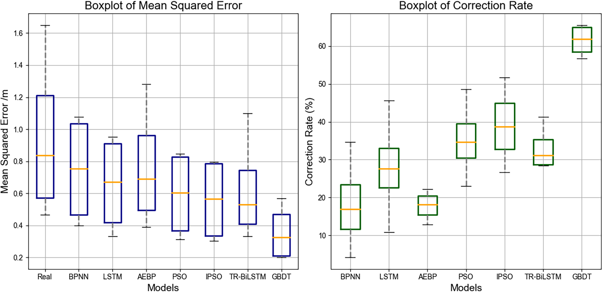
Figure 10: Box plot of the model mean square error and comparison of modification rate

Additionally, the figure shows the performance of each model in terms of correction rate. The GBDT model performed well in terms of revision rate; it presented high revision rates in most cases, indicating its excellent performance in correction prediction. The TR-BiLSTM model also exhibited a higher revision rate in most cases, indicating its excellent performance in correcting the prediction bias. In contrast, the revision rate of the BPNN model was low in some cases, indicating its insufficiency in correcting the predictions. The performance of the LSTM and AEBP models in terms of the correction rate was relatively average, and further improvement was required to increase their correction ability.

4  Conclusions

This study proposes an ensemble learning approach that utilizes GBDT to integrate predictions of the AEBP model and TR-BiLSTM model for BDS satellite orbit prediction.

The GBDT framework plays a crucial role in enabling the effective combination of the AEBP and TR-BiLSTM models. This novel integration allows the ensemble to leverage the strengths of both models while addressing their limitations. The GBDT method further optimizes the overall performance by assigning weights to and combining the outputs of the two models.

The AEBP model features a key innovation in its integration of an attention mechanism with BPNN, enhancing its ability to learn complex relationships among input features. This combination improves the ability of the model to focus on relevant information, significantly boosting prediction accuracy.

The TR-BiLSTM model demonstrates its innovation by integrating three key modules: the Transformer, which excels at capturing long-range dependencies; ResNet, which improves the gradient flow and accelerates convergence; and BiLSTM, which processes input sequences bidirectionally to capture comprehensive temporal patterns. This synergy effectively enhances the capability of the model to handle intricate time-series data.

The effectiveness of the proposed ensemble learning model is validated using the BDS broadcast ephemeris data for the BDS-3 MEO and IGSO satellites, showing that the model can correct broadcast ephemeris orbit errors with an error correction rate of up to 65.4%. This demonstrates the potential of the proposed method to improve the positioning accuracy of satellite navigation systems.

Acknowledgement: The authors sincerely appreciate the editors and reviewers for their valuable time and insightful feedback, which have greatly contributed to improving this work. We would like to thank Editage for English language editing.

Funding Statement: This research was funded by the Strategic Priority Research Program of the Chinese Academy of Sciences (Grant No. XDA28040300), Project for Guangxi Science and Technology Base, and Talents (Grant No. GK AD22035957), the Informatization Plan of the Chinese Academy of Sciences (Grant No. CAS-WX2021SF-0304), and the West Light Foundation of the Chinese Academy of Sciences (Grant No. XAB2021YN19).

Author Contributions: Conceptualization, Ruibo Wei and Mengzhao Li; methodology, Ruibo Wei and Mengzhao Li; software, Ruibo Wei; validation, Feng Liu and Yao Kong; formal analysis, Ruibo Wei and Mengzhao Li; investigation, Feng Liu and Fang Cheng; resources, Ruibo Wei and Mengzhao Li; data curation, Ruibo Wei and Mengzhao Li; writing—original draft preparation, Ruibo Wei and Mengzhao Li; writing—review and editing, Ruibo Wei and Mengzhao Li; visualization, Ruibo Wei and Mengzhao Li; supervision, Feng Liu and Fang Cheng; project administration, Feng Liu and Fang Cheng; funding acquisition, Feng Liu. All authors reviewed the results and approved the final version of the manuscript.

Availability of Data and Materials: The data that support the findings of this study are openly available in the International GNSS Service (IGS) at https://igs.org/products (accessed on 14 April 2025).

Ethics Approval: Not applicable.

Conflicts of Interest: The authors declare no conflicts of interest to report regarding the present study.

References

1. Zhang Y, Li Z, Li R, Wang Z, Yuan H, Song J. Orbital design of LEO navigation constellations and assessment of their augmentation to BDS. Adv Space Res. 2020;66(8):1911–23. doi:10.1016/j.asr.2020.07.021. [Google Scholar] [CrossRef]

2. Zhao Q, Guo J, Wang C, Lyu Y, Xu X, Yang C, et al. Precise orbit determination for BDS satellites. Satellite Navig. 2022;3(1):2. doi:10.1186/s43020-021-00062-y. [Google Scholar] [CrossRef]

3. Srivastava VK, Mishra P. Sun outage prediction modeling for Earth orbiting satellites. Aerosp Syst. 2022;5(4):545–52. doi:10.1007/s42401-022-00149-7. [Google Scholar] [CrossRef]

4. Liang T, Nie K, Li Q, Zhang J. Advanced analytical model for orbital aerodynamic prediction in LEO. Adv Space Res. 2023;71(1):507–24. doi:10.1016/j.asr.2022.09.005. [Google Scholar] [CrossRef]

5. Zhang J, Liu Y, Tu Z. Exploring fundamental laws of classical mechanics via predicting the orbits of planets based on neural networks. Chin Phys B. 2022;31(9):094502. doi:10.1088/1674-1056/ac8d88. [Google Scholar] [CrossRef]

6. Yang R, Song Z, Chen L, Gu Y, Xi X. Assisted cold start method for GPS receiver with artificial neural network-based satellite orbit prediction. Meas Sci Technol. 2020;32(1):015101. doi:10.1088/1361-6501/abac25. [Google Scholar] [CrossRef]

7. Kim B, Kim J. Prediction of IGS RTS orbit correction using LSTM network at the time of IOD change. Sensors. 2022;22(23):9421. doi:10.3390/s22239421. [Google Scholar] [PubMed] [CrossRef]

8. Mahmud MS, Zhou Z, Xu B. LSTM-driven prediction of orbital parameters for accurate LEOopportunistic navigation. In: ION GNSS+, The International Technical Meeting of the Satellite Divisionof The Institute of Navigation; 2024 Sep 16–20; Baltimore, MD, USA. p. 3542–55. doi:10.33012/2024.19869. [Google Scholar] [CrossRef]

9. Chen H, Niu F, Su X, Geng T, Liu Z, Li Q. Initial results of modeling and improvement of BDS-2/GPS broadcast ephemeris satellite orbit based on BP and PSO-BP neural networks. Remote Sens. 2021;13(23):4801. doi:10.3390/rs13234801. [Google Scholar] [CrossRef]

10. Peng J, Liu F, Hu W. BDS-3 broadcast ephemeris orbit correction model based on improved PSO combined with BP neural network. Comput Intell Neurosci. 2022;2022(1):4027667–12. doi:10.1155/2022/4027667. [Google Scholar] [PubMed] [CrossRef]

11. Jiao G, Song S, Liu Y, Su K, Cheng N, Wang S. Analysis and assessment of BDS-2 and BDS-3 broadcast ephemeris: accuracy, the datum of broadcast clocks and its impact on single point positioning. Remote Sens. 2020;12(13):2081. doi:10.3390/rs12132081. [Google Scholar] [CrossRef]

12. Jiang N, Cao Y, Xia F, Huang H, Meng Y, Zhou S, et al. Broadcast ephemeris SISRE assessment and systematic error characteristic analysis for BDS and GPS satellite systems. Adv Space Res. 2024;73(10):5284–98. doi:10.1016/j.asr.2024.02.021. [Google Scholar] [CrossRef]

13. Jian HJ, Wang Y, Zhang S. Accuracy evaluation of broadcast ephemeris for BDS-2 and BDS-3. Research Square. 2021:1–25. doi:10.21203/rs.3.rs-366742/v1. [Google Scholar] [CrossRef]

14. Li MM, Li W, Zhu S. Evaluationandanalysis of Bidousatellitee preciseproducts. Sci Survey Mapping. 2022;47(2):47–54. doi:10.16251/j.cnki.1009-2307.2022.02.007. [Google Scholar] [CrossRef]

15. Liu L, Guo JY, Zhou MS, Yan JG, Ji B, Zhao CM. Accuracy analysis of GNSS broadcast ephemeris orbit and clock offset. Geomat Inf Sci Wuhan Univ. 2022;47(7):1122–32. doi:10.13203/j.whugis20200166. [Google Scholar] [CrossRef]

16. Tu R, Zhang R, Fan L, Han J, Zhang P, Lu X. Real-time detection of orbital maneuvers using epoch-differenced carrier phase observations and broadcast ephemeris data: a case study of the BDS dataset. Sensors. 2020;20(16):4584. doi:10.3390/s20164584. [Google Scholar] [PubMed] [CrossRef]

17. Niu Z, Zhong G, Yu H. A review on the attention mechanism of deep learning. Neurocomputing. 2021;452:48–62. doi:10.1016/j.neucom.2021.03.091. [Google Scholar] [CrossRef]

18. Liu H, Liu Z, Jia W, Lin X, Zhang S. A novel transformer-based neural network model for tool wear estimation. Meas Sci Technol. 2020;31(6):065106. doi:10.1088/1361-6501/ab7282. [Google Scholar] [CrossRef]

19. Sherstinsky A. Fundamentals of recurrent neural network (RNN) and long short-term memory (LSTM) network. Physica D Nonlinear Phenomena. 2020;404(8):132306. doi:10.1016/j.physd.2019.132306. [Google Scholar] [CrossRef]

20. Kattenborn T, Leitloff J, Schiefer F, Hinz S. Review on Convolutional Neural Networks (CNN) in vegetation remote sensing. ISPRS J Photogramm Remote Sens. 2021;173(2):24–49. doi:10.1016/j.isprsjprs.2020.12.010. [Google Scholar] [CrossRef]

21. Zheng Z, Zhong Y, Tian S, Ma A, Zhang L. ChangeMask: deep multi-task encoder-transformer-decoder architecture for semantic change detection. ISPRS J Photogramm Remote Sens. 2022;183(10):228–39. doi:10.1016/j.isprsjprs.2021.10.015. [Google Scholar] [CrossRef]

22. Chu X, Tian Z, Zhang B, Wang X, Shen C. Conditional positional encodings for vision transformers. arXiv: 2102.10882. 2021. doi:10.48550/arXiv.2102.10882. [Google Scholar] [CrossRef]

23. Sang S, Qu F, Nie P. Ensembles of gradient boosting recurrent neural network for time series data prediction. IEEE Access. 2021. doi:10.1109/ACCESS.2021.3082519. [Google Scholar] [CrossRef]

24. Gao W, Li Z, Chen Q, Jiang W, Feng Y. Modelling and prediction of GNSS time series using GBDT, LSTM and SVM machine learning approaches. J Geod. 2022;96(10):71. doi:10.1007/s00190-022-01662-5. [Google Scholar] [CrossRef]

25. Budiman D, Zayyan Z, Mardiana A, Mahrani AA. Email spam detection: a comparison of svm and naive bayes using bayesian optimization and grid search parameters. J Stud Res Explor. 2024;2(1):53–64. doi:10.52465/josre.v2i1.260. [Google Scholar] [CrossRef]

26. Sreedharan R, Prajapati J, Engineer P, Prajapati D. Leave-one-out cross-validation in machine learning. In: Ethical issues in AI for bioinformatics and chemoinformatics. Boca Raton, FL, USA: CRC Press; 2024. p. 56–71. doi:10.1201/9781003353751. [Google Scholar] [CrossRef]