Multimodal Convolutional Mixer for Mild Cognitive Impairment Detection

1  Introduction

Mild Cognitive Impairment (MCI) is a type of dementia that is defined by a cognitive decline that exceeds what is expected due to normal aging, but does not yet reach the threshold of more serious dementia. Its amnestic state has a high risk of progression to Alzheimer’s disease [1]. Although MCI typically does not cause high disruption to an individual’s daily life or functioning, it can still have subtle impacts on activities that require memory or attention. The importance of diagnosing MCI at an early stage cannot be overstated. Early identification offers the opportunity for proactive management strategies, such as cognitive training, lifestyle modifications, and pharmacological interventions, which can help delay the progression to Alzheimer’s disease and preserve cognitive function for longer periods [2].

Brain imaging technologies have improved our ability to detect and monitor the progression of MCI. Structural imaging, particularly Magnetic Resonance Imaging (MRI), provides detailed images of the brain’s anatomy and can detect subtle changes that occur in the early stages of cognitive decline [3], such as Alzheimer’s [4] or Parkinson’s [5]. Positron Emission Tomography (PET) imaging, on the other hand, allows visualization of the metabolic activity of the brain and can reveal any alterations related to MCI [6]. These imaging modalities are invaluable tools in the diagnosis and early detection of MCI, as they enable clinicians to assess the structural changes in the brain and the biochemical processes underlying cognitive impairment [7]. Integrating these technologies with clinical evaluations offers a more comprehensive understanding of MCI, helping to identify people with a higher risk of developing Alzheimer’s and facilitating the development of customized intervention strategies.

In recent years, many studies have adopted a multimodal diagnostic approach, recognizing its advantages over single-modal methods in detecting MCI. Multimodal diagnostics allow for a more complete and precise identification of MCI, as each data modality contributes unique and complementary information that enhances the overall accuracy of classification [8]. Unlike single-modal approaches, which may capture only a limited aspect of disease progression, multimodal frameworks integrate different neuroimaging biomarkers to provide a more holistic picture of cognitive decline. This synergy between the modalities enables the detection of subtle changes in brain structure and metabolism, which are often early indicators of ICM. Frequently, researchers use a combination of Fludeoxyglucose F18 (FDG) PET with T1-weighted MRI to detect MCI [9,10]. FDG-PET provides critical insights into reductions in metabolic activity in key brain regions affected by MCI, while T1-weighted MRI captures structural atrophy patterns, particularly in the medial temporal lobe. This combination offers improved sensitivity compared to either modality alone. However, increasing evidence suggests that Pittsburgh compound B (PiB) PET is also highly sensitive to MCI biomarkers and may, in some cases, offer even greater diagnostic accuracy [11]. PiB-PET can detect amyloid pathology years before structural or metabolic changes become evident, making it a valuable tool for identifying individuals at high risk for Alzheimer’s disease (AD) or MCI. Despite its diagnostic potential, PiB-PET remains underutilized in MCI research, mainly due to the more widespread adoption of FDG-PET in clinical and research settings. In general, integrating multiple imaging techniques, such as FDG-PET, PiB-PET, and MRI, improves the diagnostic precision of the MCI classification. As neuroimaging technologies advance, expanding multimodal research will be essential in enhancing MCI diagnostics and optimizing clinical decision-making.

The rapid advancement of Artificial Intelligence (AI) and Machine Learning (ML) in medicine has opened new avenues for innovative solutions that can improve clinical practice. AI and ML models, with their ability to process vast amounts of data, identify complex patterns, and make predictions, are increasingly being integrated into healthcare systems to assist in diagnosing diseases, predicting outcomes, and personalizing treatment plans. Among the diverse range of AI and ML algorithms, several classification models have gained prominence in medical research due to their effectiveness in various diagnostic tasks. These models include Support Vector Machines (SVM), Artificial Neural Networks (ANN), Random Forests (RF), Multi-Layer Perceptrons (MLP), Convolutional Neural Networks (CNN), and Vision Transformers (ViT), all of which have shown promising results in tasks such as image analysis, disease detection, and prognosis prediction [12]. MLP-based architectures have become increasingly popular within the research community. These architectures offer several advantages, including efficient size and relatively high performance. MLP models, which consist of multiple layers of interconnected neurons, are well suited for tasks involving structured data, such as classification problems in medical diagnostics. Another emerging trend in the AI and ML landscape is the hybridization of CNN and MLP architectures, such as the ConvMixer model. These hybrid models combine the strengths of both CNNs and MLPs, offering improved classification accuracy and computational efficiency [13–16]. Even with all emerging innovative classification models, these methods are rarely applied in practice, and one of the primary reasons for this gap between research and real-world application lies in the regulatory challenges and the inherent limitations of AI models, particularly their lack of transparency and interpretability. Many AI models operate as “black boxes”. This means that while these models can produce highly accurate predictions, they do so without clearly explaining how they arrived at their conclusions. This lack of interpretability presents a barrier to their adoption in healthcare settings, where clinicians must understand, trust, and validate the rationale behind automated decisions [17,18].

This study proposes improvements to the Convolutional Mixer architecture, which allows the use of multimodal data, improves the model performance by 5%–15% in terms of accuracy in MCI classification, and visualizes feature contribution maps, enhancing the interpretability of the inference. The contributions of this study are as follows:

•   Convolutional Mixer architecture extension proposed which includes: addition of specialized B-cos networks modules to visualize feature contribution maps that promote interpretability; higher regularization; multi-head self-attention and custom classifier; which allows to outperform all of the tested baseline models;

•   A multimodal framework that utilizes Pittsburgh Compound B Positron Emission Tomography (PiB-PET), T1-weighted MRI brain imaging modalities, clinical and demographic data in accurate classification of Mild Cognitive Impairment (MCI).

The rest of the paper is organized as follows: Section 2 discusses similar works; Section 3 describes the proposed MCI detection method; Section 4 lists all experimental results; Section 5 further discusses findings and possible future improvements; Section 6 concludes the study.

2  Comparison of Related Works

To identify similar works, we have searched the Web of Science search index using keywords: multimodal, mild cognitive impairment, detection, classification, MRI, and PET. We have selected to include articles published since 2020 with open-access repositories to be able to verify the original result. The chosen works employ various machine learning techniques to classify MCI using different imaging modalities and datasets. A comparative analysis showed that while traditional methods (SVM, RF) can still offer competitive results, the future of MCI detection appears to favor deep learning and data fusion approaches for optimal performance. The approaches are compared in Table 1.

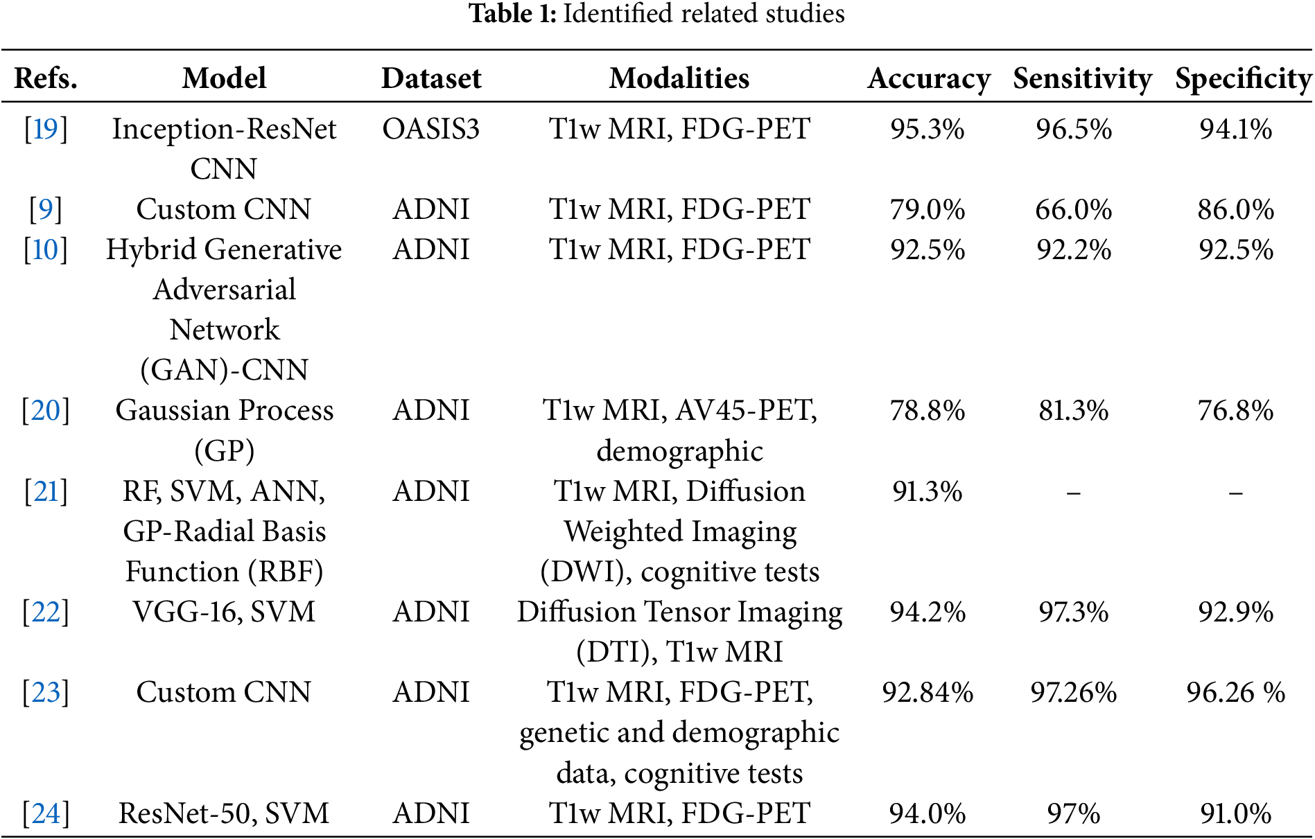
Forouzannezhad et al. [20] used a Gaussian-based method to classify early MCI (EMCI) and late MCI (LMCI) from cognitively normal (CN) patients using the ADNI dataset. They integrated MRI and amyloid AV45-PET with demographic data, focusing on feature fusion from these different sources. In contrast, Rallabandi et al. [19] applied custom CNN architectures such as Inception and ResNet to classify MCI from CN, achieving higher accuracy (95.4%) through the fusion of multiple imaging modalities via Discrete Wavelet Transform (DWT). A similar emphasis on multimodal imaging can be observed in Perez-Gonzalez et al. [21], where T1w MRI and Diffusion Weighted Imaging (DWI) were fused with cognitive tests to perform MCI classification. Their use of various classifiers (RF, SVM, ANN, and Gaussian process classifiers) yielded a peak accuracy of 91.3%, showcasing the impact of diverse feature selection techniques. Kang et al. [22] also employed a fusion-based method using Diffusion Tensor Imaging (DTI) and T1w MRI from the ADNI dataset. However, their approach differed by stacking the image modalities into separate channels. This feature extraction was handled by VGG-16 CNN, followed by classification using an SVM. Although both Kang and Forouzannezhad utilized ADNI, Kang’s emphasis on DTI and VGG-16 contrasted with Forouzannezhad’s Gaussian-based approach and multimodal fusion. Kim et al. [9] explored CNN architectures for MCI detection but adopted a different approach to fusion. Unlike Kang’s stacking technique, Kim did not fuse the T1w MRI and FDG-PET images; instead, they fed these modalities as separate inputs into a custom CNN model. This approach yielded a lower accuracy (79%) compared to Kang and Rallabandi’s higher-performing methods. The concatenation of features at deeper network layers contrasts sharply with other works where fusion happens earlier in the processing pipeline. Chen et al. [23] took the fusion further by integrating T1w MRI, FDG-PET, genetic data, demographic data, and cognitive test results, using a custom CNN to process these diverse inputs. Dwivedi et al. [24] used a fusion strategy similar to Rallabandi’s, applying DWT to T1w MRI and FDG-PET images from the ADNI dataset. They extracted features using ResNet-50 and classified MCI using SVM, achieving 94% accuracy, which approaches Rallabandi’s high accuracy but differs in using the ADNI dataset vs. OASIS3 in Rallabandi’s study. Zhang et al. [10] introduced an innovative approach employing a Generative Adversarial Network (GAN) to generate missing FDG-PET images. They then used a custom CNN for MCI classification, contrasting with Dwivedi’s use of DWT for image fusion. It shows a novel application of GANs in the generation of synthetic data to enhance CNN performance.

Several studies have focused on optimizing the integration of magnetic resonance imaging (MRI) and positron emission tomography (PET) data through innovative network architectures and optimization strategies. For example, study [25] proposed a Pareto-optimized adaptive learning method that uses transposed convolution layers to fuse MRI and PET images. Based on pre-trained VGG networks and morphological pre-processing, this approach demonstrated competitive performance in differentiating stages of AD by effectively capturing cross-modal features. In addition to this strategy, study [26] introduced an image colorization technique paired with a mobile vision transformer (ViT) model. This work uses a Pareto-optimal cosine color map to enhance visual clarity and classification performance across several datasets, including ADNI, AANLIB, and OASIS. Integrating the swish activation function within the ViT architecture further improved the sensitivity and specificity of the model to distinguish various stages of AD. Another line of research has explored the enhancement of image quality before fusion. In [27], the authors demonstrated that applying super-resolution techniques to structural MRI images improves the detection of mild cognitive impairment (MCI). Using advanced loss functions and a Pareto optimal Markov blanket (POMB) for hyperparameter tuning within a generative adversarial framework, the study mitigated common artifacts, such as checkerboard effects. Hence, it improved the perceptual quality of the images used for MCI classification. In addition, study [28] focused on optimizing the convolutional fusion process itself. By varying kernel sizes and employing instance normalization alongside transposed convolution, this approach enhanced the extraction of salient features from heterogeneous MRI and PET data. Evaluated on multiple datasets with metrics such as the Structural Similarity Index Measure (SSIM), the Peak Signal-to-Noise Ratio (PSNR), the Feature Similarity Index Measure (FSIM), and the entropy. The method showed notable improvements in fusion quality, which in turn contributed to higher classification accuracy when integrated with a Mobile Vision Transformer. Extending these fusion techniques to the realm of neural architecture search, study [29] applied Pareto-optimal quantum dynamic optimization to fine-tune the architectural hyperparameters of a Mobile Vision Transformer. Using a static pulse-coupled neural network and a Laplacian pyramid for the initial fusion of sMRI and FDG-PET data, the method achieved robust performance across several evaluation metrics (e.g., PSNR, MSE, SSIM) on standard datasets such as ADNI and OASIS.

3  Materials and Methods

In this study, we have developed a robust model capable of detecting Mild Cognitive Impairment (MCI) by integrating various data modalities. The modalities selected for this model include the following: T1-weighted Magnetic Resonance Imaging (T1w MRI), 11C Pittsburgh Compound-B Positron Emission Tomography (PiB-PET) with the 18F-fluorodeoxyglucose radiopharmaceutical, cognitive test results from the Mini-Mental State Examination (MMSE), Clinical Dementia Rating (CDR) and Functional Activities Questionnaire (FAQ), demographic factors such as years of education and gender, and clinical parameters such as systolic and diastolic blood pressure.

Each modality brings a unique and valuable perspective to the detection process: T1w MRI provides a high resolution structural view of the brain, allowing the detection of cortical atrophy, loss of hippocampal volume, and other neuroanatomical markers associated with MCI and its possible progression to Alzheimer’s disease (AD) [6]. Structural imaging is beneficial for identifying changes in the medial temporal lobe and the entorhinal cortex, regions known to be among the first affected by MCI [30].

PiB-PET reveals metabolism and beta-amyloid plaques in neural tissue. Amyloid accumulation is a key biomarker of the pathology of Alzheimer’s and related dementias and often precedes visible structural or metabolic changes, making PiB-PET a valuable early indicator of MCI. This imaging modality is beneficial for differentiating between amyloid-positive and amyloid-negative individuals, providing information on which patients may progress to AD [6].

Beyond imaging, cognitive assessments such as the Mini-Mental State Examination (MMSE), Clinical Dementia Rating (CDR), and Functional Activities Questionnaire (FAQ) provide important information on individual cognitive function. These standardized tests measure memory, orientation, executive function, and daily living abilities, capturing subtle cognitive impairments that may not yet be evident through imaging alone. Integrating cognitive scores with neuroimaging allows for more accurate classification of MCI, as it accounts for functional deficits that structural and metabolic markers might not fully capture.

Educational level and gender help to account for demographic variations, while blood pressure can reveal any related clinical conditions that can influence cognitive decline. Hypertension is also known to correlate with the progression of MCI [31]. The model can capture vascular contributions to cognitive impairment by incorporating blood pressure data, further enhancing its predictive capabilities. In particular, studies have shown that the treatment of hypertension can slow cognitive decline, reinforcing the importance of integrating vascular health indicators into MCI classification models [32].

The choice of these modalities ensures compatibility across datasets and maximizes the model’s ability to detect early signs of MCI by combining anatomical, metabolic, cognitive, clinical, and demographic data. Through this multimodal approach, the model aims to improve early detection of MCI, which is crucial for timely intervention and personalized treatment planning in clinical settings. Fig. 1 shows a high-level overview of the methodology.

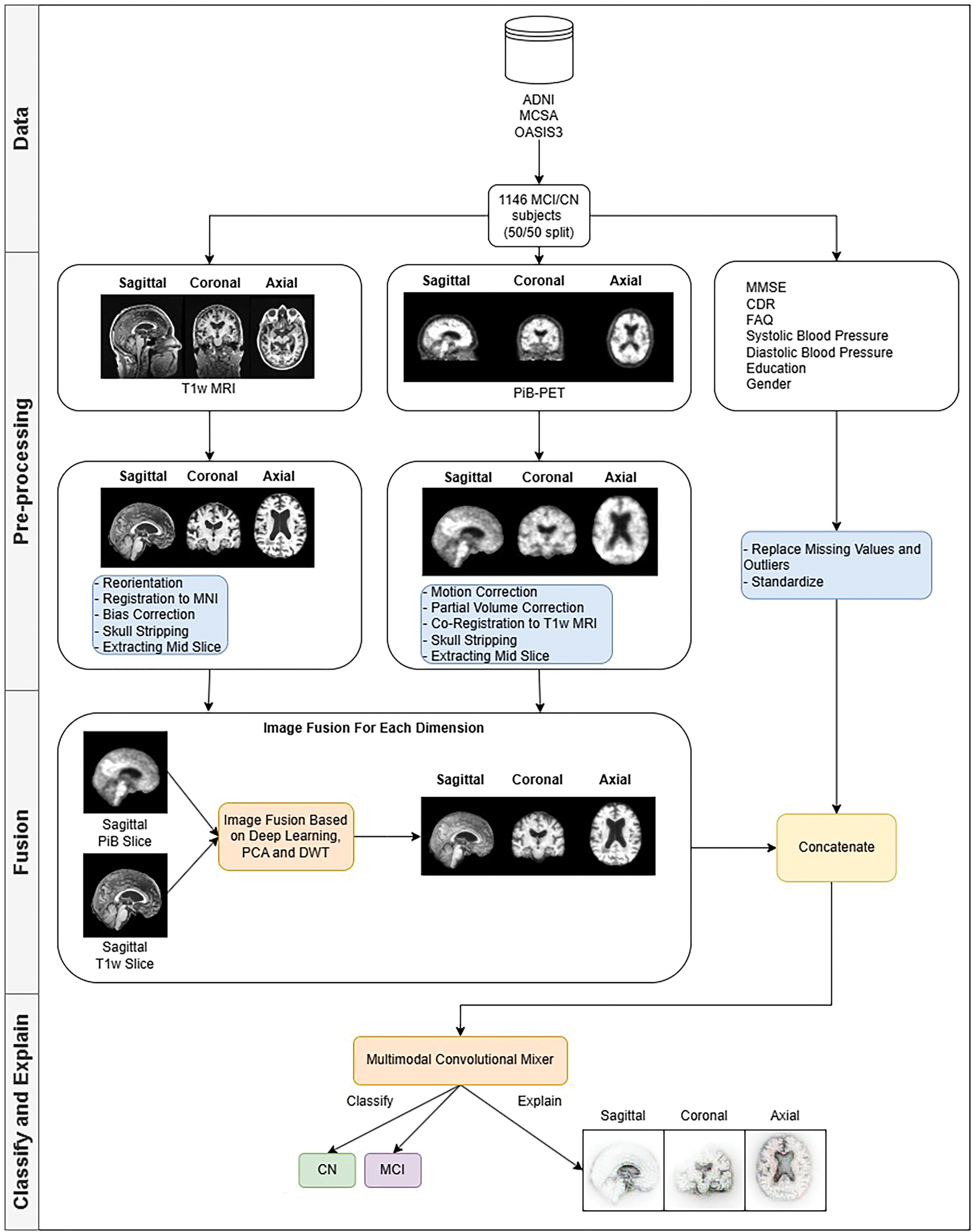
Figure 1: Methodology behind the multimodal convolution mixer in MCI detection

3.1 Dataset

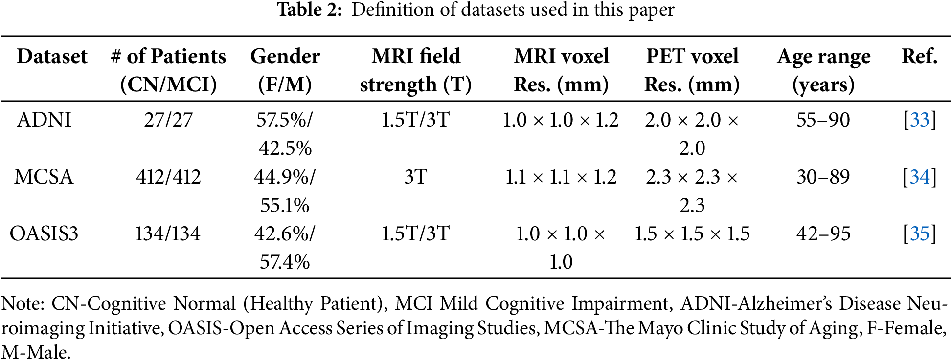
We used three datasets in our study. Alzheimer’s Disease Neuroimaging Initiative (ADNI), The Mayo Clinic Study of Aging (MCSA), and the 3rd edition Open Access Series of Imaging Studies (OASIS3). Table 2 lists the datasets and their respective parameters.

3.1.1 Alzheimer’s Disease Neuroimaging Initiative (ADNI)

ADNI-The study started in 2004 with the primary objective of advancing the understanding of Alzheimer’s disease. The initiative’s core research areas include early detection of Alzheimer’s disease, tracking the progression of cognitive decline, and identifying potential biomarkers for diagnosis and monitoring.

3.1.2 The Mayo Clinic Study of Aging (MCSA)

MCSA-also started in 2004-is another key research initiative aimed at understanding the aging process and the onset of neurodegenerative diseases, particularly dementia. The MCSA focuses on identifying neuroimaging biomarkers that could serve as early predictors of cognitive decline, including Alzheimer’s disease, and understanding the biological changes that occur with aging. One of the main objectives of the study is to develop predictive tools using neuroimaging to diagnose or prevent dementia, which could transform the clinical approach to cognitive disorders related to aging.

3.1.3 Open Access Series of Imaging Studies (OASIS)

OASIS-started in 2007 to provide high-quality, freely available neuroimaging data to researchers studying Alzheimer’s disease and other dementias. By making data publicly accessible, OASIS fosters collaboration and accelerates progress in dementia research. We have used the OASIS3 dataset, a compilation of patient neuroimaging data collected over 30 years with many different structural, functional, and diffusion neuroimaging modalities.

We have merged subjects from different studies into a single dataset to have a greater diversity of patients. Although the number of patients available in the ADNI and OASIS3 datasets with matching modalities was relatively low, a diverse set of patients should promote the generalizability of the method compared to developing it against a single study dataset. The dataset was divided into training and validation sets with a ratio of 85/15.

As shown in Table 2, each dataset differs in terms of scanner specifications, voxel resolution, age, and gender distributions. These factors introduce variability that can affect the generalizability and performance of the model.

Several pre-processing steps were performed for MRI and PET images to overcome potential biases arising from imaging modalities. The pre-processing procedures are explained in Section 3.2. Standard procedures ensure that all imaging modalities can be analyzed under the same conditions, thus minimizing bias toward differences in imaging equipment and signal intensities.

To assess the impact of the variability of the dataset, we have also performed ablation studies that show how much each category of characteristics influences the accuracy of the final model. To check how well the model generalizes given different patient distributions, a 5-fold cross-validation was applied. To check how well the model generalizes given unseen data, Leave-One-Dataset-Out (LODO) cross-dataset validation was used. The results of the ablation study are available in Section 4.6.

3.2 Data Pre-Processing

After merging all the patients into one dataset, we performed pre-processing steps for each data modality group. Tools used in pre-processing are: FSL suite [36]-fslreorient2std (reorientation), flirt (registration and co-registration), fast (bias correction), and slicer (slicing). FreeSurfer suite [37]-mri_synthstrip (skull stripping) [38]. PetSurfer suite [39,40]-mri_gtmpvc (partial volume correction), mri_coreg (motion correction). These specific tools were selected mainly because of previous personal experience. Although there are many other alternatives, the FSL, FreeSurfer, and PetSurfer software suites are industry-tested tools that the research community has used for years (10+). They are more than suitable for this study.

3.2.1 T1w MRI Pre-Processing

The pre-processing steps for T1-weighted Magnetic Resonance Imaging (T1w MRI) include several standard stages to prepare the data for further analysis. The steps performed sequentially are described below:

1.    Reorientation

       First, the images are reoriented into the standard MNI (Montreal Neurological Institute) space, which facilitates alignment with all neuroimaging datasets and ensures consistency between subjects.

2.    Registration

       Following this, the images are registered to the MNI standard atlas, explicitly using the high-resolution MNI152 NLIN 2009b template with a voxel size of 0.5 mm. This registration step allows for a uniform spatial alignment of brain structures across all subjects, accounting for individual variations in brain anatomy.

3.    Bias correction

       Next, bias correction is applied to the images to correct for intensity variance caused by inhomogeneities in the magnetic field, which can distort the images and affect the analysis.

4.    Skull stripping

       Skull stripping removes non-brain structures, such as the skull and surrounding fluids and tissues, ensuring that only the brain is included in subsequent analyses.

5.    Slicing

       Finally, the center slice of the brain volume is extracted to reduce computational complexity and provide a standardized way to detect MCI.

3.2.2 PiB-PET Pre-Processing

The pre-processing steps for 11C Pittsburgh Compound-B Positron Emission Tomography (PiB-PET) images involve several crucial stages to prepare data for the further analysis step. The steps performed sequentially are described below:

1.    The first step is motion correction, which is performed to correct any head movements that may have occurred during the PET scan. PET acquisitions often take several minutes, where even minor head movements can introduce artifacts and distort the alignment of brain structures. Uncorrected motion can lead to blurred images, loss of spatial resolution, and inaccurate quantification of tracer uptake. These distortions are particularly problematic in longitudinal studies or studies with fine-scale regional analysis, where even subtle misalignment can lead to errors in the MCI classification. Motion correction is essential to ensure that the PET image accurately reflects the underlying metabolic activity and tracer distribution to have an accurate and robust diagnostic pipeline.

2.    Partial Volume Correction (PVC) is applied to address the issue of partial volume effects, which occur due to limited spatial resolution and may result in misinterpretation of PET scan images [41]. Since the spatial resolution of PET is much lower than that of MRI, it can lead to signal spillover between adjacent regions, especially in smaller structures in the brain. Without correction, tracer uptake in smaller brain regions may be underestimated due to the mixing of signals from surrounding tissues. By applying PVC, the accurate tracer distribution is better preserved, improving the accuracy of quantitative PET measurements and improving the reliability of further analysis.

3.    Next, the PiB-PET image is co-registered to a corresponding T1-weighted MRI (T1w MRI) scan. This step is critical for aligning the PET data with the high-resolution structural information from the MRI, allowing precise localization of PiB binding in relation to the anatomical regions of the brain. The coregistration process ensures that both imaging modalities are spatially matched, essential for combining the data and performing multimodal analysis.

4.    Skull stripping is then applied to remove non-brain tissues, such as the skull, scalp, and surrounding fluids, irrelevant to brain activity analysis. This step is essential to focus exclusively on the brain regions of interest and eliminate unnecessary noise. By removing non-brain elements, the accuracy of subsequent processing steps, including classification, is improved.

5.    Finally, the mid-slice of the brain is extracted, which provides a representative cross-sectional view of the brain’s structure and PiB distribution. This standardized slicing approach facilitates comparisons across subjects and studies, enabling more consistent analyzes.

3.2.3 Other Modalities Pre-Processing

Other data modalities include the results of cognitive tests, the Mini Mental State Examination (MMSE), the Clinical Dementia Rating (CDR) and Functional Activities Questionnaire (FAQ), education in years and gender, and systolic and diastolic blood pressure. Each of these modalities was carefully processed to ensure data quality. The steps are performed sequentially:

1.    Replacement of missing values

       Missing values were handled by checking if previous visit data was available and using those data as features; otherwise, we replaced missing values with the mean of the respective variable, ensuring minimal bias and preserving statistical integrity.

2.    Handling outliers

       Outliers were replaced with the variable’s mean value. This helps maintain the completeness of the dataset while reducing the impact of extreme values on statistical analyses and machine learning models, thereby improving model robustness and predictive accuracy.

3.    Standardization

       All data was standardized to ensure consistency and comparability between different measures. Standardization was performed by transforming each variable with a mean of zero and a standard deviation of one, using z-score normalization. This step is particularly crucial when combining features with different units of measurement, as it ensures that variables with larger numerical ranges do not disproportionately influence machine learning models.

3.3 Fusion of Different Modalities

After data pre-processing, fusion strategies were applied to the dataset to integrate multiple modalities effectively. Combining T1w MRI and PiB-PET imaging improves the ability to detect MCI using complementary information from different imaging techniques. Structural MRI provides insights into anatomical changes, while PiB-PET highlights changes in metabolic activity. By fusing these modalities, we aim to improve classification accuracy by utilizing more prosperous and diverse data representations. The steps performed sequentially are described below:

1.    Grouping into orthogonal planes

       The first step involved splitting the T1w and PiB-PET image slices into three orthogonal planes: sagittal, coronal, and axial. This approach allows us to analyze each plane separately, as each provides unique information on brain structure and metabolic activity. The sagittal plane (side view) helps visualize asymmetries and atrophy patterns in specific brain regions, such as the medial temporal lobe. The coronal plane (front-to-back view) provides a detailed perspective on loss of hippocampus volume and cortical thinning, which are crucial markers of MCI. The axial plane (top-down view) enables examination of whole-brain connectivity and metabolic activity in different lobes.

2.    Fusion

       Following separation into planes, each set of T1w and PiB-PET image slices from the individual planes were fused using the Deep Image Fusion library [42]. This advanced fusion technique leverages a combination of Principal Component Analysis (PCA), Wavelet Transform, and Deep Learning algorithms to merge imaging data to ensure a low signal-to-noise (SNR) ratio. PCA mainly emphasizes critical structural and functional components while reducing redundant information. Wavelet Transform helps preserve high-frequency details and overall spatial characteristics, improving texture representation. Deep learning fusion ensures that the merged images retain meaningful features while minimizing noise and artifacts.

3.    Feature concatenation

       Once the image fusion process was completed, the fused images were used as input for the Multimodal Convolutional Mixer model. The fused images are used during training, where the image features extracted from the model backbone are concatenated with other data modalities into one feature vector and passed through the classifier to perform MCI detection. More details about the model architecture are available in Section 3.4.

3.4 Multimodal Convolution Mixer

The model backbone is an extension of the ConvMixer architecture [16]. The architecture can be divided into four parts: input embedding, model layers, features preparation, and classifier.

3.4.1 Input Embedding

Input embedding consists of three layers in front of the model (patch embedding, GELU [43] activation, and batch normalization). The fused T1w and PiB-PET images are passed through the patch embedding extraction convolution layer, which essentially uses the same kernel and stride size to calculate the convolution filters in a patch-based manner. Analyzing patches rather than whole images is more computationally efficient. After the computation of patch convolution filters, the output is passed through the GELU activation function, which is used throughout the architecture. We chose GELU since it was used in the original ConvMixer model. Activations are then passed through UncenteredBatchNorm2D modules, which are modified batch normalization layers described in the B-cos network paper [44]. These modules capture batch statistics without the bias term, which accommodates faithfulness in capturing weight contributions.

3.4.2 Model Layers

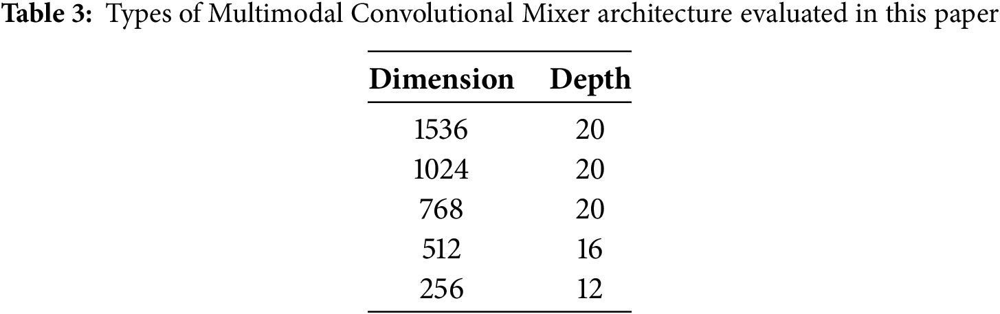
The Multimodal ConvMixer (MCM) layer consists of a residual connection, which skips depth-wise convolution and applies filters for each channel separately. Each convolution module is followed by GELU activation and uncentered batch normalization. The last convolution module in the MCM layer is point-wise, which uses a kernel size of 1 and creates channel-wise dependencies. The MCM layer and depthwise convolution produce efficient convolutions called depthwise-separable [45]. There are n number of layers in the model. MCM-256 uses 12 such layers, MCM-512 uses 16 layers, MCM-768, MCM-1024, and MCM-1536 uses 20 layers.

3.4.3 Features Preparation

Using n number of MCM layers, the output is passed through a global pooling layer and a dropout regularization layer. Global average pooling is a critical downsampling technique that reduces the spatial dimensions of feature maps while retaining essential information. Dropout regularization improves generalization by randomly setting some neuron activations to zero during training. This forces the network to learn more robust and distributed feature representations rather than relying on specific activations, thus improving computational efficiency and mitigating overfitting.

Finally, the extracted feature maps are flattened and fed into a multi-head self-attention module, a transformative mechanism originally popularized in Natural Language Processing (NLP) but now playing an equally crucial role in computer vision. Multi-head self-attention enables the model to dynamically attend to different regions of an image, learning relationships between various objects or object parts. Unlike traditional convolutional layers, which rely on localized receptive fields, self-attention mechanisms capture global dependencies, allowing the network to understand how different parts of an image interact, even at long distances.

This mechanism is frequently used in Vision Transformers (ViTs) [46–48], where it replaces convolutions to provide a more flexible and context-sensitive approach to feature extraction. Each attention head in the multi-head framework learns different aspects of the input data, such as texture, shape, or positional relationships, enabling richer feature representations. This makes multi-head self-attention useful for complex vision tasks such as object detection, image segmentation, and fine-grained classification, where understanding local and global structures is crucial.

3.4.4 Classifier

The output of the multi-head self-attention module is then concatenated with numeric features (cognitive tests, demographics, etc.) that are prepared in a vector format. The final feature vector is then fed into a custom Multi-Layer Perceptron (MLP) classifier, ready for linear (fully connected) layers, followed by GELU activation functions. We also use dropout regularization in this classifier to further enhance the robustness to overfitting. The feature vector fed into the classifier head was down-sampled four times and finally reduced to a binary classification result of Cognitively Normal (CN) or Mild Cognitive Impairment (MCI).

We have replaced the original convolution and batch normalization layers with the B-cos modules described in [44]. The convolution modules (Conv2D) and batch normalization (UncenteredBatchNorm2D) of the B-cos networks allow the visualization of the highest contributing features during inference. They work similarly to Grad-CAM [49] or, in the case of numerical features, SHAP values [50]. We chose B-cos modules over Grad-CAM because of several reasons: faithfulness, with B-cos networks replacement of layers in models, is necessary, and these layers capture summaries of all computations during training; they also capture both positive and negative contributions, which leads to more detailed and focused explanations, where Grad-CAM is a post-hoc computation and it may not be faithful to the network’s internal computations; high quality, clearly focused contributions, Grad-CAM captures saliency maps of gradients backpropagated through the network and only highlights the regions in the images, that contribute most to the prediction, but usually are coarse and noisy, where B-cos provides focused and clear contribution maps, that are easier to interpret. An example of Grad-CAM vs. B-cos feature contribution maps is shown in Fig. 2.

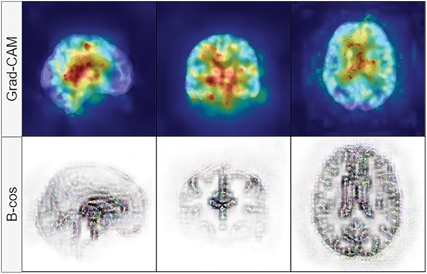
Figure 2: Visual comparison between Grad-CAM (top row) and B-cos (bottom row) feature contribution maps. B-cos explanations are more focused, where Grad-CAM provides a high-level overview of the region that contributes the most in classification

Other changes include the addition of regularization with the dropout module; multi-head self-attention, which allows the model to learn features from different subspaces [51]; a custom Multi-Layer Perceptron (MLP) classifier head, which effectively classifies concatenated multi-modal features into Cognitively Normal (CN) and Mild Cognitive Impairment (MCI). The complete model architecture is depicted in Fig. 3.

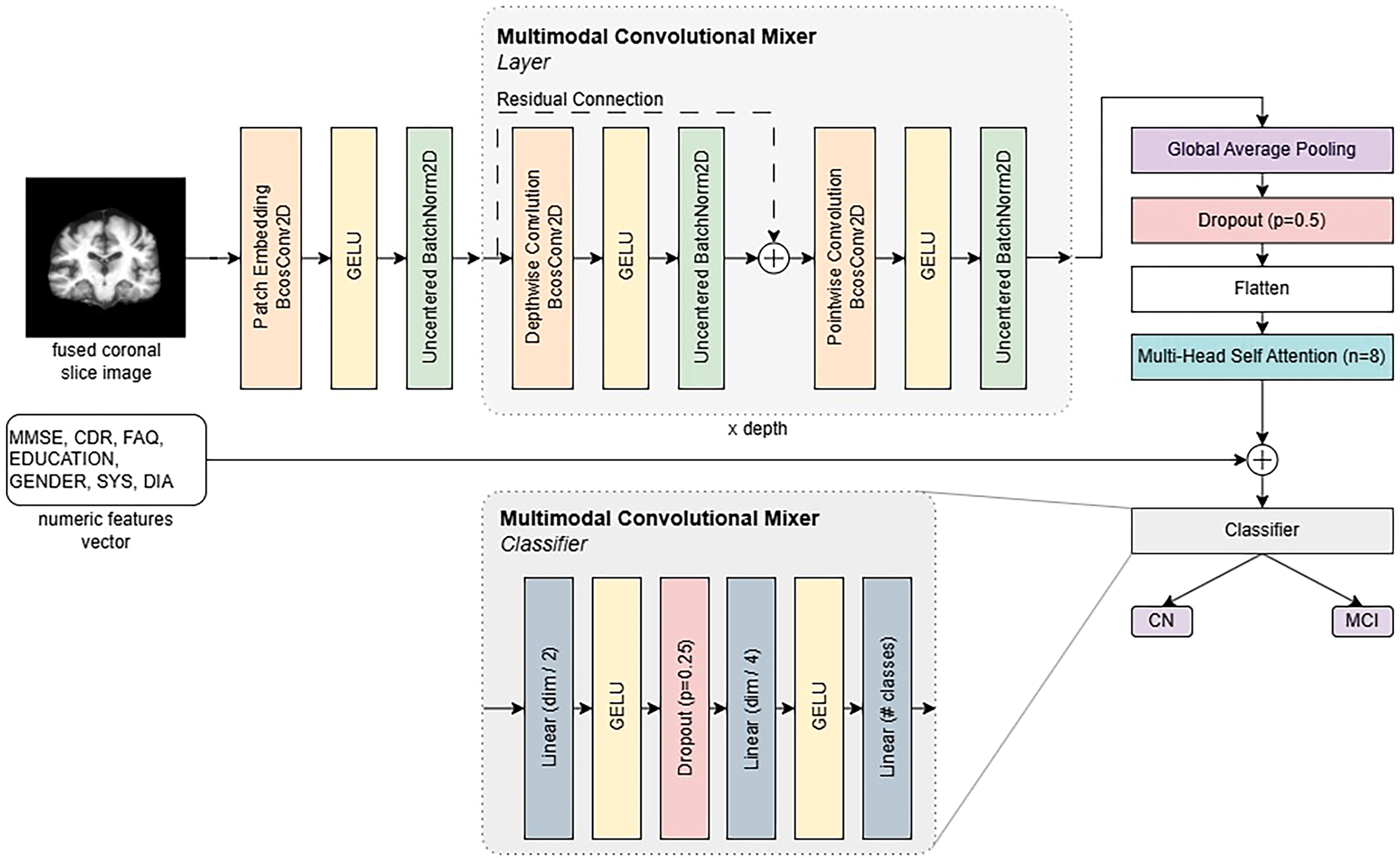
Figure 3: Multimodal convolution mixer architecture

3.5 Evaluation of Results

To assess the classification performance of the proposed model, we employ commonly used metrics: accuracy, sensitivity, specificity, and Matthews Correlation Coefficient (MCC). These metrics provide a comprehensive evaluation by measuring overall correctness, the ability to detect positive cases, and the ability to exclude negative cases. Definitions and mathematical formulations are provided in the list below:

•   Accuracy is the proportion of correctly classified instances among all predictions. It reflects the overall performance of the model.

Accuracy=1N∑iN1(yi=y^i)(1)

•   Sensitivity is the proportion of actual positive cases correctly identified by the model. It represents the true positive rate, crucial in applications where missing a positive instance has serious consequences.

Sensitivity=TPTP+FN(2)

•   Specificity is the proportion of actual negative cases correctly identified by the model. It represents the true negative rate and ensures that negative cases are not misclassified as positives.

Specificity=TNTN+FP(3)

•   Matthews Correlation Coefficient (MCC) is a balanced measure that considers true and false positives and negatives. It considers all four confusion matrix categories and returns a value between –1 and +1. An MCC of +1 indicates perfect prediction, 0 indicates random prediction, and −1 indicates total disagreement between prediction and observation.

MCC=TP×TN−FP×FN(TP+FP)(TP+FN)(TN+FP)(TN+FN)(4)

4  Results

4.1 Implementation Details

The experiments were performed on a desktop computer with an AMD Ryzen 5900X Central Processing Unit (CPU), RTX 4090 Graphics Processing Unit (GPU), and 32 GB RAM.

All models were trained with a batch size of 16 since this was the only batch size fitting into GPU memory. We used a cosine annealing learning rate scheduler with a learning rate range [2−5;1−7], Adam optimizer with weight decay of 1−3 and a Binary Cross Entropy (BCE) loss for classification.

4.2 Results of Multimodal Convolution Mixer

To evaluate our proposed method, we have trained a variety of methods: ResNet family networks [52], DenseNet 121 and 201 [53], four different Vision Transformers [46] (tiny, small, base and large), MobileNet4 [54] and baseline Convolutional Mixer (ConvMixer) networks [16]. We explored five different architecture versions of ConvMixer as described in Table 3. All models used eight heads in the self-attention module, a kernel size of 9, and a patch size of 7 since these parameters showed the best results across models.

4.3 Classification Results with MCSA Dataset

All models were trained on individual scan planes (sagittal, coronal, and axial) to see how representative each plane is regarding MCI detection. First, we evaluated model performance on the biggest dataset we acquired-Mayo Clinic (MCSA). It was nonsensical to assess the ADNI and OASIS3 separately due to their size. It would overfit both datasets due to high variance. However, we provide Leave-One-Dataset-Out (LODO) cross-dataset validation and 5-fold cross-validation results in the ablation studies subsection. Classification results using the MCSA dataset on the sagittal plane are listed in Table 4.

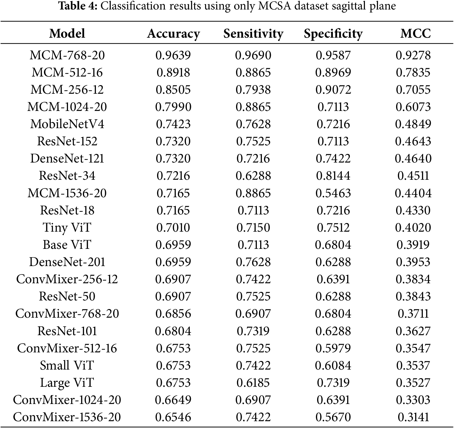
4.3.1 Classification Results with MCSA Dataset in Sagittal Plane

With the MCSA dataset in the sagittal plane, the highest achieved accuracy is 96.3%, sensitivity 96.9%, specificity 95.87%, and MCC 0.9278 by our proposed MCM model, which uses 768 dimension convolution filters. In the sagittal plane on the MCSA dataset, only the MCM-1536 model shows moderate performance, similar to other baseline models; however, all other MCM models outperform the baseline by around 5%–20%. During training, it was obvious that most of the baseline models were suffering from overfitting since the training BCE loss diverged from the validation loss. Utilizing dropout modules for regularization, both in the backbone of the MCM model and in a classifier, allowed our proposed method to cope with high variance in the dataset.

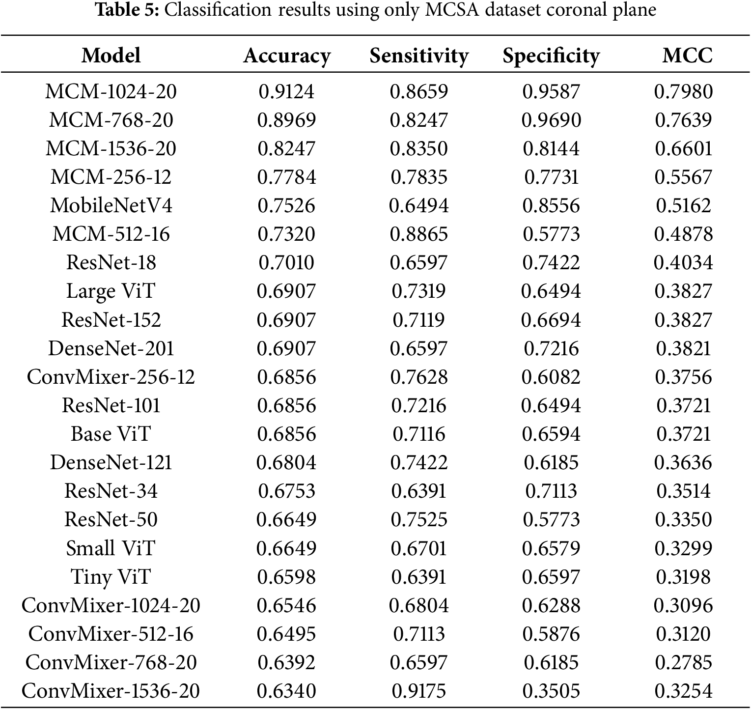
4.3.2 Classification Results with MCSA Dataset in Coronal Plane

The classification results with the MCSA dataset in the coronal plane are listed in Table 5. Compared to the sagittal plane, the highest achieved accuracy is lower −91.24% compared to 96.3%. However, most models show slightly worse performance. Compared to the sagittal plane, the MCM-1024 model shows the best results, with MCM-768 falling behind 2% in accuracy. The results show that using the MCSA dataset in the coronal plane, the classification is not as accurate, and the sagittal plane is a better choice for MCI detection.

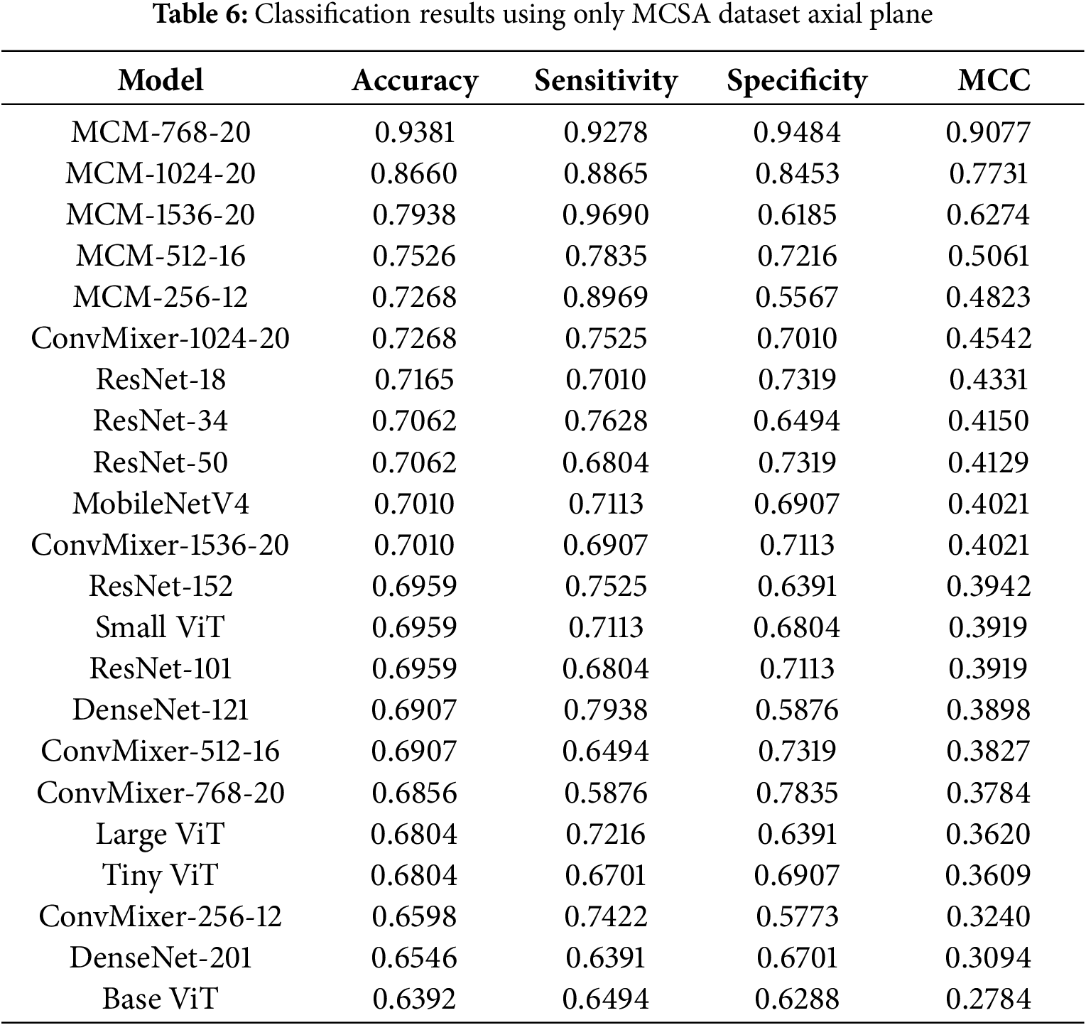
4.3.3 Classification Results with MCSA Dataset in Axial Plane

The classification results with the MCSA dataset in the axial plane are listed in Table 6. We can see that all MCM models outperform the baseline, where the best results are achieved by the MCM-768 and MCM-1024 models, with the highest accuracy being 93.81%, 92.78% sensitivity, 94.84% specificity and MCC 0.9077. The MCM-768 model achieved 3% lower accuracy than the sagittal plane, compared to the coronal plane, which achieved 2% higher accuracy. These results show that the sagittal and axial planes are the most descriptive with respect to the differentiation of patients with MCI vs. CN using the selected image and non-image modalities in the MCSA dataset.

4.4 Classification Results with Full Dataset

The second part of the evaluation was to check whether the proposed method can generalize with various datasets; therefore, we combined all patients from the ADNI, MCSA, and OASIS3 datasets into one and then performed the same experiments with the MCSA dataset. Table 7 lists the results in the sagittal plane.

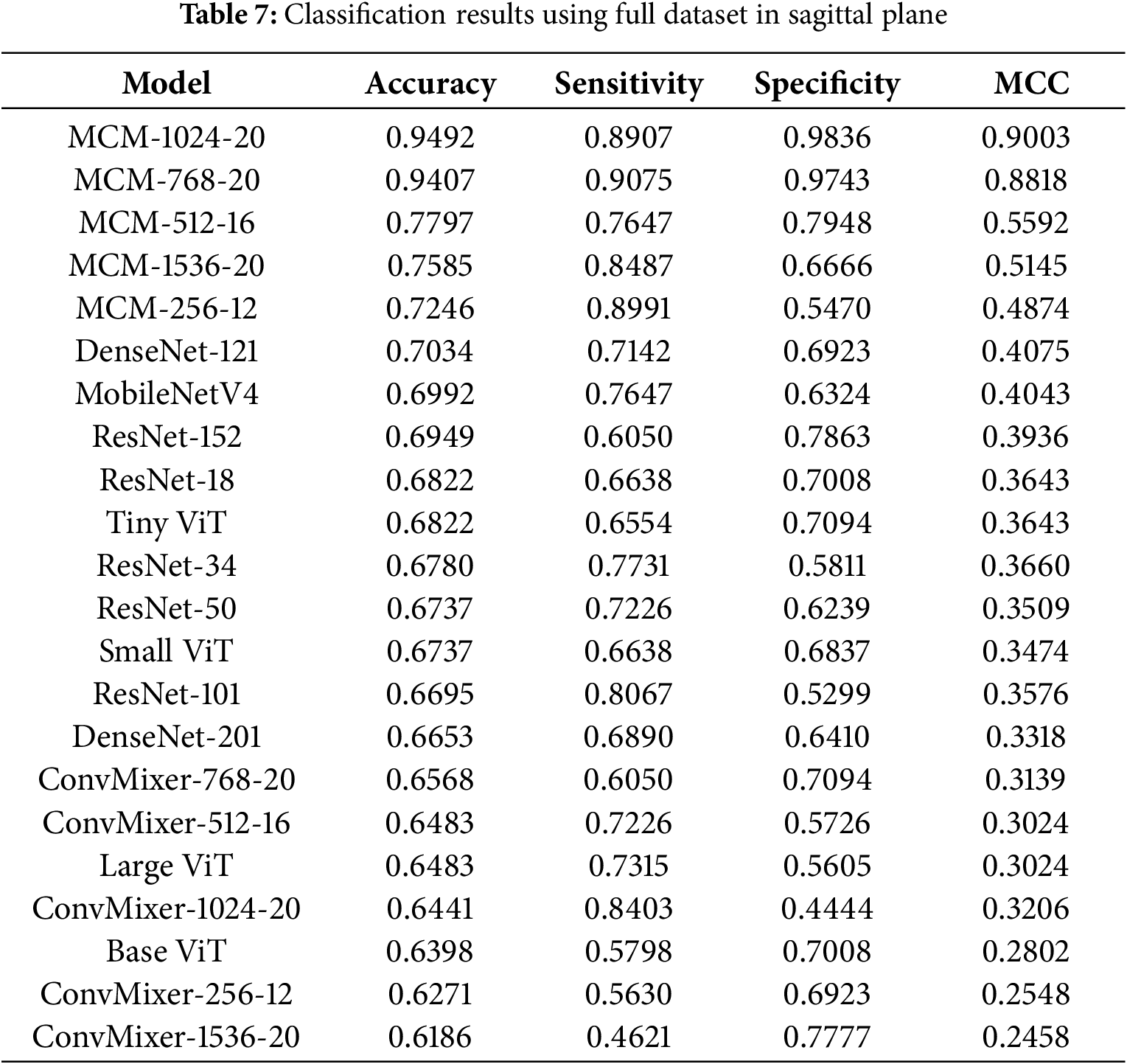
4.4.1 Classification Results with Full Dataset in Sagittal Plane

Our proposed MCM-1024 method can reach 94.92% accuracy, 89.07% sensitivity, 98.36% specificity, and 0.9003 MCC. The MCM-1024 and MCM-768 show good results, although the balance between sensitivity and specificity could be better. These two metrics should match, meaning that the model is equally likely to predict MCI or CN. In this case, models tend to predict more likely CN. Interestingly, the baseline ConvMixer models show relatively low performance, which means that using regularization techniques with self-attention and custom classifier allows not only to reduce overfitting but also to improve classification performance by 10%–20%.

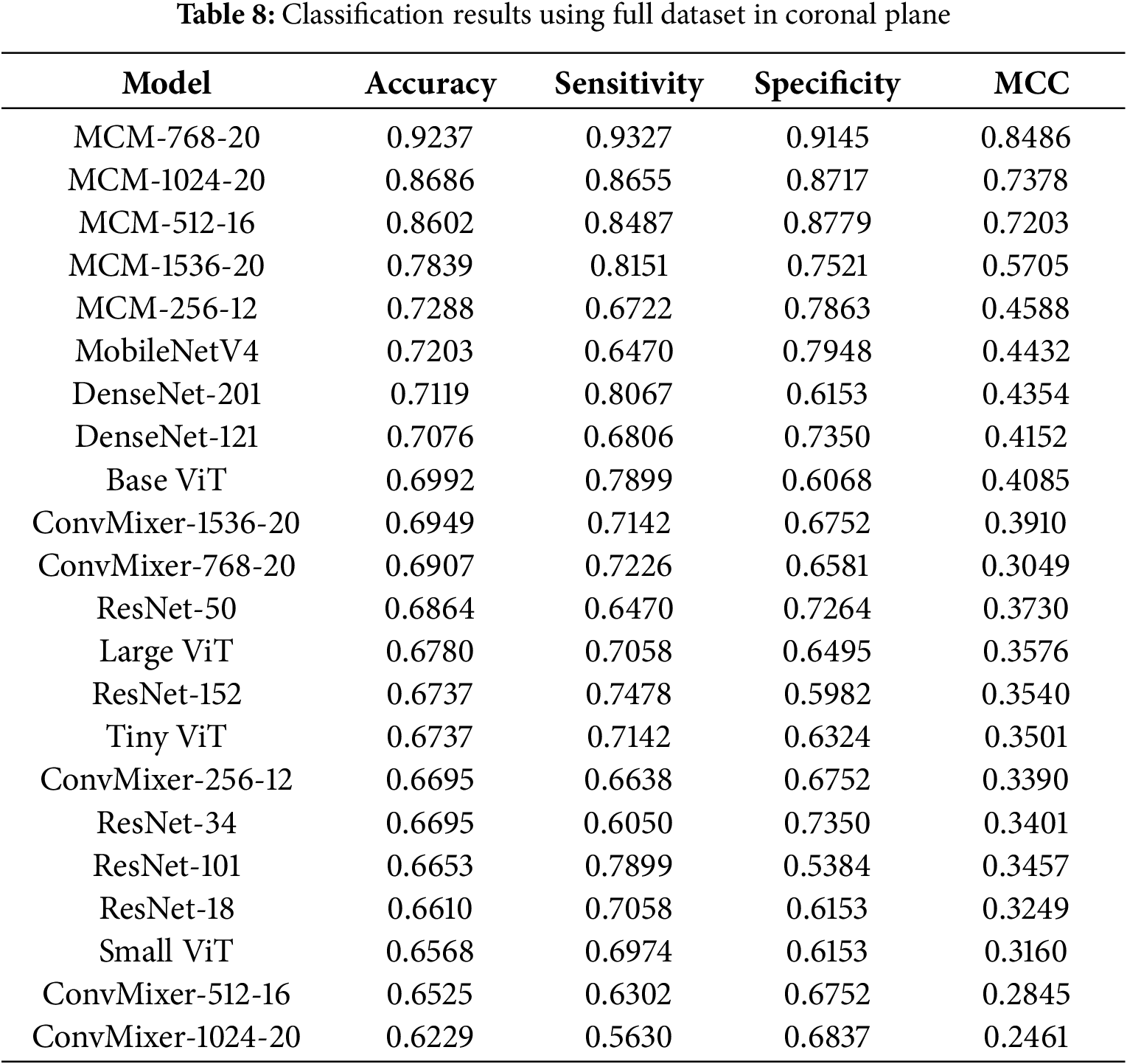
4.4.2 Classification Results with Full Dataset in Coronal Plane

The classification results with the full dataset in the coronal plane are listed in Table 8. Here, we can see that the MCM-256 model is only slightly better than the MobileNet4 baseline, and the best model overall is MCM-768, achieving 92.37% accuracy, 93.27% sensitivity, 91.45% specificity, and 0.8486 MCC. In this case, there is an excellent balance between sensitivity and specificity, which means the model is not biased toward choosing the diagnosis of MCI or CN. Again, all MCM models outperform the tested baseline models.

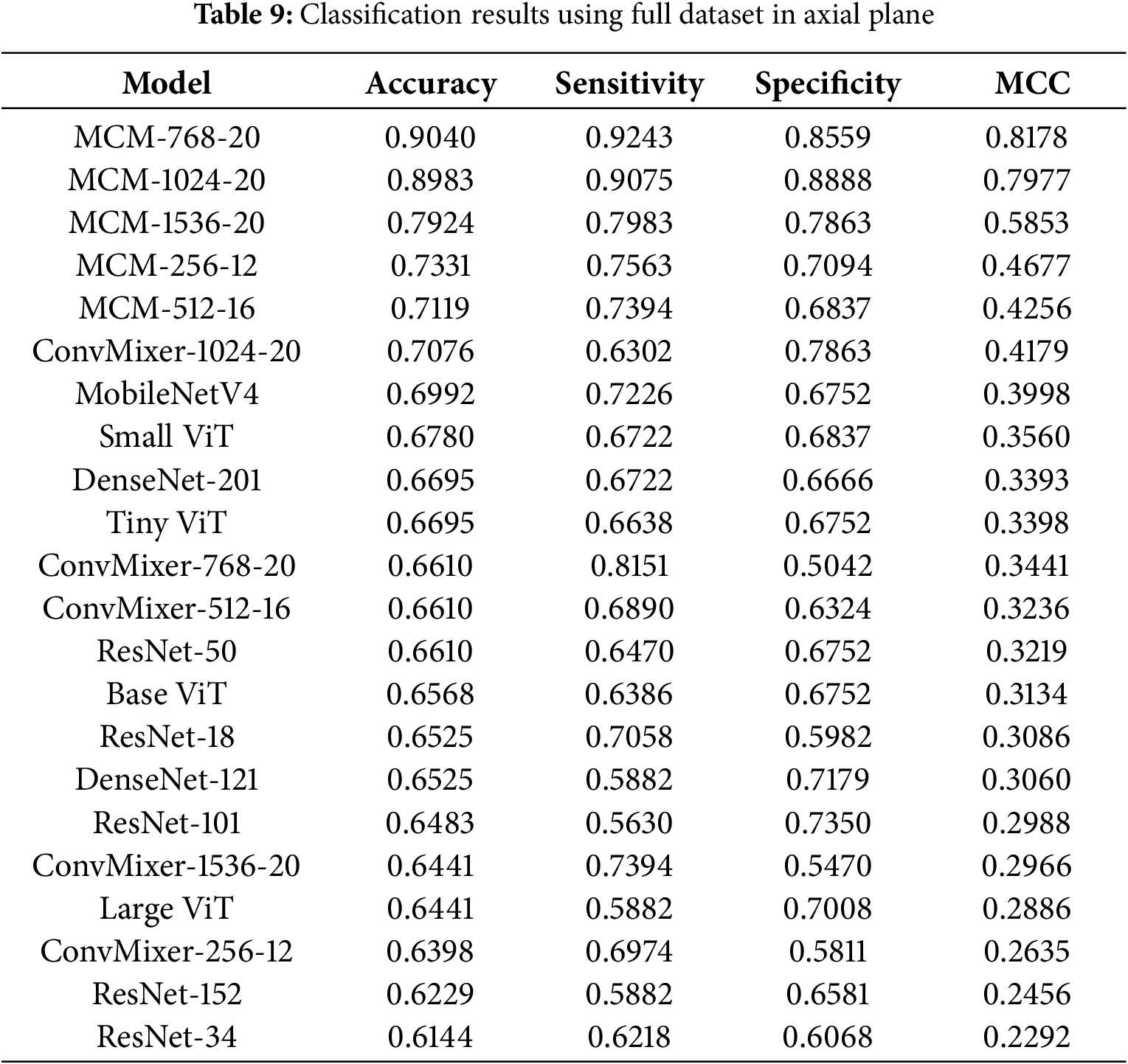
4.4.3 Classification Results with Full Dataset in Axial Plane

The classification results with the full dataset in the axial plane are listed in Table 9. MCM-768 achieved the highest accuracy at 90.4%, 92.43% sensitivity, 85.59% specificity, and 0.8178 MCC. The axial plane using a full dataset shows the lowest accuracy achieved compared to other planes. Compared to results only using the MCSA dataset, we can see that the performance on the sagittal plane remains the best. Still, the coronal plane results are slightly worse using the full dataset. This means that the ADNI and OASIS3 datasets in the axial plane introduce more variance, and therefore the models do not capture high-quality differentiating features due to apparent noise. Overall, MCM models using the full dataset in the axial plane still outperform all baseline models tested.

In summary, in almost all scenarios tested, all MCM models outperformed the baseline models by 10% on average (1%–20% at extremums). The proposed method, particularly the MCM-768 variant, shows great MCI classification results in the MCSA dataset, but it can also generalize well on mixed datasets.

4.4.4 Summary of Model Performances

To provide a comprehensive and representative evaluation of model performance, Table 10 and Fig. 4 summarize key metrics–accuracy, sensitivity, specificity, and MCC–averaged over the sagittal, coronal, and axial planes using only the full dataset (which includes MCSA).

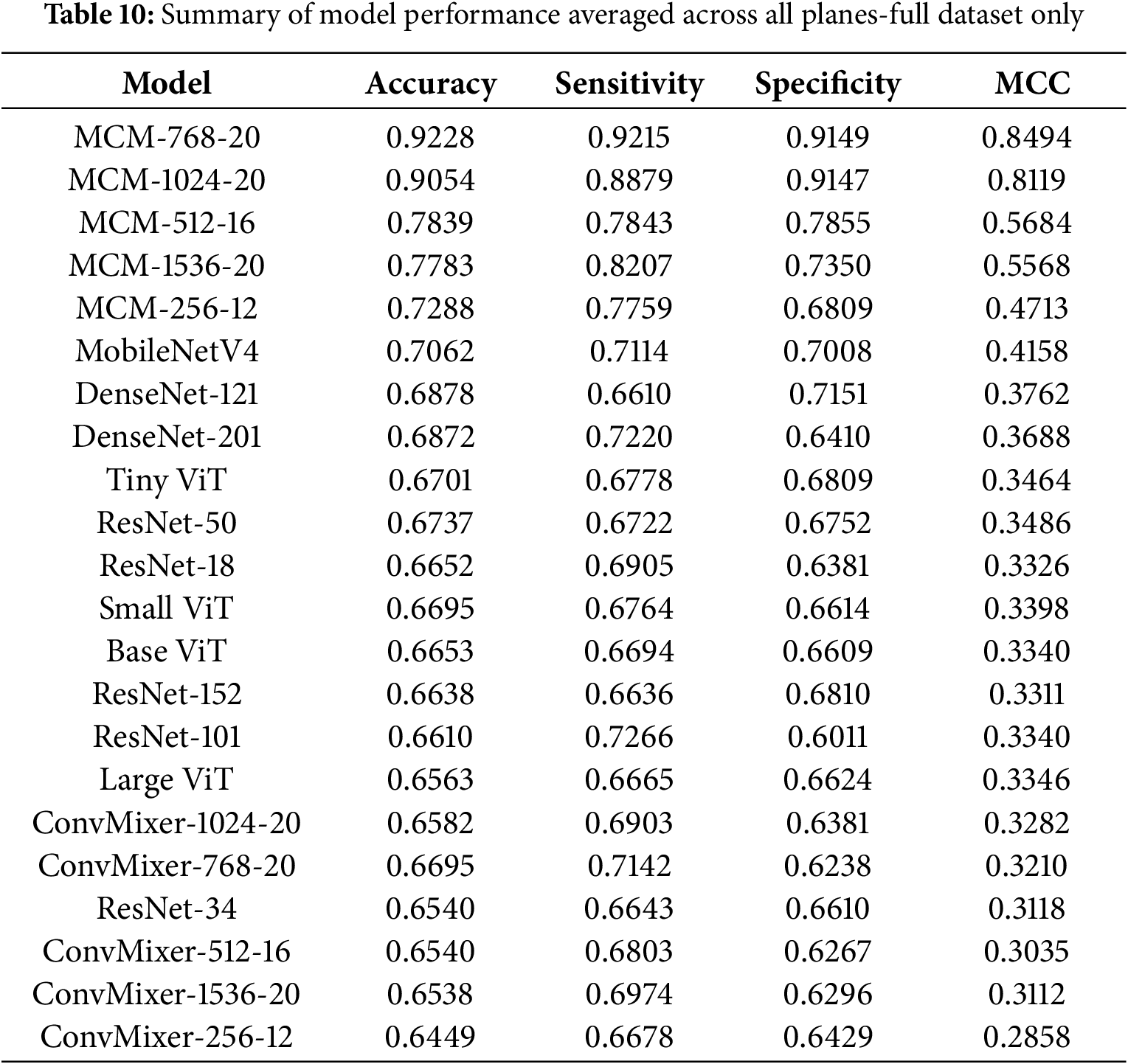
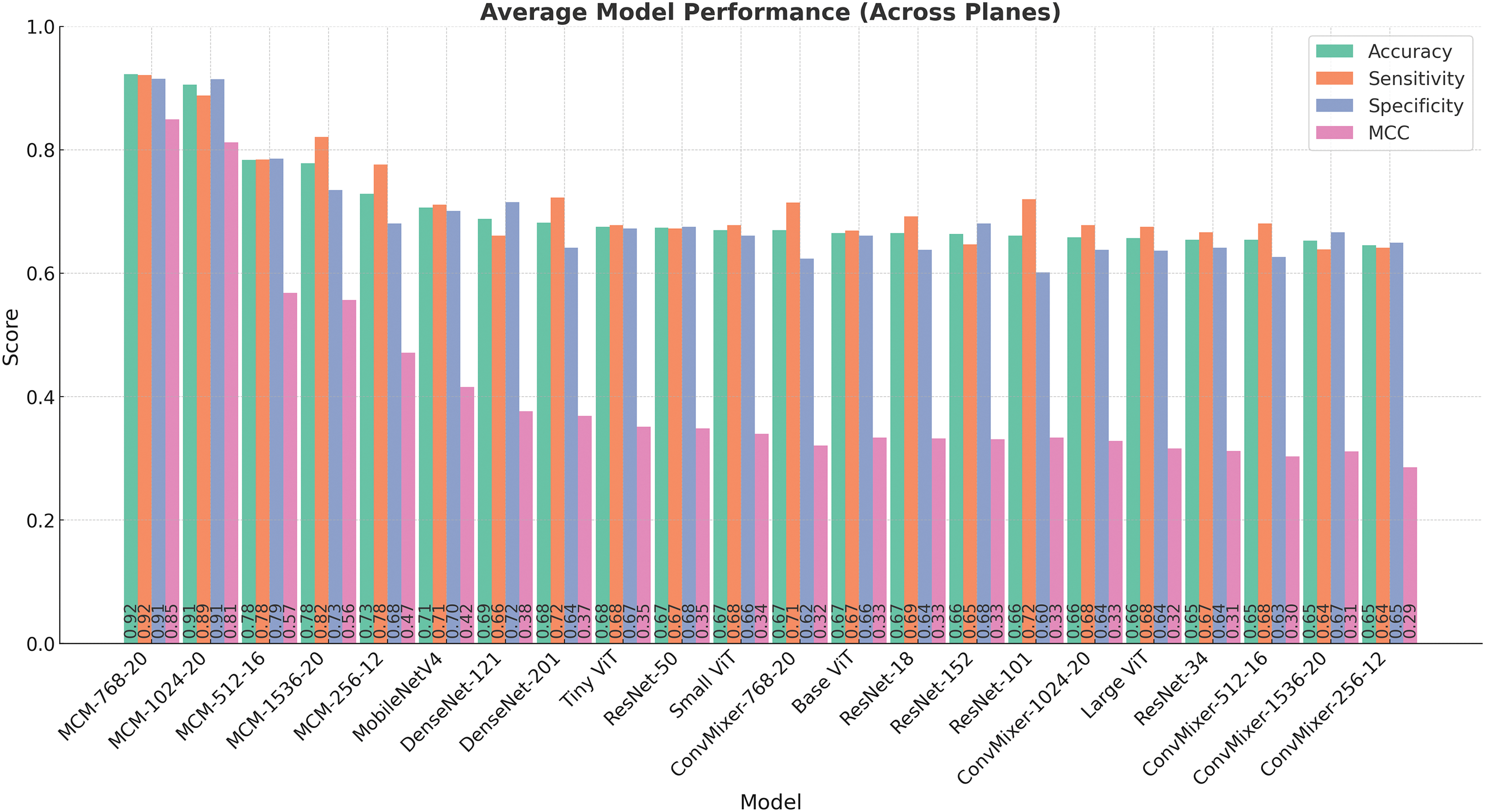
Figure 4: Comparison of model performance metrics (accuracy, sensitivity, specificity, and MCC) averaged over all orthogonal planes (sagittal, coronal, and axial)

Table 10 presents a list of models sorted by the average accuracy. The highest-performing model, MCM-768, achieves an average accuracy of 92.28%, coupled with a high sensitivity of 92.15%, specificity of 91.49%, and MCC of 0.8494, demonstrating robust discriminative ability. Other MCM variants, such as MCM-1024 and MCM-512, also perform strongly on all metrics, further strengthening the effectiveness of the proposed architecture.

Models like MCM-512, MobileNetV4, and several DenseNet, ResNet, and ViT variants demonstrated moderate performance. Accuracy for these models ranged from around 66% to 78%, and MCC values ranged from 0.33 to 0.57. Although some showed a balance between sensitivity and specificity, their overall reliability, as reflected by the MCC, was notably lower than that of the leading MCM models.

The bar chart in Fig. 4 visually complements the table by illustrating the performance of each model across the three metrics. For example, while MCM-1536 demonstrates high sensitivity 82.35%, it exhibits lower specificity 73.50%, suggesting a tendency to over-predict positive cases. In contrast, some models, such as MobileNetV4 and TinyViT, show balanced but moderate performance, indicating their potential for further optimizations.

The baseline ConvMixer models consistently showed lower performance in all metrics, with MCC values mostly below 0.33. Interestingly, increasing the size of these models (e.g., from ConvMixer-256 to ConvMixer-1536) did not lead to meaningful improvements. This indicates that the ConvMixer architecture, without our proposed changes, is not suitable for the MCI classification task with the complete dataset.

4.5 Visualization of the Most Contributing Features

To gain deeper insights into the decision-making process of our model, we conducted an additional study by replacing convolutional and batch normalization layers in the MCM architecture with B-cos modules [44]. These modules facilitate the generation of feature contribution maps, offering enhanced interpretability by visualizing which regions in the input images most strongly influence the model’s predictions.

The figures in this subsection present selected visualizations of the most contributing features in different orthogonal planes–sagittal, coronal, and axial–using fused T1w and PiB-PET images. These visualizations help uncover spatial patterns that differentiate CN individuals from those with MCI and are aligned with known clinical markers of early cognitive decline.

4.5.1 Sagittal Plane

Fig. 5 displays the feature contribution maps for the sagittal plane. For MCI subjects, the most notable features are concentrated around midline structures such as the corpus callosum, the thalamus, and the lateral ventricles. These areas are consistent with clinical observations that report structural and metabolic changes in these regions in the early stages of cognitive impairment [55–58]. In subjects with CN, while attention is still partially focused in the brain’s core, the model also focuses on the curvature and width of the cerebral cortex, suggesting a role for cortical thickness and brain volume - both recognized as valuable indicators in neurodegenerative processes.

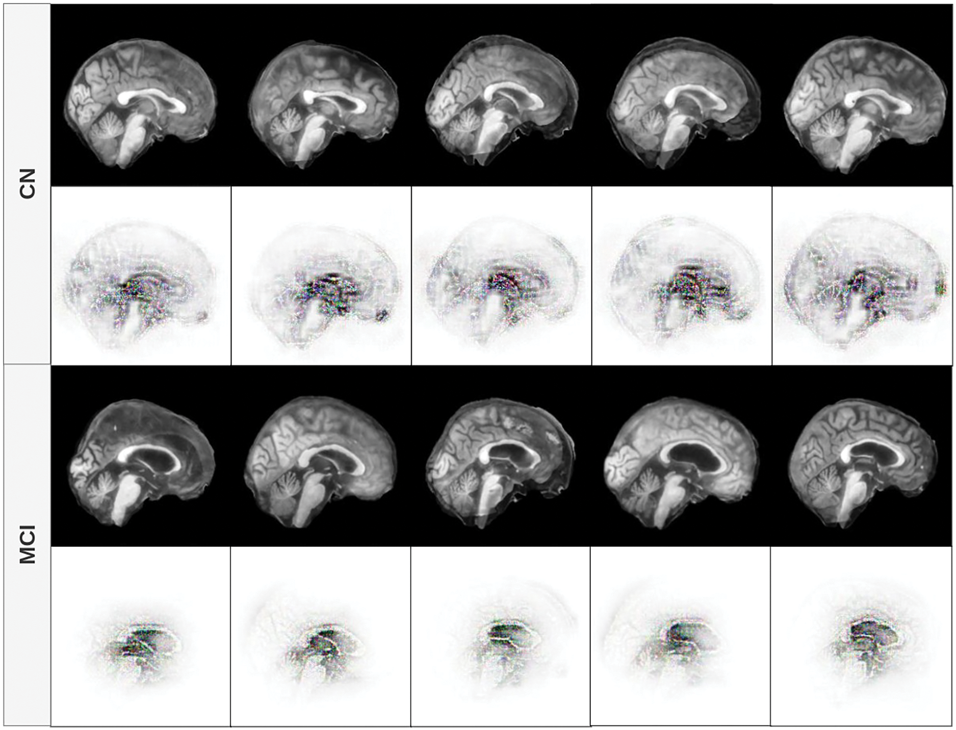
Figure 5: Feature contribution visualization in the sagittal plane. The model highlights midline brain structures (corpus callosum, thalamus, ventricles) for MCI subjects, while CN cases emphasize cortical curvature and volume

4.5.2 Coronal Plane

In Fig. 6, we observe that the focus of the model for patients with MCI remains concentrated in the central region of the brain, particularly the lateral ventricles and surrounding white matter. This aligns with the findings that ventricular enlargement and white matter changes are early biomarkers of MCI. For CN cases, the model continues to focus on both central structures and peripheral cortical boundaries, again indicating that preserved cortical morphology is a distinguishing feature in cognitively normal aging [59].

Figure 6: Feature contribution visualization in the coronal plane. The model’s attention for MCI subjects centers around the lateral ventricles and white matter, while for CN cases, it also includes cortical boundaries and overall brain shape

4.5.3 Axial Plane

Fig. 7 presents the axial view. In MCI subjects, consistent with the other planes, the highest contributions are observed in the central ventricular regions. In contrast, CN subjects show model attention primarily directed toward the outer edges and sulci of the brain. This again suggests that the structural integrity of the cortical surface and brain volume play a key role in the distinction of CN from MCI, reinforcing well-established neuroimaging findings.

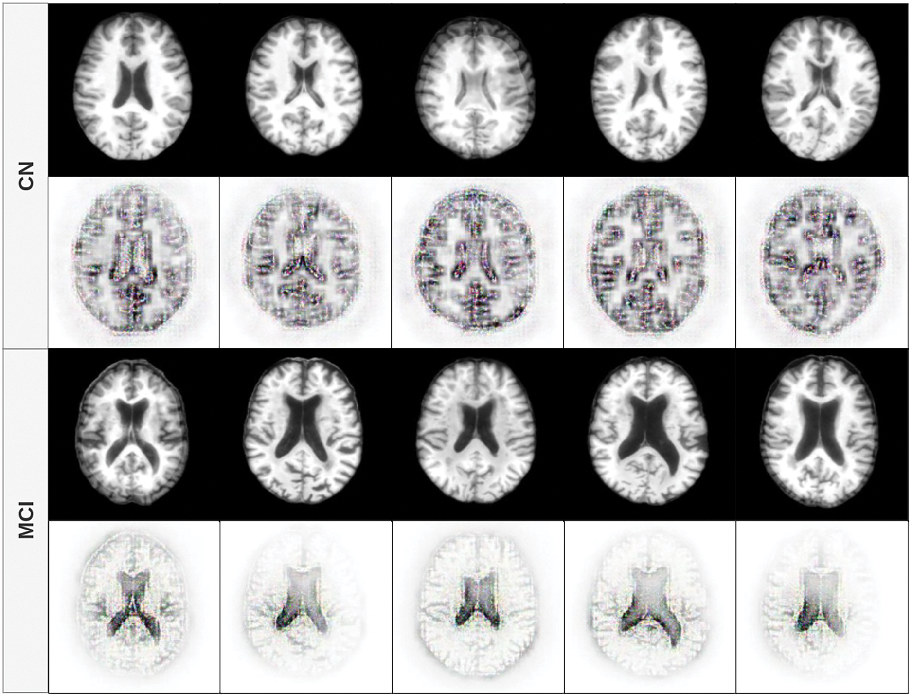
Figure 7: Feature contribution visualization in the axial plane. MCI cases show attention in central regions, especially the lateral ventricles, while CN subjects have contributions from the cortical edges and sulcal patterns

4.5.4 Interpretation and Clinical Relevance

Across all planes, a consistent pattern emerges: in MCI cases, the model focuses on central brain regions, especially the lateral ventricles and midline structures, likely reflecting early neurodegenerative changes such as atrophy and ventricular enlargement. In contrast, CN cases draw attention to both central and peripheral areas, particularly the cortical boundaries, suggesting that the model is sensitive to preserved cortical morphology and brain volume, which are protective factors against cognitive decline.

These visual patterns support the model’s ability to align its learned representations with clinical knowledge, providing interpretability and trust in its predictive mechanisms. Future work could include quantitative analysis of these attention maps and comparison with expert-labeled regions of interest to validate the model’s focus areas further.

4.6 Ablation Studies

4.6.1 Influence of Multi-Head Self-Attention Module

We performed ablation studies to check the influence of the multi-head self-attention module on the network. We performed the same experiments with our proposed model, the only difference being that we removed the multi-head self-attention module.

MCSA Dataset

The classification performance of MCM models without multi-head self-attention on the MCSA dataset across sagittal, coronal, and axial planes is summarized in Table 11. Compared to baseline models, the results show moderate differences, with improvements of approximately 2% in accuracy for the sagittal plane when using the MCM-1024 model. However, these improvements are lower than those observed when incorporating multi-head self-attention, indicating its contribution to enhancing performance.

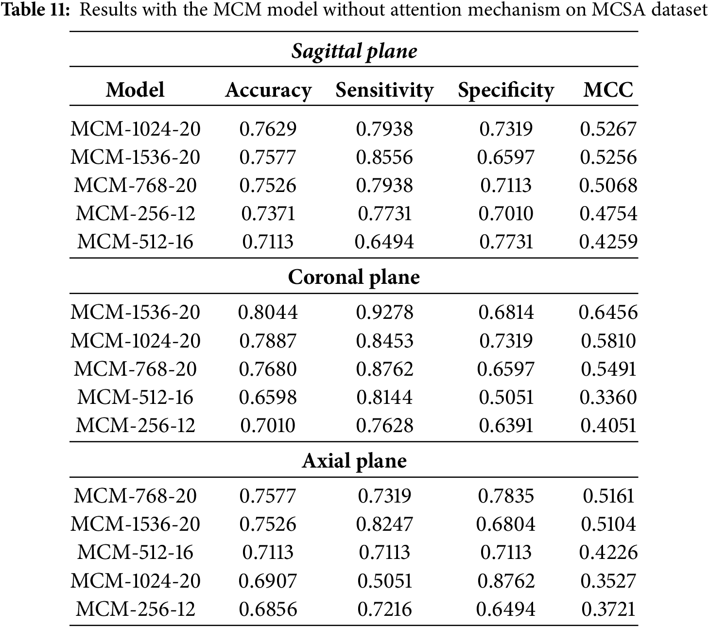
The MCM-1024 model achieves the highest accuracy in the sagittal plane, at 76.29%. However, sensitivity and specificity remain relatively balanced, at 79.38% and 73.19%, respectively. We see moderate performance when compared to the MCC metric. Compared to models that incorporate attention mechanisms, the overall classification performance is marginally improved over baseline models but does not exhibit a substantial boost.

In the coronal plane, the MCM-1536 model achieves the highest accuracy at 80.44%, with a strong sensitivity of 92.78% but low specificity at 68.14%. The high sensitivity implies that the model is effective in detecting MCI cases. However, the low specificity suggests a higher rate of false positives, which means it struggles to classify healthy patients correctly. Compared to results using multi-head self-attention on the full dataset, the relative improvement over the baseline is approximately 8%, and with MCSA alone, the improvement is around 5%. This highlights the impact of the removal of self-attention by multiple heads, which reduces the ability of the model to maintain specificity, potentially leading to an increased false positive rate in clinical applications.

For the axial plane, classification performance declines more noticeably without multi-head self-attention. The MCM-768 model achieves the highest accuracy at 75.77%, but overall, the results indicate a drop of approximately 4%–18% compared to the attention-enhanced models. This suggests that the axial plane benefits more from the additional feature extraction capabilities provided by self-attention, potentially due to the complexity and variability in feature representation in this plane.

Full Dataset

The classification results for MCM models without multi-head self-attention on the full dataset (MCSA + ADNI + OASIS3) are listed in Table 12. Compared to models trained solely on the MCSA dataset, these results demonstrate the effect of increased dataset variability on model performance. While some models achieve comparable accuracy, the sensitivity-specificity balance is affected, particularly in the sagittal and coronal planes. In addition, all models show moderate classification performance, as indicated by the MCC metric.

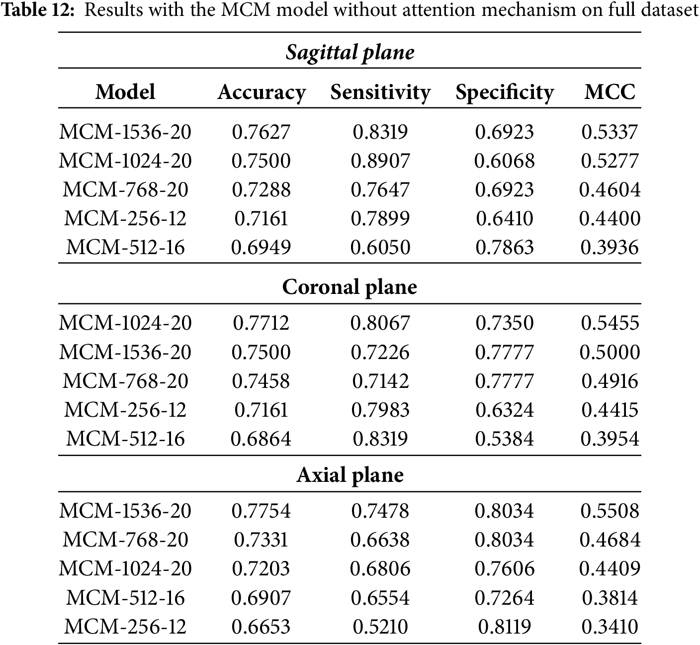
Only the MCM-1536 model maintains a comparable accuracy (76.27%) to its MCSA-trained counterpart in the sagittal plane. However, its sensitivity (83.19%) is slightly higher at the cost of specificity (69.23%), indicating a greater tendency toward detecting positive cases at the expense of more false positives. All other model variations show a general decrease in performance, with the accuracy dropping below 75%. This suggests that the additional variability introduced by the full dataset makes it more challenging for models without self-attention to generalize well.

For the coronal plane, the highest accuracy achieved is 77.12% with the MCM-1024 model. Compared to baseline models, this represents an improvement of up to 6%, although the gain is inconsistent between models. Compared to MCSA-trained models, performance is around 3% worse, which can be attributed to the additional variability introduced by the ADNI and OASIS3 datasets. This highlights a key limitation of removing multi-head self-attention: while the model remains robust to some extent, its ability to maintain consistent performance across different datasets is diminished.

In the axial plane, the performance is generally similar to that of the MCSA-trained models. The balance of sensitivity and specificity can also be observed in this plane, further supporting the notion that multi-head self-attention aids in robust feature extraction.

The observed differences in classification performance highlight the role of multi-head self-attention in balancing sensitivity and specificity. Models struggle with specificity, particularly in the coronal and axial planes, with multi-head self-attention removal. This suggests that this key component helps to refine discriminative features, reduce false positive rates, and improve generalizability by better capturing spatial relationships between slices.

The trade-offs of omitting/including multi-head self-attention are listed below:

•   The attention mechanism improves the model’s ability to focus on relevant features in spatial dimensions. Without it, the model relies more on convolutional layers, which may not capture long-range dependencies as effectively.

•   Without multi-head self-attention, notable imbalances between sensitivity and specificity can be observed, which highlights the lack of robustness to the variability of datasets when this component is omitted.

•   Adding ADNI and OASIS3 increases dataset diversity, making classification more complex. Without self-attention, models struggle to maintain performance consistency, which can also be observed through the results of the MCC metric.

•   Omitting multi-head self-attention leads to reduced computational complexity, which can be advantageous in real-world deployment scenarios. However, this comes at the cost of reduced robustness to dataset variability and lower performance in general.

4.6.2 Dataset Variability and Potential Biases

To evaluate how each feature category affects the performance of MCM models in three anatomical planes: sagittal, coronal, and axial, an ablation study was performed using 5-fold cross-validation (CV) on a complete dataset. The results are depicted in Fig. 8.

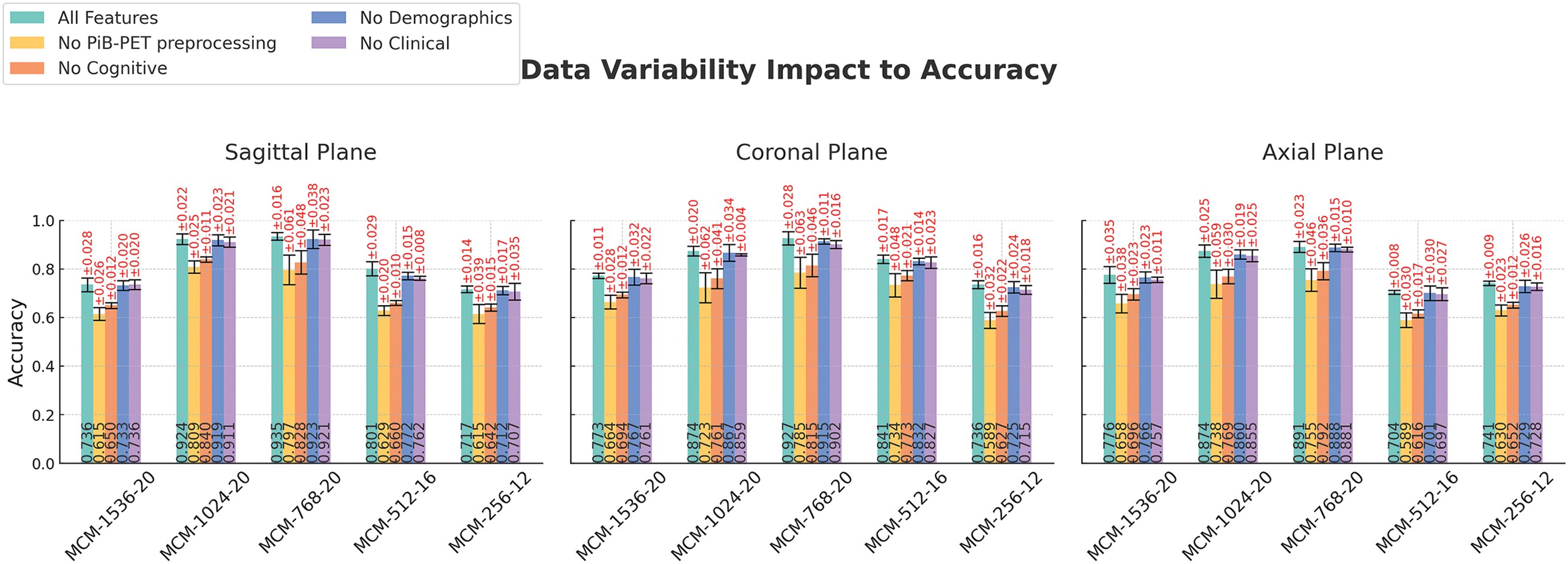
Figure 8: Feature category ablation studies across different imaging planes and models. Error bars are generated from 5 fold-cross validation results. Experiments performed on the full combined dataset (ADNI, MCSA, and OASIS3)

Models utilizing all features consistently achieve the highest accuracy across all planes, highlighting the importance of a dataset that contains more than one data modality. Removing cognitive test features (MMSE, CDR, and FAQ) results in the highest drop in accuracy (except for omitting motion correction and PVC in PiB-PET preprocessing), reinforcing their strong correlation with classification performance. This coincides with the feature correlation analysis depicted in Fig. 9.

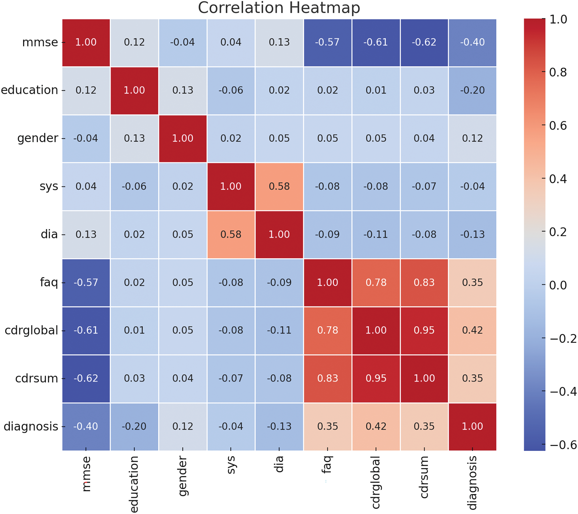
Figure 9: Correlation heatmap of numeric features. Cognitive tests (MMSE, FAQ, CDR-global and sum) have the highest correlation with diagnosis, where clinical parameters such as systolic and diastolic blood pressure, as well as demographic factors-education and gender, do not show a high correlation

The omission of demographic and clinical parameters also leads to reductions in accuracy, although relatively lower than the characteristics of cognitive tests. Variability in accuracy supports model stability, although MCM-1024 and MCM-768 produce notably higher performance than the baseline. A higher resilience to feature omission can be observed in the coronal plane, while the axial plane appears to be more sensitive to missing data, resulting in a slightly higher accuracy drop.

Removing PiB-PET preprocessing motion correction and PVC steps results in a consistent drop in accuracy across all models and planes. This highlights the importance of PiB-PET preprocessing for high classification performance. Higher cross-validation errors suggest increased variability and reduced model stability. This indicates that the absence of PiB-PET motion correction and PVC introduces more uncertainty in the classification results. These results highlight the need for cognitive features and PiB-PET preprocessing to achieve high classification accuracy.

To assess the generalizability of our models across different datasets, we performed Leave-One-Dataset-Out (LODO) cross-dataset validation. We compared its results with those achieved with 5-fold cross-validation and random split validation, which was reported in the main results section. For illustration purposes, we averaged the accuracies between planes and datasets. The comparison is represented in Fig. 10.

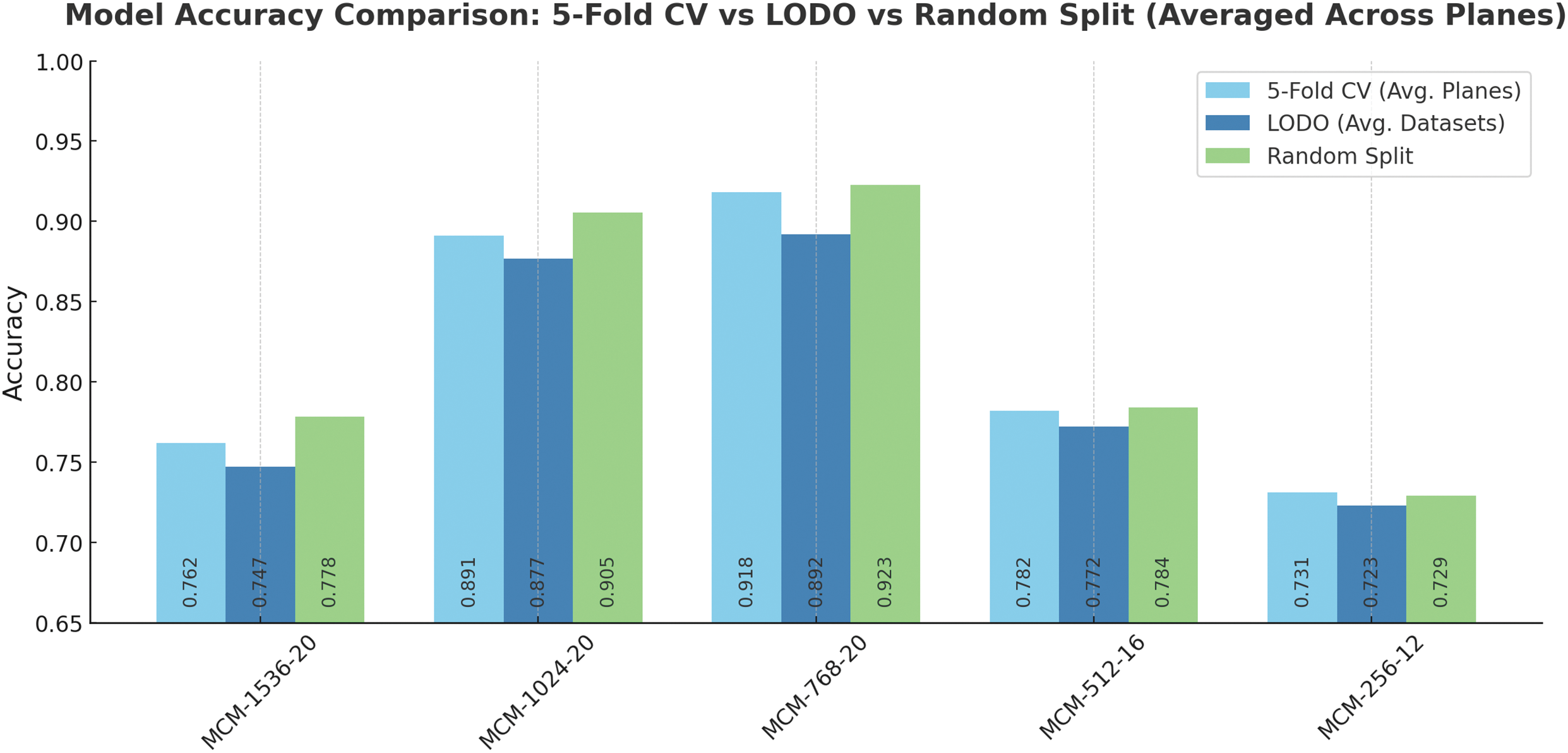
Figure 10: MCM models accuracy comparison using different validation methods (CV-5 fold cross-validation, LODO-Leave-One-Dataset-Out validation, and random train/validation dataset split). CV and random split were performed on the full dataset. Accuracies are averaged across planes and datasets for easier comparison

As shown in Fig. 10, 5-fold cross-validation yielded high overall accuracy, particularly for models with larger capacities such as MCM-768 and MCM-1024 (except for MCM-1536). These models consistently achieved accuracies above 89%, reflecting their ability to capture complex spatial features across imaging planes.

When evaluating the same models using the LODO validation strategy, accuracy remained comparable for MCM-768 and MCM-1024, suggesting strong cross-dataset generalization. In particular, LODO accuracy was slightly reduced for smaller models (MCM-512 and MCM-256), which may lack the representational capacity to adapt to shifts in data distributions between sources such as ADNI, MCSA, and OASIS3, indicating that while lightweight architectures, robustness may be compromised when encountering unseen data from different datasets.

Random train/validation split produced accuracy values comparable to or higher than 5-fold CV and LODO in several cases. This approach may overestimate model performance, as random split may not account for dataset-specific variability. Consequently, these results may not fully reflect real-world deployment scenarios, where models are expected to operate on previously unseen distributions. However, differences in the metric values are minimal (up to 3%), which highlights the robustness of the models given different subsets of the subjects of the dataset and other variations of the datasets, particularly variants MCM-1024 and MCM-768.

5  Discussion

In recent years, Multi-Layer Perceptron (MLP) mixers have gained attention due to their ability to match state-of-the-art performance while being more computationally efficient in parameters and computations [60,61]. ConvMixer adopts a similar approach, but instead of stacking dense layers, it employs convolutional layers, which can capture more spatially aware features from the data. One of the reasons we chose ConvMixer is its architectural simplicity. With only one layer type, the model is easy to extend and modify by adding new modules as needed. This modularity allows future improvements or adaptations in different domains or datasets.

Another important aspect of our work is the incorporation of Explainable Artificial Intelligence (XAI), which has become a rapidly growing area of interest in the AI research community. Traditionally, deep learning models have been considered “black boxes”, making them difficult to understand as to how they make decisions or what factors influence their predictions. However, advanced XAI methods are emerging that allow for a more straightforward interpretation of model decision-making. In our model, we used B-cos network modules to visually represent feature contributions as images are processed through the network. Unlike Grad-CAM, which produces only heatmaps, B-cos offers a more visually appealing and informative explanation of the decision-making process. B-cos has also been shown to improve metrics such as localization [44] compared to Grad-CAM, suggesting that it can provide more accurate insights into the areas of the input data that are most relevant for classification. Incorporating XAI into classification models will be crucial in the future, not just to create clearer visualizations of model decisions but also to improve the trust of practitioners in these methods, particularly when used in clinical settings.

One of the limitations of the study is the lack of validation in a real-world clinical setting. Although the study demonstrates promising classification performance with three publicly available datasets (ADNI, OASIS3, and MCSA), translating these findings into routine clinical practice presents several challenges. In real-world settings, variations in scanner hardware and imaging protocols can lead to differences in image quality and signal characteristics for T1w MRI and PiB-PET, potentially affecting the reliability of the neuroimaging input data. In addition, clinical workflows across institutions often vary, influencing how and when imaging, clinical, and demographic data are acquired and integrated. To ensure robust performance in diverse patient populations, it is recommended that the model be validated on a wider spectrum of studies, imaging environments, setups, and clinical practices.

For future work, an essential avenue for exploration is to conduct additional ablation studies to assess each data modality’s impact on the model’s performance. Although multimodal methods generally outperform single-modal approaches by using complementary information from different sources, it would be valuable to evaluate the individual contribution of each modality, whether imaging, clinical or demographic data, to overall model effectiveness. Understanding the relative importance of each modality could help refine the model and highlight which characteristics are most influential in distinguishing between patients with MCI and patients with Cognitively Normal (CN). We aim to improve the balance between sensitivity and specificity. In some instances, the model exhibited a trade-off, where one metric was higher than the other, leading to either more false positives or false negatives. Ideally, the balance between sensitivity and specificity should be minimal, meaning the model is confident in its decisions without sacrificing performance. Achieving this balance will improve the model’s reliability and make it suitable for practical use in clinical environments. As part of future improvements, we also plan to explore additional data modalities and techniques, such as incorporating T2w or Computed Tomography (CT), which may further improve the detection of MCI. Integrating such data could help improve the model’s predictive capabilities and increase its robustness when applied in a variety of real-world clinical contexts. The ongoing refinement of explainability methods and the fine-tuning of the model’s sensitivity and specificity could make it a valuable tool for early and accurate detection of MCI.

6  Conclusions

This study proposed a method for accurately detecting MCI using multimodal data. The combination of T1-weighted and PiB-PET brain imaging modalities provides valuable information on the structural and metabolic aspects of the brain, which are beneficial when detecting pathologies associated with MCI. In addition, the inclusion of cognitive test results, along with demographic and clinical data such as blood pressure parameters, education, and gender, contributes essential information that can offer a more comprehensive understanding of an individual’s cognitive status, as well as variations and clinical conditions that can influence the progression of MCI.

The proposed methodology integrates advanced deep learning techniques, utilizing a fusion of imaging modalities and a novel Multimodal Convolution Mixer architecture. This approach improves the accuracy, sensitivity, and specificity of MCI detection compared to traditional baseline models and provides visualizations of the most influential features in decision-making, thus improving interpretability. Using a custom classifier, combined with regularization strategies, further strengthens the robustness of the model against overfitting, enabling it to generalize across individual and mixed datasets effectively.

The ablation study identified the multi-head self-attention module as a pivotal component for improving model performance. In specific cases, this module facilitated a performance boost of 10%–20%, underscoring its critical role in the success of the model. These results highlight the potential for developing more accurate and reliable models for the detection of MCI, offering a promising avenue for future research. Using a multimodal approach and focusing on key neural mechanisms, this study sets the stage for further refinement of the MCI detection techniques. This could eventually lead to better diagnostic tools and personalized treatment options.

Acknowledgement: Not applicable.

Funding Statement: This research received no external funding.

Author Contributions: Conceptualization, Rytis Maskeliūnas; Data curation, Robertas Damaševičius; Formal analysis, Ovidijus Grigas, Robertas Damaševičius and Rytis Maskeliūnas; Funding acquisition, Rytis Maskeliūnas; Investigation, Ovidijus Grigas, Robertas Damaševičiuss and Rytis Maskeliūnas; Methodology, Ovidijus Grigas and Rytis Maskeliūnas; Project administration, Rytis Maskeliūnas; Resources, Ovidijus Grigas; Software, Ovidijus Grigas; Supervision, Rytis Maskeliūnas; Validation, Ovidijus Grigas and Robertas Damaševičius; Visualization, Ovidijus Grigas; Writing—original draft, Ovidijus Grigas; Writing—review & editing, Ovidijus Grigas and Rytis Maskeliūnas. All authors reviewed the results and approved the final version of the manuscript.

Availability of Data and Materials: The study used the following datasets:

•   Alzheimer’s Disease Neuroimaging Initiative (ADNI) (https://adni.loni.usc.edu/, accessed on 21 April 2025),

•   Mayo Clinic Study of Aging (MCSA) (https://www.mayo.edu/research/centers-programs/alzheimers-disease-research-center/research-activities/mayo-clinic-study-aging/overview, accessed on 21 April 2025),

•   Open Access Series of Imaging Studies (OASIS) (https://sites.wustl.edu/oasisbrains/home/oasis-3/, accessed on 21 April 2025).

Ethics Approval: Not applicable.

Conflicts of Interest: The authors declare no conflicts of interest to report regarding the present study.

References

1. Gauthier S, Reisberg B, Zaudig M, Petersen RC, Ritchie K, Broich K, et al. Mild cognitive impairment. The Lancet. 2006;367(9518):1262–70. doi:10.1016/S0140-6736(06)68542-5. [Google Scholar] [PubMed] [CrossRef]

2. Chan ATC, Ip RTF, Tran JYS, Chan JYC, Tsoi KKF. Computerized cognitive training for memory functions in mild cognitive impairment or dementia: a systematic review and meta-analysis. npj Digit Med. 2024;7(1):1. doi:10.1038/s41746-023-00987-5. [Google Scholar] [PubMed] [CrossRef]

3. Leon MJ, Mosconi L, Li J, De Santi S, Yao Y, Tsui WH, et al. Longitudinal CSF isoprostane and MRI atrophy in the progression to AD. J Neurol. 2007;254(12):1666–75. doi:10.1007/s00415-007-0610-z. [Google Scholar] [PubMed] [CrossRef]

4. Rangaraju B, Chinnadurai T, Natarajan S, Raja V. Dual attention aware octave convolution network for early-stage alzheimer’s disease detection. Inf Technol Control. 2024;53(1):302–16. doi:10.5755/j01.itc.53.1.34536. [Google Scholar] [CrossRef]

5. Karthigeyan CMT, Rani C. Optimizing parkinson’s disease diagnosis with multimodal data fusion techniques. Inf Technol Control. 2024;53(1):262–79. doi:10.5755/j01.itc.53.1.34718. [Google Scholar] [CrossRef]

6. Jack CR, Knopman DS, Jagust WJ, Shaw LM, Aisen PS, Weiner MW, et al. Hypothetical model of dynamic biomarkers of the Alzheimer’s pathological cascade. Lancet Neurol. 2010;9(1):119–28. doi:10.1016/S1474-4422(09)70299-6. [Google Scholar] [PubMed] [CrossRef]

7. Yin C, Li S, Zhao W, Feng J. Brain imaging of mild cognitive impairment and Alzheimer’s disease. Neural Regen Res. 2013 Feb;8(5):435–44. doi:10.3969/j.issn.1673-5374.2013.05.007. [Google Scholar] [PubMed] [CrossRef]

8. Grässler B, Herold F, Dordevic M, Gujar TA, Darius S, Böckelmann I, et al. Multimodal measurement approach to identify individuals with mild cognitive impairment: study protocol for a cross-sectional trial. BMJ Open. 2021;11(5):e046879. doi:10.1136/bmjopen-2020-046879. [Google Scholar] [PubMed] [CrossRef]

9. Kim SK, Duong QA, Gahm JK. Multimodal 3D deep learning for early diagnosis of alzheimer’s disease. IEEE Access. 2024;12(1):46278–89. doi:10.1109/ACCESS.2024.3381862. [Google Scholar] [CrossRef]

10. Zhang M, Sun L, Kong Z, Zhu W, Yi Y, Yan F. Pyramid-attentive GAN for multimodal brain image complementation in Alzheimer’s disease classification. Biomed Signal Process Control. 2024 Mar;89(1):105652. doi:10.1016/j.bspc.2023.105652. [Google Scholar] [CrossRef]

11. Kitajima K, Abe K, Takeda M, Yoshikawa H, Ohigashi M, Osugi K, et al. Clinical impact of 11C-Pittsburgh compound-B positron emission tomography in addition to magnetic resonance imaging and single-photon emission computed tomography on diagnosis of mild cognitive impairment to Alzheimer’s disease. Medicine. 2021 Jan;100(3):e23969. doi:10.1097/MD.0000000000023969. [Google Scholar] [PubMed] [CrossRef]

12. Buch VH, Ahmed I, Maruthappu M. Artificial intelligence in medicine: current trends and future possibilities. Br J Gen Pract. 2018;68(668):143–4. doi:10.3399/bjgp18X695213. [Google Scholar] [PubMed] [CrossRef]

13. Zhang ZC, Zhao X, Dong G, Zhao XM. Improving alzheimer’s disease diagnosis with multi-modal PET embedding features by a 3D multi-task MLP-mixer neural network. IEEE J Biomed Health Inform. 2023;27(8):4040–51. doi:10.1109/JBHI.2023.3280823. [Google Scholar] [PubMed] [CrossRef]

14. Di Benedetto M, Carrara F, Tafuri B, Nigro S, De Blasi R, Falchi F, et al. Deep networks for behavioral variant frontotemporal dementia identification from multiple acquisition sources. Comput Biol Med. 2022;148(1–2):105937. doi:10.1016/j.compbiomed.2022.105937. [Google Scholar] [PubMed] [CrossRef]

15. Zhou Z, Islam MT, Xing L. Multibranch CNN with MLP-mixer-based feature exploration for high-performance disease diagnosis. IEEE Trans Neural Netw Learn Syst. 2024;35(6):7351–62. doi:10.1109/TNNLS.2023.3250490. [Google Scholar] [PubMed] [CrossRef]

16. Trockman A, Kolter JZ. Patches are all you need? arXiv:2201.09792. 2022. [Google Scholar]

17. Hamet P, Tremblay J. Artificial intelligence in medicine. Metabolism. 2017;69(3):S36–40. doi:10.1016/j.metabol.2017.01.011. [Google Scholar] [PubMed] [CrossRef]

18. Holzinger A, Langs G, Denk H, Zatloukal K, Müller H. Causability and explainability of artificial intelligence in medicine. Wiley Interdiscip Rev Data Min Knowl Discov. 2019;9(4):e1312. doi:10.1002/widm.1312. [Google Scholar] [PubMed] [CrossRef]

19. Subramanyam Rallabandi VP, Seetharaman K. Deep learning-based classification of healthy aging controls, mild cognitive impairment and Alzheimer’s disease using fusion of MRI-PET imaging. Biomed Signal Process Control. 2023;80(8):104312. doi:10.1016/j.bspc.2022.104312. [Google Scholar] [CrossRef]

20. Forouzannezhad P, Abbaspour A, Li C, Fang C, Williams U, Cabrerizo M, et al. A Gaussian-based model for early detection of mild cognitive impairment using multimodal neuroimaging. J Neurosci Methods. 2020;333:108544. doi:10.1016/j.jneumeth.2019.108544. [Google Scholar] [PubMed] [CrossRef]

21. Perez-Gonzalez J, Jiménez-Ángeles L, Rojas Saavedra K, Barbará Morales E, Medina-Bañuelos V. Mild cognitive impairment classification using combined structural and diffusion imaging biomarkers. Phys Med Biol. 2021;66(15):155010. doi:10.1088/1361-6560/ac0e77. [Google Scholar] [PubMed] [CrossRef]

22. Kang L, Jiang J, Huang J, Zhang T. Identifying early mild cognitive impairment by multi-modality MRI-based deep learning. Front Aging Neurosci. 2020;12:206. doi:10.3389/fnagi.2020.00206. [Google Scholar] [PubMed] [CrossRef]

23. Chen H, Guo H, Xing L, Chen D, Yuan T, Zhang Y, et al. Multimodal predictive classification of Alzheimer’s disease based on attention-combined fusion network: integrated neuroimaging modalities and medical examination data. IET Image Process. 2023;17(11):3153–64. doi:10.1049/ipr2.12841. [Google Scholar] [CrossRef]

24. Dwivedi S, Goel T, Tanveer M, Murugan R, Sharma R. Multimodal fusion-based deep learning network for effective diagnosis of alzheimer’s disease. IEEE Multimed. 2022;29(2):45–55. doi:10.1109/MMUL.2022.3156471. [Google Scholar] [CrossRef]

25. Odusami M, Maskeliūnas R, Damaševičius R. Pareto optimized adaptive learning with transposed convolution for image fusion alzheimer’s disease classification. Brain Sci. 2023;13(7):1045. doi:10.3390/brainsci13071045. [Google Scholar] [PubMed] [CrossRef]

26. Odusami M, Damasevicius R, Milieskaite-Belousoviene E, Maskeliunas R. Multimodal neuroimaging fusion for alzheimer’s disease: an image colorization approach with mobile vision transformer. Int J Imaging Syst Technol. 2024;34(5):e23158. doi:10.1002/ima.23158. [Google Scholar] [CrossRef]

27. Grigas O, Damaševičius R, Maskeliūnas R. Positive effect of super-resolved structural magnetic resonance imaging for mild cognitive impairment detection. Brain Sci. 2024;14(4):381. doi:10.3390/brainsci14040381. [Google Scholar] [PubMed] [CrossRef]

28. Odusami M, Maskeliūnas R, Damaševičius R. Optimized convolutional fusion for multimodal neuroimaging in alzheimer’s disease diagnosis: enhancing data integration and feature extraction. J Pers Med. 2023;13(10):1496. doi:10.3390/jpm13101496. [Google Scholar] [PubMed] [CrossRef]

29. Odusami M, Damaševičius R, Milieškaitė-Belousovienė E, Maskeliūnas R. Alzheimer’s disease stage recognition from MRI and PET imaging data using Pareto-optimal quantum dynamic optimization. Heliyon. 2024;10(15):e34402. doi:10.1016/j.heliyon.2024.e34402. [Google Scholar] [PubMed] [CrossRef]

30. Ávila Villanueva M, Marcos Dolado A, Gómez-Ramírez J, Fernández-Blázquez M. Brain structural and functional changes in cognitive impairment due to alzheimer’s disease. Front Psychol. 2022;13:886619. doi:10.3389/fpsyg.2022.886619. [Google Scholar] [PubMed] [CrossRef]

31. Reitz C, Tang MX, Manly J, Mayeux R, Luchsinger JA. Hypertension and the risk of mild cognitive impairment. Arch Neurol. 2007;64(12):1734. doi:10.1001/archneur.64.12.1734. [Google Scholar] [PubMed] [CrossRef]

32. Gaussoin SA, Pajewski NM, Chelune G, Cleveland ML, Crowe MG, Launer LJ, et al. Effect of intensive blood pressure control on subtypes of mild cognitive impairment and risk of progression from SPRINT study. J Am Geriatr Soc. 2021;70(5):1384–93. doi:10.1111/jgs.17583. [Google Scholar] [PubMed] [CrossRef]

33. Mueller SG, Weiner MW, Thal LJ, Petersen RC, Jack CR, Jagust W, et al. Ways toward an early diagnosis in Alzheimer’s disease: the Alzheimer’s Disease Neuroimaging Initiative (ADNI). Alzheimer’s Dementia. 2005;1(1):55–66. doi:10.1016/j.jalz.2005.06.003. [Google Scholar] [PubMed] [CrossRef]

34. Mayo Clinic. Alzheimer’s Disease Research Center. [cited 2024 Dec 8]. Available from: https://www.mayo.edu/research/centers-programs/alzheimers-disease-research-center/research-activities/mayo-clinic-study-aging/overview. [Google Scholar]

35. LaMontagne PJ, Benzinger TL, Morris JC, Keefe S, Hornbeck R, Xiong C, et al. OASIS-3: longitudinal neuroimaging, clinical, and cognitive dataset for normal aging and alzheimer disease. 2019. doi:10.1101/2019.12.13.19014902. [Google Scholar] [CrossRef]

36. Smith SM, Jenkinson M, Woolrich MW, Beckmann CF, Behrens TEJ, Johansen-Berg H, et al. Advances in functional and structural MR image analysis and implementation as FSL. NeuroImage. 2004;23(5):S208–19. doi:10.1016/j.neuroimage.2004.07.051. [Google Scholar] [PubMed] [CrossRef]

37. Andrew Hoopes ZK Alexander Zsikla. Freesurfer: Neuroimaging Analysis and Visualization Suite. [cited 2024 Dec 8]. Available from: https://github.com/freesurfer/freesurfer. [Google Scholar]

38. Hoopes A, Mora JS, Dalca AV, Fischl B, Hoffmann M. SynthStrip: skull-stripping for any brain image. NeuroImage. 2022;260(1):119474. doi:10.1016/j.neuroimage.2022.119474. [Google Scholar] [PubMed] [CrossRef]

39. Greve DN, Svarer C, Fisher PM, Feng L, Hansen AE, Baare W, et al. Cortical surface-based analysis reduces bias and variance in kinetic modeling of brain PET data. NeuroImage. 2014;92(21):225–36. doi:10.1016/j.neuroimage.2013.12.021. [Google Scholar] [PubMed] [CrossRef]

40. Greve DN, Salat DH, Bowen SL, Izquierdo-Garcia D, Schultz AP, Catana C, et al. Different partial volume correction methods lead to different conclusions: an 18F-FDG-PET study of aging. NeuroImage. 2016;132:334–43. doi:10.1016/j.neuroimage.2016.02.042. [Google Scholar] [PubMed] [CrossRef]

41. Meechai T, Tepmongkol S, Pluempitiwiriyawej C. Partial-volume effect correction in positron emission tomography brain scan image using super-resolution image reconstruction. British J Radiol. 2015;88(1046):20140119. doi:10.1259/bjr.20140119. [Google Scholar] [PubMed] [CrossRef]

42. Yildirim N. Deep image fusion: multi-sensor image (infrared and visible) Fusion using deep learning framework, Principal Component Analysis, Discrete Wavelet Transform—github.com. [cited 2024 Dec 27]. Available from: https://github.com/nuriyeyldrm/deep_image_fusion. [Google Scholar]

43. Hendrycks D, Gimpel K. Gaussian error linear units (GELUs). arXiv:1606.08415. 2016. [Google Scholar]

44. Böhle M, Singh N, Fritz M, Schiele B. B-Cos alignment for inherently interpretable CNNs and vision transformers. IEEE Trans Pattern Anal Mach Intell. 2024;46(6):4504–18. doi:10.1109/TPAMI.2024.3355155. [Google Scholar] [PubMed] [CrossRef]

45. Chollet F. Xception: deep learning with depthwise separable convolutions. In: 2017 IEEE Conference on Computer Vision and Pattern Recognition (CVPR). IEEE; 2017 Jul. p. 1800–7. doi:10.1109/cvpr.2017.195. [Google Scholar] [CrossRef]

46. Dosovitskiy A, Beyer L, Kolesnikov A, Weissenborn D, Zhai XH, Unterthiner T, et al. An image is worth 16 × 16 words: transformers for image recognition at scale. arXiv:2010.11929. 2020. [Google Scholar]

47. Pan X, Ye T, Xia Z, Song S, Huang G. Slide-transformer: hierarchical vision transformer with local self-attention. In: 2023 IEEE/CVF Conference on Computer Vision and Pattern Recognition (CVPR). IEEE; 2023 Jun. p. 2082–91. doi:10.1109/CVPR52729.2023.00207. [Google Scholar] [CrossRef]

48. Leem S, Seo H. Attention guided CAM: visual explanations of vision transformer guided by self-attention. arXiv:2402.04563. 2024. [Google Scholar]

49. Selvaraju RR, Cogswell M, Das A, Vedantam R, Parikh D, Batra D. Grad-CAM: visual explanations from deep networks via gradient-based localization. Int J Comput Vis. 2019;128(2):336–59. doi:10.1007/s11263-019-01228-7. [Google Scholar] [CrossRef]

50. Lundberg S, Lee SI. A unified approach to interpreting model predictions. arXiv:1705.07874. 2017. [Google Scholar]

51. Vaswani A, Shazeer N, Parmar N, Uszkoreit J, Jones L, Gomez AN, et al. Attention is all you need. arXiv:1706.03762. 2017. [Google Scholar]

52. He K, Zhang X, Ren S, Sun J. Deep residual learning for image recognition. arXiv:1512.03385. 2015. [Google Scholar]

53. Huang G, Liu Z, van der Maaten L, Weinberger KQ. Densely connected convolutional networks. arXiv:1608.06993. 2016. [Google Scholar]

54. Qin D, Leichner C, Delakis M, Fornoni M, Luo S, Yang F, et al. MobileNetV4: universal models for the mobile ecosystem. arXiv:2404.10518. 2024. [Google Scholar]

55. Smith EE, Egorova S, Blacker D, Killiany RJ, Muzikansky A, Dickerson BC, et al. Magnetic resonance imaging white matter hyperintensities and brain volume in the prediction of mild cognitive impairment and dementia. Arch Neurol. 2008;65(1). doi:10.1001/archneurol.2007.23. [Google Scholar] [PubMed] [CrossRef]

56. Solé-Padullés C, Bartrés-Faz D, Junqué C, Vendrell P, Rami L, Clemente IC, et al. Brain structure and function related to cognitive reserve variables in normal aging, mild cognitive impairment and Alzheimer’s disease. Neurobiol Aging. 2009;30(7):1114–24. doi:10.1016/j.neurobiolaging.2007.10.008. [Google Scholar] [PubMed] [CrossRef]

57. Zhang Y, Schuff N, Camacho M, Chao LL, Fletcher TP, Yaffe K, et al. MRI markers for mild cognitive impairment: comparisons between white matter integrity and gray matter volume measurements. PLoS One. 2013;8(6):e66367. doi:10.1371/journal.pone.0066367. [Google Scholar] [PubMed] [CrossRef]

58. Raine PJ, Rao H. Volume, density, and thickness brain abnormalities in mild cognitive impairment: an ALE meta-analysis controlling for age and education. Brain Imaging Behav. 2022;16(5):2335–52. doi:10.1007/s11682-022-00659-0. [Google Scholar] [PubMed] [CrossRef]

59. van der Meer D, Kaufmann T. Mapping the genetic architecture of cortical morphology through neuroimaging: progress and perspectives. Transl Psychiatry. 2022;12(1):447. doi:10.1038/s41398-022-02193-5. [Google Scholar] [PubMed] [CrossRef]

60. Tolstikhin I, Houlsby N, Kolesnikov A, Beyer L, Zhai XH, Unterthiner T, et al. MLP-Mixer: an all-MLP architecture for vision. arXiv:2105.01601. 2021. [Google Scholar]

61. Zhang H, Dong Z, Li B, He S. Multi-Scale MLP-Mixer for image classification. Knowl Based Syst. 2022;258(5):109792. doi:10.1016/j.knosys.2022.109792. [Google Scholar] [CrossRef]