Short-Term Electricity Load Forecasting Based on T-CFSFDP Clustering and Stacking-BiGRU-CBAM

1  Introduction

Power load forecasting is mainly based on historical data to predict future load demand [1]. The accuracy of prediction has become a key indicator for measuring the modernization level of power enterprise management, and it is also an important foundation for achieving modernization and scientific management of the power grid [2]. Power load forecasting is classified into long-term, medium-term, short-term, and ultra-short-term categories based on varying time scales. Among them, short-term load forecasting concentrates on predicting daily or weekly electricity consumption demands and is vital for the efficient operation and dispatch of power systems. Therefore, load forecasting has become an indispensable task within the framework of the power system from the point of view of guaranteeing security, improving economic efficiency and promoting long-term development [3].

Traditional forecasting methods, like trend extrapolation [4], regression analysis [5], and time series analysis [6], rely mainly on historical load data. These methods work well for data with minimal trend changes but suffer a sharp drop in prediction accuracy when trends change significantly. With deep-learning’s growth, many scholars worldwide have delved into short-term load forecasting, introducing effective models. Recurrent Neural Network (RNN)-based neural networks are prominent in load forecasting [7]. But RNNs face issues like gradient vanishing and explosion. To address this, Gated Recurrent Unit (GRU) was proposed by adding update and reset gates to traditional RNNs, offering a clear upgrade over RNNs and older machine-learning methods [8]. In load forecasting, while GRU-based models are somewhat widely used, they can’t capture data’s bidirectional dependency, leading to subpar forecasts. To let GRUs learn bidirectional temporal features, Bi-directional Gated Recurrent Unit (BiGRU) was developed as an extension of unidirectional GRUs. By combining forward and backward GRUs, BiGRU comprehensively captures bidirectional dependencies in time-series data, outperforming GRU in prediction [9].

Load data has a certain periodicity, and the widespread integration of new energy microgrids further intensifies this periodicity. As a result, relying solely on a single model or method rarely achieves the desired prediction effect. Previous research has explored diverse methods. Reference [10] proposes a multivariate real-time rolling decomposition paradigm, which achieves point and interval based power load forecasting by constructing a hybrid power load forecasting system. Reference [11] proposes a hybrid grey model that integrates multiple methods to reduce external interference. Optimize using an enhanced multi-objective slime mold algorithm to predict the trend of electricity consumption during the 15th Five Year Plan period. Reference [12] proposes an efficient interval prediction method that utilizes an innovative field mixer to mine spatiotemporal information, improves accuracy by utilizing adjacent field data, breaks the black box with interpretability analysis, and achieves accurate wind power prediction. Reference [13] uses the improved Northern Eagle optimization algorithm to optimize model parameters for power load forecasting, where the model integrates multiple components to leverage their strengths. Reference [14] constructs a load forecasting model using Convolutional Neural Network (CNN) and multilayer extended long short-term memory (LSTM) neural networks, where CNN extracts local features and LSTM captures long-term dependencies. Reference [15] uses an adaptive hierarchical clustering algorithm to filter input datasets for short-term electricity load forecasting, with a model based on the stacked integration of CNN-BiLSTM-Attention and XGBoost.

In summary, although modern short-term load forecasting (STLF) methods have seen some success, previous clustering algorithms can’t handle dynamic time-series data, and the simple fusion of forecasting models with classical attention mechanisms can’t meet current load forecasting needs and lacks innovation. This paper presents a new data-mining and deep-learning-based model. It innovatively improves the CFSFDP algorithm to handle dynamic data, enabling more effective time-series data clustering. Applying the Temporal-Clustering by Fast Search and Find of Density Peaks (T-CFSFDP) [16] to load curve clustering provides a more reliable data foundation for short-term load forecasting. The paper also breaks traditional boundaries by introducing the Convolutional Block Attention Module (CBAM) into load forecasting, significantly enhancing the model’s ability to recognize key temporal features [17]. A sub-model integration strategy for clustered data further boosts the model’s performance in capturing trends. The integration of the T-CFSFDP algorithm and the BiGRU-CBAM model is novel in the STLF field. Finally, five evaluation criteria validate the effectiveness of this integration technique, offering valuable insights for future load forecasting research.

The primary work conducted in this paper includes the following aspects:

(1) Optimize the clustering algorithm: The previous CFSFDP algorithm is not able to deal with temporal data well, by introducing the time decay factor, it makes it able to better take into account the temporal nature of the data, and the clustering effect of the time series is further improved.

(2) Applying convolutional block attention mechanism: CBAM was initially proposed to be used in the field of image recognition, but its application in load prediction is still relatively limited. In this paper, CBAM is combined with BiGRU to endow the model with the ability to pay attention to key data information, which significantly improves the prediction accuracy of the model.

(3) Stacking model stacking: Based on the clustering results of T-CFSFDP, the corresponding sub-models are trained separately for each category of data, and XGBoost is used as a meta-model to be integrated with stacking model stacking to form the final prediction model.

2  Introduction to Clustering Algorithms and Their Optimization

2.1 Peak Density Fast Search Algorithm

In 2014, Rodriguez and Laio proposed Clustering by Fast Search and Find of Density Peaks [18]. Unlike other density-based clustering algorithms, CFSFDP uses local density for fast and efficient sample point classification and outlier removal [19]. It doesn’t need pre-specifying the number of clusters or complex parameter settings, making it more user-friendly than many traditional clustering methods. This is crucial for short-term load forecasting data, as data distribution and the number of potential clusters are often unknown before forecasting. The algorithm is based on two assumptions: cluster centers are in highly-dense data areas, and their distance to other cluster centers is large relative to local data points. Thus, density and distance are key parameters in CFSFDP. For each data point x, the relevant formulas are calculated as follows:

{ρu=∑v=1,v≠iNexp(−guv2gk2)δu=minv:ρv>ρu(duv)(1)

where guv is the distance between data points u and v, gk is the cutoff distance, ρu is the local density of data point u, and δu is the minimum distance from point u to ρu a higher point.

2.2 Time-Series Weighted Density Peaks Clustering Algorithm

The CFSFDP algorithm, a machine-learning-based grouping method, has limitations in historical load data cluster analysis. When calculating the Euclidean distance between data points, it often misclassifies points with distinct peaks, resulting in inaccurate clustering. Moreover, since it ignores the time-series order of input data, it cannot handle time-series data well. Time-series changes don’t affect its final clustering results. Thus, the algorithm requires further optimization to fit the characteristics of time-series data better.

To address the density peak clustering algorithm’s neglect of data input temporal nature, this article enhances CFSFDP. It introduces time-dimension information and adds a time-weighting factor ti during topological-relationship calculation. The time weighting factor ti serves to weight and adjust the calculation of the distance between data points according to their timestamps. Specifically, for two data points xi and xj, the original Euclidean distance d(xi,xj) will be adjusted to d(xi,xj)=d(xi,xj)×ti×tj in calculating the distance between them, where ti and tj are the time weighting factors corresponding to data points xi and xj, respectively. ti’s value is usually based on the data points’ distance from the current time. The value of ti is usually determined according to the distance of the data point from the current time, the closer to the current time, the larger the value of ti, and vice versa, the smaller, thus strengthening the dynamic processing capability of time series data.

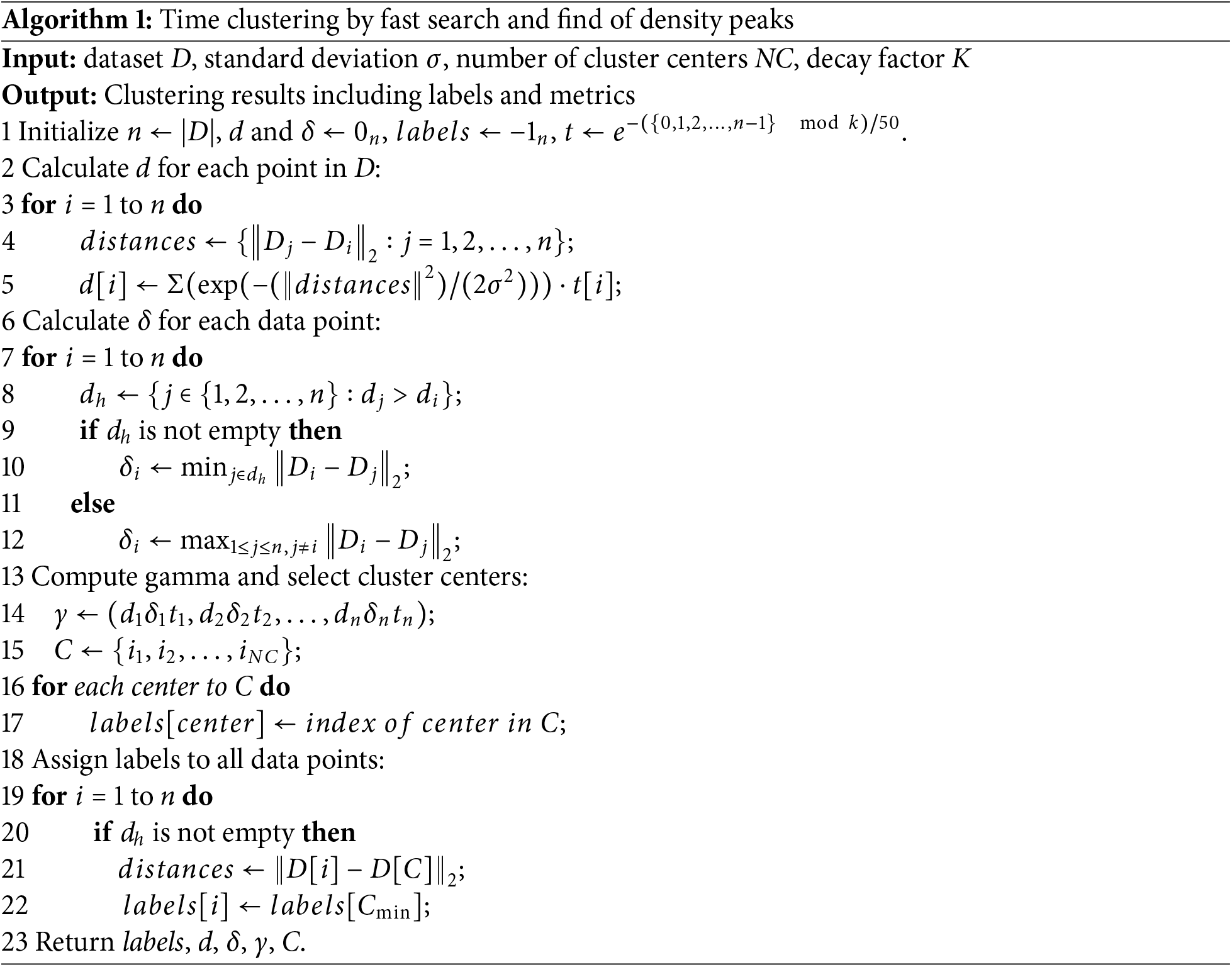
Through a large number of experiments, in order to prevent problems such as excessive computation or degradation of clustering quality due to improper setting of the time decay factor, it is determined that the optimal clustering performance can be achieved by setting the bandwidth of the time decay factor to 50, and the clustering accuracy is 0.6709. Its pseudocode is in Algorithm 1, and the specific process is illustrated in Fig. 1.

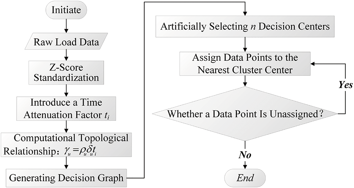
Figure 1: Flowchart for time-weighted density peak clustering

2.3 Clustering Performance Analysis

In this study, the two core parameters of the T-CFSFDP algorithm were set as follows: Gaussian kernel function standard deviation σ=1.5, and time span k=24. In order to accurately determine the number of cluster centers in the T-CFSFDP algorithm, a decision graph was drawn and the cluster centers were identified through manual observation. The decision diagram is shown in Fig. 2. In the upper right corner, there is a point with a high local density. Between [10000, 16000], there is a significant difference in decision values between the two points. The remaining data points are located in the lower right corner. Therefore, this article sets the number of cluster centers to 4 and assigns the remaining data points to these centers.

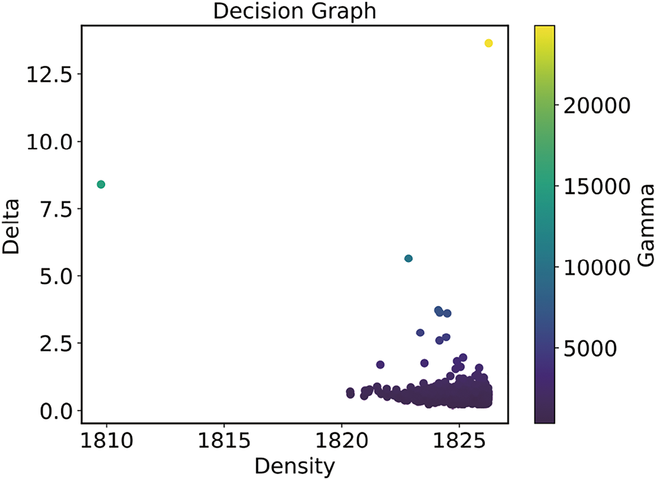
Figure 2: Decision-making maps produced by T-CFSFDP

After preprocessing the data, the original daily load profile samples were clustered using the T-CFSFDP clustering algorithm, and four classes of typical load profile samples were obtained. As shown in Fig. 3, the figure demonstrates these four classes of clustered load profile samples and the clustering over time, where the red dashed line is the center of each cluster.

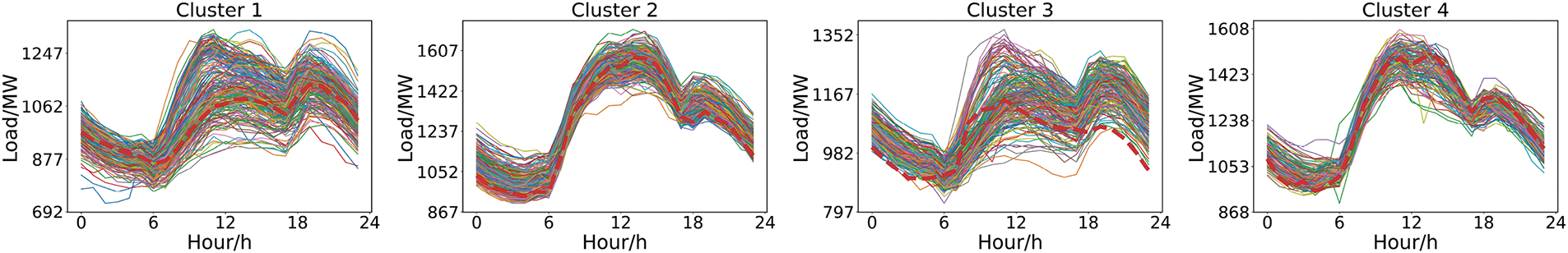
Figure 3: T-CFSFDP clusters load data into four categories

To verify the effectiveness of the clustering method in this paper, three metrics are used to evaluate the performance of clustering:

(1) Davies-Bouldin Index (DBI, Davidson-Bouldin Index) is a measure of the effectiveness of clustering, which reflects the quality of clustering by evaluating the compactness within clusters as well as the separation between clusters. The lower value of DBI means the better the clustering result. The formula of DBI is defined as follows:

DBI=1N∑i=1Nmaxj≠iFi¯+Fj¯‖wi−wj‖2(2)

where F¯i is the average Euclidean distance from the sample of class i to its class center, and ‖wi−wj‖2 is the class center Euclidean distance for classes i and j.

(2) Dunn’s Validity Index (DVI, Dunn’s Index) evaluates clustering quality. It’s derived from the ratio of intra-cluster closeness to inter-cluster distance. A higher DVI value indicates superior clustering. The formula for calculating DVI is as follows:

DVI=max1≤i≤k(mini≠jdinter,ijdintra,i)(3)

where d{inter},ij denotes the shortest distance between cluster i and cluster j, and d{intra},i is the maximum value of the distance from all points inside the ith cluster to the center of that cluster.

(3) Silhouette Coefficient (SC, Silhouette Index) is a measure of clustering effectiveness that evaluates the consistency of a data point with the cluster to which it belongs and its separation from other clusters. A higher value of SC implies that the data point belongs more to the current cluster and is more clearly delineated from the other clusters, thus reflecting a better clustering quality.

SC=1n∑i=1nu(xi)−v(xi)max{v(xi),u(xi)}(4)

where v(xi) denotes the average distance from xi to each data point in the same cluster and u(xi) denotes the average distance from xi to each data point in the closest cluster.

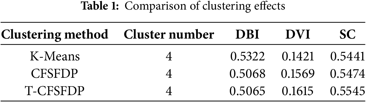
Compare the T-CFSFDP clustering algorithm with K-Means and CFSFDP clustering algorithms by calculating the values of the DBI, DVI, and SC metrics. The various indicators are presented in Table 1, and it can be seen that the T-CFSFDP algorithm achieved the best clustering performance.

3  Model Structure and Method Description

3.1 BiGRU Network

In unidirectional neural networks, information propagates in a sequential front-to-back manner. However, electricity load depends on both historical and future periods, and a single GRU neural network has difficulty fully extracting the deep features of relevant data [20]. To overcome the shortcoming of unidirectional information flow, this article uses the BiGRU model to improve the performance of power load forecasting [21]. Its specific details are shown in Fig. 4.

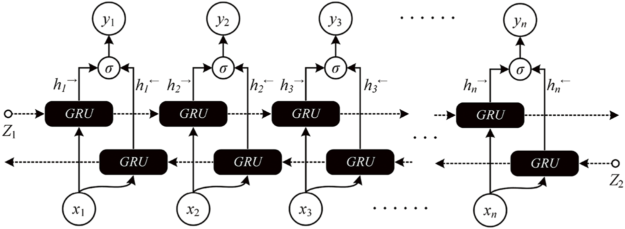
Figure 4: BiGRU network structure

Where Z1 and Z2 represent the initial positions of the two propagation directions, respectively. x1,x2,x3,…,xt denote the corresponding input timing signals at each moment, and y1,y2,y3,…,yt denote the corresponding outputs.

3.2 Convolutional Block Attention Mechanism

CBAM is an effective end-to-end attention mechanism. It contains two interconnected modules: channel attention and spatial attention. CBAM calculates weights for feature maps in the channel and spatial dimensions. After that, it multiplies these weights by the original feature maps, thereby adaptively strengthening features. When the CBAM module is integrated into the network, the network can better identify and use prominent features. This optimizes the overall performance of the model and significantly improves the accuracy of prediction tasks.

The CBAM network architecture is shown in Fig. 5. The channel attention module effectively filters important information from the input data, and the calculation formula is as follows:

Mc(F)=σ(MLP(AvgPool(F))+MLP(MaxPool(F)))=σ(W1(W0(Favgc))+W1(W0(Fmaxc)))(5)

where σ is the sigmoid function, W0∈RC/r×C and W1∈RC/r×C, and the MLP weights W0 and W1 are shared for both inputs.

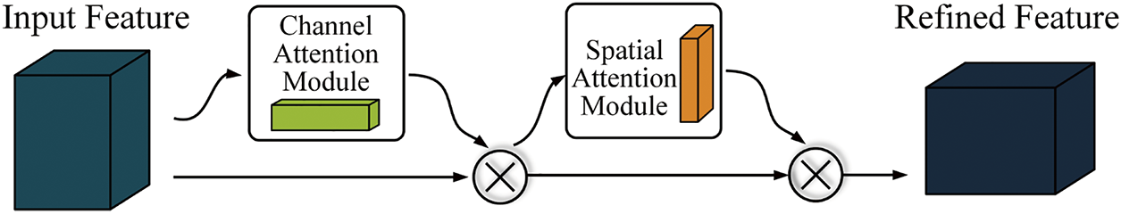
Figure 5: CBAM attention mechanism structure

The spatial attention module mainly focuses on which position information is meaningful, which is a supplement to channel attention. Its calculation formula is as follows:

Ms(F)=σ(f7×7([AvgPool(F),MaxPool(F)]))=σ(f7×7([Favgs,Fmaxs]))(6)

where a is the sigmoid function and f7×7 denotes the convolution operation with a filter size of 7×7.

3.3 Overall Process Description

This article proposes a T-CFSFDP algorithm and a stacked BiGRU-CBAM method for short-term power load forecasting. T-CFSFDP clustering preprocesses data to identify intrinsic clusters and provides structured input to the BiGRU-CBAM model, enabling it to more effectively handle datasets with complex temporal and feature correlations. The basic structural design is shown in the Fig. 6.

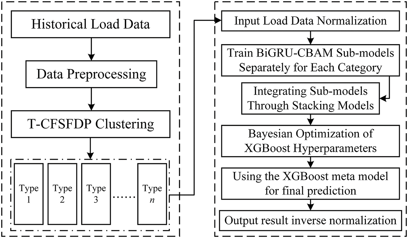
Figure 6: Flowchart of the prediction method based on T-CFSFDP clustering and BiGRU-CBAM models

(1) Data preprocessing: Due to power outages and equipment issues, the historical load time series dataset contains bias values and noise. In order to ensure reliable data for subsequent analysis, the original dataset was preprocessed. The preprocessing rules are as follows: replace outliers <400 with the average of adjacent values; When the adjacent values fluctuate greatly (| current – previous |>300), replace with the sum of the previous values. Moreover, to remove the impact of numerical units among different factors and simplify the training of network models, the original data is normalized to the interval of [0, 1]. Meanwhile, for the purpose of better aligning with the actual physical significance of the predicted outcomes and enabling easier comparison and analysis with the initial data, the predicted data undergoes inverse normalization. The calculation formulas for normalization and anti normalization are as follows:

{M′=M−MminMmax−MminA′=M′(Mmax−Mmin)+Mmin(7)

where M is the original load data, M′ and A′ are the normalized and denormalized load data, respectively, and Mmin and Mmax are the minimum and maximum values in the original load sequence, respectively.

(2) Cluster analysis: After clustering historical load data using T-CFSFDP, the cluster centers of the four clusters were determined to be 34441, 43417, 39457, and 37904, respectively. Subsequently, the data points are assigned to the corresponding clusters based on their proximity to these centroids.

(3) Model building: For each cluster, a BiGRU model with the CBAM module is trained. CBAM, composed of channel and spatial attention modules, adaptively adjusts feature maps. In the channel attention module, the global average and max pooling of input feature maps are done. The results are processed by MLP, summed, and Sigmoid-activated to get weights for channel adjustment. The spatial attention module averages and max-pools processed feature maps in the channel dimension and spliced them. They used convolution and Sigmoid to get weights for spatial adjustment and CBAM feature extraction. Then, CBAM-processed feature maps are input into BiGRU which processes sequence data from both directions to capture context and build the model.

(4) Integrated model prediction: For each cluster, the relevant sub-models are trained independently, using the mean square error as the loss function and the Adam optimizer to improve the training results. The training period is set to 120 times, the batch size is set to 64, and the number of GRU units is set to 64, too. The training set data is used for iterative training, and the model parameters are continuously fine-tuned to reduce the loss value to gradually achieve the best model performance. After the sub-model training is completed, the prediction results of the sub-models are collected by overlaying. The XGBoost meta-model parameters are automatically optimized by combining them with Bayesian optimization. Finally, the adjusted meta-model is used to complete the prediction.

4  Example Analysis and Performance Evaluation

4.1 Data Set Description and Evaluation Criteria

The dataset in this paper is taken from the literature [22], and all load data is obtained from the local grid operator in Panama. There are no missing values on the dataset, but only a few low values on the loads were detected, probably due to problems such as hourly outages and grid damage, in addition all records were kept. In this paper, the historical load data of which is selected from 4 January 2015, 00:00 to 4 January 2020, 23:00, a total of 5 years, the sampling interval of the data is 1 h, the cumulative load value between 00:00 and 01:00 is the first sampling data, and 24 points are collected every day, a total of 43,848 valid load data. The time-series data is sliced in the ratio of 3:1:1, the first 60% of the dataset is used as a training set to train the prediction model, and the last 40% is divided equally into validation set and test set.

In order to better analyze the research data, the load data from 2015 to 2020 were plotted as a load sample curve, as shown in Fig. 7. The green area in the figure represents the average load level, while the gray shaded area reflects the fluctuation range of the load. It can be seen that the changes in load are relatively periodic, and the fluctuations in peak and valley values indicate significant changes in power load within a certain time interval.

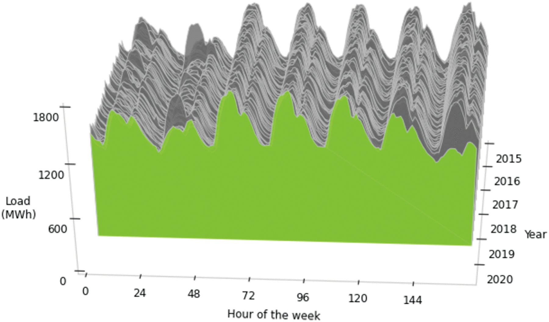
Figure 7: Trend chart of dataset load situation

This article selects seven evaluation metrics to assess predictive performance, namely MSE, MAE, MAPE, RMSE, and R2. The metric calculation formula is as follows:

{FMSE=1n∑i=1n(ki−k^i)2,FMAE=1n∑i=1n|k^i−ki|,FMAPE=100%n∑i=1n|k^i−kiki|FRMSE=1n∑i=1n(ki−k¯i)2,FR2=1−∑i=1n(k^i−ki)2∑i=1n(ki−1n∑i=1nki)2(8)

where k^i and ki are the predicted load value and load true data value of the ith load point in the test set, respectively; n is the number of prediction points.

4.2 Experimental Analysis and Model Evaluation

4.2.1 Analysis of Multidimensional Requirements for Model Implementation

In terms of hardware, the CPU needs to handle a large number of matrix operations, such as XGBoost training, T-CFSFDP function distance calculation, etc. To efficiently complete intensive numerical operations, it is recommended to use multi-core processors. For the bidirectional GRU layer computation of deep learning model training in sub models, a GPU that supports CUDA acceleration and has video memory should be equipped. In terms of memory, due to the need to store large amounts of data and intermediate results in the code, at least 16 GB of memory is required to ensure smooth operation. At the software level, Python 3.10, Keras 2.12, Xgboost 2.0.3, Pandas 1.4.3, Scikit-learn 1.4.1. post1, and NumPy 1.23.5 are used for data processing, model development, and evaluation.

In the comprehensive evaluation of the overall prediction process, this article first focuses on the running time of clustering algorithms. The T-CFSFDP algorithm takes 15.9433 s, slightly higher than the CFSFDP algorithm’s 15.6106 s. Due to the high time complexity of T-CFSFDP, its running time is significantly higher than traditional clustering methods such as DBSCAN (0.2034 s) and K-Means (0.1953 s). Secondly, in terms of model running time, BiGRU-CBAM takes 1259.35 ms per batch of training, which is longer than GRU’s 871.71 ms and LSTM’s 1199.87 ms, mainly due to its more complex structure.

In summary, the method proposed in this paper is longer than the conventional prediction method in terms of running time, although its prediction accuracy is significantly improved, which is a strategy of trading time for accuracy. Moreover, the additional increase in elapsed time is within the acceptable range.

4.2.2 Bayesian Optimization of XGBoost Hyperparameters

In this paper, model integration is achieved via the meta-model XGBoost, which utilizes the historical training information of each sub-model for final prediction. Thus, choosing a reasonable set of hyper-parameters is crucial for enhancing model accuracy. Therefore, the Bayesian optimization algorithm is adopted to optimize the model parameters. After 20 iterations of the Bayesian optimization algorithm, an optimal set of parameter combinations was determined. Specifically, the learning rate was set at 0.05, the maximum depth was 3.061, and the number of estimators was 106.5.

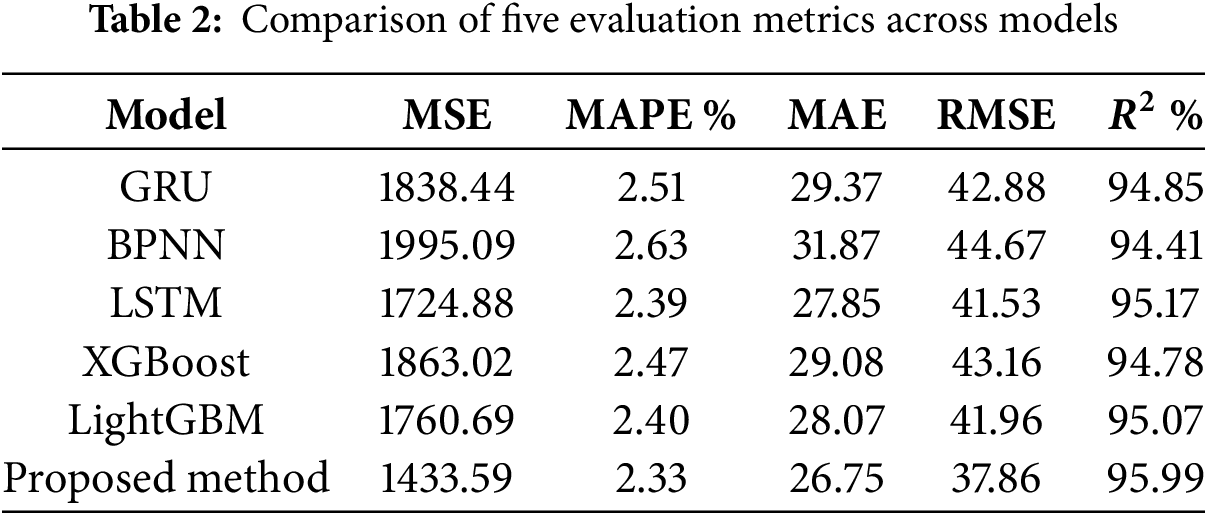
4.2.3 Comparison of Prediction Accuracy

In this article, we divide the dataset into small time periods with the aim of accurately predicting the load for the next 48 h. To verify the effectiveness of the proposed method, this paper compared GRU, BPNN, LSTM, XGBoost, and LightGBM. Meanwhile, in order to ensure the rigor of the experiment, the internal parameters of all models are kept consistent. As shown in Table 2, the proposed method shows the highest prediction accuracy under the five different evaluation criteria. Its MSE is only 1433.59, which is 21.967%, 28.127%, 16.927%, 22.986%, and 18.586% higher than the other models, and its MAPE is only 2.33%, which is 7.171%, 11.403%, 2.511%, 5.672%, and 2.917% higher than the five counterpart models. Its MAE is 26.75, which is 8.924%, 16.084%, 3.949%, 7.996%, and 4.703% higher than the five corresponding models, and its RMSE is 11.713%, 15.209%, 8.845%, 12.279%, and 9.752% higher than the five corresponding models. The RMSE is 11.713%, 15.209%, 8.845%, 12.279% and 9.713%, respectively. Under the R2 criterion, it is 1.14%, 1.58%, 0.82%, 1.21% and 0.92% better than the other prediction models, respectively.

To further illustrate the advantages of our proposed model in short-term power load forecasting, we compared our method with the GRU-CNN model in reference [23] and the CNN-GRU-Attention prediction model in reference [24]. As shown in Fig. 8, our proposed method has the highest prediction accuracy under three different evaluation indicators, with RMSE improving by about 10.31% and 7.91%, MAE improving by about 4.16% and 4.40%, R2 improving by about 2.14% and 1.74%, and MAPE improving by only 2.33%, compared to the other two models by 4.12% and 4.90%, respectively.

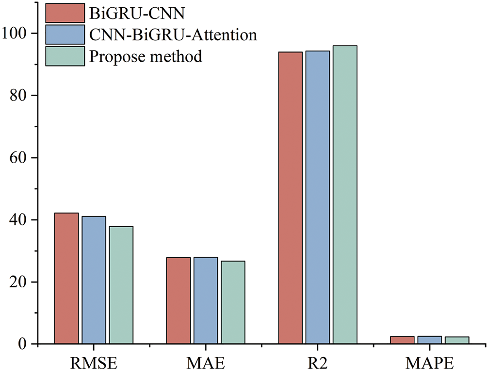
Figure 8: Comparison of four types of evaluation metrics RMSE, MAE, R2, MAPE

To evaluate the generalization, stability, and robustness of the model, this paper uses cross validation to comprehensively examine its performance. The average MSE, RMSE, MAE, MAPE, and R2 values obtained from the cross validation experiment were 0.00049, 0.02195, 0.01577, 0.02400, and 0.93927, respectively. The results show that the model possesses a great degree of accuracy, good fitting effect, and reliable data prediction.

4.2.4 Ablation Experiment

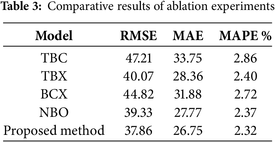
To verify the effectiveness of each component of the method proposed in this article, ablation experiments were conducted. Meanwhile, in order to ensure the validity of the experiment, only a portion of the entire method was deleted or modified, while the rest remained unchanged. The following is a description of the ablation experiment:

(1) T-CFSFDP+BiGRU-CBAM represents a processing method that does not use a meta model to integrate XGBoost models, but instead uses the conventional weighted average to integrate sub models. At the same time, for convenience, the name will be changed to TBC;

(2) T-CFSFDP+BiGRU+XGBoost indicates a method that does not introduce the CBAM attention mechanism. At the same time, to simplify the name changed to TBX;

(3) BiGRU-CBAM+XGBoost means that T-CFSFDP clustering is not used. Change it to BCX with the simplified name above;

(4) T-CFSFDP+BiGRU+NoBO represents an experiment that does not use Bayesian optimization, and is simplified and named NBO to highlight its characteristics.

From the comparative results of the ablation experiments in Table 3, it can be seen that under different evaluation indicators, the average RMSE improvement of the method proposed in this paper is about 11.66%, MAE is about 12.26%, and MAPE is about 10.34%, which proves the effectiveness of each module.

4.2.5 Model Performance Analysis

In this paper, we compare the load prediction curves of the proposed method with those of GRU, GRU-CNN, and CNN-GRU-Attention to visualize the higher agreement between their prediction curves and the actual load. As can be seen from Fig. 9a, the prediction performance of the baseline GRU model is inferior to that of this paper’s method during periods of high power load fluctuations. From Fig. 9b, the introduction of convolutional neural network improves the smoothness of the prediction curve. Compared with unidirectional GRU, BiGRU is more capable of capturing the changing trend of load data, which also makes the prediction effect of this paper’s method better. Fig. 9c shows that the combined model containing the attention mechanism has high prediction accuracy in the region of sharp fluctuations, but in the interval where the load is relatively smooth but has a weak trend change, the prediction error accumulates because the attention mechanism pays too much attention to the significant fluctuations and ignores the potential trend in the smooth section. In contrast, the method in this paper presents stable and excellent prediction performance in all kinds of load change scenarios by virtue of its comprehensive and balanced feature extraction and analysis capabilities, which provides a more reliable solution for accurate load forecasting in power systems.

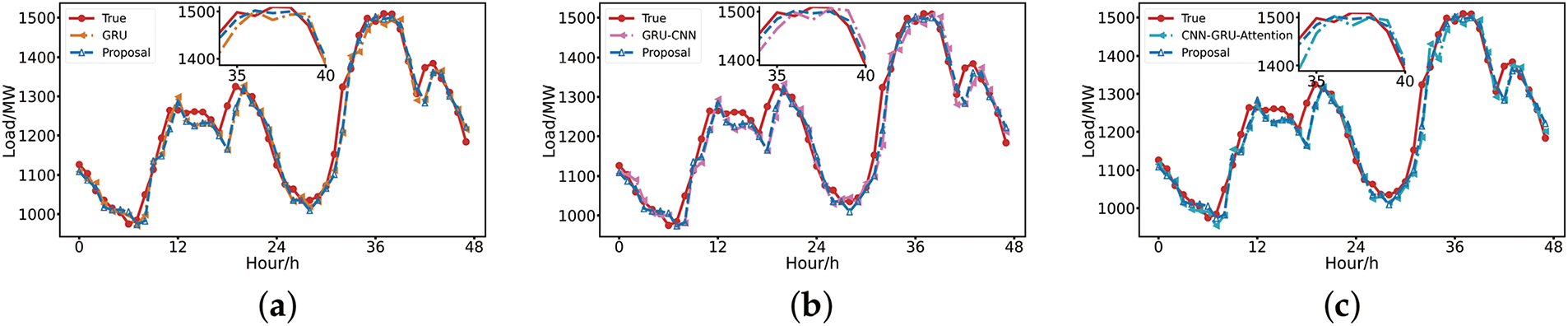
Figure 9: (a) Baseline model prediction curve comparison; (b) Combined models predict curve contrast; (c) Comparison of prediction curves of the influence of Attention mechanism on model effect

5  Conclusion

Short-term load forecasting is crucial for grid operation. This paper presents a power load forecasting method using T-CFSFDP clustering and BiGRU-CBAM, where T-CFSFDP clusters historical data first to underpin subsequent forecasts, CBAM heightens BiGRU’s focus on important data, and model integration improves adaptability to different data categories. Analysis reveals that compared with most mainstream models, it performs outstandingly in all metrics, with MSE, MAPE, MAE, and RMSE averaging improvements of about 21.72%, 5.94%, 8.33%, and 11.53%, respectively, demonstrating better accuracy. However, the current study has limitations such as the need to optimize model efficiency for real-time forecasting and the lack of consideration for short-term factors like weather and electricity prices that can cause short-term load fluctuations and affect prediction accuracy. Thus, future research can optimize the algorithm structure and use parallel computing to enhance model efficiency, incorporate more short-term influencing factors and multi-source heterogeneous data along with in-depth data fusion study, and integrate other advanced machine or deep learning methods to better handle complex load forecasting scenarios.

Acknowledgement: The editors and anonymous referees whose comments and recommendations have helped to improve this work are greatly appreciated by the authors. The authors would like to express their gratitude for the guidance and support provided by the research group.

Funding Statement: This work was supported in part by the Fundamental Research Funds for the Liaoning Universities (LJ212410146025), and the Graduate Science and Technology Innovation Project of University of Science and Technology Liaoning (LKDYC202310).

Author Contributions: Mingliang Deng: Writing—original draft, Methodology, Formal analysis, Data curation. Zhao Zhang: Review and editing, Conceptualization, Supervision. Hongyan Zhou: Investigation, Writing—editing. Xuebo Chen: Project administration, Reviewing. All authors reviewed the results and approved the final version of the manuscript.

Availability of Data and Materials: Data and materials are available upon request.

Ethics Approval: Not applicable.

Conflicts of Interest: The authors declare no conflicts of interest to report regarding the present study.

References

1. Panda SK, Jagadev AK, Mohanty SN, Vasant P. Forecasting methods in electric power sector. Int J Energy Optimizat Eng. 2018;7(1):1–21. doi:10.4018/IJEOE. [Google Scholar] [CrossRef]

2. Sanstad AH, McMenamin S, Sukenik A, Barbose GL, Goldman CA. Modeling an aggressive energy-efficiency scenario in long-range load forecasting for electric power transmission planning. Appl Energy. 2014;128:265–76. doi:10.1016/j.apenergy.2014.04.096. [Google Scholar] [CrossRef]

3. Chen Y, Xu P, Chu Y, Li W, Wu Y, Ni L, et al. Short-term electrical load forecasting using the Support Vector Regression (SVR) model to calculate the demand response baseline for office buildings. Appl Energy. 2017;195:659–70. doi:10.1016/j.apenergy.2017.03.034. [Google Scholar] [CrossRef]

4. Shang C, Gao J, Liu H, Liu F. Short-term load forecasting based on PSO-KFCM daily load curve clustering and CNN-LSTM model. IEEE Access. 2021;9:50344–57. doi:10.1109/ACCESS.2021.3067043. [Google Scholar] [CrossRef]

5. Hartless G, Booth JG, Littell RC. Local influence of predictors in multiple linear regression. Technometrics. 2003;45(4):326–32. doi:10.1198/004017003000000140. [Google Scholar] [CrossRef]

6. Qiu X, Zhang L, Suganthan PN, Amaratunga GAJ. Oblique random forest ensemble via least square estimation for time series forecasting. Inf Sci. 2017;420(2):249–62. doi:10.1016/j.ins.2017.08.060. [Google Scholar] [CrossRef]

7. Graves A. Generating sequences with recurrent neural networks. arXiv:1308.0850. 2013. [Google Scholar]

8. Kang K, Sun H, Zhang C, Carl B. Short-term electrical load forecasting method based on stacked auto-encoding and GRU neural network. Evol Intel. 2019;12(3):385–94. doi:10.1007/s12065-018-00196-0. [Google Scholar] [CrossRef]

9. Tang X, Dai Y, Liu Q, Dang X, Xu J. Application of bidirectional recurrent neural network combined with deep belief network in short-term load forecasting. IEEE Access. 2019;7:160660–70. doi:10.1109/ACCESS.2019.2950957. [Google Scholar] [CrossRef]

10. Xu A, Chen J, Li J, Chen Z, Xu S, Nie Y. Multivariate rolling decomposition hybrid learning paradigm for power load forecasting. Renew Sustain Energ Rev. 2025;212:115375. doi:10.1016/j.rser.2025.115375. [Google Scholar] [CrossRef]

11. Qian Y, Zhu Z, Niu X, Zhang L, Wang K, Wang J. Environmental policy-driven electricity consumption prediction: a novel buffer-corrected Hausdorff fractional grey model informed by two-stage enhanced multi-objective optimization. J Environ Manag. 2025;377:124540. doi:10.1016/j.jenvman.2025.124540. [Google Scholar] [PubMed] [CrossRef]

12. Li J, Chen J, Chen Z, Nie Y, Xu A. Short-term wind power forecasting based on multi-scale receptive field-mixer and conditional mixture copula. Appl Soft Comput. 2024;164(13):112007. doi:10.1016/j.asoc.2024.112007. [Google Scholar] [CrossRef]

13. Cui X, Zhang X, Niu D. A new framework for ultra-short-term electricity load forecasting model using IVMD-SGMD two-layer decomposition and INGO-BiLSTM-TPA-TCN. Appl Soft Comput. 2024;167(7):112311. doi:10.1016/j.asoc.2024.112311. [Google Scholar] [CrossRef]

14. Wang C, Li X, Shi Y, Jiang W, Song Q, Li X. Load forecasting method based on CNN and extended LSTM. Energy Rep. 2024;12(11):2452–61. doi:10.1016/j.egyr.2024.07.030. [Google Scholar] [CrossRef]

15. Luo S, Wang B, Gao Q, Wang Y, Pang X. Stacking integration algorithm based on CNN-BiLSTM-Attention with XGBoost for short-term electricity load forecasting. Energy Rep. 2024;12:2676–89. doi:10.1016/j.egyr.2024.08.078. [Google Scholar] [CrossRef]

16. Zou J, Li P, Su S, Shen X. Time series weighted density peak clustering algorithm and electric power load characteristic classification model. J Yunnan Univ: Nat Sci Edit. 2024;46(2):237–45. [Google Scholar]

17. Woo S, Park J, Lee JY, Kweon IS. CBAM: convolutional block attention module. In: Ferrari V, Hebert M, Sminchisescu C, Weiss Y, editors. Computer vision-ECCV 2018. ECCV 2018. Lecture notes in computer science. Vol. 11211. Cham, Switzerland: Springer; 2018. p. 3–19. [Google Scholar]

18. Rodriguez A, Laio A. Clustering by fast search and find of density peaks. Science. 2014;344(6191):1492–6. doi:10.1126/science.1242072. [Google Scholar] [CrossRef]

19. Mehmood R, Zhang G, Bie R, Dawood H, Ahmad H. Clustering by fast search and find of density peaks via heat diffusion. Neurocomputing. 2016;208(22):210–7. doi:10.1016/j.neucom.2016.01.102. [Google Scholar] [CrossRef]

20. Li C, Tang G, Xue X, Saeed A, Hu X. Short-term wind speed interval prediction based on ensemble GRU model. IEEE Trans Sustain Energy. 2019;11(3):1370–80. doi:10.1109/TSTE.2019.2926147. [Google Scholar] [CrossRef]

21. Li L, Jing R, Zhang Y, Wang L, Zhu L. Short-term power load forecasting based on ICEEMDAN-GRA-SVDE-BiGRU and error correction model. IEEE Access. 2023;11:110060–74. doi:10.1109/ACCESS.2023.3322272. [Google Scholar] [CrossRef]

22. Aguilar Madrid E, Antonio N. Short-term electricity load forecasting with machine learning. Information. 2021;12(2):50. doi:10.3390/info12020050. [Google Scholar] [CrossRef]

23. Wu L, Kong C, Hao X, Chen W. A short-term load forecasting method based on GRU-CNN hybrid neural network model. Math Probl Eng. 2020;2020:1–10. [Google Scholar]

24. Zhao B, Wang Z, Ji W, Gao X, Li X. A short-term power load forecasting method based on attention mechanism of CNN-GRU. Power System Technol. 2019;43(12):4370–6. (In Chinese). [Google Scholar]