Fuzzy Logic Based Evaluation of Hybrid Termination Criteria in the Genetic Algorithms for the Wind Farm Layout Design Problem

1  Introduction

The deterioration of climatic conditions globally, coupled with the depletion of fossil fuel resources, has promoted the use of renewable energy sources in recent years [1]. Scientists and engineers are working relentlessly to develop methods and technologies that improve the efficiency of renewable energy sources. One domain of renewable energy that has received notable interest from researchers is wind energy. There are several reasons to consider wind energy compared to traditional fossil fuel sources. The greatest advantage of wind energy is the financial aspect; the cost of generation, operations, and maintenance is substantially low [1]. In addition, the time frame in which a wind farm is developed and commissioned is much less than that of an energy generation facility that operates on gas, oil, or coal. Another factor that advocates the use of wind energy is that the wind is least affected by geographical boundaries and geopolitical conflicts. This is in contrast to fossil fuels which are owned and controlled by certain countries, and their movement from one point to another is heavily dependent on the logistical resources and geopolitical situation in the regions of interest.

Among the various challenges in the domain of wind energy research, efficient energy generation from a wind farm is the most crucial and focal issue. A factor that plays an important role in efficient energy generation is the layout of a wind farm, which governs the placement and configuration of wind turbines within the farm. Studies have shown that each potential wind farm has its own optimal configuration and a one-size-fits-all strategy does not work due to different topographical and climatic conditions [1]. This observation instigates the need to have techniques that can generate optimal layouts while considering site-specific information.

The wind farm layout design (WFLD) problem is classified as an NP-hard optimization problem [2]. As with many engineering problems, the WFLD problem has two main dimensions: the problem model and the computational model. A significant amount of work has been done on both dimensions during the past three decades. In terms of the engineering model, studies have proposed different wake models, placement strategies of turbines while treating the problem as a continuous or discrete optimization problem, modeling the problem as single-objective or multi-objective optimization, using different turbine types, and other factors such as site topography and climatic conditions. In terms of computational aspects, studies have focused on the use of nature-inspired algorithms (NIAs), which mainly consist of evolutionary computation and swarm intelligence algorithms, to solve the WFLD problem. In contrast to linear search or greedy algorithms, which are simple and computationally efficient, NIAs are computationally expensive. However, a major drawback of simple algorithms is that they often fail to produce efficient or even feasible solutions. This compelled researchers to resort to NIAs which stem from the domain of artificial intelligence and are capable of finding optimal or near-optimal solutions, but at a higher computational cost than simple algorithms. Some well-known NIAs that have been effectively applied to the WFLD problem include the genetic algorithms (GA), differential evolution (DE), particle swarm optimization (PSO), cuckoo search (CS), and many others. Mosetti et al. [3] were the first study to employ GA for the WFLD problem to extract the maximum energy for the minimum installation costs. Grady et al. [4] also developed a GA for maximum production capacity while limiting the number of turbines installed and the physical area occupied by each wind farm. With regard to DE, Rašuo et al. [5] utilized the algorithm for optimal placement of turbines on arbitrary configured terrains to achieve their maximum production effectiveness. Rašuo et al. [6] also proposed DE, while considering two different optimization functions. Rezk et al. [7] presented a comparative study involving DE and many other NIAs. Concerning PSO, Asaah et al. [8] combined the algorithm with a three-step strategy to improve the quality of a wind farm layout. Wu et al. [9] used PSO to design the optimal layout for a wind farm considering its noise, without sacrificing power production. Shin et al. [10] utilized a hybrid PSO for offshore WFLD. Afanasyeva et al. [11] developed a CS algorithm with auxiliary infrastructure and showed that infrastructure cost has an impact on the overall performance of the wind farm. In addition, Rezk et al. [7] applied the water cycle optimization algorithm, Kiamehr et al. [12] employed the imperialist competitive algorithm, and Aggarwal et al. [13] utilized biogeography-based optimization algorithm, all for the WFLD problem.

Traditionally, the NIA-based studies on the WFLD problem have primarily focused on improving/modifying the algorithm design to obtain better (and even optimal) solutions, without giving due consideration to the computational costs involved in the optimization process. An argument that can be given here is that computational time may be a critical issue in optimization problems that involve real-time decisions (such as scheduling), but for problems that do not involve real-time decisions, such as WFLD where the layout optimization is of the utmost importance, execution time is not important. From the problem engineering viewpoint, this argument is valid. However, in the computational sense, the principles of good algorithm design state that an efficient algorithm should be both time efficient and space efficient [14]. As such, an algorithm that only focuses on solution optimization without considering time optimization is not treated as an effective algorithm, irrespective of whether the problem solicits a real-time solution or not. In the context of time efficiency, a good algorithm is one that is executed just for the right time. That is, the algorithm is neither under-executed nor over-executed.

In terms of application of NIAs to the WFLD problem, the improvements and modifications were made mainly in two fundamental elements which are exploration and exploitation, and the researchers have paid significant attention to these two elements in almost all studies on WFLD. However, another aspect that deserves researchers’ attention is the algorithmic parameters that need to be properly tuned so that the algorithm can reach an acceptable (or optimal) solution in as little time as possible. One such important parameter is the algorithm’s termination condition, also referred to as the stopping criterion/criteria in the literature.

The stopping condition contributes to the execution of an algorithm so that the desired performance is achieved, and several studies have highlighted the importance of this issue [15,16]. If the algorithm stops prematurely, then a near-optimal/optimal solution may not be obtained which is an undesired scenario. In contrast, if the algorithm runs for a longer duration than what is needed, then the additional execution will result in a waste of resources. This situation has negative implications such as wasted execution cost (in terms of execution time utilization), unwarranted electricity consumption, and hardware stress. However, an inherent limitation of NIAs is that they cannot decide when to terminate the optimization process, and the automatic termination ability is not designed in the original versions of NIAs [15]. The primary reason for the lack of an automated termination process is that the problem solver is not often aware of the behavior of the NIA. To obtain an in-depth understanding of the behavior of an NIA, fitness landscape analysis (FLA) [17] is essential. The study of FLA falls in a different domain of research, generally outside the interest of researchers involved in studies on the WFLD optimization problem.

As mentioned above, the over-execution of an NIA results in waste of resources. The first and foremost is the overhead execution time. Since NIAs are iterative and non-deterministic, no notable improvement (or no improvement at all) may be observed for certain iterations during the execution, particularly towards the end of execution. However, computational resources are engaged in computations during such periods. In a uni-processor environment, the processor cannot accept a new processing job if the current process is in progress, and therefore other processes are delayed. With modern computational trends in which cloud computing is used, the wastage of computational resources is a more serious issue since the user pays a monetary cost to utilize computational time. More computational time means more financial cost, which is undesired. Furthermore, additional memory is required to keep the data generated during the overhead execution time.

Another concern is the unwarranted electricity consumption by the computing platform that arises due to additional execution of the algorithm beyond what is needed. Not only this, the additional electricity consumption leads to additional heat dissipation, which requires cooling. Thus, more electricity is required to manage the cooling systems. Furthermore, prolonged usage of a central processing unit (CPU) results in hardware stress, thus reducing the CPU’s lifetime [18,19]. Therefore, contemporary trends in software design and hardware architectures focus on green computing, leading to energy-aware algorithm design and computational platforms where the objective is to conserve as much energy as possible. This is achieved through energy-aware computing [20], energy-aware simulations [21], energy-aware software development [22], and other relevant methodologies. Numerous contemporary studies have incorporated energy-aware algorithms in various domains, signifying the importance of the issue.

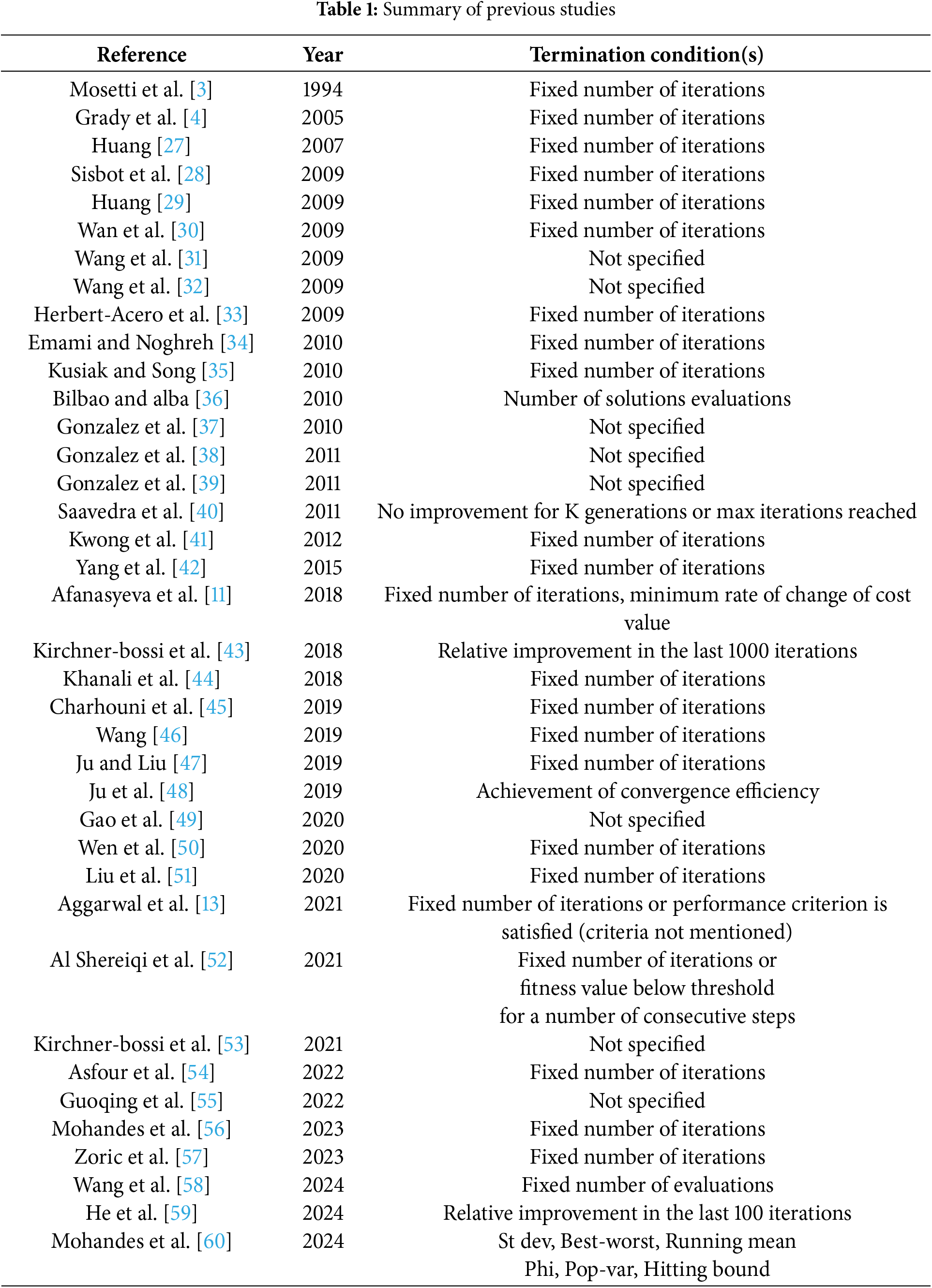
Ghoreishi et al. [15] reported that over 25 different stopping criteria have been used in studies involving NIAs in various domains. However, in the case of NIAs, as applied to the WFLD problem, only a few have been used. GA is particularly selected as an example since it has been the most utilized algorithm for the WFLD problem in the past [2] and is still actively used for the underlying problem. Furthermore, GA is a versatile algorithm and has been effectively used to solve a variety of optimization problems related to wind energy [23,24]. The table indicates that a huge majority of these studies have employed fixed number of iterations (FNI), without giving due consideration to the different wind scenarios encountered in the studies. As such, no justifications have been provided for the selection of the FNI termination criterion. In FNI, the user provides the number of iterations, and once the algorithm reaches the defined number of iterations, the execution is terminated. However, as pointed out by Ravber et al. [25], the FNI approach has several limitations and is therefore not a good approach for solving optimization problems with evolutionary algorithms, as well as GAs. A somewhat modified version of the FNI approach is the K-iterations (KIt) termination criterion. In KIt, the algorithm is terminated when no improvement is observed in the best fitness value through a K number of consecutive iterations. However, the user has to provide the value of K [26]. A review of studies on the use of GA for the WFLD problem between the period 1994 and 2024 is presented in Table 1.

In contrast to FNI and KIt, there are methods in which the termination is governed by the convergence of the search process. Some well-known examples are Standard Deviation [61], Best-Worst [61], Running Mean [61], Phi [61], Pop-Var [26], and Hitting bound [61]. However, these methods have their limitations; they also require certain threshold values to be defined by the user. These values are often not known a priori, thus making their use as termination criteria less appealing. To address this concern, Mohandes et al. [60] carried out a preliminary study to evaluate several termination criteria for the WFLD problem, but the results required further analysis for concrete outcomes and conclusions.

From the above observation and discussion, several research gaps can be identified. There is a need to assess the impact of termination criteria on the performance and convergence of an NIA. This assessment should not only focus on the quality of solutions generated by an NIA, but should also give due consideration to the computational aspects of a given algorithm. As such, this solicits a comprehensive comparison of several termination criteria while considering various wind scenarios. Furthermore, there exists a need to develop new termination criteria to increase the efficiency of the existing termination criteria. Motivated by the above observations and citing the limitations of the FNI termination criterion, this study strives to further analyze several termination criteria in the context of the WFLD problem. Accordingly, the novel aspects and key contributions of this study are enumerated as follows:

1.   Further insights are presented on the various hybrid termination criteria developed by Mohandes et al. [60] in the context of the genetic algorithm for the WFLD problem. The standard genetic algorithm is employed, as used in several past studies. It is worth mentioning that although the test bench is GA, the criteria are generic and can be used with any NIA in the domain of evolutionary computation or swarm intelligence and with any wake model with minor modifications in the algorithms employed.

2.   A fuzzy logic-based decision measure is proposed that combines the quality of the solution (i.e., Efficiency, as defined in Section 4) and the execution time consumed by the genetic algorithm. For this purpose, fuzzy membership functions for efficiency and execution time are developed and aggregated using the fuzzy arithmetic mean operator. Again, the approach can be used with any NIA without any difficulty.

3.   A comparative empirical study is carried out using various commonly employed wind scenarios while utilizing synthetic and real data. These wind scenarios primarily evaluate the impact of different wind speeds and wind directions on the algorithm’s performance. The possible correlation between a termination criterion and the given wind scenario is explored. It should be noted that any wind scenario with real or hypothetical data can be used without modification to the problem model or the algorithm design.

The rest of the paper is organized as follows. The problem background and model are presented in Section 2. This is followed by a discussion of genetic algorithms and termination criteria in Section 3. The proposed termination criteria are also discussed in Section 3. The fuzzy logic-based selection of termination criteria is presented in Section 4. In Section 5, empirical results are discussed. The paper ends with a conclusion and future research directions in Section 6.

2  Problem Background and Model

Since this study is oriented towards the algorithm design (in the context of the genetic algorithm), and not towards the problem model, the WFLD problem and related concepts are briefly described in this section for the sake of comprehensiveness. First, a primer on the WFLD problem is provided. This is followed by a short discussion on the wake model as well as the optimization function used in the study.

2.1 Wind Farm Layout Design Problem

The WFLD problem is concerned with placing the wind turbines in an optimal configuration within a wind farm. This optimal placement is vital for minimizing power loss due to different phenomena such as turbulence, wake decay, and transmission line loss. In addition, an optimal placement of wind turbines significantly affects the costs associated with the installation, operations, and maintenance of these turbines. In broader terms, the wind farm layout design problem can be defined as follows [2]:

“Given the location of a wind farm and the number of wind turbines, the aim is to place the turbines in the wind farm such that the design objective(s) are optimized while satisfying the design constraint(s).”

A wind farm is categorized as a geographical area that has a strong wind corridor and is therefore capable of producing wind energy through the use of wind turbines. Studies have proposed several wind farm layout structures based on the nature and topography of the terrain. The most prevailing model for a wind farm used in several studies assumes a discrete search space, where the farm is constituted of a planar area in a square form. This square is divided into 100 equally sized cells in a 10 × 10 grid configuration as shown in Fig. 1. These 100 cells lead to 2100 possible solutions [2], thus classifying the WFLD problem as an NP-hard problem. Turbines are placed in the middle of a cell while ensuring that a distance of 3D to 5D (where D is the turbine diameter) is maintained between turbines in all directions.

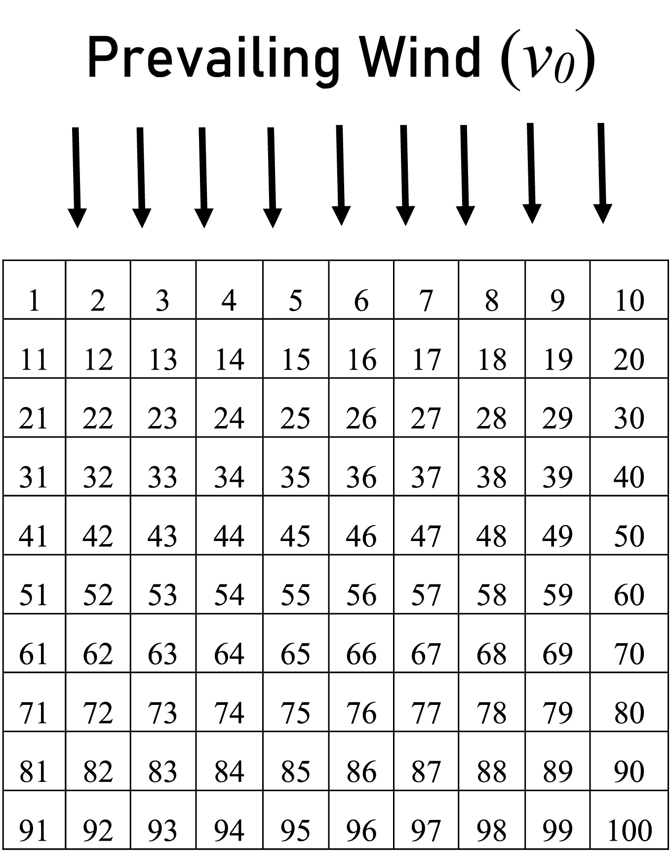
Figure 1: A 10 × 10 grid for placing turbines

2.2 Wake Modeling

Studies have proposed various wake-effect models, such as the Jensen model [62], the Katic model [63], the Frandsen model [64], two-dimensional wake model [65], three-dimensional wake model [66], Gaussian wake model [67], and PARK wake model [68]. In this study, we adopt the wake-effect model used in a recent study by Ju and Liu [47]. This wake effect model is derived from the two most established models which are the Jensen model [62] and the Katic model [63]. The study of Mosetti et al. [3] was the first to use the Jensen model and characterized the phenomenon of wake effect quantitatively. Furthermore, the model in Katic et al. [63] can strike a better balance between positive and negative errors and this wake model is widely used in literature [47].

Assume N turbines are to be placed in the wind farm. The prevailing wind has a speed of v0 as shown in Fig. 1. The turbines directly facing the wind are under no-wake effect. Therefore, wind speed remains unaffected at these turbines. Turbines that are affected by the wake encounter a wind speed of vi (i=1,2,…N) and vi < v0. The value of vi depends on whether a turbine is affected by a single wake or multiple wakes. If a turbine is affected by the wake of a single turbine, the mathematical representation to calculate this wake is given by the following equation [47]:

vi,j=v0[1−23(Rjrj)2](1)

where vi,j represents wind speed at turbine i under the wake effect of turbine j, and Rj is the rotor radius of the wind turbine j. Furthermore, rj is the wake radius and is represented as follows [47]:

rj=Rj+αdi,j(2)

In Eq. (2), α denotes the entrainment factor while di,j is the downward distance.

If a turbine i is affected by multiple wakes, the following equation is used to calculate this wake [47].

vi=v0[1−∑j∈Φj(1−vi,jv0)2](3)

where Φi is a set that includes all indices of turbines that are upwind of turbine i. A detailed discussion on the single and multiple wake models can be found in the study by Ju and Liu [47].

2.3 Optimization Model

As stated earlier, the purpose of the present study is not to evaluate the optimization model or its effectiveness. Therefore, only necessary details are provided herein. For details of the optimization model, the interested reader is referred to the study by Ju and Liu [47].

The number of wind turbines in the wind farm is assumed to be fixed and the direction of the wind is known. With these conditions, the aim is to harness wind energy with maximum efficiency. Therefore, the objective function is defined to maximize the conversion efficiency, represented as follows [47]:

maximize Efficiency=PcurrentPtotal(4)

where Pcurrent is the total power generated by turbines under the wake effect in the current layout and Ptotal is the ideal total power generated by all turbines without the impact of any wake.

3  Genetic Algorithm and Termination Criteria

This section focuses on the use of termination criteria for GAs. The section first describes GA and its structure. This is followed by a discussion on several termination criteria that have been employed in studies. The section then discusses the termination criteria adopted in the context of the WFLD problem.

3.1 Genetic Algorithms

The genetic algorithm is an iterative algorithm based on the theory of evolution. The algorithm was originally proposed by Fraser [69] in 1957 but received popularity through the work by Holland [70]. GAs operate on a set of solutions in parallel. The set of solutions is referred to as a population. Each solution, commonly referred to as a chromosome, is represented by a string of symbols. A chromosome consists of individual elements known as genes. During each iteration, a new set of chromosomes, called offspring, is generated.

The effectiveness of search in GA depends on two processes: exploration and exploitation [71]. Exploration is concerned with traversing the search space with the aim of discovering new regions therein. Exploitation is connected with fine-turning the search, focusing on a directed search in a smaller region of the search space. To make GA carry out the search efficiently, a balance between both processes is crucial during the search. A high level of exploration can lead to inefficient search since the algorithm is prone to missing good solutions, resulting in a higher execution time to reach convergence. In contrast, a high level of exploitation can cause a loss of population diversity and may lead to premature convergence, thus resulting in low-quality solutions [72,73].

The exploration and exploitation in GA are controlled by two distinct mechanisms known as crossover and mutation. Crossover is responsible for exploitation and is controlled by a parameter called the ‘crossover rate’. Similarly, exploration is controlled by another parameter known as the ‘mutation rate’. The values of these two parameters are user-defined. For GA to reach convergence to produce an optimal solution, an ample amount of time (and equivalently, the number of iterations) is required so that both exploration and exploitation are fully utilized. However, as stated in Section 1, both over-execution and under-execution of an NIA, vis-a`-vis a GA, are not desired. This leads to the incorporation of different termination criteria in GA as discussed below. The objective is to determine which termination criterion best achieves just the right number of iterations. Fig. 2 shows the flowchart of GA employed for the WFLD problem.

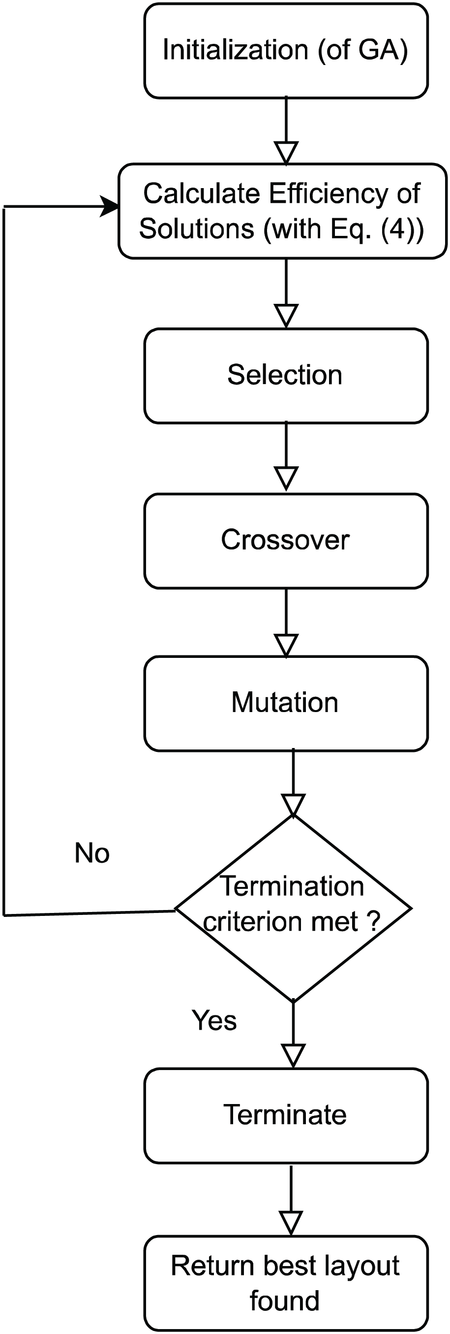
Figure 2: Flowchart of GA based approach for the WFLD problem

3.2 Termination Criteria in WFLD Problem

As mentioned in Section 1, several termination criteria have been proposed in the literature, but not utilized in the context of the WFLD problem. Some well-known examples are Standard Deviation, Best-Worst, Running Mean, Phi, Pop-Var, and Hitting bound criteria. These are explained below.

The Standard deviation (St dev) based termination criterion [61] measures the standard deviation of the fitness values of all solutions in the current iteration. The execution stops if this standard deviation is equal to or less than a predefined threshold value λ ≥ 0 set by the user.

The best-worst termination criterion [61] works on the difference between the best and the worst fitness values in the current iteration. Once this difference is equal to or less than a predefined threshold value λ≥ 0, the execution of GA stops. This threshold is predefined by the user.

The running mean termination criterion [61] is fulfilled if the difference between the best fitness value of the current iteration and the average of the best fitness values in the last tlast iterations is equal to or less than a given threshold λ ≥ 0.

The Phi termination criterion [61] is satisfied if the quotient of the best fitness value and the mean of all fitness values of the current iteration is equal to or greater than a given threshold 1 − λ, where 1 ≫ λ ≥ 0. Once this condition is satisfied, the algorithm stops.

The Pop-var termination criterion [26] deals with the variance in the current population. The algorithm terminates once the variance of fitness values of all individuals in the current population becomes equal to or less than a given threshold 1 ≫ λ ≥ 0.

In the hitting bound termination criterion [61], the best value of the fitness function is defined by the user. Once this best fitness value by any solution is obtained, the algorithm terminates. In this case, it is expected that the found solution is close enough or equal to the known global optimum.

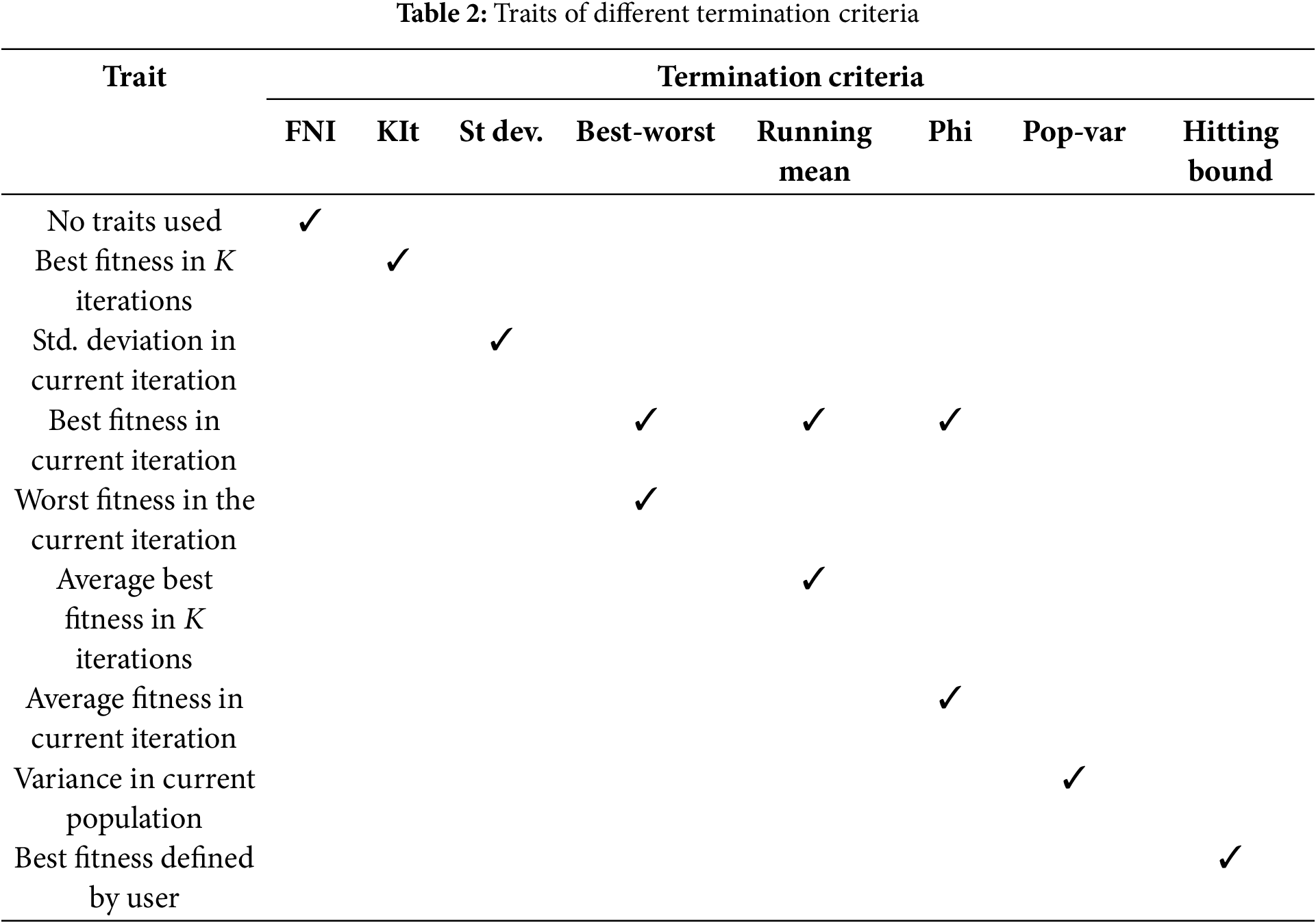
Table 2 summarizes the traits used in different termination criteria. Based on the information in the table, the termination criteria can be divided into two groups. The first group consists of criteria that have a single trait. Examples of these criteria are St dev, Pop-var, and Hitting bound. The second group consists of the criteria having two traits. Best-worst, Running mean, and Phi are examples of these termination criteria.

3.3 Modified Hybrid Termination Criteria

One obvious and common limitation of most of the aforementioned termination criteria is that the threshold value of λ that triggers the termination of GA has to be defined by the user. In most cases, determination of the best threshold value of λ is cumbersome. In addition, certain other factors, such as the standard deviation of the population, the difference between the best and worst fitness values, the mean fitness of the solutions in the current iteration, and other simulation-dependent parameters, are not known to the user a priori. In the context of the WFLD problem, getting specific information such as the optimal fitness value, the iteration best/worst values, defining the bound, identifying a certain standard deviation or population variance, and other such variables are not possible until the simulation is carried out. This again raises the question of how to terminate the algorithm if problem-specific information is not available or not known. This issue was somewhat addressed by Mohandes et el. [60] by adopting an approach in which the uncertainties about the termination process are at least minimized, if not completely alleviated. They achieved this by utilizing the K-iterations (KIt) termination as identified in Section 1. The KIt criterion ensures termination at a definite instance, provided that the algorithm reaches a stable state where no further improvements are observed in the solution. However, KIt itself cannot be used alone since it is not known in advance as to when the algorithm would achieve convergence. This led to the development of hybrid termination criteria. A brief discussion of these hybrid termination criteria is provided below for the sake of completeness. Further details can be found in Mohandes et al. [60].

The modified criteria evolve from the hybridization between the basic criterion and KIt. With regard to the hybrid standard deviation criterion, the standard deviation of the fitness values of all solutions in the current iteration is calculated. These fitness values are recorded for each iteration. If the standard deviation does not change (remains constant) for K consecutive iterations, then it signifies that the algorithm has reached convergence and no further diversity is possible in the population. Eventually, the execution of the algorithm stops. In the same sense, the hybrid best-worst approach monitors the difference between the best and worst fitness values in the current iteration. The algorithm terminates if the difference between these two extremes does not change for K consecutive iterations. The hybrid running-mean criterion is satisfied if the difference between the best fitness value of the current iteration and the average of the best fitness values in the last tlast iterations does not change for k consecutive iterations. In the hybrid Phi criterion, termination is reached if the quotient of the best fitness value and the mean of all fitness values of the current iteration remains the same for K consecutive iterations. Likewise, in the hybrid Pop-var approach, the algorithm terminates when the variance of the fitness of solutions in the current population does not change for K consecutive iterations. Finally, in the hybrid hitting bound criterion, the user defines the threshold of the best fitness value. Once this threshold is achieved by any solution and remains constant for K consecutive iterations, the algorithm terminates.

4  Fuzzy Logic Based Selection of Best Termination Criterion

Eq. (4) represents the efficiency of the wind farm. This efficiency denotes the fitness function in GA. If only efficiency is used as the measure for deciding the best termination criterion, there are no confusion or uncertainties. The decision could simply be taken by selecting the termination approach that leads to the best (maximum) efficiency. The problem arises when the execution time is also taken into account. Consider, for example, the following scenario in which the efficiency and execution time of two hypothetical termination criteria are given. From the data in Table 3, we see that termination criterion A has a higher efficiency (as desired) than criterion B, but also has inferior performance in terms of execution time, showing 150 s (which is 20 s more than that of criterion B), indicating an undesirable situation. So, criterion A is better in terms of efficiency, and criterion B is better in execution time. The question is, which one of these criteria is overall better than the other while considering both efficiency and execution time equally important? With the human-based approach, such a decision would be difficult as the approach creates uncertainties in the decision. This motivates us to utilize multi-attribute decision-making (MADM) methods (also referred to as multi-criteria decision-making or MCDM) which stem from the domain of artificial intelligence.

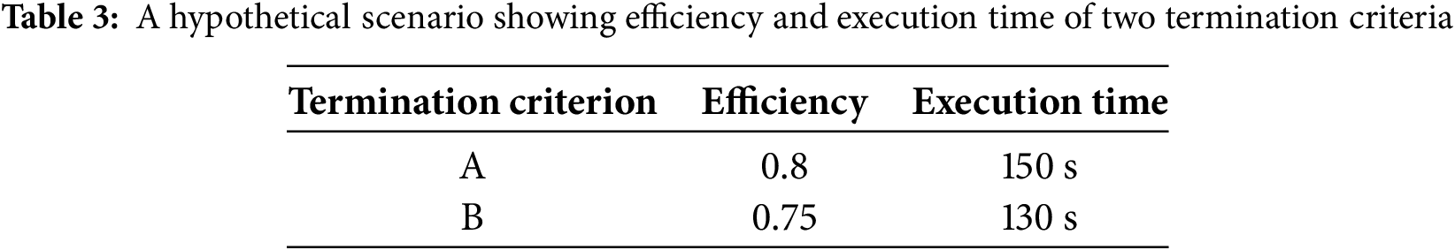
The MADM methods are employed in decision problems involving multiple attributes in the decision-making process. These attributes are both mutually conflicting and incommensurable [1]. Conflict represents a scenario in which improvement in the quality of a decision in one criterion negatively affects the decision on at least one other decision criterion. Incommensurability refers to attributes having different units and magnitudes. In the example in Table 3, criterion A achieved better efficiency, but at the cost of more execution time which shows a conflicting situation. Furthermore, efficiency has no units and is scaled between 0 and 1, whereas execution time is measured in seconds and could have magnitudes in multiple digits.

In the literature, several MADM methods have been proposed. Some well-known methods include weighted sum, lexicographic ordering, ϵ-constraint method, goal programming, goal attainment, and fuzzy logic. In comparison with fuzzy logic, other methods have several limitations. For example, in the weighted sum method, a small change in weights may result in big changes in the objective vectors. In lexicographic ordering, the main disadvantage is that the method tends to favor certain objectives when many are present, as the decision-maker may have difficulty in defining the order of importance of objectives. The most prominent disadvantage of ϵ-constraint method is that the method is time-consuming. As for goal programming, the main disadvantage is that if the targets are not defined properly, the decision may be misleading. A similar concern goes with the goal attainment method. A detailed discussion on the limitations of the above methods can be found in Miettinen [74].

In contrast to the above methods, the MADM aspect associated with the underlying WFLD problem can be effectively addressed by utilizing the fuzzy logic-based approach. A strong reason to consider the fuzzy logic approach for the WFLD problem is that fuzzy logic conveniently deals with uncertainties in data associated with the underlying problem [1]. Furthermore, the problem-based domain information is easily represented through the concepts of natural language processing (NLP), since NLP can effectively handle human knowledge acquired through experience and understanding of problems [1].

The fuzzy logic-based MADM approach requires both attributes to be aggregated to form a decision function. This decision function, which is in the form of a mathematical equation, represents a decision rule. For the WFLD problem, an appropriate decision rule could be as follows:

Rule 1: IF Efficiency is increased AND Execution time is decreased THEN the Termination Criterion is effective.

In the above rule, Efficiency, Execution time, and Termination Criterion are the linguistic variables, each of which defines a fuzzy subset of solutions. To implement the above rule using fuzzy logic, membership functions for the linguistic variables have to be defined. A membership function returns a value in the interval [0, 1] which describes the degree of satisfaction with the decision criterion under consideration [1]. Using the arithmetic mean operator [75], Rule 1 translates to the following equation:

μC(x)=μE(x)+μT(x)2(5)

In Eq. (5), μC(x) defines the membership function for the Termination Criterion. Similarly, μE(x) and μT(x) represent the membership functions for Efficiency and Execution time, respectively. In order to calculate μC(x), both μE(x) and μT(x) need to be determined first, as explained below.

4.1 Membership Function for Efficiency

The membership function for Efficiency, μE(x), can be defined as follows. The two extreme values of Efficiency ‘Emax’ and ‘Emin’ define the maximum (ideal) and minimum values, respectively. Emax is taken as 1 while Emin is set at 0. The membership function for Efficiency is mathematically represented as follows.

μE(x)={1if E(x)≥EmaxE(x)−EminEmax−Eminif Emin≤E(x)<Emax0if E(x)<Emin(6)

where the term E(x) represents the Efficiency of the current solution.

4.2 Membership Function for Execution Time

The membership function for Execution time, μT(x), can be defined as follows. The values ‘Tmax’ and ‘Tmin’ define the maximum and minimum (ideal) execution time, respectively. The minimum value, Tmin is set at 0, indicating that the execution takes no time at all, which is an ideal (but hypothetical) scenario. The maximum time, Tmax is taken to be the highest execution time taken by any of the termination criteria. Then, the membership value for Execution time is determined as follows.

μT(x)={1if T(x)≤TminTmax−T(x)Tmax−Tminif Tmin<T(x)≤Tmax0if T(x)>Tmax(7)

where the term T(x) represents the execution time of the current solution.

5  Results and Discussion

In this section, the empirical results are presented and discussed to evaluate the performance of the various termination criteria proposed herein. In the majority of past studies on the WFLD problem, three standard scenarios were assumed. These included (a) wind with a single speed coming from a single direction, (b) wind with multiple speeds coming from a single direction, and (c) wind with multiple speeds coming from multiple directions. As such, simulations were carried out considering the above three scenarios, using real and hypothetical data. The real data was collected from a potential site of Turaif (located at a height of 827 meters above sea level) in Northern Saudi Arabia. A wind speed of 6.94 m/s at a height of 130 meters was used in the experimentation for Turaif [60]. The following wind scenarios were assumed:

•   Case 1: Wind speed of 6.94 m/s coming from a single direction.

•   Case 2: Wind speed of 6.94 m/s coming from four different directions.

•   Case 3: Wind speeds of 6.94, 10, and 12 m/s coming from 12 different directions.

Furthermore, after carrying out parameter sensitivity analysis, the parameters of the genetic algorithm were set as follows: population size = 30, crossover rate = 0.6, and mutation rate = 0.1. Other parameters used in the simulations included grid size = 10 × 10, number of turbines = 20, and K = 10.

As per the established approach suggested in the literature [2,76], all experiments were carried out with 30 independent runs, and results were reported as the average of best efficiency in 30 runs as well as standard deviations of these 30 runs, with the corresponding executions times. Furthermore, statistical validation was done using the Wilcoxon ranked-sum test at a 95% level of confidence. Note that GA (and likewise, any other algorithm from the domain of evolutionary algorithm and swarm intelligence) is a non-deterministic algorithm, and the result of a single run cannot lead to the best efficiency. As such, the layout generated by a single run cannot be used to reach a conclusion.

All experiments were done using the same initial solution (seed population) for GA. Furthermore, uniform simulation conditions (with regard to background processes and software platform) and hardware setup were used. Simulations were carried out using the Python programming language, where the open-source Python package developed by Ju and Liu [47] was used as the base code.

5.1 Effect of Termination Criteria on Efficiency

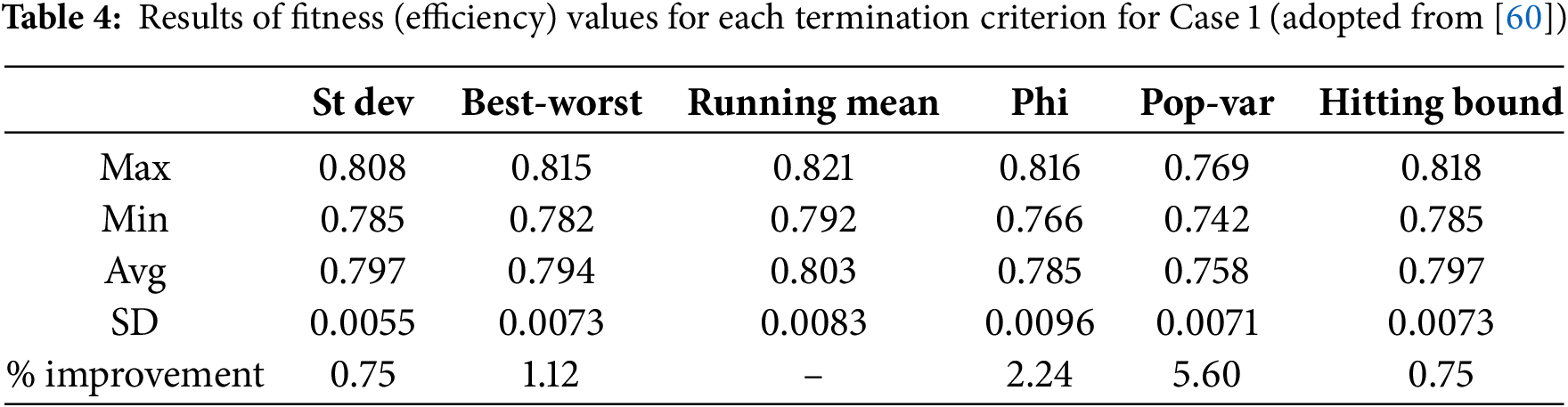
Tables 4–6 show the results obtained for Efficiency for the six termination criteria for Case 1, Case 2, and Case 3, respectively. With regard to Case 1, the results presented in Table 4 are adopted from Mohandes et al. [60] and are presented here for a comprehensive analysis. It is observed from Table 4 that the running mean termination criterion produced the best results. More specifically, the maximum values (0.821), minimum values (0.792) and average values (0.803) are all on the high sides compared to the results of the other termination criteria. However, the standard deviation (with a value of 0.0083) is relatively higher than many other termination criteria. On the other hand, if we look at the results produced by the St dev criterion, the results indicate a stable behavior since the standard deviation of the 30 runs is the lowest among all criteria, with a value of 0.0055. However, the maximum, minimum, and average values obtained by the St dev criterion are not impressive, as they fall on the lower side compared to the results for several other termination criteria. In short, the St dev criterion achieved improvements in the range of 0.75% to 5.60%.

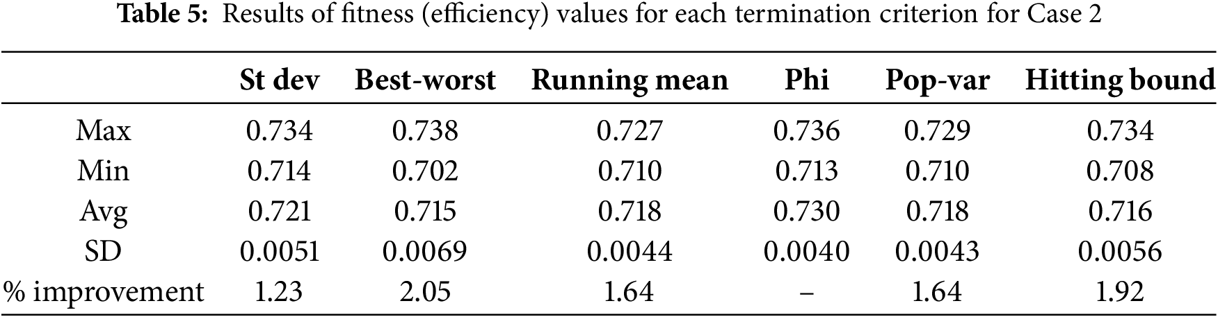
For Case 2, the results in Table 5 indicate that the Phi termination criterion was the best, with the highest average efficiency of 0.730. Furthermore, the standard deviation associated with the results of the criterion Phi is also the lowest among all other criteria, with a value of 0.0040. This performance translates to improvements in the range of 1.23% to 2.05% achieved by Phi.

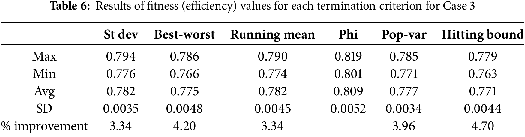
Finally, the termination criterion Phi is also the best for Case 3, as revealed by the results in Table 6. The average conversion efficiency for Phi is 0.809, with a standard deviation of 0.0052. Although this standard deviation is the highest among all criteria, it should be noted that even the minimum of Phi is greater than the maximum values obtained by all other criteria. Therefore, Phi is undoubtedly the best for Case 3, showing an improvement in the range of 3.34% to 4.70%.

Fig. 3 provides more details about the different termination criteria. The figure illustrates the distribution of the best solution for 30 runs with regard to each criterion for the three test cases. These solutions are distributed in five ranges of efficiency, which are 0.7 to 0.729, 0.73 to 0.759, 0.76 to 0.789, 0.79 to 0.819, and 0.82 to 0.849. These five efficiency ranges were carefully chosen to represent the sensitivity of the efficiency change for each termination criterion. As observed in Fig. 3a, Running mean has solutions in the topmost efficiency range (i.e., 0.82 to 0.849). That is, out of the 30 solutions generated during the 30 runs, Running mean had 2 solutions in the top efficiency range, while 28 solutions were in the second topmost range (0.79 to 0.819). Furthermore, the closest contenders to Running mean are the St dev and Hitting bound criteria which produced 29 solutions each in the second topmost range, with one solution each in the middle-efficiency range (0.76 to 0.789). In contrast, Pop-var showed the worst performance since the criterion resulted in no solution in the topmost efficiency range, with solutions distributed in the second topmost and the middle-efficiency range. However, in Case 2, all criteria (with the exception of Phi) produced huge number of solutions in the lowest range of 0.7 to 0.729, as can be seen in Fig. 3b. In contrast, Phi is the only criterion that had the majority of results in a higher efficiency range of 0.73 to 0.759. Finally, for Case 3, Fig. 3c clearly illustrates that only the Phi was able to generate all results in the second topmost efficiency range (0.79 to 0.819), while all other criteria produced results in the lower range of 0.76 to 0.789.

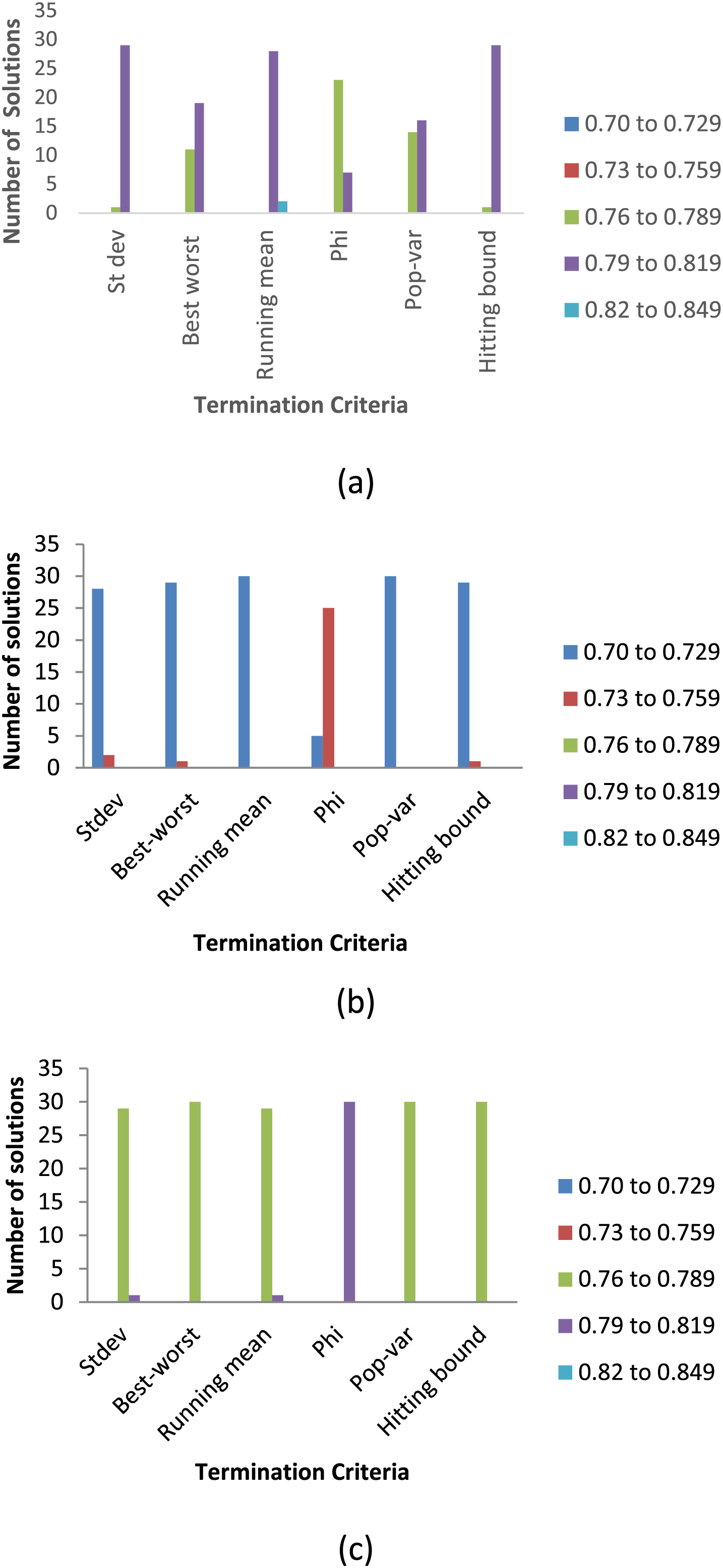
Figure 3: Distribution of efficiency in different ranges vs. termination criteria for (a) Case 1 (b) Case 2 and (c) Case 3

Fig. 4 shows the progression of efficiency vs. iteration for the three cases. The plots show the progression of the best run (out of the 30 runs) for each termination criterion. For Case 1 (Fig. 4a), it is observed that Running mean was able to achieve the best efficiency as the criterion allowed the algorithm to execute for a sufficient amount of time. In contrast, Pop-var caused GA to terminate in the very early stage of execution which did not allow the algorithm to properly search the solution space. With regard to Case 2, Best-worst achieved convergence in the very early stage, whereas Phi was also able to reach almost the same efficiency level, but at a later stage, as shown in Fig. 4b. In contrast, Pop-var made the algorithm execute for a very long duration, yet did not achieve the high efficiency level as that of other termination criteria. For Case 3, the best performance of Phi is visible in Fig. 4c where the criterion achieved the highest efficiency. This high level of efficiency was achievable since GA had ample time to converge.

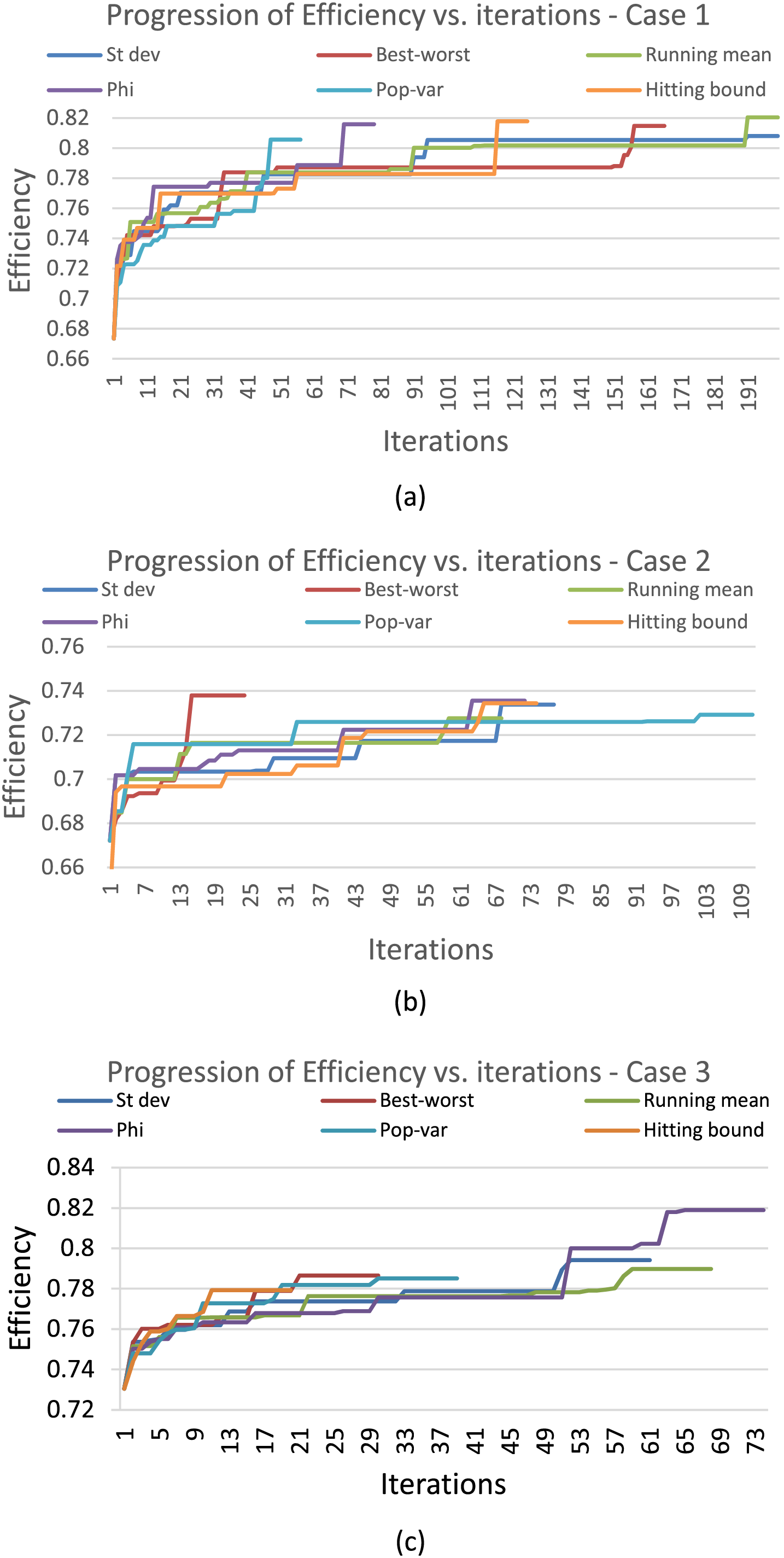
Figure 4: Progression of efficiency vs. iterations for (a) Case 1 (b) Case 2 and (c) Case 3

Based on the above observations, it can be fairly claimed that for Case 1, the Running mean termination criterion was the best among all since it has generated most of the results with the highest efficiency while maintaining a stable behavior as suggested by its small standard deviation associated with the results. Although St dev criterion had the lowest standard deviation, it was not able to produce enough results in the high-efficiency ranges. In contrast, the worst performer was Pop-var; despite a relatively low standard deviation, the solutions produced by the criterion in terms of efficiency were of the worst quality. For Cases 2 and 3, the Phi criterion was the best. For Case 2, the Best-worst approach was the worst, although comparable to Hitting bound, and for Case 3, Hitting bound was the worst.

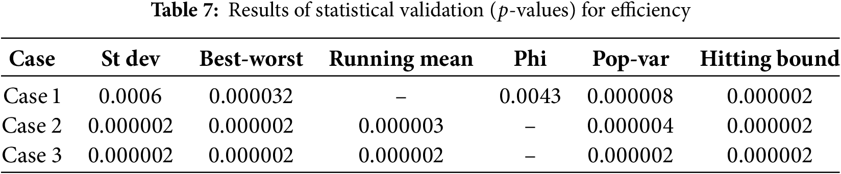
In order to further strengthen the claims about the best performers, statistical validation was also carried out. The p-values are shown for all three cases in Table 7. For Case 1, Running mean reflected the best output as reported in Table 4, and therefore this termination criterion was used as the benchmark. The p-values in Table 7 indicate that the fitness values (i.e., efficiency) of Running mean were statistically significant as compared to the other termination criteria since all p-values were less than 0.05. Similarly, for Cases 2 and 3, the Phi termination criterion was the best (statistically significant) among all other termination criteria. These outcomes prove the hypothesis that the termination condition has an impact on the quality of solutions produced in terms of efficiency.

5.2 Effect of Termination Criteria on Execution Time

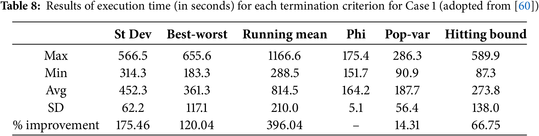
With regard to the impact of the termination criteria on the execution time, results of the 30 runs are summarized in Tables 8–10 for Case 1, Case 2, and Case 3, respectively. For Case 1 (adopted from Mohandes et al. [60]), it is visible from Table 8 that termination criterion Phi resulted in the lowest execution time with an average of 164.2 s with a standard deviation of just 5.1, which is also the lowest among all criteria. Although Pop-var had a minimum execution time of 90.9 s, the criterion cannot be declared as the best since the average execution time (187.7 s) and standard deviation of 56.4 s are much higher than that of Phi. Furthermore, the worst performer was the Running mean as the average execution time was the highest (814.5 s) with the highest standard deviation of 210 s. In terms of percentage improvements, Phi achieved values in the range of 14.31% to 396.04%.

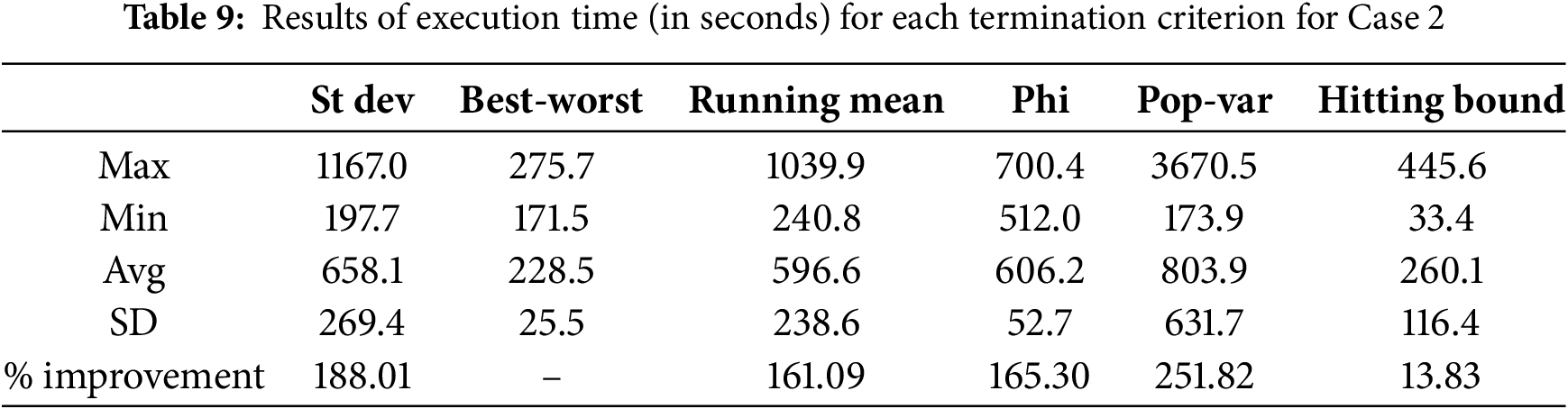
For Case 2, the Best-worst criterion resulted in the minimum execution time with an average of 228.5 s. The criterion also showed a standard deviation of 25.5 s, which was the lowest. The worst performer for Case 2 was Pop-var with an average execution time of 803.9 s and a standard deviation of 631.7 s. The percentage improvement achieved by Best-worst falls in the range of 13.83% to 251.82%.

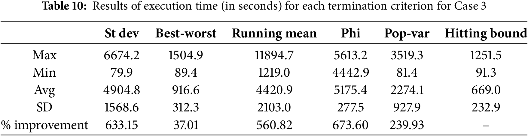
Finally, for Case 3, the criterion Hitting bound displayed the lowest average execution time of 669.0 s, while Phi was the worst with the highest average execution time of 5175.4 s. The standard deviation of Hitting bound was the lowest with 232.9 s, while that of Phi was 277.5 s. One interesting observation is for the Running mean criterion which has the highest run time of 11894.7 s, which is the highest among all criteria, as well as the highest standard deviation of 2103 s, indicating an unstable behavior of the criterion. This translates into improvements between 37. 01% and 673. 60% achieved by Hitting bound in comparison with other criteria.

A further analysis of the results in Fig. 5 gives more insight into the behavior of the criteria. For Case 1, Fig. 5a indicates that all solutions for Phi were spread in the low execution time spectrum (0 to 249 s), while the worst performer was Running mean with most of the solutions in the high execution time range (with 6 solutions in the range of 1000 to 1249 s and 13 solutions in the range of 750 to 999 s). For Case 2, as shown in Fig. 5b, only Best-worst had all its solutions in the range of 0–299 s, while Pop-var had some solutions above 1200 s. However, most of the solutions of Pop-var were spread among different ranges. For Case 3, Hitting-bound was the best since it had almost all its solutions in the range of 0 to 999 s, while all other criteria had solutions in higher ranges, particularly in the “Above 4000” s, as shown in Fig. 5c.

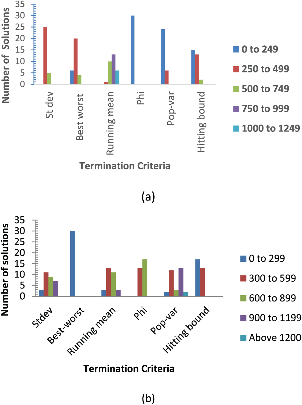
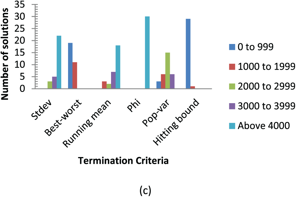
Figure 5: Execution time (in seconds) vs. termination criteria for (a) Case 1 (b) Case 2 and (c) Case 3

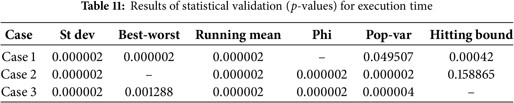
To obtain a more accurate picture, the statistical analysis in Table 11 reveals that for Case 1, the Phi criterion was the best among other criteria since the p-values of the criterion were always less than 0.05. This indicated that the difference in the runtime by Phi and other criteria was statistically significant. In Case 2, the difference in execution time between the Best-worst criterion and other criteria was statistically significant, indicating that the criterion was the best. An exception here was the Hitting-bound criterion where the p-value was 0.158865, indicating that both Best-worst and Hitting-bound were equally good, in statistical terms. Finally, for Case 3, the Hitting-bound criterion performed the best in terms of statistical significance, since all p-values were less than 0.05. Statistical testing indicates that termination criteria have an impact on the execution time of the algorithm.

5.3 Fuzzy Logic Based Decision for the Best Criterion

The results presented in Sections 5.1 and 5.2 suggest that in terms of conversion efficiency, Running mean was the best in Case 1, while Phi was the best in Cases 2 and 3. On the other hand, in terms of execution time, Phi was the best for Case 1, Best-worst for Case 2, and Hitting-bound for Case 3. This points towards a conflicting situation, whereby the decision about the best termination criterion with regard to both conversion efficiency and execution time couldn’t be clearly identified. As such, fuzzy logic-based approach proposed in Section 4 was employed to reach a concrete decision.

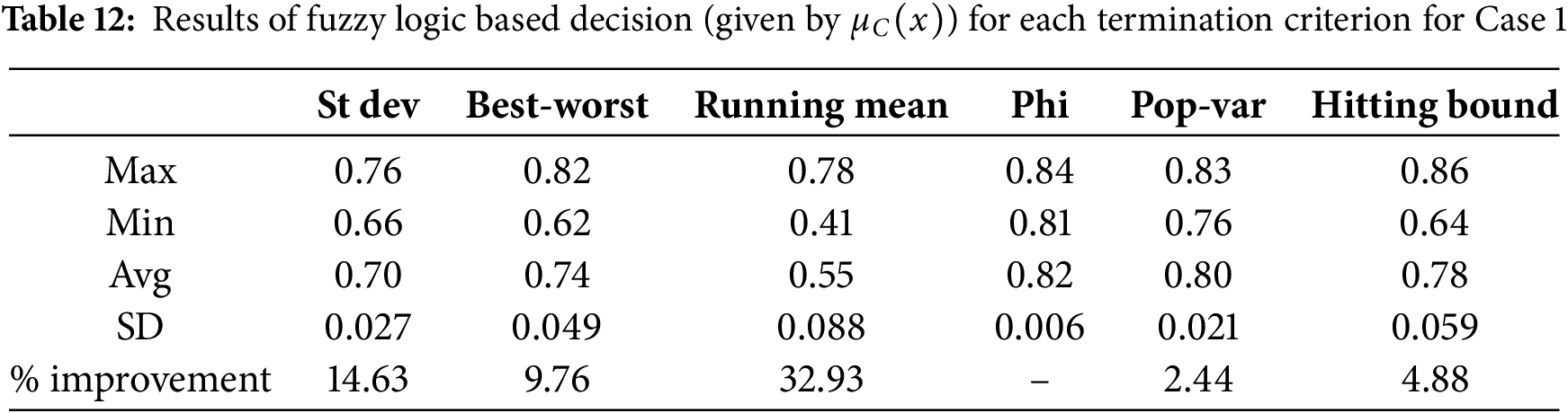
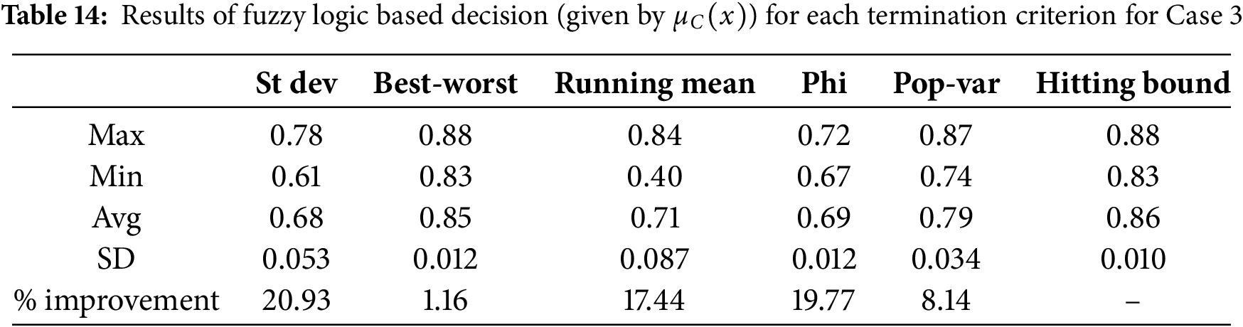
Tables 12–14 present the results of aggregation of Efficiency and Execution time using the fuzzy arithmetic mean operator, represented by μC(x) in Eq. (5), for Cases 1, 2, and 3, respectively. The results in Table 12 indicate that for Case 1, Phi turned out to be the overall best termination criterion since it had the fuzzy value (average) of 0.82 which was the highest among the fuzzy values of other criteria. This translates to an improvement in the range of 2.44% to 32.93% by Phi compared to other termination criteria. For Case 2, Table 13 signifies that Best-worst was the best option with a fuzzy value of 0.83. Although Hitting-bound is also comparable with a fuzzy value of 0.82, the criterion had a high standard deviation of 0.015 compared to 0.005 of Best-worst. The improvement achieved by Best-worst was in the range of 1.2% to 9.64%. As for Case 3, the best performer was Hitting-bound with a fuzzy value of 0.86 and a standard deviation of 0.010 as shown in Table 14. For Case 3, Best-worst was also the closest contender with a fuzzy value of 0.85 and a standard deviation of 0.012. Overall, Hitting-bound was the best performer for Case 3, reflecting an improvement between 1.16% to 20.93% compared to the other termination criteria.

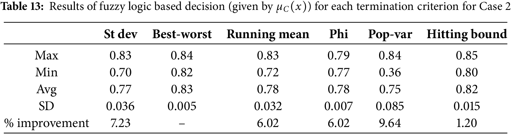
In terms of statistical validation, Table 15 indicates that Phi produced statistically significant results for Case 1 compared to all other criteria. For Case 2, Best-worst was the best, with the exception of Hitting-bound since the p-value was 0.298952, indicating that both Best-worst and Hitting-bound were equally good in terms of statistical significance. For Case 3, Hitting-bound was the best among all options.

5.4 Discussion

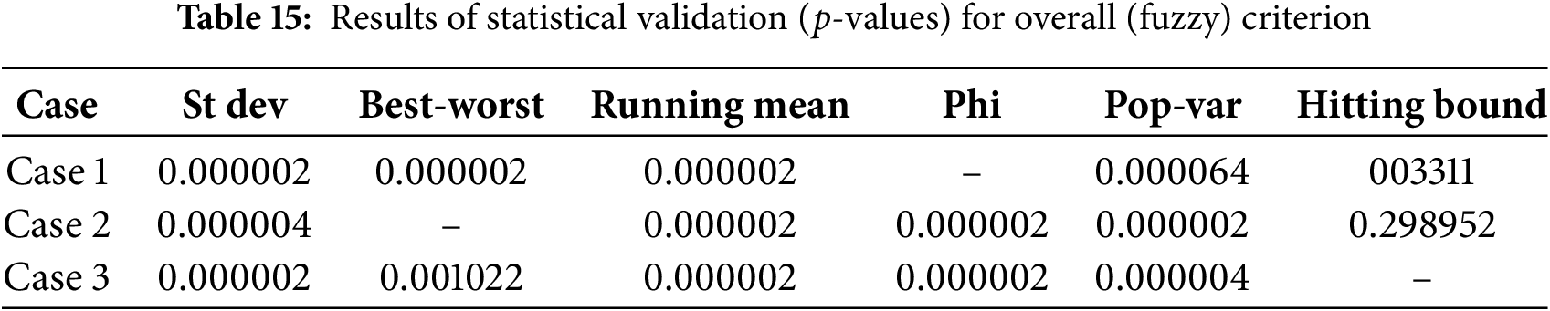
Based on the statistical analysis presented in Tables 7, 11, and 15, a summary of the best termination criteria is presented in Table 16. It is observed from Table 16 that for the given test scenarios, Running mean, Phi, Best-worst, and Hitting-bound produced the best results. One possible explanation for the superior performance of Phi, Best-worst, and Running mean can be attributed to the very structure of the said termination criteria. Note that the three termination criteria are governed by two traits as highlighted in Table 2. Furthermore, the common trait among the three criteria is the best fitness value. An exception was the Hitting-bound criterion, which is based on a single attribute. However, in general, termination criteria with a single trait showed poorer performance compared to termination criteria with multiple traits.

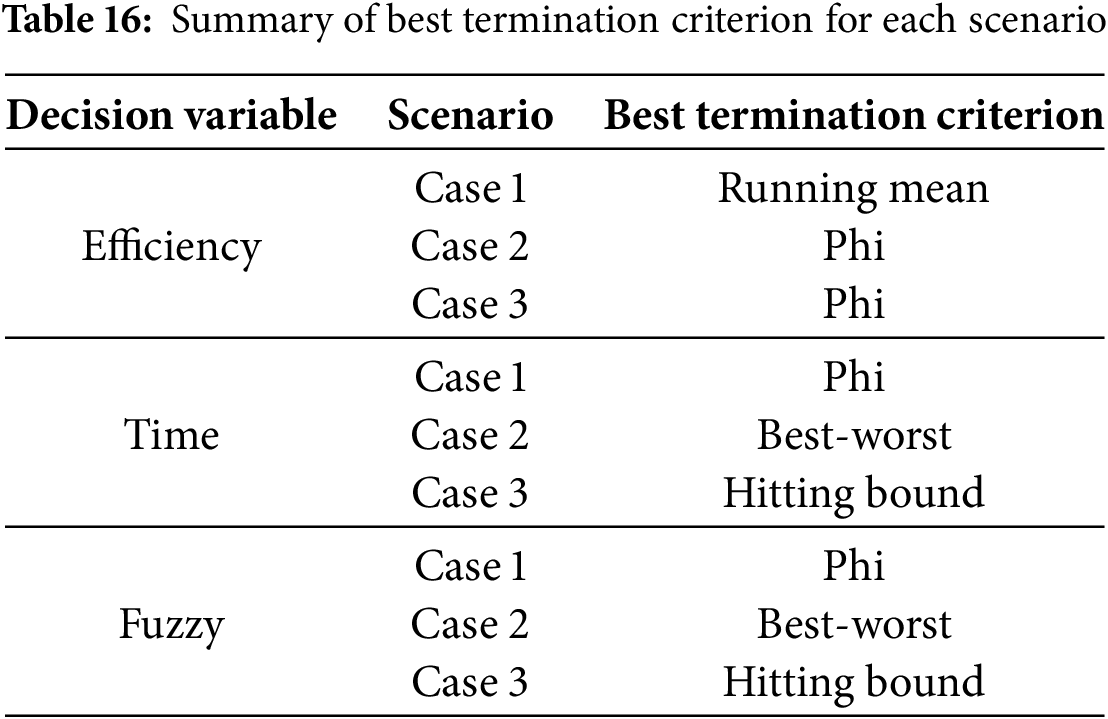
Another observation in Table 16 is that the overall decision (i.e., fuzzy decision criterion) is more influenced by the objective time objective rather than the fitness objective. That is, the best termination criterion for each case is the same for the time objective, as well as the fuzzy decision. This is interesting since both efficiency and time criteria were given equal preference in the decision-making using the arithmetic mean operator (Eq. (5)). To an extent, this also highlights the importance of the execution time in the optimization process for the underlying problem.

6  Conclusions and Future Directions

The termination criteria play an important role in deciding when the execution of the genetic algorithm should stop. This aspect of GA did not receive the necessary attention in previous studies, particularly in the domain of wind energy. Past studies involving GA for the wind farm layout design problem mainly used a simple termination criterion without using any information from the problem domain. The present study evaluated several hybrid termination criteria with their use in GA adapted to solve the problem of designing the wind farm layout. The evaluation was based on an empirical analysis of two performance measures, which were the efficiency of the wind farm (in terms of power generation) and the execution time GA takes in carrying out the simulation. Due to the conflicting nature of these two attributes, the conventional approach to deciding the best termination criterion was not effective. This led to the development of a fuzzy logic-based decision-making approach which proved effective based on the empirical results. These fuzzy logic-based results indicated that among the various criteria tested, Phi achieved improvements in the range of 2.44% to 32.93% for Case 1. For Case 2, Best-worst termination criteria performed the best, showing improvements in the range of 1.2% to 9.64%. For Case 3, The tightening bound was the best performer, with improvements ranging between 1.16% and 20.93%. These results point towards the correlation between the termination criterion and the wind scenario.

This study can be expanded into several directions. Although the study used GA as the test bench, the proposed approaches can be employed in several other similar algorithms from the domain of evolutionary computation and swarm intelligence. In addition, a comprehensive study of the 25+ termination criteria, as identified in the literature, can be carried out in the context of the wind farm layout design problem. Furthermore, many other hybridized criteria can be developed to find more effective termination conditions. Another minor research direction is to explore the most appropriate value of K (the number of iterations for which GA is run before termination). In addition to fuzzy logic, other multi-attribute decision-making approaches identified in Section 4 can also be evaluated for their effectiveness.

Acknowledgement: The authors thank King Fahd University of Petroleum & Minerals and Karachi Institute of Economics and Technology for providing computational resources to conduct this study.

Funding Statement: This study was funded by King Fahd University of Petroleum & Minerals, Saudi Arabia under IRC-SES grant # INRE 2217.

Author Contributions: The authors confirm the contribution to the paper as follows: Conceptualization, Salman A. Khan, Mohamed Mohandes and Shafiqur Rehman; methodology, Salman A. Khan and Mohamed Mohandes; software, Salman A. Khan and Kashif Iqbal; validation, Salman A. Khan, Mohamed Mohandes, Shafiqur Rehman and Ali Al-Shaikhi; formal analysis, Salman A. Khan and Mohamed Mohandes; investigation, Salman A. Khan, Mohamed Mohandes and Ali Al-Shaikhi; resources, Mohamed Mohandes, Shafiqur Rehman and Ali Al-Shaikhi; data curation, Shafiqur Rehman and Kashif Iqbal; writing—original draft preparation, Salman A. Khan, Mohamed Mohandes, Shafiqur Rehman, Ali Al-Shaikhi and Kashif Iqbal; writing—review and editing, Salman A. Khan, Mohamed Mohandes, Shafiqur Rehman, Ali Al-Shaikhi and Kashif Iqbal; visualization, Kashif Iqbal; supervision, Salman A. Khan and Mohamed Mohandes; project administration, Salman A. Khan and Mohamed Mohandes; funding acquisition, Mohamed Mohandes, Shafiqur Rehman and Ali Al-Shaikhi. All authors reviewed the results and approved the final version of the manuscript.

Availability of Data and Materials: Data available on request from the authors. The data that support the findings of this study are available from the corresponding author, SK, upon reasonable request.

Ethics Approval: Not applicable.

Conflicts of Interest: The authors declare no conflicts of interest to report regarding the present study.

Abbreviations

References

1. Rehman S, Khan SA, Alhems LM. A rule-based fuzzy logic methodology for multi-criteria selection of wind turbines. Sustainability. 2020;12(20):8467. doi:10.3390/su12208467. [Google Scholar] [CrossRef]

2. Khan SA, Rehman S. Iterative non-deterministic algorithms in on-shore wind farm design: a brief survey. Renew Sustain Energy Rev. 2013;19:370–84. doi:10.1016/j.rser.2012.11.040. [Google Scholar] [CrossRef]

3. Mosetti G, Poloni C, Diviacco B. Optimization of wind turbine positioning in large wind farms by means of a genetic algorithm. J Wind Eng Indus Aerodynam. 1994;51(1):105–16. doi:10.1016/0167-6105(94)90080-9. [Google Scholar] [CrossRef]

4. Grady S, Hussaini M, Abdullah MM. Placement of wind turbines using genetic algorithms. Renew Energy. 2005;30(2):259–70. doi:10.1016/j.renene.2004.05.007. [Google Scholar] [CrossRef]

5. Rašuo B, Bengin A, Veg A. On aerodynamic optimization of wind farm layout. PAMM. 2010;10(1):539–40. doi:10.1002/pamm.201010262. [Google Scholar] [CrossRef]

6. Rašuo BP, Bengin AČ. Optimization of wind farm layout. FME Trans. 2010;38(3):107–14. [Google Scholar]

7. Rezk H, Fathy A, Diab AAZ, Al-Dhaifallah M. The application of water cycle optimization algorithm for optimal placement of wind turbines in wind farms. Energies. 2019;12(22):4335. doi:10.3390/en12224335. [Google Scholar] [CrossRef]

8. Asaah P, Hao L, Ji J. Optimal placement of wind turbines in wind farm layout using particle swarm optimization. J Modern Power Syst Clean Energy. 2021;9(2):367–75. doi:10.1016/j.renene.2012.12.005. [Google Scholar] [CrossRef]

9. Wu X, Hu W, Huang Q, Chen C, Jacobson MZ, Chen Z. Optimizing the layout of onshore wind farms to minimize noise. Appl Energy. 2020;267:114896. doi:10.1016/j.apenergy.2020.114896. [Google Scholar] [CrossRef]

10. Shin J, Baek S, Rhee Y. Wind farm layout optimization using a metamodel and EA/PSO Algorithm in Korea offshore. Energies. 2020;14(1):146. doi:10.3390/en14010146. [Google Scholar] [CrossRef]

11. Afanasyeva S, Saari J, Pyrhönen O, Partanen J. Cuckoo search for wind farm optimization with auxiliary infrastructure. Wind Energy. 2018;21(10):855–75. doi:10.1002/we.2199. [Google Scholar] [CrossRef]

12. Kiamehr K, Hannani SK. Wind farm layout optimization using imperialist competitive algorithm. J Renew Sustain Energy. 2014;6(4):043109. doi:10.1063/1.4890376. [Google Scholar] [CrossRef]

13. Aggarwal SK, Saini LM, Sood V. Large wind farm layout optimization using nature inspired meta-heuristic algorithms. IETE J Res. 2021:1–18. doi:10.1080/03772063.2021.1905082. [Google Scholar] [CrossRef]

14. Cormen TH, Leiserson CE, Rivest RL, Stein C. Introduction to algorithms. Cambridge, MA, USA: MIT Press; 2022. [Google Scholar]

15. Ghoreishi SN, Clausen A, Jørgensen BN. Termination criteria in evolutionary algorithms: a survey. In: 9th International Joint Conference on Computational Intelligence; 2017 Nov 1–3; Madeira, Portugal. p. 373–84. [Google Scholar]

16. Ong BT, Fukushima M. Genetic algorithm with automatic termination and search space rotation. Memet Comput. 2011;3(2):111–27. doi:10.1007/s12293-011-0057-8. [Google Scholar] [CrossRef]

17. Malan KM, Engelbrecht AP. Fitness landscape analysis for metaheuristic performance prediction. In: Recent advances in the theory and application of fitness landscapes. Berlin/Heidelberg: Springer; 2014. p. 103–32. [Google Scholar]

18. Gupta T, Bertolini C, Heron O, Ventroux N, Zimmer T, Marc F. Impact of power consumption and temperature on processor lifetime reliability. J Low Power Electron. 2012;8(1):83–94. doi:10.1166/jolpe.2012.1174. [Google Scholar] [CrossRef]

19. Gellert A, Florea A, Fiore U, Zanetti P, Vintan L. Performance and energy optimisation in CPUs through fuzzy knowledge representation. Inform Sci. 2019;476:375–91. doi:10.1016/j.ins.2018.03.029. [Google Scholar] [CrossRef]

20. Muralidhar R, Borovica-Gajic R, Buyya R. Energy efficient computing systems: architectures, abstractions and modeling to techniques and standards. ACM Comput Surv (CSUR). 2022;54(11s):1–37. doi:10.1145/3511094. [Google Scholar] [CrossRef]

21. Guérout T, Monteil T, Da Costa G, Calheiros RN, Buyya R, Alexandru M. Energy-aware simulation with DVFS. Simul Modell Pract Theory. 2013;39:76–91. doi:10.1016/j.simpat.2013.04.007. [Google Scholar] [CrossRef]

22. Eder K, Gallagher J, Fagas G, Gammaitoni L, Paul D. Energy-aware software engineering. ICT-Energy Con Energy Eff Sustain. London, UK: IntechOpen; 2017. p. 103–27. [Google Scholar]

23. Shakhovska N, Medykovskyy M, Melnyk R, Kryvinska N. Optimization of the active composition of the wind farm using genetic algorithms. Comput Mater Contin. 2021;69(3):3065–78. doi:10.32604/cmc.2021.018761. [Google Scholar] [CrossRef]

24. Pholdee N, Bureerat S, Nuantong W. Kriging surrogate-based genetic algorithm optimization for blade design of a horizontal axis wind turbine. Comput Model Eng Sci. 2021;126(1):261–73. doi:10.32604/cmes.2021.012349. [Google Scholar] [CrossRef]

25. Ravber M, Liu SH, Mernik M, Črepinšek M. Maximum number of generations as a stopping criterion considered harmful. Appl Soft Comput. 2022;128:109478. doi:10.1016/j.asoc.2022.109478. [Google Scholar] [CrossRef]

26. Bhandari D, Murthy C, Pal SK. Variance as a stopping criterion for genetic algorithms with elitist model. Fundamenta Informaticae. 2012;120(2):145–64. doi:10.3233/fi-2012-754. [Google Scholar] [CrossRef]

27. Huang H. Distributed genetic algorithm for optimization of wind farm annual profits. In: Proceedings of IEEE International Conference on Intelligent Systems Applications to Power Systems; Kaohsiung, Taiwan. Piscataway, NJ, USA; 2007. p. 1–6. [Google Scholar]

28. Şişbot S, Turgut O, Tunç M, Çamdali U. Optimal positioning of wind turbines on Gökçeada using multi-objective genetic algorithm. Wind Energy. 2009;13(4):297–306. doi:10.1002/we.339. [Google Scholar] [CrossRef]

29. Huang H. Efficient hybrid distributed genetic algorithms for wind turbine positioning in large wind farms. In: Proceedings of IEEE International Symposium on Industrial Electronics; Seoul, Republic of Korea. Piscataway, NJ, USA;2009. p. 2196–201. [Google Scholar]

30. Wan C, Wang J, Yang G, Li X, Zhang X. Optimal micro-siting of wind turbines by genetic algorithms based on improved wind and turbine models. In: Proceedings of the 48th IEEE Conference on Decision and Control; Shanghai, China. Piscataway, NJ, USA; 2009. p. 5092–6. [Google Scholar]

31. Wang F, Liu D, Zeng L. Modeling and simulation of optimal wind turbine configurations in wind farms. In: Proceedings of IEEE World Non-Grid-Connected Wind Power and Energy Conference; Nanjing, China. Piscataway, NJ, USA; 2009. p. 1–5. [Google Scholar]

32. Wang F, Liu D, Zeng L. Study on computational grids in placement of wind turbines using genetic algorithm. In: Proceedings of IEEE World Non-Grid-Connected Wind Power and Energy Conference; Nanjing, China. Piscataway, NJ, USA; 2009. p. 1–4. [Google Scholar]

33. Herbert-Acero J, Franco-Acevedo J, Valenzuela-Rendón M, Probst-Oleszewski O. Linear wind farm layout optimization through computational intelligence. In: Proceedings of MICAI 2009, Lecture Notes in AI; Guanajuato, Mexico. Berlin/Heidelberg; 2009. p. 692–703. [Google Scholar]

34. Emami A, Noghreh P. New approach on optimization in placement of wind turbines within wind farm by genetic algorithms. Renew Energy. 2010;25:1559–64. doi:10.1016/j.renene.2009.11.026. [Google Scholar] [CrossRef]

35. Kusiak A, Song Z. Design of wind farm layout for maximum wind energy capture. Renew Energy. 2010;35:685–94. doi:10.1016/j.renene.2009.08.019. [Google Scholar] [CrossRef]

36. Bilbao M, Alba E. CHC and SA applied to wind energy optimization using real data. In: IEEE Congress on Evoluionary Computation; Barcelona, Spain. Piscataway, NJ, USA; 2010. p. 1–8. [Google Scholar]

37. González J, Santos J, Payan M. Wind farm optimal design including risk. In: IEEE International Symposium on Modern Electric Power Systems; Wroclaw, Poland. Piscataway, NJ, USA; 2010. p. 1–6. [Google Scholar]

38. Gonzalez JS, Payan MB, Riquelme-Santos JM. Optimization of wind farm turbine layout including decision making under risk. IEEE Syst J. 2011;6(1):94–102. doi:10.1109/jsyst.2011.2163007. [Google Scholar] [CrossRef]

39. González JS, Rodríguez ÁG, Mora JC, Payán MB, Santos JR. Overall design optimization of wind farms. Renew Energy. 2011;36(7):1973–82. doi:10.1016/j.renene.2010.10.034. [Google Scholar] [CrossRef]

40. Saavedra-Moreno B, Salcedo-Sanz S, Paniagua-Tineo A, Prieto L, Portilla-Figueras A. Seeding evolutionary algorithms with heuristics for optimal wind turbines positioning in wind farms. Renew Energy. 2011;36(11):2838–44. doi:10.1016/j.renene.2011.04.018. [Google Scholar] [CrossRef]

41. Kwong WY, Zhang PY, Romero D, Moran J, Morgenroth M, Amon C. Wind farm layout optimization considering energy generation and noise propagation. In: International Design Engineering Technical Conferences and Computers and Information in Engineering Conference; 2012. Vol. 45028. p. 323–32. [Google Scholar]

42. Yang J, Zhang R, Sun Q, Zhang H. Optimal wind turbines micrositing in onshore wind farms using fuzzy genetic algorithm. Math Probl Eng. 2015:1–9. [Google Scholar]

43. Kirchner-Bossi N, Porté-Agel F. Realistic wind farm layout optimization through genetic algorithms using a Gaussian wake model. Energies. 2018;11(12):3268. doi:10.3390/en11123268. [Google Scholar] [CrossRef]

44. Khanali M, Ahmadzadegan S, Omid M, Keyhani Nasab F, Chau KW. Optimizing layout of wind farm turbines using genetic algorithms in Tehran province, Iran. Int J Energy Environ Eng. 2018;9(4):399–411. doi:10.1007/s40095-018-0280-x. [Google Scholar] [CrossRef]

45. Charhouni N, Sallaou M, Mansouri K. Realistic wind farm design layout optimization with different wind turbines types. Int J Energy Environ Eng. 2019;10(3):307–18. doi:10.1007/s40095-019-0303-2. [Google Scholar] [CrossRef]

46. Wang L. Comparative study of wind turbine placement methods for flat wind farm layout optimization with irregular boundary. Appl Sci. 2019;9(4):639. doi:10.3390/app9040639. [Google Scholar] [CrossRef]

47. Ju X, Liu F. Wind farm layout optimization using self-informed genetic algorithm with information guided exploitation. Appl Energy. 2019;248:429–45. doi:10.1016/j.apenergy.2019.04.084. [Google Scholar] [CrossRef]

48. Ju X, Liu F, Wang L, Lee WJ. Wind farm layout optimization based on support vector regression guided genetic algorithm with consideration of participation among landowners. Energy Convers Manag. 2019;196:1267–81. doi:10.1016/j.enconman.2019.06.082. [Google Scholar] [CrossRef]

49. Gao X, Li Y, Zhao F, Sun H. Comparisons of the accuracy of different wake models in wind farm layout optimization. Energy Explor Exploit. 2020;38(5):1725–41. [Google Scholar]

50. Wen Y, Song M, Wang J. A customized binary-coded genetic algorithm for wind-farm layout optimization. In: 2020 IEEE Conference on Control Technology and Applications (CCTA); Montreal, Canada. Piscataway, NJ, USA: IEEE; 2020. p. 1–9. [Google Scholar]

51. Liu F, Ju X, Wang N, Wang L, Lee WJ. Wind farm macro-siting optimization with insightful bi-criteria identification and relocation mechanism in genetic algorithm. Energy Convers Manag. 2020;217:112964. doi:10.1016/j.enconman.2020.112964. [Google Scholar] [CrossRef]

52. Al Shereiqi A, Mohandes B, Al-Hinai A, Bakhtvar M, Al-Abri R, El Moursi M, et al. Co-optimisation of wind farm micro-siting and cabling layouts. IET Renew Power Gen. 2021;15(8):1848–60. doi:10.1049/rpg2.12154. [Google Scholar] [CrossRef]

53. Kirchner-Bossi N, Porté-Agel F. Wind farm area shape optimization using newly developed multi-objective evolutionary algorithms. Energies. 2021;14(14):4185. doi:10.3390/en14144185. [Google Scholar] [CrossRef]

54. Asfour R, Brahimi T, El-Amin M. Wind farm layout: modeling and optimization using genetic algorithm. IOP Conf Series Earth Environ Sci. 2022;1008:012004. doi:10.1088/1755-1315/1008/1/012004. [Google Scholar] [CrossRef]

55. Guoqing H, Zhang S, Li K. Optimization of wind farm regular layout based on grid coordinate genetic algorithm. In: The 2022 World Congress on Advances in Civil, Environmental, & Materials Research (ACEM22); 2022 Aug 16–19; GECE, Seoul, Republic of Korea. [Google Scholar]

56. Mohandes M, Khan SA, Rehman S, Al SA, Liu B, Iqbal K. GARM: a stochastic evolution based genetic algorithm with rewarding mechanism for wind farm layout optimization. FME Trans. 2023;51(4):575–84. doi:10.5937/fme2304575m. [Google Scholar] [CrossRef]

57. Zorić J. Optimizing wind farm layouts with genetic algorithms (Enhancing efficiency in wind energy planning and utilization in Bosnia and Herzegovina). Ajrsp. 2023;5(51):51–73. [Google Scholar]

58. Wang Z, Tu Y, Zhang K, Han Z, Cao Y, Zhou D. An optimization framework for wind farm layout design using CFD-based Kriging model. Ocean Eng. 2024;293:116644. doi:10.1016/j.oceaneng.2023.116644. [Google Scholar] [CrossRef]

59. He J, Ge M, žarković SD, Li Z, Hilber P. A novel integrated optimization method of micrositing and cable routing for offshore wind farms. Energy. 2024;306:132443. [Google Scholar]

60. Mohandes M, Khan SA, Rehman S, Al-Shaikhi A, Liu B, Iqbal K. A preliminary empirical analysis of termination criteria in the genetic algorithms for wind farm micrositing. In: 2024 6th International Symposium on Advanced Electrical and Communication Technologies (ISAECT); San Francisco, CA, USA: IEEE; 2024. p. 1–6. [Google Scholar]

61. Jain BJ, Pohlheim H, Wegener J. On termination criteria of evolutionary algorithms. In: Proceedings of the 3rd Annual Conference on Genetic and Evolutionary Computation; 2001. p. 768–8. [Google Scholar]

62. Jensen NO. A note on wind generator interaction. Roskilde, Denmark; 1983. [Google Scholar]

63. Katic I, Højstrup J, Jensen NO. A simple model for cluster efficiency. In: European wind energy association conference and exhibition. Rome, Italy: A. Raguzzi; 1987. p. 407–10. [Google Scholar]

64. Frandsen S, Barthelmie R, Pryor S, Rathmann O, Larsen S, Højstrup J, et al. Analytical modelling of wind speed deficit in large offshore wind farms. Wind Energy: Int J Progress Appl Wind Power Conv Technol. 2006;9(1–2):39–53. doi:10.1002/we.189. [Google Scholar] [CrossRef]

65. Gao X, Yang H, Lu L. Optimization of wind turbine layout position in a wind farm using a newly-developed two-dimensional wake model. Appl Energy. 2016;174:192–200. doi:10.1016/j.apenergy.2016.04.098. [Google Scholar] [CrossRef]

66. Sun H, Yang H. Study on an innovative three-dimensional wind turbine wake model. Appl Energy. 2018;226:483–93. [Google Scholar]

67. Parada L, Herrera C, Flores P, Parada V. Wind farm layout optimization using a Gaussian-based wake model. Renew Energy. 2017;107:531–41. doi:10.1016/j.renene.2017.02.017. [Google Scholar] [CrossRef]

68. Vasel-Be-Hagh A, Archer CL. Wind farm hub height optimization. Appl Energy. 2017;195:905–21. doi:10.1016/j.apenergy.2017.03.089. [Google Scholar] [CrossRef]

69. Fraser AS. Simulation of genetic systems by automatic digital computers I. Introduction. Aust J Biol Sci. 1957;10(4):484–91. [Google Scholar]

70. Holland JH. Adaptation in natural and artificial systems: an introductory analysis with applications to biology, control, and artificial intelligence. Cambridge, MA, USA: MIT Press; 1992. [Google Scholar]

71. Črepinšek M, Liu SH, Mernik M. Exploration and exploitation in evolutionary algorithms: a survey. ACM Comput Surv (CSUR). 2013;45(3):1–33. doi:10.1145/2480741.2480752. [Google Scholar] [CrossRef]

72. Fister I, Strnad D, Yang XS. Adaptation and hybridization in nature-inspired algorithms. In: Adaptation and hybridization in computational intelligence. Cambridge, MA, USA: Springer; 2015. p. 3–50. [Google Scholar]

73. Engelbrecht AP. Fundamentals of computational swarm intelligence. Hoboken, NJ, USA: John Wiley Sons; 2005. [Google Scholar]

74. Miettinen K. Some methods for nonlinear multi-objective optimization. In: Evolutionary Multi-Criterion Optimization: First International Conference, EMO 2001 Zurich, Switzerland; 2001 Mar 7–9. p. 1–20. [Google Scholar]

75. Pavlačka O, Pavlačková M, Hetfleiš V. Fuzzy weighted average as a fuzzified aggregation operator and its properties. Kybernetika. 2017;53(1):137–60. doi:10.14736/kyb-2017-1-0137. [Google Scholar] [CrossRef]

76. Derrac J, García S, Molina D, Herrera F. A practical tutorial on the use of nonparametric statistical tests as a methodology for comparing evolutionary and swarm intelligence algorithms. Swarm Evol Comput. 2011;1(1):3–18. doi:10.1016/j.swevo.2011.02.002. [Google Scholar] [CrossRef]