A Stacked BWO-NIGP Framework for Robust and Accurate SOH Estimation of Lithium-Ion Batteries under Noisy and Small-Sample Scenarios

1  Introduction

Lithium-ion batteries (LIBs) have been widely adopted as a key energy source in Electric Vehicles (EVs), portable electronic devices, and energy storage systems due to their high energy density, long cycle life, and strong performance across various environmental conditions [1,2]. Recently, with the promotion of mobile energy storage power sources, the application potential of LIBs is increasing day by day [3,4]. LIBs safety issues have attracted much attention from governments, industries, and the general public worldwide in order to ensure the safety of mobile energy storage power sources.

The performance of LIBs inevitably deteriorates over time, which directly affects their safety and reliability [5]. LIBs’ safety accidents often occur due to excessive use. In the case of misuse of mobile energy storage power sources, it may lead to more serious subsequent event [6–8]. Accurately estimating the State of Health (SOH) of a battery is crucial to ensure the safe operation and extend the lifespan of mobile energy storage power sources [9].

The existing methods for estimating SOH of LIBs are mainly divided into model-based methods and data-driven methods. The model-based approach describes the behavior and performance degradation process of LIBs by establishing electrochemical models or equivalent circuit models, providing a deep understanding of battery degradation mechanisms and possessing strong physical significance and explanatory power. However, the accuracy of the model is highly dependent on its complexity and the accuracy of parameter fitting, and often difficult to adapt to the characteristics of new types of batteries [10,11]. Therefore, the current research focus is mainly on data-driven methods.

As the mainstream paradigm, data-driven methods are primarily categorized into neural networks and machine learning, with swarm intelligence-enhanced optimization and fractional-order calculus emerging as critical enhancements to overcome inherent limitations. The use of neural networks in LIBs state estimation has become a key focus in recent years. Neural networks, particularly deep learning architectures such as Convolutional Neural Networks (CNNs) and Recurrent Neural Networks (RNNs), have been widely applied in various battery management tasks including capacity estimation, State of Charge (SOC) prediction, and SOH estimation. For example, Wang et al. [12] establish a Deep Convolutional Neural Network Ensemble Transfer Learning (DCNN-ETL) method, which solves the problem of difficult to improve the state prediction accuracy of lithium-ion batteries on multiple time scales. Park et al. [13] employed a Long Short-Term Memory (LSTM) network to solve the prediction accuracy problem caused by capacity regeneration in the Remaining Useful Life (RUL) prediction of LIBs, and the prediction accuracy is significantly improved. In the reference [14], a Physics-Informed Neural Network (PINN) was proposed to address the challenges in battery SOH estimation caused by diverse battery types and operating conditions, achieving a Mean Absolute Percentage Error (MAPE) of 0.87% through extensive experiments and feature extraction methods [14]. Reference [15] presented a SOH and SOC estimation method with four neural network models, where the long short-term memory-based (LSTM-based) approach showed better performance than others [15]. Despite these advances, the application of neural networks still faces challenges such as overfitting, computational complexity, and the need for large amounts of labeled data [16–18]. Furthermore, while neural networks can model complex nonlinear relationships, their lack of interpretability has limited their adoption in real-world Battery Management Systems (BMS) [19]. Most neural network models require large amounts of training data, which may not always be available in real-world applications, especially in the case of new or emerging battery technologies. Additionally, existing models often focus on specific battery chemistries or configurations, making it difficult to generalize to other types of batterie [20–22]. In addition, neural networks have inherent limitations due to random parameter initialization, including local optimal capture and layer disappearance/explosion.

In order to solve these problems, in recent years, many intelligent algorithms, such as embedded Fractional Order (FO) operators [23], Social Learning (SL) [24], and Three-Learning Strategy (TLS) [25], have been combined with swarm intelligence algorithms to improve the performance of neural networks. For instance, the work [26] used an improved particle swarm filter algorithm to optimize a Back-Propagation Neural Network (BPNN) for precise SOH prediction [26]. Literature [27] proposes a fractional-order three-learning strategy Particle Swarm Optimization (FOTLSPSO) algorithm to optimize BPNN and perform accurate SOH estimation [27]. However, these existing methods still face several challenges when dealing with scenarios characterized by limited data and high noise levels. The methods based on fractional-order operators often require a large amount of historical data for parameter calibration. The computational complexity of these methods is relatively high, which may limit their real-time performance in practical applications.

On the other hand, machine learning methods have been extensively explored for battery health prediction due to their ability to handle large datasets and adapt to different battery chemistries. Traditional machine learning techniques such as Support Vector Machines (SVM), random forests, and gradient boosting have been used to estimate SOH by extracting features from voltage, current, and temperature data [28,29]. For instance, Chen et al. [30] applied an SVM model to predict the degradation trends of lithium-ion batteries, while Pathmanaban et al. [31] found through experiments that random forests have higher accuracy in predicting battery temperature. However, these methods often require complex feature engineering and are sensitive to the quality of input data [32,33].

Recent studies have started to use machine learning, such as Gaussian Process Regression (GPR), to improve the robustness and accuracy of SOH estimation [34]. For example, Wang et al. [35] proposed a data-driven battery SOH estimation method based on a novel integrated GPR model. They analyzed battery aging characteristics, extracted health indicators, and used Pearson Correlation Analysis (PCA). By constructing GPR models with different mean and kernel functions and validating with NASA battery dataset, their method achieved satisfactory results with estimated Mean Absolute Error (MAE) and Root Mean Square Error (RMSE) of only 1.7% and 2.41%, respectively. Heng Li et al. [36] also worked on estimating SOH for LIB based on GPR. They first extracted the capacity curve about increment according to the Levenberg-Marquardt (LM) algorithm, analyzed its change trend in the aging process, and extracted aging-related features. Then, they established the relationship between the features and SOH through GPR mapping, and the experiment results proved the validity of their idea. Moreover, Liu et al. [37] presented an in-situ prediction technique for minorly deformed battery SOH based on a GPR model tuned by Bayesian Optimization Algorithm (BOA). They directly handled raw voltage-time data, selected feature variables via gray relational analysis, and trained the GPR tuned by BOA (BGPR) model. Compared with Stepwise Linear Regression (SLR) and Bayesian Support Vector Machine (BSVM) models using performance indicators like MAPE, Root Mean Square Percentage Error (RMSPE), and R2, the BGPR model showed superior prediction performance for minorly deformed batteries with a minimum MAPE of 0.11%, RMSPE of 0.12%, and a maximum R2 of 0.9915, as well as excellent robustness for normal batteries under different conditions.

While machine learning methods have shown promise, they typically lack the ability to provide uncertainty quantification, which is crucial for real-time monitoring and predictive maintenance [38]. Therefore, it is highly desirable to develop hybrid models while addressing the limitations of each approach.

To address these limitations, this paper proposes a hybrid optimization-driven GPR framework, which integrates Beluga Whale Optimization (BWO) and Noise-Input Gaussian Process Regression (NIGP). Unlike conventional hybrid models that combine neural networks and machine learning, BGNSM focuses on enhancing the robustness of machine learning through swarm intelligence optimization. Specifically, BWO is employed to optimize GPR’s kernel parameters and noise variance, overcoming the challenges of high computational complexity and noise sensitivity in traditional GPR. Meanwhile, NIGP inherits GPR’s probabilistic uncertainty quantification capability, which is critical for real-time monitoring. This design differentiates BGNSM from existing fractional-order or neural network-based methods by providing a balance between computational efficiency and predictive accuracy under limited data and noisy conditions.

2  Related Work

The BWO and NIGP Stacked Model (BGNSM)’s main contributions can be summarized as the following three points:

1. Optimization of GPR using BWO (BWO-GPR): Traditional GPR models are prone to falling into local optima, which limits their predictive performance. To address this, we propose using BWO to optimize the hyperparameters of the GPR model. BWO’s global search capabilities help navigate the complex optimization landscape, effectively preventing the model from being trapped in suboptimal solutions and improving the overall accuracy of SOH predictions.

2. Mitigating input noise through NIGP: Battery data in real-world scenarios often contain significant noise, particularly in input features such as voltage and current measurements. To overcome this, we adopt NIGP, a variation of GPR designed to handle input uncertainty. NIGP not only reduces the impact of noisy data on the model’s predictions but also simplifies the modeling process by incorporating noise directly into the regression framework.

3. Stacked integration with error correction mechanism: The second-layer GPR learner is explicitly designed to leverage the complementary advantages of the two parallel channels. Specifically, the NIGP channel provides noise-filtered predictions, which are used to correct potential overfitting or noise sensitivity in the BWO-GPR channel. This hierarchical structure ensures that the final prediction synthesizes the global optimization capability of BWO-GPR and the noise robustness of NIGP, while reducing model complexity through parameter sharing.

The proposed BGNSM framework significantly reduces the bias associated with single models, addresses the limitations of traditional GPR in handling noisy data, and enhances the overall predictive performance. This research offers valuable technical support for the design and optimization of LIBs management systems, providing a more accurate and robust solution for the health management of mobile energy storage systems.

3  Experimental Context

3.1 State of Health

The SOH of a LIB is a key indicator that reflects the deterioration of the battery’s performance relative to its initial state and is used to predict the remaining service life, maintenance needs and replacement time of the battery, which is crucial for the BMS and the reliability management of the battery. Accurate SOH estimation helps optimize battery usage and extend battery life through appropriate battery charging and discharging strategies. Identify batteries that need maintenance or replacement in advance to reduce unplanned downtime; Ensure the stable operation of the battery system, avoid faults caused by battery performance degradation, and improve reliability.

As the LIB, especially the LiFePO4 battery, operates over an extended period, significant changes occur that impact its SOH. As shown in Fig. 1, it comprises an anode with a graphene structure, a cathode of LiFePO4, an electrolyte enabling lithium-ion movement, and a separator. During prolonged use, lithium ions continuously shuttle between the anode and the cathode through the electrolyte. At the anode, the recurrent intercalation and de-intercalation of lithium ions lead to volume expansion and contraction, causing the anode material to crack or pulverize. This structural damage not only impedes the smooth movement of lithium ions but also increases the internal resistance. Concurrently, at the cathode, the repeated lithium-ion migration induces lattice distortion in the LiFePO4 structure. This distortion decelerates the diffusion rate of lithium ions, further augmenting the internal resistance. The cumulative effect of these anode and cathode changes is a notable rise in internal resistance over time. As the internal resistance climbs, more energy is dissipated as heat during the charging and discharging processes, reducing the overall efficiency of the battery. Moreover, the degradation of the electrolyte and potential damage to the separator also play a part. The electrolyte can decompose gradually, losing its effectiveness in facilitating lithium-ion transport. The separator, if damaged, may allow for short circuits or obstruct the proper flow of ions. These factors combined lead to a diminished capacity for the battery to store and release lithium ions. Consequently, the battery’s capacity gradually declines, and with the increasing internal resistance, the SOH of the LiFePO4 battery deteriorates, ultimately affecting its performance and lifespan.

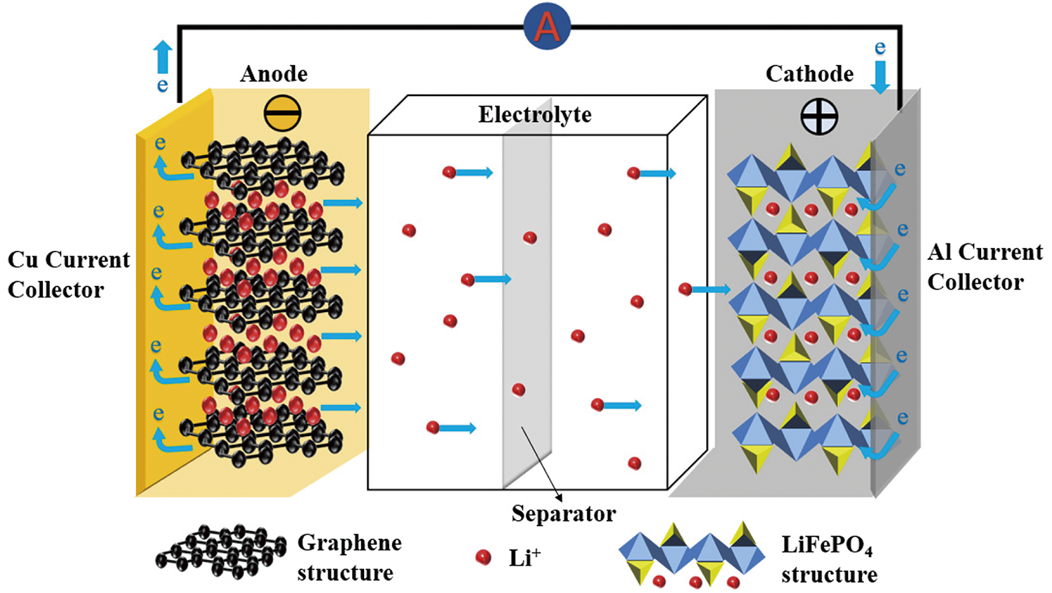
Figure 1: A schematic diagram of the internal structure of a LiFePO4 battery

According to different viewpoints, SOH can be defined in various forms [39]. It is common to define SOH in terms of internal resistance R or remaining capacity C. The SOH as defined by the internal resistance is presented in the following formula, which represents the proportion of the current internal ohmic resistance Rt to the initial internal ohmic resistance of a new battery R0:

SOHt=RtR0(1)

Similarly, the SOH as defined by the capacity represents the ratio of the remaining capacity Ct to the nominal capacity C0:

SOHt=CtC0(2)

The capacity C0, which is specified by the battery manufacturer for a particular battery type, is analogous to the initial capacity Ct0 of a new battery at the Beginning of Life (BOL). However, there may be differences between them due to manufacturing process deviations. Subsequently, we will mainly focus on the SOH defined based on capacity, as it reflects the energy capacity and range of the battery. In contrast, the SOH defined by internal resistance reflects the power capabilities.

3.2 Battery Data Set

As shown in Fig. 2, an experimental platform has been established to investigate the characteristics of a battery. The data set was obtained by the aging test system using the life experiment of 179 Ah CBOMHW3NA battery at room temperature of 25°C. The platform includes: (1) Battery Test System: This system enables batteries to undergo repetitive charge and discharge processes, providing essential insights into their capacity and performance under real-world conditions. (2) Grading Machine: The grading machine helps categorize batteries based on their performance metrics after cycling. It is an essential part of the system that assesses each battery’s capacity, ensuring quality and reliability in subsequent applications. (3) Data Acquisition Instrument: The computer setup linked to the test system functions as a data acquisition tool. It monitors and records critical parameters, such as current, voltage, and temperature, from the batteries during the test cycles. This real-time data collection allows for accurate tracking of the battery’s SOH. This comprehensive setup supports a detailed analysis of battery performance by precisely capturing and evaluating the necessary electrical and thermal data during testing.

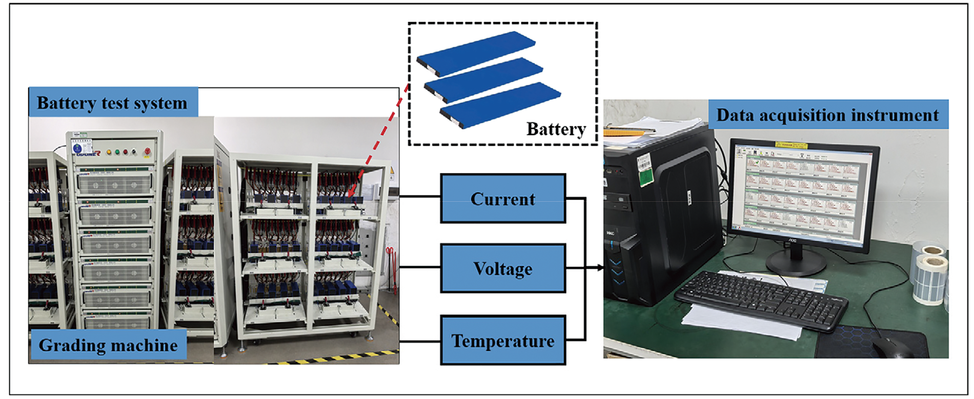
Figure 2: Battery cycle aging test platform

In order to simulate daily use, the following experimental process was set up in this study: First, the LIB was charged to 3.65 V at a constant current of 50 A, and then continued to charge in a constant voltage mode until the cut-off current reached 3.6 A, and then kept charged to full capacity. The LIB is then discharged with a constant current until the voltage drops to 2.3 V. Repeat the above cycle until the LIB’s SOH drops to 80%.

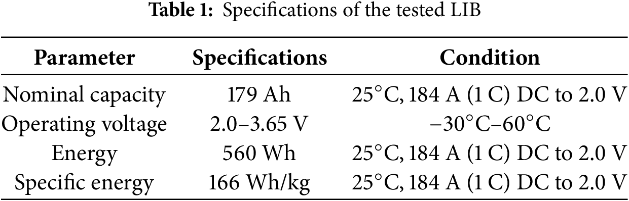
The nominal specifications of the tested LIB are shown in Table 1. These parameters include capacity, voltage range, energy, operating temperature range, etc., which is an important basis for experimental design and result analysis. LIB parameters will be different under different conditions. This experiment adopts the condition of 25°C and takes the capacity after 184 A constant current discharging (DC) to 2 V as the standard value.

3.3 Feature Extraction

The SOH of LIBs is affected by many factors, including the number of cycles, temperature, charge and discharge rate, and storage conditions. These factors are complex and diverse, there is no direct coupling relationship, and SOH cannot be directly measured, so it is necessary to extract HIs that are correlated with SOH from the charge and discharge curve of LIBs, and estimate the SOH of LIBs based on HI.

An extensive review of the literature reveals that most studies on SOH estimation have selected features related to voltage, current, and temperature, as these physical quantities are closely linked to the internal electrochemical reactions and aging mechanisms of batteries [40]. Based on this understanding, we conducted a detailed analysis of the voltage and current curves during the charge-discharge process of LIBs.

The voltage and current curves during charge and discharge across four different cycles—namely the 1st, 54th, 116th, and 170th cycles—are illustrated in Fig. 3. As the number of cycles increases, noticeable deviations appear in the voltage and current curves, which indicates progressive battery degradation. In the early stages of cycling, such as in the 1st cycle, the voltage and current curves exhibit relatively stable patterns during both charge and discharge phases. However, as the cycle number increases to the 54th, 116th, and 170th cycles, noticeable changes occur.

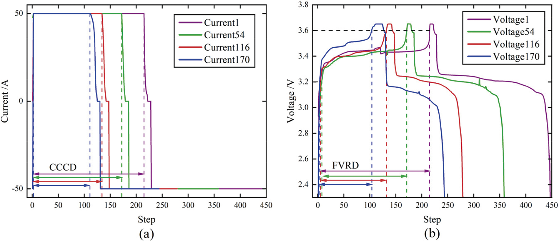
Figure 3: Charge and discharge process curve of LIB (a) Voltage curve (b) Current curve

In the voltage curves, the Constant Current (CC) charging stage shows a gradual reduction in duration, while the Constant Voltage (CV) stage lengthens as the battery ages. This suggests that the battery reaches the cut-off voltage more quickly, but it takes longer to charge to full capacity as its internal resistance increases. Similarly, during discharge, the voltage drop becomes steeper, particularly in the later cycles, implying a faster depletion of energy. The current curves further demonstrate this degradation, with the current during the CV phase dropping more rapidly in the later cycles. Additionally, the discharge current also decreases more sharply, indicating a reduction in the battery’s ability to sustain current as it ages.

The deviations in both voltage and current curves across different cycles reflect the evolution of the battery’s internal characteristics, including capacity fade and increased internal resistance, which are typical signs of SOH degradation over time.

Based on these voltage-current curves and empirical analysis, six HI in charge and discharge process are initially extracted, which are closely related to SOH:

HI1: Fixed Voltage Rise Duration (FVRD) refers to the time required for the battery to rise from one fixed voltage to another during the charging process. In this paper, the time used for the battery to rise from 3.2 to 3.6 V is selected. The time reflects the charging efficiency and internal resistance changes of the battery in this voltage range, and the increase of internal resistance will lead to the extension of the voltage rise time, thus reflecting the aging degree of the battery.

HI2: CC Charging Duration (CCCD) refers to the time required by the battery during the CC phase of the charging process. As the battery ages, the duration of the CC charging phase changes, usually due to increased internal resistance of the battery and reduced charging efficiency.

HI3: Discharge Efficiency (DE) refers to the ratio of the effective energy that a battery can release during discharge to its nominal capacity. The reduction of discharge efficiency usually indicates the attenuation of battery capacity and the increase of internal loss, which is an important indicator to measure the health status of the battery.

HI4: Maximum Temperature (MT) indicates the highest temperature of a battery during charging. This metric may be limited due to the low accuracy of the temperature sensor, but can still provide basic information about the thermal management performance of the battery. Battery aging may lead to an increase in maximum temperature, reflecting a decrease in heat dissipation performance.

HI5: Time to Peak Temperature (TPT) refers to the time required for a battery to reach its highest temperature during charging. This indicator reflects the thermal efficiency and heat dissipation performance of the battery during the charging process, and the aging battery may reach the maximum temperature faster.

HI6: Final Temperature (FT) refers to the temperature of the battery at the end of the charging process. This indicator provides information on the thermal management performance of the battery at the end of charge, and aging batteries may exhibit higher temperatures at the end of charge, reflecting an increase in their internal impedance and a decrease in thermal stability.

These HI’s provide an important input to SOH estimates, and with further correlation analysis, these HI’s can help us more accurately predict battery health.

4  Methodology

4.1 Pearson Correlation Analysis

PCA was used to analyze the correlation between HI and SOH. Pearson Correlation Coefficient (PCC) is a statistical index that measures the strength and direction of the linear relationship between two variables. Its value ranges from −1 to 1, where 1 means completely positive correlation, −1 means completely negative correlation, and 0 means no correlation. The PCC is calculated as follows:

r=∑(xi−x¯)(yi−y¯)∑(xi−x¯)2(yi−y¯)2(3)

where r represents the PCC, xi and yi are the sample values of the two variables. In addition, x¯ and y¯ are the mean values of the variables x and y, respectively.

By standardizing the covariance of two variables, PCC obtains a dimensionless correlation coefficient, which can effectively measure the linear relationship between two variables. This coefficient has important applications in data analysis and feature selection, especially in evaluating correlations and dependencies between variables [41].

4.2 Gaussian Process Regression

GPR is a probabilistic framework based non-parametric regression technique that is widely used in machine learning and statistical modeling. GPR provides a powerful way to estimate the behavior of unknown functions by assuming that data can be generated from a multidimensional Gaussian distribution covering an infinite number of data points. The core advantage is that it can provide not only the forecast itself, but also the uncertainty of the forecast, that is, the confidence interval of the forecast.

In the GPR model, each data point is treated as a random variable, and the joint distribution of all data points constitutes a Gaussian process. The model is defined by a mean function and a covariance function, as shown in Eqs. (4)–(6):

f(x)=GP[m(x),k(x,x′)](4)

m(x)=E[f(x)](5)

k(x,x′)=E{[f(x)−m(x)][f(x′)−m(x′)T]}(6)

In the formula, m(x) is the mean value function, which can usually be set to zero, that is, m(x)=0; k(x,x′) is the covariance function or kernel function, which is the key in the modeling process and describes the correlation between any two data points. Here, E(⋅) represents expectation and f(x) is an implementation of the Gaussian process. The learning process of GPR involves optimizing the parameters of the kernel function, as well as maximizing the logarithmic likelihood function of the data, thereby learning the intrinsic structure and pattern of the data.

The core principle of GPR prediction is that you are given a training data set X={x1,x2,⋯,xn} and a corresponding observation value Y={y1,y2,⋯,yn}. Suppose there is a relationship Y=f(x) + ε between the function f(x) and the observed value, where ε is the observed noise, which is usually assumed to be Gaussian noise, satisfying Eq. (7):

ε∼N (0,σn2)(7)

Given a new set of input points X∗, the output value Y of the training point and the output value f∗ of the prediction point follow a Gaussian distribution according to the nature of the Gaussian process:

(Yf∗)∼N (0,(K (X,X)+σn2IK (X,X∗)K (X∗,X)K (X∗,X∗)))(8)

where K (X,X) is the covariance matrix between training points, K (X,X∗) is the covariance matrix between training points and prediction points, σn2I is the noise, and I is the identity matrix.

Finally, given the training data, the conditional distribution of the output value f∗ at the predicted point X∗ is a Gaussian distribution, whose mean and variance are:

μ(X∗)=K (X∗,X)[K (X,X)+σn2I]−1Y(9)

σ2(X∗)=K (X∗,X)−K (X∗,X)[K (X,X)+σn2I]−1K (X,X∗)(10)

The 95% confidence interval for the output of the Gaussian process regression above is:

[μ(X∗)−1.96×σ2(X∗),μ(X∗)+1.96×σ2(X∗)](11)

4.3 Noisy Input Gaussian Process

GPR is a powerful non-parametric statistical model for performing regression and classification tasks. However, the SOH estimation of LIB is a complex nonlinear multi-input/output fitting problem, and the traditional GPR is very sensitive to noise, which affects the accuracy of the estimation. In order to solve this problem, NIGP is proposed, which can effectively deal with the noisy input data and improve the robustness and prediction accuracy of the model. The advantage of the NIGP model is that it is not only suitable for noisy input data, but also provides an estimate of the prediction uncertainty. It modifies the variance estimate of the output by estimating the impact of input noise, so that the output of the model can be predicted more accurately, especially when the input data is uncertain [42].

Suppose our training set is X={xi}i=1n and Y={yi}i=1n, where xi is the input feature and yi is the corresponding output. The input noise model is introduced, assuming that xi is affected by Gaussian noise ε, i.e., xi∼N(x~i,Σx), where x~i is the observed input and Σx is the covariance matrix of the noise.

In NIGP, the revised covariance matrix is:

K (X,Z)=K (X,X)+Σx(12)

where X represents the input feature matrix of the training data set, with each row representing a sample and each column representing a feature; Z represents a new test input point (or a new prediction point); K (X,X) is the covariance matrix on training data set X, K (Z,X) is the covariance matrix between test point Z and training data set X, and K (Z,Z) is the covariance matrix of test point Z itself, all of which are calculated by kernel function; Σx is the noise covariance matrix in the input data X.

The final predicted distribution is:

p(y~|Z,X,Y)=N(y~|μ(Z),σ2(Z))(13)

μ(Z)=K (Z,X)[K (X,X)+σn2I]−1Y(14)

σ2(Z)=K (Z,Z)−K (Z,X)[K (X,X)+σn2I]−1K (X,Z)(15)

where σn2 is the variance of the observed noise, μ(Z) is the predicted mean at test point Z, and σ2(Z) is the predicted variance at test point Z.

In the NIGP model, the noise in the input data is processed by modifying the covariance matrix K (X,Z). This correction takes into account the effect of noise on the similarity between the input data points, which more accurately reflects the true distribution of the data. When we calculate the prediction of the test point Z, the effect of noise is reflected not only by the modification of the covariance matrix, but also by the additional terms in the prediction variance σ2(Z). This additional variance correction allows the model to provide reasonable confidence intervals in the presence of input noise, improving the robustness of the model under uncertain conditions. In this way, NIGP model can effectively deal with the noise in the input data, and consider the influence of noise on the covariance matrix in the prediction process, and finally get a more robust prediction result.

4.4 Beluga Whale Optimized Gaussian Process Regression Model

GPR has been widely used in many fields, and its performance highly depends on the reasonable settings of parameters such as length scale and covariance. Traditional parameter determination methods often have limitations, while metaheuristic algorithms like BWO algorithm provide a new approach to solve this problem. BWO algorithm was proposed by Zhong et al. [43], a scholar from Dalian University of Technology, in 2022, which is an evolutionary algorithm inspired by the swimming, hunting, and survival behaviors of Beluga whales. The following will elaborate in detail on how the BWO algorithm optimizes the length scale and covariance in GPR.

The covariance function adopts the squared exponential covariance function, which is defined as:

k(xi,xj)=σ2exp⁡(−12l2∑d=1D(xi,d−xj,d)2)(16)

where xi and xj are the input data, σ2 is the signal variance, l is the length scale, and D is the dimension of the input data. The optimization objective is to find the optimal values of l and σ2. The log marginal likelihood is selected as the indicator, aiming to maximize the log marginal likelihood. The formula is as follows:

ln⁡p(y|X,l,σ2)=−12yTK−1y−12ln⁡|K|−n2ln⁡(2π)(17)

where y is the vector of the observed target values, X is the input data matrix, K is the covariance matrix, and n is the number of data points.

The BWO algorithm needs to go through the initialization, exploration, exploitation, and whale fall stages. In the initialization stage of the BWO algorithm, the parameters related to the length scale l and the signal variance σ2 are regarded as variables to be optimized and form the position vector of the beluga whale individual. For example, for the i-th beluga whale, its position is represented as Xi=[li,σi2]. Randomly initialize the positions of all beluga whales within the search space, and simultaneously set the population size n and the maximum number of iterations Tmax.

The balance factor Bf=B0(1−T/2Tmax) determines whether the beluga whale enters the exploration stage or the exploitation stage. Where T is the current iteration number, and B0 randomly takes values within 0 to 1 in each iteration. When Bf>0.5, the beluga whale enters the exploration stage, and the formula is as follows:

Xi,jT+1=Xi,pjT+(Xr,p1T−Xi,pjT)(1+r1)ei^(2πr2)(18)

ei^(2πr2)=cos⁡(2πr2)+i^sin⁡(2πr2),i^=−1(19)

where Xi,jT+1 is the new position of the i-th beluga whale in the j-th dimension (j=1 corresponds to l, j=2 corresponds to σ2), pj is a randomly selected dimension from the two dimensions, Xi,pjT is the current position of the i-th beluga whale in the pj dimension, Xr,p1T is the current position of the randomly selected r-th beluga whale, and r1 and r2 are random numbers within (0,1).

When Bf≤0.5, the beluga whale enters the exploitation stage, and the formula for position update is as follows:

XiT+1=r3XbestT−r4XiT+C1⋅A(XrT−XiT)(20)

where XiT and XrT are the current positions of the i-th and randomly selected beluga whales, respectively, XbestT is the best position in the current population, and r3 and r4 are random numbers between (0,1). C1=2r4(1−T/Tmax) is the random jump intensity, and A is the acceptance criterion term related to simulated annealing, and its calculation method is as follows:

Calculate the log marginal likelihood L(XiT) corresponding to the current position XiT and the log marginal likelihood L(XiT+1) corresponding to the new position XiT+1, calculate the difference ΔL=L(XiT+1)−L(XiT), then A=exp⁡(−ΔL/T). If the random number r is less than A, the new position is accepted; otherwise, the current position is retained.

In each iteration, calculate the whale fall probability according to the formula Wf=0.1−0.05T/Tmax. Some beluga whales may die due to whale fall and fall into the deep sea, and the formula for position update is:

XiT+1=r5XiT−r6XrT+r7Xstep(21)

where r5, r6 and r7 are random numbers between 0 and 1, and Xstep is the whale fall step length, and its calculation formula is Xstep=(ub−lb)exp⁡(−C2T/Tmax) (where C2=2Wf×n, ub and lb are the reasonable upper and lower boundaries of l and σ2, respectively). The step length is affected by the variable boundaries, the number of iterations and the maximum number of iterations to ensure that the updated l and σ2 are still within a reasonable range.

After updating the position of the beluga whale each time, use the updated parameter values to calculate the log marginal likelihood in the GPR algorithm as the fitness value. Sort the beluga whales in the population according to the fitness value and find the currently optimal beluga whale. Check the termination condition. If the current iteration number is less than the maximum iteration number, continue to the next iteration and repeat the exploration, exploitation and whale fall stages; otherwise, stop the iteration and output the optimal values of l and σ2 as the optimized parameters of the GPR algorithm. The parameter optimization process of GPR by BWO is illustrated in Fig. 4.

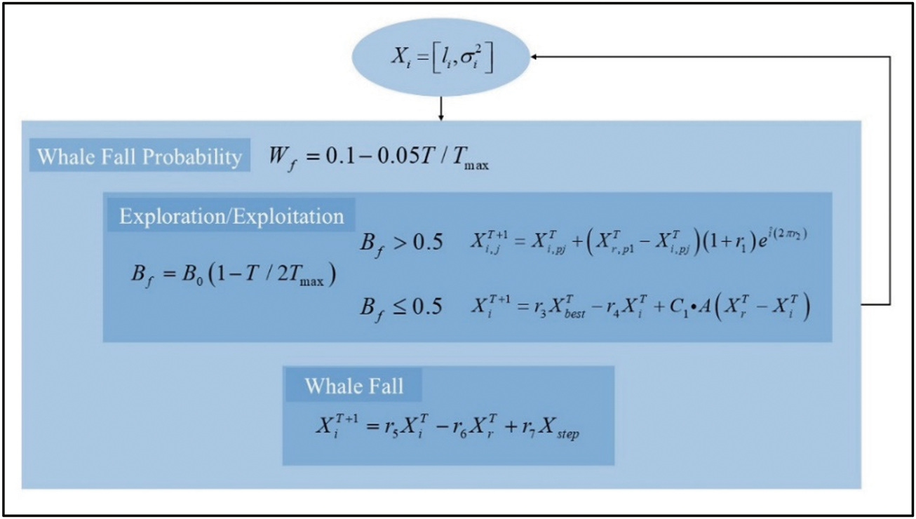
Figure 4: The flowchart of GPR optimization based on BWO

Through the above optimization process of the length scale and covariance in GPR by the BWO algorithm, it is possible to search for a better combination of parameters in the complex parameter space, thereby improving the performance of the GPR model and enabling it to make more accurate predictions and modeling in practical applications. Meanwhile, the adaptive characteristics and global search ability of the BWO algorithm help overcome the problem that traditional optimization methods are prone to falling into local optima, providing an effective solution for the parameter optimization of the GPR algorithm.

4.5 BWO-GPR and NIGP Stacked Model

The flowchart of the proposed BGNSM for lithium-ion battery SOH estimation is presented in Fig. 5. The framework is divided into three primary stages: Data Acquisition, Modeling Process, and Error Analysis each designed to systematically enhance the accuracy and robustness of the estimation process.

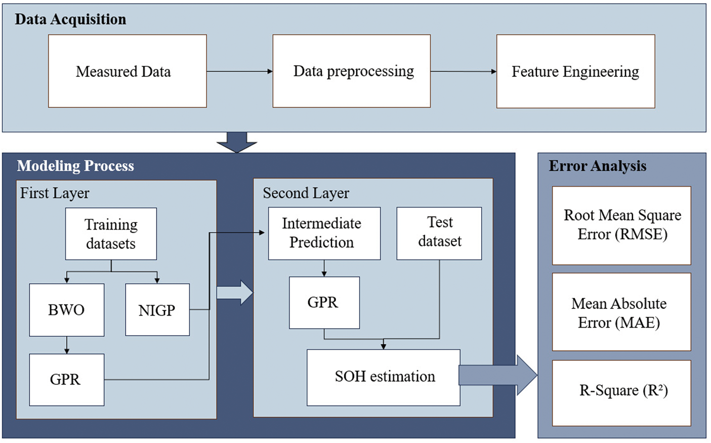
Figure 5: Schematic of the BGNSM estimation method

Firstly, in the Data Acquisition phase, historical operating data, including voltage, current, temperature, and charge/discharge cycles, is gathered. Afterward, the data undergoes preprocessing to ensure its quality—this involves data cleaning, normalization, and feature engineering. The feature engineering process focuses on extracting key attributes most relevant to SOH estimation.

Secondly, the Modeling Process is split into two layers:

1. In the First Layer, training datasets are utilized to simultaneously train the BWO-optimized GPR model and the NIGP model. BWO is initialized to optimize GPR hyperparameters, allowing for a comprehensive exploration of the hyperparameter space and preventing the model from falling into local optima. NIGP is also trained in parallel to manage noise in the input data. The outputs from both the BWO-GPR and NIGP models are then used to generate intermediate predictions.

2. In the Second Layer, these intermediate predictions serve as inputs to a second GPR model. This second-layer GPR model combines the outputs from both BWO-GPR and NIGP, refining the predictions and delivering the final SOH estimation.

Finally, in the Error Analysis phase, the model’s performance is evaluated using several key metrics: RMSE, MAE, and R2 value. These metrics provide a comprehensive assessment of the model’s accuracy, stability, and robustness, ensuring that it meets the necessary requirements for reliable SOH estimation.

By now, the combined BWO-GPR and NIGP estimation framework has been developed. It can be iterated to achieve precise aging state estimation of batteries.

5  Results and Discussion

5.1 Screening of HI

In Section 3.3, six HIs related to SOH are initially selected according to the charge and discharge curve characteristics of LIB. Fig. 6 shows the change curve of each health factor, and these subgraphs show the evolution of different factors during the LIB cycle. By analyzing the trends of these health factors, we can identify and pick out the characteristics that are highly correlated with battery capacity for the prediction of battery SOH.

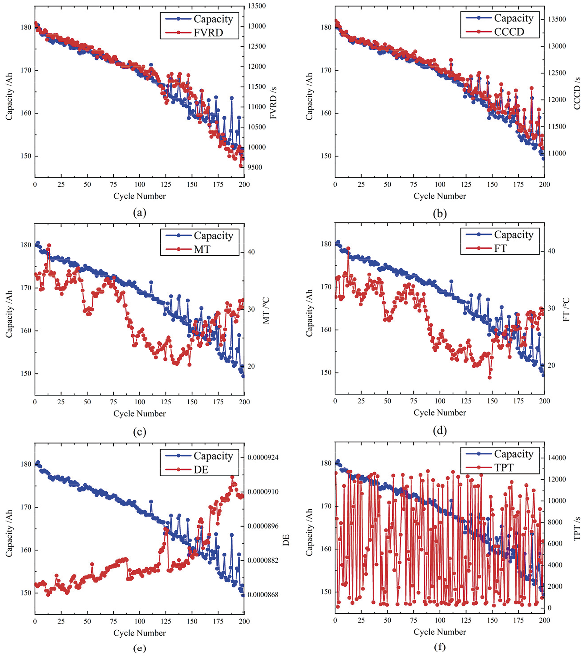
Figure 6: Change curves of His (a) FVRD (b) CCCD (c) MT (d) FT (e) DE (f) TPT

As shown in Fig. 6, the capacity gradually decreases with the increase of the number of cycles, reflecting the capacity decay and aging process of the battery. Among them, the change trend of FVRD shows that with the increase of the number of cycles, FVRD gradually increases, which indicates that the internal resistance of the battery is constantly increasing, resulting in a decrease in charging efficiency. FVRD shows a high correlation with capacity decline and is an important indicator for evaluating battery aging. DE gradually decreases during the cycle, and the trend is highly consistent with the attenuation of capacity, which means that the energy loss of the battery during the charge and discharge process gradually increases, reflecting the gradual degradation of the battery performance. The trend of CCCD also shows that CCCD gradually increases with the increase of the number of cycles, which is highly correlated with the decrease of capacity, indicating that the charging efficiency of the constant current stage decreases with aging. In contrast, although features such as MT, TPT, and FT reflect the thermal management and energy input and output of the battery, their correlation with capacity is relatively low. TPT, in particular, has an extremely low correlation with capacity, suggesting that this feature contributes less to the prediction of battery capacity. Therefore, FVRD, DE and CCCD, which are highly correlated with capacity, are given priority in feature selection.

In order to ensure the accuracy of data analysis, this study further uses PCC to quantitatively analyze the correlation between various health factors and battery capacity. The data in Table 2 show that there are significant differences in the correlation between different health factors and battery capacity.

For example, the correlation coefficient between FVRD and capacity is 0.956, indicating a very high positive correlation between the two variables. The correlation coefficient of CCCD is even higher, reaching 0.999, which is an almost perfect positive correlation, indicating that CCCD can almost fully reflect changes in battery capacity and is an extremely critical feature in predicting battery SOH. The PCC of DE is −0.884, showing a high negative correlation, indicating that DE decreases with the reduction of battery capacity, and is an important negative correlation factor for predicting battery aging. In contrast, the correlation coefficient of MT is 0.585, showing a moderate degree of positive correlation, indicating that although it can reflect certain battery thermal management performance, it is poor in predicting capacity. The correlation coefficient of TPT is only 0.06, which is almost no correlation, indicating that its contribution to capacity prediction is extremely limited. The correlation coefficient of FT is 0.597, showing a moderately positive correlation, but still less important than FVRD, CCCD, and DE.

To sum up, FVRD, CCCD and DE are selected as the features with the highest correlation with volume through qualitative analysis of the graphs and quantitative analysis of PCCs. These features can not only effectively capture changes in battery performance, but also reflect important trends in the aging process of batteries. With the increase of the number of battery cycles, the increase of FVRD and CCCD indicates that the internal impedance of the battery rises, while the decrease of DE reflects the attenuation of the battery capacity. These characteristics will be applied to the subsequent LIB SOH prediction model to improve the accuracy and reliability of the prediction.

5.2 Result of SOH Estimation by BGNSM Model

The first 50% of the collected data is used for model training, and the remaining 50% is used for model validation. From Fig. 7, it can be seen that the proposed BGNSM model has high accuracy in predicting SOH in LIB. The BGNSM model’s predicted SOH curve is highly consistent with the actual SOH curve, and the error between the predicted and actual values is maintained within 1%. Especially in the early and middle stages of battery power decline, the predicted values of the model are almost completely consistent with the actual values, indicating that the model still has high accuracy in capturing the trend of battery power decline in small sample situations. Although the overall prediction error remains at a low level, there is a slight increase in prediction error at certain specific time points or intervals where battery state changes are more drastic. The increase in these errors may be related to factors such as data noise, improper adjustment of model parameters, or incomplete capture of complex reaction mechanisms within the battery.

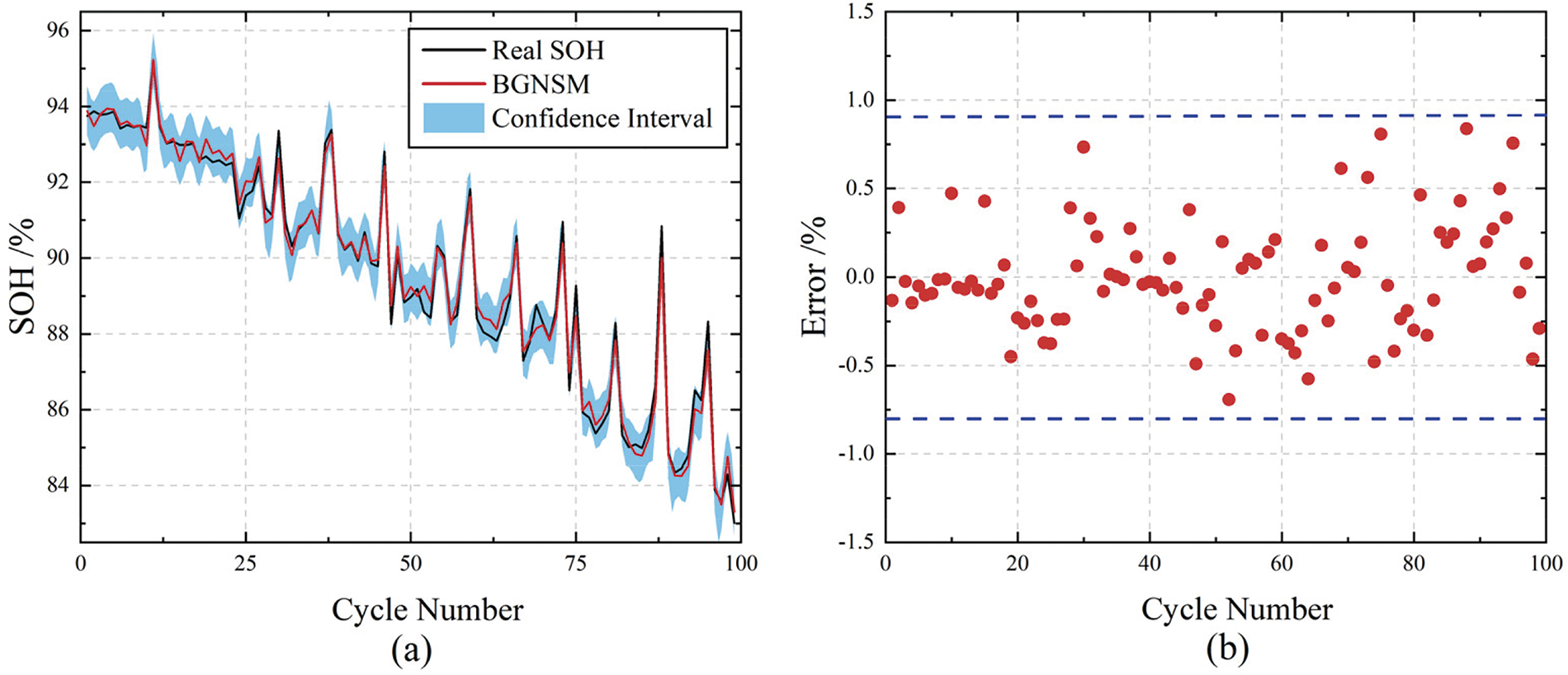
Figure 7: SOH estimation of LIB by BGNSM model (a) SOH estimation for CBOMHW3NA (b) Estimation error of SOH

In addition, the shaded areas in the Fig. 7 represent the confidence intervals of the predicted results. The narrow confidence interval indicates that the BGNSM model can not only accurately predict the SOH value of the battery, but also demonstrate good control ability in predicting uncertainty. This is particularly important because in practical applications, the uncertainty of predictions directly affects the decision-making process of BMS. The narrow confidence interval further proves the robustness and reliability of the model. In some extreme cases, such as rapid battery aging or severe failures, the confidence interval may expand, reflecting an increase in predictive uncertainty of the model in these situations. Therefore, in practical applications, we need to make a comprehensive judgment by combining confidence intervals and predicted values to more accurately evaluate the SOH state of the battery.

5.3 Estimation Results for Different Models

In order to objectively evaluate the performance of the proposed model, the current popular evaluation indexes were selected, including RMSE, MAE and R2. These indexes can comprehensively measure the prediction accuracy and stability of the model.

RMSE reflects the average error between the predicted value and the true value. The smaller the value, the higher the prediction accuracy. The calculation formula is as follows:

RMSE=1n∑i=1n(Xi−X^i)2(22)

MAE reflects the average absolute error between the predicted value and the true value. A smaller value means that the model prediction is closer to the reality. The calculation formula is as follows:

MAE=1n∑i=1n|Xi−X^i|2(23)

R2 measures the proportion of the total variation of the explanatory variables of the model. The closer the value is to 1, the stronger the explanatory power of the model. The calculation formula is as follows:

R2=1−∑i=1n(Xi−X^i)2∑i=1n(Xi−X¯)2(24)

In the above formula, Xi is the ith actual value, X^i is the ith predicted value, and X¯ is the average of the actual value.

Through the calculation of the above evaluation indexes, the prediction performance of the model can be evaluated comprehensively to ensure its effectiveness and reliability in practical application.

In Fig. 8a, the SOH estimation results using NIGP show significantly higher accuracy compared to traditional GPR, particularly as the cycle number increases. This trend is further highlighted in the error plot in Fig. 8b, where NIGP consistently demonstrates a smaller error margin, especially in the later stages of battery cycling. The key advantage of NIGP lies in its robust noise-handling capabilities, allowing it to maintain precise estimations across various cycles. The performance metrics provided in the Table 3 further substantiate this. NIGP achieves an RMSE of 0.526%, an MAE of 0.378%, and an R2 of 0.97, clearly outperforming GPR in all respects. These lower RMSE and MAE values indicate that NIGP provides more accurate predictions with less deviation, while the higher R2 value shows that NIGP captures more of the variance in the data, leading to a better model fit. Notably, NIGP also demonstrates better computational efficiency with a time cost of 8.5 s, significantly lower than GPR’s 15.2 s, indicating its advantage in both accuracy and efficiency. Collectively, these results emphasize that NIGP’s ability to handle input noise is critical to providing more reliable and robust SOH estimations across a wide range of battery cycles, outperforming traditional GPR in both accuracy and consistency.

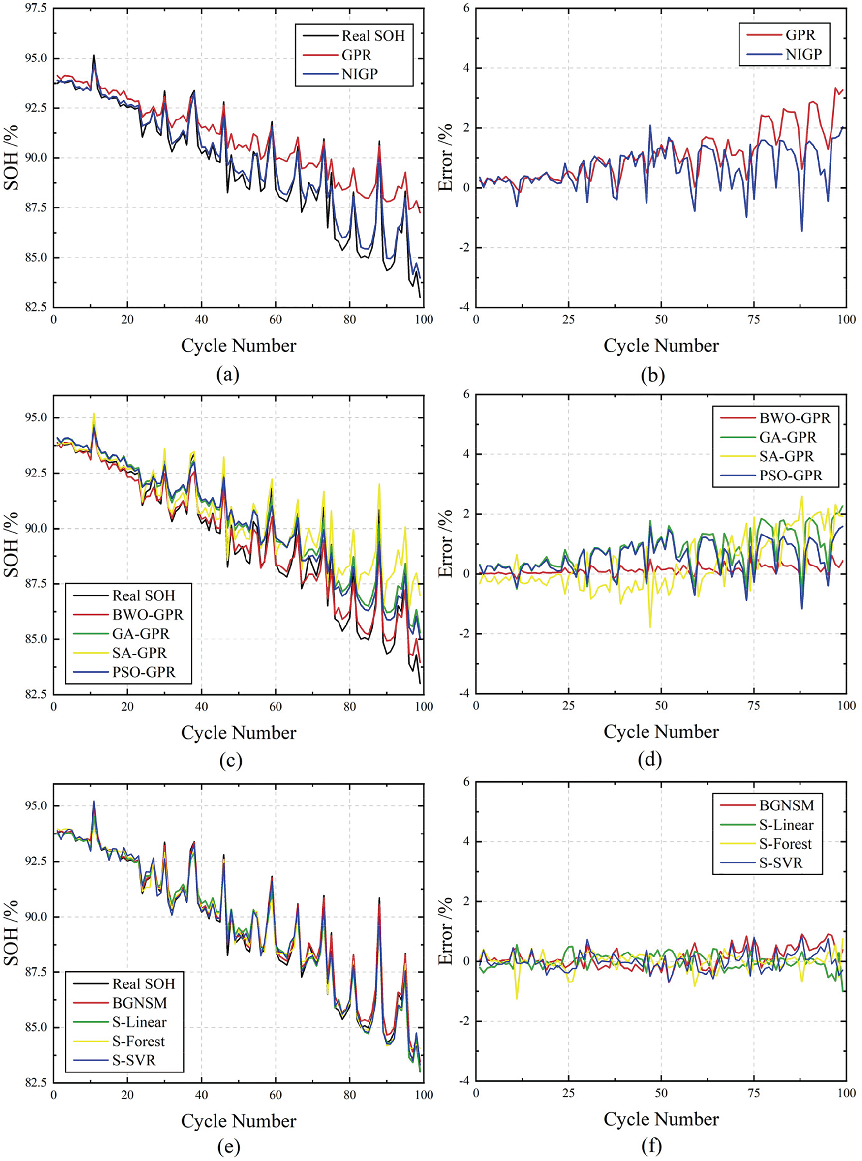
Figure 8: Results of SOH estimation by different models (a,c,e) Results of SOH estimation. (b,d,f) Estimation error between Estimation and Real SOH

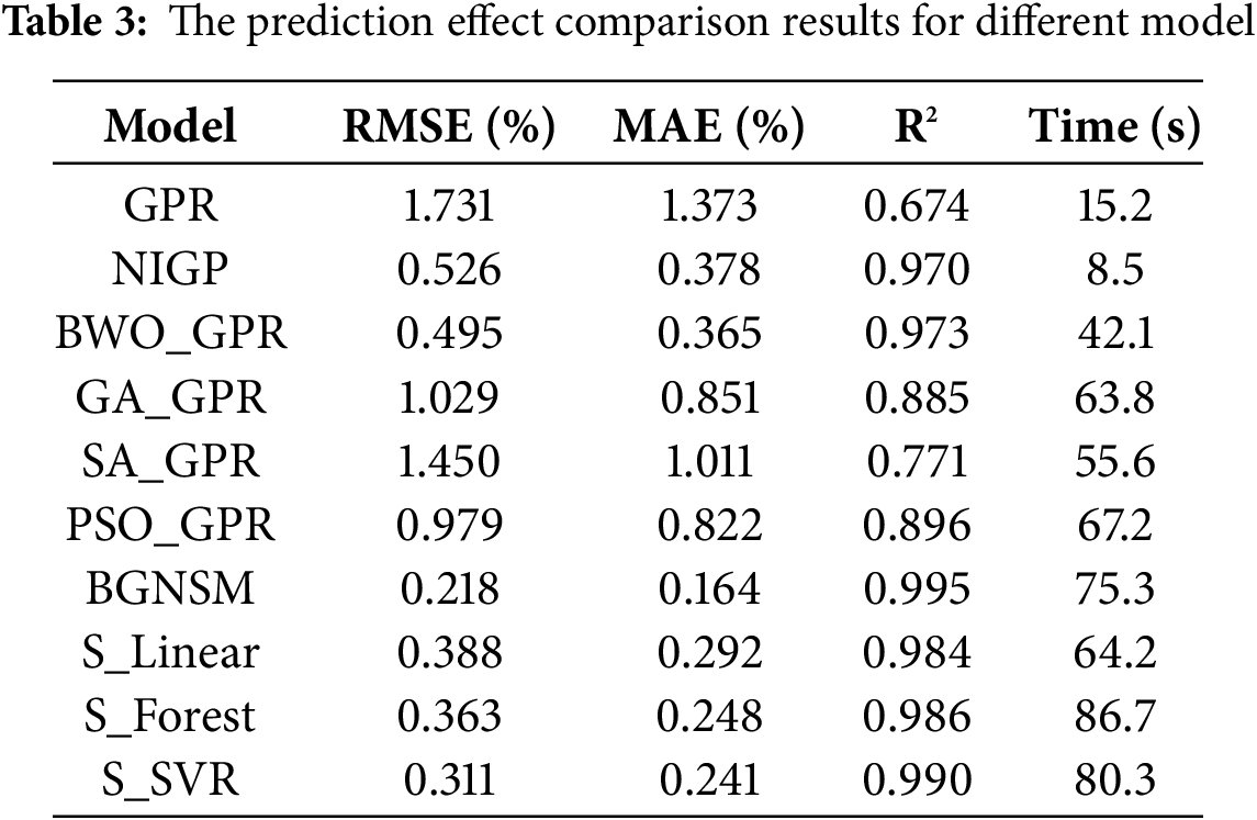
Fig. 8c presents the SOH estimates obtained through four distinct optimization methods, namely BWO, Genetic Algorithms (GA), Simulated Annealing (SA), and Particle Swarm Optimization (PSO). Evidently, the BWO-GPR approach yields notably smoother and more precise SOH estimations, exhibiting fewer fluctuations when compared to the other techniques. As depicted in Fig. 8d, the error margins associated with BWO-GPR remain consistently lower throughout all cycles. Moreover, Table 3 further accentuates the superiority of BWO-GPR, which registers an RMSE of 0.495%, an MAE of 0.365%, and an R2 of 0.973, outperforming GA-GPR and PSO-GPR. This unequivocally showcases that BWO offers a more efficacious and accurate means of hyperparameter optimization in contrast to GA, SA, and PSO. In addition, BWO takes significantly less time to optimize GPR than GA, SA and PSO, indicating that BWO is more efficient in optimizing GPR algorithm.

In Fig. 8e, the SOH estimation results of the BGNSM are presented, showcasing the advantages of this stacked approach. Instead of relying on individual models, the outputs from both NIGP and BWO-GPR are integrated to form a more robust prediction framework. This combination allows for the noise-handling capability of NIGP to be complemented by the optimization strength of BWO-GPR. The error plot in Fig. 8f demonstrates that the stacked model significantly reduces prediction errors compared to using either model alone. This improvement is further validated by the performance metrics in Table 3, where the combined model achieves the lowest RMSE of 0.218%, MAE of 0.164%, and an exceptionally high R2 of 0.995. These results highlight the effectiveness of this integrated approach, which leverages the strengths of both NIGP and BWO-GPR to produce more accurate and consistent SOH predictions across all battery cycles. This synergy between the models leads to a more reliable estimation process, outperforming single-model approaches. To further validate the contribution of each component in the stacked integration model, an ablation study was conducted.

This involved systematically removing one model from the stack and re-evaluating the performance. When NIGP was removed and only BWO-GPR was used, the model’s RMSE increased to 0.495%, and its R2 dropped to 0.973, showing a decline in predictive accuracy and model fit. Similarly, when BWO-GPR was removed and only NIGP was used, the RMSE rose to 0.526% and R2 decreased to 0.97, indicating that the optimization strength of BWO-GPR is crucial for reducing error margins and improving overall prediction accuracy. The results of this ablation study demonstrate that both NIGP’s noise-handling capabilities and BWO-GPR’s optimization efficiency are essential components of the model’s success. Removing either significantly degrades performance, highlighting the importance of integrating both models in the BGNSM framework.

Finally, within the second-level stacking procedure, employing GPR as the central model for the stacking layer generates more favorable outcomes compared to alternative models like Linear Regression (S-Linear), Random Forest (S-Forest), or Support Vector Regression (S-SVR). The error plot illustrated in Fig. 8f distinctly reveals that the BGNSM consistently outshines the other stacked models throughout all cycles. This is further corroborated by the data presented in Table 3: although models such as S-Linear and S-Forest attain a reasonable level of accuracy, the BGNSM’s R2 value of 0.995 substantially exceeds theirs. In terms of running time, although BGNSM is slightly slower than S-Linear, its accuracy is much higher than S-Linear, and BGNSM is more cost-effective. These results firmly validate that when GPR is utilized as the ultimate model in the second-layer stacking, it delivers the most accurate and reliable SOH predictions.

5.4 Comparison of Model Performance with Different Stacking Layers

To investigate the impact of multiple stacking models on the accuracy and computational efficiency of SOH estimation, we evaluated the performance of stacking models one, two, three, ten, and fifty times. The aim of this analysis is to assess whether additional stacked layers offer meaningful accuracy improvements or merely increase computational complexity without providing additional benefits.

As illustrated in Fig. 9, stacking the model once strikes an optimal balance between accuracy and computation time. The RMSE and MAE values for the one-time stacked model are 0.218% and 0.164%, respectively, with an R2 of 0.995 and a calculation speed of 17.725 s. The results demonstrate that this method boasts high accuracy, low computational cost, and is thus an efficient approach for SOH estimation.

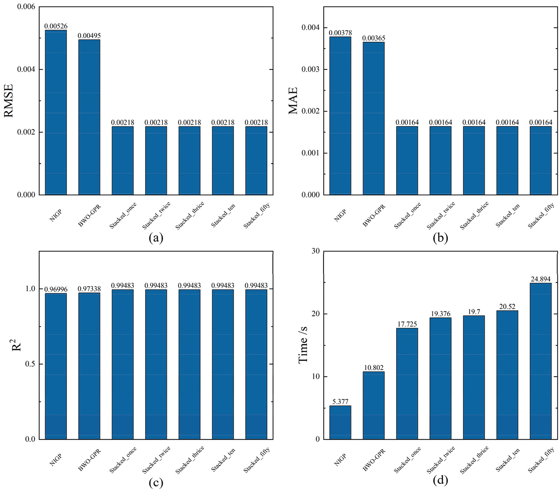
Figure 9: Error of SOH estimation with Different Stacking Layers (a) RMSE of SOH estimation with different stacking layers (b) MAE of SOH estimation with different stacking layers (c) R2 of SOH estimation with different stacking layers (d) Time of SOH estimation with different stacking layers

However, when the model was stacked twice or more, the results indicated no improvement in performance. Instead, the computation time nearly doubled to 24.894 s. This suggests that while there is a marginal gain in accuracy, the increase in complexity and computational cost is disproportionate. Further stacking to multiple layers can lead to even worse results. These findings suggest that stacking more than once incurs unnecessary computational overhead without significantly enhancing accuracy. Therefore, stacking once strikes an optimal balance between model accuracy and processing time, while additional stacking layers can lead to diminishing returns.

5.5 Comparison of Prediction Results for Different Proportions of Training Sets

In this section, by systematically adjusting the proportion of training sets, using 10%, 25%, 50% and 75% data sets as training sets, the performance ability of the model under different data sizes was deeply explored, especially its processing ability for small sample data. Experimental error results are shown in Table 4, and prediction curve results and confidence intervals are shown in Fig. 10.

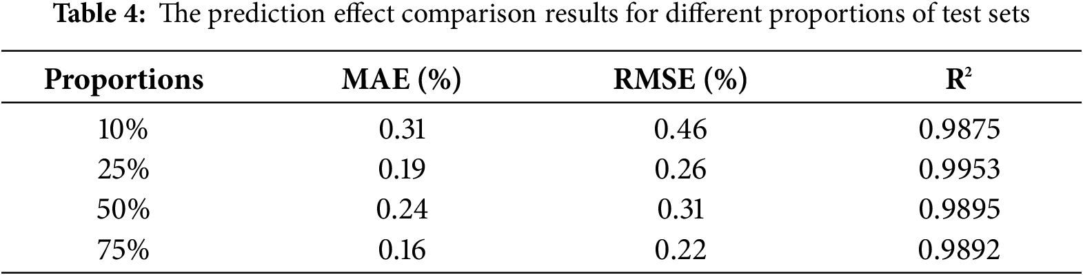
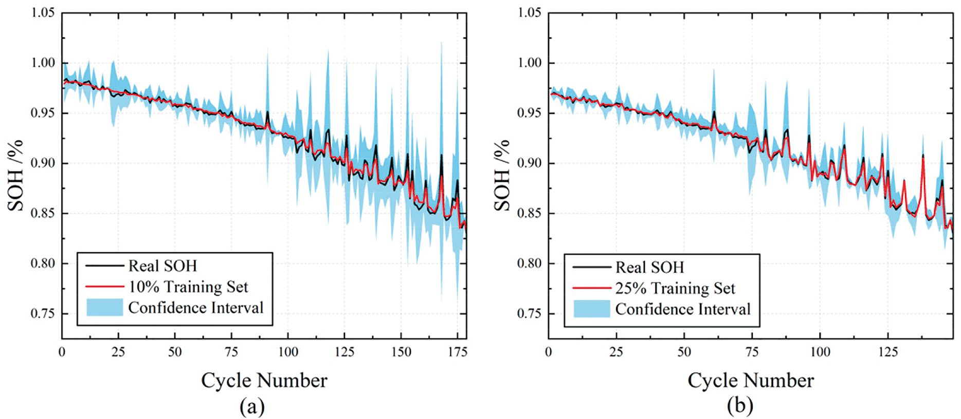
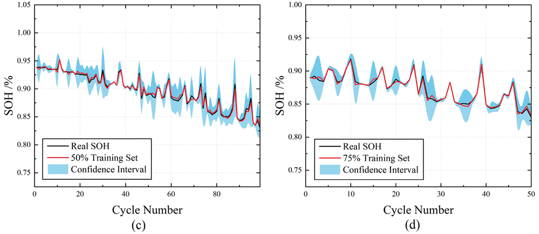
Figure 10: Results of SOH estimation by different proportions of training sets (a) Results using 10% training set (b) Results using 25% training set (c) Results using 50% training set (d) Results using 75% training set

Table 4 shows that when 75% of the data set is used as the training set, the model prediction accuracy is the highest, with MAE of 0.16% and RMSE of 0.22%. This finding not only validates the importance of sufficient data to improve the generalization ability of models, but also implies that models can learn and capture complex patterns and features more efficiently on larger datasets.

However, it is noted that the prediction performance of the state of charge does not increase linearly with the increase of the proportion of the training set. Specifically, the prediction results produced by the 25% training set are better than those of the 50% training set. The possible reasons behind this phenomenon are as follows. On one hand, the distribution characteristics of the data play a key role. A smaller proportion of the training set (such as 25%) may happen to cover more representative data samples, enabling the model to quickly capture key patterns, while the 50% training set may contain more noisy data or redundant information, interfering with the model’s learning of effective features and thus affecting the prediction accuracy. On the other hand, the sample diversities corresponding to different proportions of training sets are different. The data diversity under the 25% training set may, to some extent, just meet the learning needs of the model, and the model can make full use of these diverse and critical data for efficient learning; however, although the amount of data in the 50% training set increases, the newly added data may have a homogenization problem, unable to bring more effective information to the model, but increasing the computational burden and resulting in a decline in prediction performance. In addition, considering the data characteristics of lithium batteries themselves, the quality and correlation of data collected under different working conditions vary greatly. The proportion of high-quality and strongly correlated data in the 25% training set may be higher, enabling the model to focus on core features during the learning process and thus improve the prediction effect; while the 50% training set, due to the expansion of the data volume, introduces some low-quality and weakly correlated data, causing interference in the model’s learning process and affecting the final prediction performance.

In addition, the performance of the model with 25% training set ratio ranked second, which significantly demonstrated the good adaptability and learning ability of the BGNSM model under small sample conditions. It shows that the BGNSM lithium battery SOH estimation model can still maintain high efficiency in the case of relatively scarce data, and can effectively use limited information to learn and predict, which reflects the strong ability of this model to process small sample data. In contrast, the performance of the model under the 50% and 10% training set ratio is inferior to the first two, and the performance of the model gradually decreases with the reduction of the training data, but the decline is not linear.

It can be clearly observed from the visual display of Fig. 10 that when the proportion of training set is set to 25% and 50%, the predicted curve and the actual SOH curve show a high degree of fit, which is not only reflected in the close follow of the two trends, but also reflected in the narrow confidence interval of the predicted results. This finding further firmly proves the ability of the BGNSM model proposed in this paper to make accurate predictions in the case of small samples.

The data size plays a key role in the model training effect, so the training set size should be reasonably selected according to the specific task and data situation in practical application to balance the relationship between computing resources and model performance.

5.6 Model Performance under Different Working Conditions

In order to further verify the estimation accuracy of BGNSM model under complex working conditions and noisy environment, this study carefully constructed three typical simulation scenarios and systematically analyzed the performance of the model under non-ideal conditions:

1. Simulation of urban congestion conditions: Aiming at random current disturbance caused by frequent start and stop of urban roads, based on the original constant current test data, the current signal is superimposed with a normal distribution random noise (σ = 0.05) with a amplitude of 5%, so as to restore the unpredictable fluctuation characteristics of current in actual traffic.

2. Construction of rapid acceleration pulse conditions: In order to simulate the sudden current change in the process of rapid acceleration of the vehicle, a rule is set in the original charge and discharge sequence—insert 1 unit amplitude current pulse (ΔI = 1A) every 5 cycles, so as to test the response ability of the model to the dynamic sudden condition.

3. Design of white noise interference conditions: Considering sensor noise or external electromagnetic interference in practical applications, Gaussian white noise with standard deviation of 0.1 (SNR = 20 dB) is injected into the original data to build a typical noise interference scene.

The experimental results are shown in Fig. 11. In Fig. 11a, the predicted curve is highly consistent with the actual SOH curve, and the confidence interval completely covers the fluctuation range of the actual SOH, which fully reflects the strong robustness of the model to random disturbance. Fig. 11b shows that under the condition of rapid acceleration pulse, although the confidence interval is extended due to the sudden change of pulse, the prediction curve still accurately tracks the change trend of SOH, which verifies the adaptability of the model to the non-stationary condition. In Fig. 11c, the predicted curve is consistent with the actual SOH trend, and the confidence interval stably covers the actual value, confirming the reliable estimation ability of the model in a noisy environment. Through the system verification of the three types of working conditions, combined with the quantitative relationship between the prediction curve, actual value and confidence interval in the figure, the high-precision estimation ability of BGNSM model under complex working conditions and noise interference is fully demonstrated, providing strong experimental support for its engineering application.

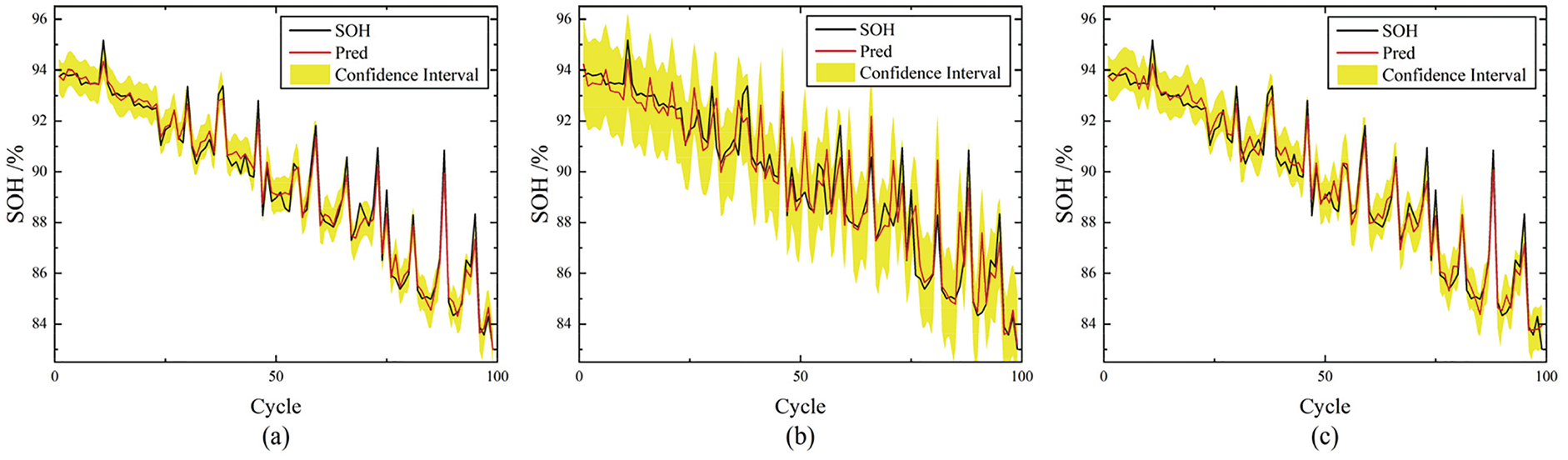
Figure 11: Results of SOH estimation under different working conditions (a) Results under urban congestion conditions (b) Results under rapid acceleration pulse conditions (c) Results under white noise interference conditions

Under three typical working conditions, the SOH estimation effect of BGNSM model, Variational Mode Decomposition (VMD) and Empirical Mode Decomposition (EMD) algorithm is further compared and analyzed.

As illustrated in Fig. 12: In subfigure (a), the BGNSM model demonstrates significantly superior tracking precision for real SOH values compared to both VMD and EMD methods. Notably, the latter two exhibit substantial fluctuations and pronounced deviations from true SOH. Subfigure (b) reveals that the BGNSM model maintains close alignment with the SOH trajectory, whereas VMD and EMD algorithms suffer from delayed and skewed predictions due to sensitivity to pulse-induced abrupt changes. Subfigure (c) further highlights BGNSM’s robustness, as its prediction curve achieves near-perfect consistency with actual SOH values. In stark contrast, VMD and EMD algorithms display severe instability under noise interference, manifesting erratic oscillations and significantly degraded estimation accuracy. This discrepancy arises from the intrinsic limitations of empirical mode decomposition methods (VMD and EMD), whose signal-dependent nature renders them vulnerable to mode aliasing when processing non-stationary signals such as pulsed waveforms. By contrast, the BGNSM framework circumvents these constraints through its integration of NIGP’s local kernel function, which adaptively captures nonlinear current-capacity relationships without relying on decomposition-based prior assumptions. In conclusion, comparative analysis under complex operational conditions and noisy environments confirms that the BGNSM model outperforms conventional decomposition-based approaches in three critical aspects: SOH estimation accuracy, dynamic trend tracking capability, and noise-resistant stability.

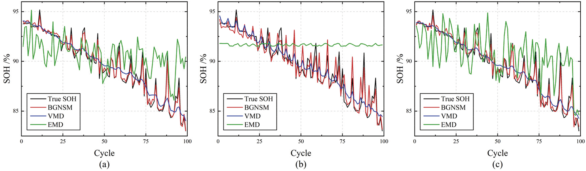
Figure 12: Results of SOH estimation under different working conditions by different models (a) Results under urban congestion conditions by different models (b) Results under rapid acceleration pulse conditions by different models (c) Results under white noise interference conditions by different models

6  Conclusion

In this study, we propose the BGNSM, a novel stack-based framework for predicting the SOH of LIBs. It combines the strengths of BWO-GPR and NIGP models, outperforming single models and conventional methods. By using NIGP’s noise-handling and BWO-GPR’s hyperparameter optimization, it captures battery degradation trends accurately. Also, it shows excellent predictive ability with small samples, laying a foundation for further exploration in such scenarios.

However, the BGNSM has limitations. Firstly, in larger datasets, the BGNSM can’t maintain small-sample efficiency. Its current architecture may not handle extensive data well, causing longer processing times. Second, although validated on lithium iron phosphate batteries, its generalization to ternary chemistry or extreme temperatures (e.g., −20°C to 45°C) is still untested. Finally, calibrating its hyperparameters demands expertise and is time-consuming, risking human errors that could undermine the model’s overall performance and reliability.

Despite significant success in predicting SOH of LIBs with high accuracy and narrow confidence intervals, future research should focus on optimizing model complexity and resources for better efficiency, integrating multi-source data like temperature and pressure to boost accuracy, extending scalability and adaptability for diverse batteries and systems, and developing online learning systems for real-time SOH monitoring.

Acknowledgement: Not applicable.

Funding Statement: This research was partly supported by the National Natural Science Foundation of China (Project No. 62273176), “Joint Laboratory Project of Intelligent Power and Control Applications” (Project No. 1003-KFA24090), and the National Key Research and Development Program of China (Project No. 2024YFB3311401).

Author Contributions: The authors confirm contribution to the paper as follows: Conceptualization, Pu Yang and Wanning Yan; methodology, Wanning Yan; software, Wanning Yan; validation, Pu Yang, Lei Chen and Lijie Guo; formal analysis, Wanning Yan; investigation, Wanning Yan; resources, Rong Li; data curation, Wanning Yan; writing—original draft preparation, Wanning Yan; writing—review and editing, Pu Yang, Wanning Yan, Rong Li, Lei Chen and Lijie Guo; visualization, Wanning Yan; supervision, Pu Yang, Rong Li, Lei Chen and Lijie Guo; project administration, Pu Yang; funding acquisition, Rong Li. All authors reviewed the results and approved the final version of the manuscript.

Availability of Data and Materials: The data that support the findings of this study are available from the Corresponding Author, Pu Yang, upon reasonable request.

Ethics Approval: Not applicable.

Conflicts of Interest: The authors declare no conflicts of interest to report regarding the present study.

References

1. Yang R, Xiong R, Ma S, Lin X. Characterization of external short circuit faults in electric vehicle Li-ion battery packs and prediction using artificial neural networks. Appl Energy. 2020;260(10):114253. doi:10.1016/j.apenergy.2019.114253. [Google Scholar] [CrossRef]

2. Cai L. A unified GPR model based on transfer learning for SOH prediction of lithium-ion batteries. J Process Control. 2024;144(2):103337. doi:10.1016/j.jprocont.2024.103337. [Google Scholar] [CrossRef]

3. Fan K, Wan Y, Jiang B. State-of-charge dependent equivalent circuit model identification for batteries using sparse Gaussian process regression. J Process Control. 2022;112(6):1–11. doi:10.1016/j.jprocont.2021.12.012. [Google Scholar] [CrossRef]

4. Sun D, Yu X, Wang C, Zhang C, Huang R, Zhou Q, et al. State of charge estimation for lithium-ion battery based on an Intelligent Adaptive Extended Kalman Filter with improved noise estimator. Energy. 2021;214:119025. doi:10.1016/j.energy.2020.119025. [Google Scholar] [CrossRef]

5. Song Y, Liu D, Liao H, Peng Y. A hybrid statistical data-driven method for on-line joint state estimation of lithium-ion batteries. Appl Energy. 2020;261:114408. doi:10.1016/j.apenergy.2019.114408. [Google Scholar] [CrossRef]

6. Ren D, Liu X, Feng X, Lu L, Ouyang M, Li J, et al. Model-based thermal runaway prediction of lithium-ion batteries from kinetics analysis of cell components. Appl Energy. 2018;228(57):633–44. doi:10.1016/j.apenergy.2018.06.126. [Google Scholar] [CrossRef]

7. Ke Y, Long M, Yang F, Peng W. A Bayesian deep learning pipeline for lithium-ion battery SOH estimation with uncertainty quantification. Qual Reliab Eng. 2024;40(1):406–27. doi:10.1002/qre.3424. [Google Scholar] [CrossRef]

8. Xiong R, Yu Q, Shen W, Lin C, Sun F. A sensor fault diagnosis method for a lithium-ion battery pack in electric vehicles. IEEE Trans Power Electron. 2019;34(10):9709–18. doi:10.1109/TPEL.2019.2893622. [Google Scholar] [CrossRef]

9. Liu P, Liu C, Wang Z, Wang Q, Han J, Zhou Y. A data-driven comprehensive battery SOH evaluation and prediction method based on improved CRITIC-GRA and att-BiGRU. Sustainability. 2023;15(20):15084. doi:10.3390/su152015084. [Google Scholar] [CrossRef]

10. Hu X, Jiang H, Feng F, Liu B. An enhanced multi-state estimation hierarchy for advanced lithium-ion battery management. Appl Energy. 2020;257:114019. doi:10.1016/j.apenergy.2019.114019. [Google Scholar] [CrossRef]

11. Che Y, Deng Z, Lin X, Hu L, Hu X. Predictive battery health management with transfer learning and online model correction. IEEE Trans Veh Technol. 2021;70(2):1269–77. doi:10.1109/TVT.2021.3055811. [Google Scholar] [CrossRef]

12. Wang S, Ren P, Takyi-Aninakwa P, Jin S, Fernandez C. A critical review of improved deep convolutional neural network for multi-timescale state prediction of lithium-ion batteries. Energies. 2022;15(14):5053. doi:10.3390/en15145053. [Google Scholar] [CrossRef]

13. Park K, Choi Y, Choi WJ, Ryu HY, Kim H. LSTM-based battery remaining useful life prediction with multi-channel charging profiles. IEEE Access. 2020;8:20786–98. doi:10.1109/ACCESS.2020.2968939. [Google Scholar] [CrossRef]

14. Wang F, Zhai Z, Zhao Z, Di Y, Chen X. Physics-informed neural network for lithium-ion battery degradation stable modeling and prognosis. Nat Commun. 2024;15(1):4332. doi:10.1038/s41467-024-48779-z. [Google Scholar] [PubMed] [CrossRef]

15. Lee JH, Lee IS. Estimation of online state of charge and state of health based on neural network model banks using lithium batteries. Sensors. 2022;22(15):5536. doi:10.3390/s22155536. [Google Scholar] [PubMed] [CrossRef]

16. Sabiri B, Asri ELB, Rhanoui M. Efficient deep neural network training techniques for overfitting avoidance. In: Enterprise information systems. Cham, Switzerland: Springer Nature Switzerland; 2023. p. 198–221. doi:10.1007/978-3-031-39386-0_10. [Google Scholar] [CrossRef]

17. Grecos C, Shirvaikar MV, Kehtarnavaz N. Heuristic approaches for porting deep neural networks onto mobile devices. In: Real-Time Image Processing and Deep Learning 2021; 2021 Apr 12–17; Online. p. 1173602. doi:10.1117/12.2580047. [Google Scholar] [CrossRef]

18. Zhao X, Wang W. Semi-supervised medical image segmentation based on deep consistent collaborative learning. J Imaging. 2024;10(5):118. doi:10.3390/jimaging10050118. [Google Scholar] [PubMed] [CrossRef]

19. Cui Z, Yang Z, Zhou Z, Mou L, Tang K, Cao Z, et al. Deep neural network explainability enhancement via causality-erasing SHAP method for SAR target recognition. IEEE Trans Geosci Remote Sens. 2024;62(11):5213415. doi:10.1109/TGRS.2024.3405942. [Google Scholar] [CrossRef]

20. Zhuge Y, Yang H, Wang H. Overview of machine learning-enabled battery state estimation methods. In: 2023 IEEE Applied Power Electronics Conference and Exposition (APEC); 2023 Mar 19–23; Orlando, FL, USA. p. 3028–35. doi:10.1109/APEC43580.2023.10131605. [Google Scholar] [CrossRef]

21. Wu Y, Wang T, Huang Y, Li Z, Xu L, Li DH, et al. A novel correlation-based approach for combined estimation of state of charge and state of health of lithium-ion batteries. J Energy Storage. 2024;96(4):112655. doi:10.1016/j.est.2024.112655. [Google Scholar] [CrossRef]

22. Ding C, Guo Q, Zhang L, Wang T. A hybrid data-driven approach for state of health estimation in lithium-ion batteries. Energy Sources Part A Recovery Util Environ Eff. 2024;46(1):67–83. doi:10.1080/15567036.2024.2399740. [Google Scholar] [CrossRef]

23. Bao C, Pu Y, Zhang Y. Fractional-order deep backpropagation neural network. Comput Intell Neurosci. 2018;2018:7361628. doi:10.1155/2018/7361628. [Google Scholar] [PubMed] [CrossRef]

24. Cheng R, Jin Y. A social learning particle swarm optimization algorithm for scalable optimization. Inf Sci. 2015;291(2):43–60. doi:10.1016/j.ins.2014.08.039. [Google Scholar] [CrossRef]

25. Zhang X, Lin Q. Three-learning strategy particle swarm algorithm for global optimization problems. Inf Sci. 2022;593(24):289–313. doi:10.1016/j.ins.2022.01.075. [Google Scholar] [CrossRef]

26. Wang C, Cui N, Cui Z, Yuan H, Zhang C. Fusion estimation of lithium-ion battery state of charge and state of health considering the effect of temperature. J Energy Storage. 2022;53(2):105075. doi:10.1016/j.est.2022.105075. [Google Scholar] [CrossRef]

27. Chen L, Bao X, Lopes AM, Xu C, Wu X, Kong H, et al. State of health estimation of lithium-ion batteries based on equivalent circuit model and data-driven method. J Energy Storage. 2023;73(4):109195. doi:10.1016/j.est.2023.109195. [Google Scholar] [CrossRef]

28. Samanta A, Williamson S. Machine learning-based remaining useful life prediction techniques for lithium-ion battery management systems: a comprehensive review. IEEJ J IA. 2023;12(4):563–74. doi:10.1541/ieejjia.22004793. [Google Scholar] [CrossRef]

29. Pan R, Liu T, Huang W, Wang Y, Yang D, Chen J. State of health estimation for lithium-ion batteries based on two-stage features extraction and gradient boosting decision tree. Energy. 2023;285(2):129460. doi:10.1016/j.energy.2023.129460. [Google Scholar] [CrossRef]

30. Chen Z, Zhang S, Shi N, Li F, Wang Y, Cui J. Online state-of-health estimation of lithium-ion battery based on relevance vector machine with dynamic integration. Appl Soft Comput. 2022;129(4):109615. doi:10.1016/j.asoc.2022.109615. [Google Scholar] [CrossRef]

31. Pathmanaban P, Arulraj P, Raju M, Hariharan C. Optimizing electric bike battery management: machine learning predictions of LiFePO4 temperature under varied conditions. J Energy Storage. 2024;99(2):113217. doi:10.1016/j.est.2024.113217. [Google Scholar] [CrossRef]

32. Wang J, Zhang C, Meng X, Zhang L, Li X, Zhang W. A novel feature engineering-based SOH estimation method for lithium-ion battery with downgraded laboratory data. Batteries. 2024;10(4):139. doi:10.3390/batteries10040139. [Google Scholar] [CrossRef]

33. Wang P, Zhang J, Cheng Z. State of health estimation of Li-Ion battery based on least squares support vector machine error compensation model. Power Syst Technol. 2022;46(2):613–23. doi:10.13335/j.1000-3673.pst.2021.0045. [Google Scholar] [CrossRef]

34. Jiang N, Zhang J, Jiang W, Ren Y, Lin J, Khoo E, et al. Driving behavior-guided battery health monitoring for electric vehicles using extreme learning machine. Appl Energy. 2024;364(27):123122. doi:10.1016/j.apenergy.2024.123122. [Google Scholar] [CrossRef]

35. Wang J, Deng Z, Yu T, Yoshida A, Xu L, Guan G, et al. State of health estimation based on modified Gaussian process regression for lithium-ion batteries. J Energy Storage. 2022;51:104512. doi:10.1016/j.est.2022.104512. [Google Scholar] [CrossRef]

36. Li H, Peng R, Zhu Z, Zhu R. An intelligent state of health estimation method for lithiumion batteries. In: New materials, machinery and vehicle engineering. Amsterdam, NY, USA: IOS Press; 2023. p. 313–9. doi:10.3233/atde230153. [Google Scholar] [CrossRef]

37. Liu Q, Bao X, Guo D, Li L. Bayesian optimization algorithm-based Gaussian process regression for in situ state of health prediction of minorly deformed lithium-ion battery. Energy Sci Eng. 2024;12(4):1472–85. doi:10.1002/ese3.1678. [Google Scholar] [CrossRef]

38. Guo W, Sun Z, Vilsen SB, Meng J, Stroe DI. Review of grey box lifetime modeling for lithium-ion battery: combining physics and data-driven methods. J Energy Storage. 2022;56:105992. doi:10.1016/j.est.2022.105992. [Google Scholar] [CrossRef]

39. von Bülow F, Meisen T. A review on methods for state of health forecasting of lithium-ion batteries applicable in real-world operational conditions. J Energy Storage. 2023;57:105978. doi:10.1016/j.est.2022.105978. [Google Scholar] [CrossRef]

40. Deng Z, Hu X, Lin X, Che Y, Xu L, Guo W. Data-driven state of charge estimation for lithium-ion battery packs based on Gaussian process regression. Energy. 2020;205(5):118000. doi:10.1016/j.energy.2020.118000. [Google Scholar] [CrossRef]

41. Benesty J, Chen J, Huang Y. On the importance of the Pearson correlation coefficient in noise reduction. IEEE Trans Audio Speech Lang Process. 2008;16(4):757–65. doi:10.1109/TASL.2008.919072. [Google Scholar] [CrossRef]

42. Xue Y, Liu Y, Ji C, Xue G, Huang S. System identification of ship dynamic model based on Gaussian process regression with input noise. Ocean Eng. 2020;216(3):107862. doi:10.1016/j.oceaneng.2020.107862. [Google Scholar] [CrossRef]

43. Zhong C, Li G, Meng Z. Beluga whale optimization: a novel nature-inspired metaheuristic algorithm. Knowl Based Syst. 2022;251(1):109215. doi:10.1016/j.knosys.2022.109215. [Google Scholar] [CrossRef]