Leveraging the WFD2020 Dataset for Multi-Class Detection of Wheat Fungal Diseases with YOLOv8 and Faster R-CNN

1  Introduction

After rice and maize, wheat is the third most consumed grain in the world. It is an essential source of protein and calories for all diets [1]. However, fungal infections reduce both yield and quality, posing a serious threat to wheat production, resulting in large financial losses. These diseases can damage both the visible and invisible portions of wheat plants, such as leaves, stems, and spikes, as well as invisible root components, which are caused by pathogenic fungi and manifest as a variety of symptoms [2]. The most common fungal infections worldwide are rust diseases such as leaf rust, yellow rust, and powdery mildew, which pose a hazard to the wheat supply chain [3]. These diseases develop in areas with favorable climates, such as Punjab, India, and in extreme cases, yellow rust alone has been known to reduce wheat production by 20%−30%. Fungal diseases have economic consequences that go beyond yield loss. Food security and farmer income are affected by lowering market prices and grain quality. In the near future, there will likely be nine billion people on the planet; therefore, the demand for wheat will be approximately 60% [4] which will increase the demand for wheat and highlight the need for sustainable wheat crop management techniques. Effective treatment of wheat fungal infections is especially important in developing countries, because yields per hectare are generally lower than those in developed countries.

The early detection of fungal infections is necessary to minimize these losses. Farmers may carry out focused treatments with accurate identification by optimized use of excessive fungicide sprays, thereby saving money and the environment. However, identification of fungal diseases poses various challenges. Images of wheat extracts sometimes have complex backgrounds, such as hands, soil, or foliage, which may minimize disease identification. Furthermore, the growing phases of crop-related diseases make the classification more difficult. Recent advances in artificial intelligence (AI), particularly deep learning, have provided promising solutions for automated plant disease identification. There are various models of R-CNN which are most rapidly used model for multi-class object detection and have also proven the advantageous in identifying several diseases in a single image such as R-CNN, Faster R-CNN [5,6]. These models offer significant gains over conventional image classification techniques that use Convolutional Neural Networks (CNNs) to locate diseased areas [7–9]. The selection of the best architecture for domain-specific applications remains a challenging task.

This study used multiclass object detection models to provide an automated system for identifying and locating fungal diseases in wheat fields. First, Tensorflow-based, Faster R-CNN, and SSD models with different variants of ResNet backbones were utilized. The study then examined the YOLOv8 model, which was built on PyTorch and showed excellent performance in identifying both single and multiple disease classifications. In addition to highlighting the comparative analysis of various models, this study offers a novel method for precise fungal disease localization and categorization. The remainder of this paper is organized as follows. An analysis of research on deep-learning-based object detection models for the diagnosis of plant diseases is presented in Section 2. The experimental setup and dataset preparation are described in detail in Section 3. The architecture and experimental performance of the Faster R-CNN and YOLOv8 models are presented in Section 4. Finally, Section 5 concludes the study and provides suggestions for further investigation.

2  Related Work

To classify and divide plant diseases, scientists have used well-known machine learning classifiers such as Support Vector Machines (SVM) and k-means clustering. However, as deep learning has grown, numerous researchers have become more interested in multiclass object recognition methods than in identifying plant diseases. Over the past few decades, deep learning algorithms have made significant progress in solving computer vision-related problems. This was primarily because a large number of datasets were available. GPUs, or graphics processing units, are examples of high-computational power devices that are required for processing large amounts of data. Using deep learning-based models, numerous researchers have shown amazing results in the detection of plant diseases [10–14]. As such, the literature has been divided into two main sections, these two methods for identifying wheat crop diseases are: (a) using machine learning algorithms to classify the diseases, and (b) using deep learning algorithms to detect the diseases. The following is a thorough analysis of studies on wheat crop disease detection.

2.1 Work Done on the Classification of Wheat Diseases Using Machine-Learning Approaches

Bravo et al. classified several types of rust infestation in wheat crops. The authors gathered a primary dataset of images of diseased wheat leaves from two classes, yellow rust and healthy wheat in their investigation. They reported an accuracy of 96.00% using the Quadratic Discrimination method [15]. Subsequently, Moshou et al. [16] used primary images of wheat leaf diseases, including both diseased and healthy leaves. Using the multilayer perceptron technique, they attained a 99.00% accuracy rate in their intelligent disease identification system. Similarly, the SVM classifier was used by Siricharoen et al. [17] to analyze raw datasets of diseased wheat leaves, which were further divided into three classes: septoria, yellow rust, and healthy wheat. For the datasets in controlled and uncontrolled environments, they obtained accuracy rates of 95% and 79%, respectively. Shafi et al. [18] used a primary collection of images of wheat diseases that contained three classes: susceptible, resistant, and healthy wheat. They first collected 2000 images, which were then further processed to eliminate intricate backdrops and adjusted for various lighting conditions. They used a dataset of 1640 images of wheat crop diseases. They applied CatBoost, employing the Gray-Level Co-occurrence Matrix as a feature extraction method that could discriminate between different types of rust infections with an accuracy of 92.30%. In [19], authors used deep convolutional neural network using hyper-spectral images of three diseased classes. An accuracy rate of 85.00% had been reported to classify the wheat leave diseases. In [20], the authors used VGG16 transfer learning model for distinguishing wheat diseases with 1400 images with the recognition accuracy of 98.00%. In [21], the authors used the elliptical-maximum metric learning to define the severity level to identify the wheat leaf diseases and reported the accuracy of 94.16%. The authors in [22] implemented the YOLOv8 model using 2569 images and they achieved 0.72 mAP for detecting various plant disease species.

2.2 Work Done on the Classification and Detection of Wheat Diseases Using Deep Learning-Based Approaches

To estimate wheat crop production, Hasan et al. devised a method to recognize wheat spikes. The main problem that they identified was the separation of diseases from field image data in the presence of complicated backdrops, severe spike occlusions, and different illumination constraints. They used an annotation tool to mark wheat spikes manually after gathering a range of images from the fields. They used a region-based convolutional neural network (R-CNN) to identify and count wheat spikes. Consequently, they were able to identify wheat spikes in the test images with up to 94% accuracy. Picon et al. concentrated on the primary datasets of several wheat crop diseases. They classified different diseases of wheat crops using a convolutional neural network-based architecture, namely the ResNet150 model, and reported an accuracy of 96.00%. After that, Schirrmann et al. [25] distinguished between several wheat crop diseases using the ResNet18 model. They achieved an accuracy rate of 95.00% when separating wheat plants free of stripe rust infection from healthy plants. However, instead of concentrating on classification, researchers have turned their attention to detection, trying to find the precise location of diseases in image data. To precisely locate the disease, they used a variety of object detection-based methods, including the Faster R-CNN and R-CNN. In addition, Li et al. used the Faster R-CNN and RetinaNet feature extractor with a global heat dataset, which included images of wheat ears at various phases (such as the filling and maturity stages). Using RetinaNet and Faster R-CNN, they achieved 82.00% and 72.00% accuracy, respectively [26]. Similarly, Liu et al. detected stripe rust infections captured in both oriental and horizontal ways using an object detection-based algorithm. The average precision for identifying wheat stripe rust is 0.61. The work done on categorizing and identifying wheat crop diseases using machine- and deep-learning-based methods is summarized in Table 1.

3  Dataset Description

Currently, very few publicly available datasets of wheat disease images affect various disease patterns in wheat crops. Those images depict the diverse patterns that have been collected using fixed cameras or smartphones under field conditions. These images include additional information, such as weeds, soil, and human hands touching the damaged leaves, and some diseased images also contain healthy plants. The WFD2020 dataset focuses on fungal infections affecting wheat crop and has been utilized in the present study. This dataset is accessible to the general public for research purposes at “http://wfd.sysbio.ru/” (accessed on 13 March 2025) [27]. It comprises ten classes of fungal diseases that affect wheat crops. However, for experimentation purposes, three disease classes (yellow rust, leaf rust, and powdery mildew) were used. Examples of images showing fungal infections in wheat are given in Fig. 1; each image shows a single diseased class. These two diseases are depicted in two distinct images are shown in Fig. 2. In real-world situations, identification of various diseases is difficult. Therefore, there is a need to develop an automated system that uses images to detect diseases and their locations. However, the development of such systems requires thorough knowledge of hardware resources, technical support, and annotation tools.

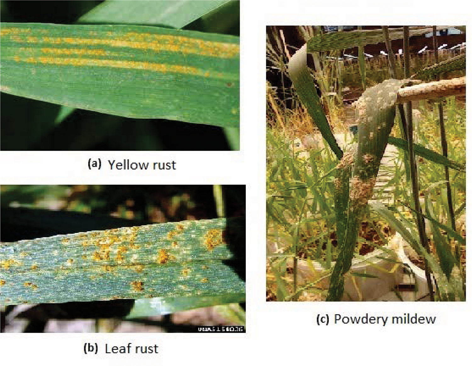
Figure 1: Sample of images containing single disease

Figure 2: Image sample containing multi-diseases (i.e., leaf rust and powdery mildew)

3.1 Dataset Annotation

For object recognition, each object in an image must have a ground truth label assigned to it. This label contains the precise details of the shape and placement of the object inside the image [28]. Experts have thoroughly verified bounding-box annotations to ensure the accuracy of disease identification. Automated testing helps detect and rectify errors in datasets. Errors can have an impact on the model performance, leading to erroneous detections or inadequate object localization. Accurately assigning class labels to different objects can characterize and identify objects, which is the primary goal of image annotation. Many tools are currently available for annotating images, including LabelImg, Labelme, VGG annotator, and AI-based Computer vision annotation tools (CVAT). Among them, the Python-developed LabelImg and AI-based CVAT tools are the most widely used tools to annotate images. Moreover, using these tools, we can annotate our images into different formats: YOLO, PASCAL VOC, and CreateML, depending on the type of object-detection model used. However, in this study, we used two different annotation formats: the PASCAL VOC format that is,∗.xml for executing the Tensorflow-based models, the annotations using LabelImg, and the other is for the YOLOv8 object detection model which requires YOLO (∗.txt) formats for object detection using AI-based CVAT tool. The most frequently used format is ∗.xml and ∗.txt, where the object class was identified using bounding-box coordinate data. Bounding boxes use the x- and y-coordinates to determine the location of the target object inside an image, with width, height, and depth parameters to specify the dimensions of the object. Note that the image and its generated annotation file have the same name. For instance, ten annotation files corresponding to the ten sampled images were generated. These images and their annotations were then combined and sent to the model for further processing and training. Table 2 shows the sample information, where there are 350 high-resolution images, which are divided into four classes: multi-diseases (50 images), leaf rust (100 images), powdery mildew (100 images), and yellow rust (100 images). To assure accuracy, professionals carefully annotated images taken from various farm environments, capturing the unique visual characteristics of each disease. A deliberate emphasis was placed on the lower frequency of multi-disease cases to test the model performance in underrepresented diseases. Pre-processing techniques, such as normalization and scaling, guarantee data quality while maintaining important characteristics. During the training and testing of the models, single and co-occurring plant diseases were considered in real-life situations.

3.1.1 Annotation Description for Tensorflow-Based Models

To annotate the images, we used the LabelImg tool, which generally uses the ∗.xml formats. The images and annotations utilized to train the model are listed in Table 2. A total of 350 images were used, and 753 annotated objects were generated and divided into three classes: powdery mildew, leaf rust, and yellow rust. Thirty-four images were used during the testing process. Out of these 34 images, 24 contained only information about one disease-, and 10 had multiple diseases. For the three diseased groups, 99 ground-truth annotations were generated from the test images. For example, 46, 16, and 37 annotated objects were generated for leaf rust, yellow rust, and powdery mildew, respectively. The annotations of the sampled diseased images are given along with their associated annotated files, as shown in Figs. 3 and 4, respectively.

Figure 3: An illustration of annotation of multiple objects with in an image

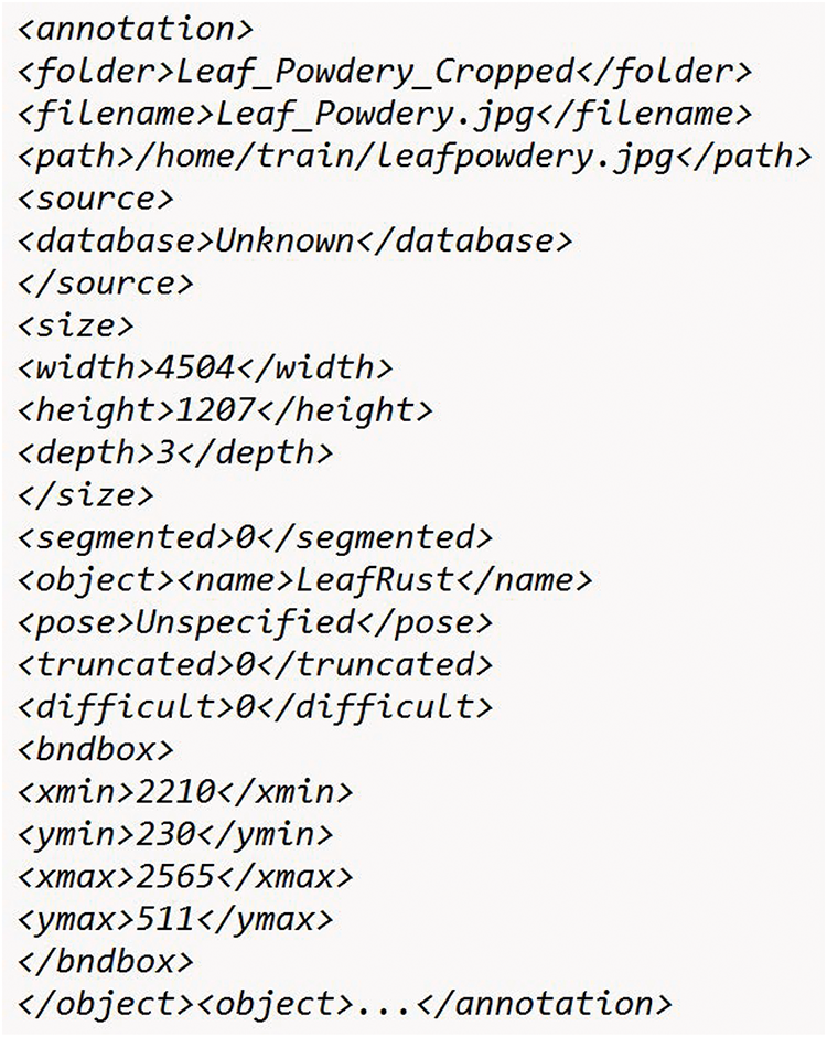
Figure 4: Annotated file’s attributes

3.1.2 Annotation Description for Pytorch-Based Models

Further, to experiment with the YOLO model, we used the AI-based CVAT tool to annotate the same dataset as mentioned above. It is an open-source image annotation tool written in JavaScript and Python. Using this tool, we can annotate images in different formats according to the requirements of the object detection models. A total of 350 images were used and 619 annotated objects related to the three given classes were generated. Out of these 619 annotated objects, 192, 257, and 170 instances were generated through distinct classes: yellow rust, powdery mildew, and leaf rust diseases, respectively.

4  Methodology

In this study, we used two deep learning model frameworks, one is TensorFlow and other one PyTorch-based. Initially, we considered the two TensorFlow-based object detection models, i.e., Faster R-CNN and SSD with different backbones and image sizes. Subsequently, we used the PyTorch-based YOLOv8 state-of-the-art algorithm. Now, let us understand the basics of object-detection algorithms. Object detection is one of the most popular computer vision methods for identifying objects in an image. Accurately locating an object within an image frequently entails producing a higher number of region proposals from the input images. The main objective of detection techniques is to determine and project an object’s location. An object can be identified using four characteristics: enclosure, color, texture, and scale. More specifically, a bounding box with a confidence score is usually the result of an object-detection model. The confidence score, which lies between 0 and 1, indicates how confident the model is in order to correctly identify the object present inside the bounding box. The detection process consists of two main tasks: the classification and location of the target area. Here, localization focuses on accurately drawing the bounding box around an object, and image identification identifies the presence of an object in an image. These bounding boxes are typically determined by the x- and y-axis coordinate values. Broadly, we can classify various object detection models into two categories, an overview of which is given in the following section.

a) Region proposal-based object detection models Region proposal-based object detection models are commonly used to improve high-level features and predict bounding box coordinates. These models are also known as two-stage detectors; in the first stage, they create the region of interest, and in the next stage, they perform the classification task. The performance of these detector models depends on high-speed hardware components such as GPUs and TPU-powdered machines. Additionally, the selection of object detection models, such as R-CNN, Fast R-CNN, Faster R-CNN, etc., has a direct impact on the performance of the model.

b) Regression and classification-based One-stage detectors directly map the bounding box coordinates and input image pixels to forecast class probabilities. You Only Look Once (YOLO) and single-shot multibox detectors (SSDs) are the two most popular one-stage detectors. This study explored variants of SSDs, Faster R-CNN, and YOLOv8 models to detect various fungal infections in wheat.

Here is a brief discussion about these models:

(i) Single-shot detectors (SSDs): An SSD model detects objects in an image in a single shot. Using anchor boxes of various sizes and aspect ratios, this single-stage detector predicts object instances that constitute the classifier and regressor of the complete network. Each convolutional layer generates feature maps that are then combined using a post-processing technique called greedy nonmax suppression, producing a range of bounding boxes for class discrimination. These boxes were then employed to suppress duplicate detections. The most prominent application of the SSD technique is to detect large-scale objects and deliver highly accurate results with faster processing times than the faster R-CNN model. One-stage detectors typically operate faster than two-stage detectors.

(ii) Faster R-CNN: The Faster R-CNN model, proposed by Ren et al. in 2015 [29], operates in two steps. The first stage involves generating region proposals, while the second stage performs classification. In this network architecture, region proposals are generated efficiently by RPNs (Region Proposal Networks) that work together with the detection network to share full-image convolutional characteristics. These RPNs can generate anchor boxes of various shapes, including square, long, wide, or large rectangular shapes. In addition, three different sizes may be available for these anchor boxes: small, medium, and large. The object recognition models in the current investigation were trained using pretrained TensorFlow object recognition models. Specifically, SSDs and faster R-CNNs are the two most widely used object recognition models [29,30]. A variety of pretrained object identification models are experimented with Table 3, which use different backbone CNN-based models that were selected based on their speed and mean average precision after training the model on the COCO dataset.

(iii) YOLOv8: The primary goal of current research is to detect objects in real-time with high accuracy, which makes it appropriate for applications that demand efficiency and speed, including autonomous systems and precision agriculture. The YOLOv8 model is the state-of-the-art algorithm used in various areas of agriculture such as disease detection, weed detection, etc. [31–34]. Even in devices with low processing power, deployment is guaranteed by their lightweight architecture, which includes innovations, such as enhanced feature pyramids and adaptive anchor computations. However, Faster R-CNN region proposal networks (RPNs), which focus on high accuracy and detailed object recognition, perform exceptionally well in tasks that require precise localization and classification in challenging situations, such as aerial analysis or medical imaging. When combined, these models meet a variety of needs; Faster R-CNN prioritizes accuracy and managing difficult settings, whereas YOLOv8 prioritizes speed and deployment flexibility [35].

4.1 Wheat Disease Detection Using Faster R-CNN

To identify the various fungal diseases that impact wheat crops, it is necessary to set up a workspace, specify the model, prepare the dataset, and set up a model architecture based on deep learning models. These model parameters must be trained and adjusted to increase the efficiency of the model in detecting wheat crop diseases. Table 4 lists the specifications of the hardware and software used to train the multi-objective detection models. The GPU-equipped device used in this work is a GeForce RTX 2080 Ti with 62.5 GB RAM, which is used to train the object detection models. Processing and training deep learning models within a few minutes is the main benefit of employing GPU-enabled machines. However, instead of wasting time on low-level GPUs, academics can concentrate on creating software applications and building neural networks for training and utilizing high-level GPUs. In addition, installing appropriate CUDA and cuDNN libraries necessitates an experimental procedure. The software can interact with particular GPU-enabled devices through the CUDA API, whereas cuDNN is a common deep-learning library used to train object identification models. In this study, version 8.5 of the cuDNN library and version 11.0 of the CUDA library were used for the current GPU requirements.

4.1.1 Model Architecture

Every object detection model (i.e., VGG16, ResNet50, ResNet101, etc.) aggregate features and function as fundamental models. Several researchers have used the ResNet50 model as a feature extractor for object detection [36]. Consequently, we used variant ResNet models as the basis for our investigation. The resulting model referred to as WFDetectorNet, outperforms in identifying several fungal diseases infecting the wheat crops. It is a Faster R-CNN model with a ResNet50 backbone built after fine-tuning various hyperparameters. Fig. 5 shows the architectural structure of the Faster R-CNN model, which is intended to recognize various fungal diseases in wheat crops. The images, annotations, and designated label class files are merged into a single binary file at the beginning of the detection procedure. This model then uses the ResNet50 model’s convolutional layers to produce a variety of region predictions. Region Proposal Networks (RPNs) are small neural networks that used for predictions. These proposals were generated using RPNs of various sizes and aspect ratios. To allow a range of aspect ratios and scale values, anchor boxes were generated with numerous sizes. An input image is projected using a predefined collection of bounding boxes with different scales and aspect ratios, known as anchor boxes. These anchor boxes are then used by the object detection algorithm to forecast the location and size of objects inside the image. Selecting a set of base anchor boxes with various aspect ratios and sizes is the first stage in generating anchor boxes at various scales. Anchor boxes are usually described by two parameters, width and height, which determine the dimensions of the anchor box, and a pair of (x, y) coordinates indicates the center of the anchor boxes. It is possible to specify predefined sizes and aspect ratios for the base anchor boxes. Consider two base anchor boxes, one of which is 128 × 64 in size and has an aspect ratio of 0.5, and the other is 64 × 128 in size and has an aspect ratio of 2.0. These foundation anchor boxes can be built at different scales, using them as templates. Scaling factors were used to scale the base anchor boxes and construct anchor boxes at various scales. Four scaling factors were used to train the model: 0.50, 0.25, 2.0, and 1.0, respectively. The following procedure was used to generate anchor boxes that were subsequently placed at different points throughout the image. The initial base anchor box comprises 128 × 64 pixels, with an aspect ratio of 0.5. The scaling values were adjusted to obtain anchor boxes of varying sizes: (32, 16), (128, 64), (64, 32), and (256, 128). Each scaled anchor box is positioned differently throughout the image. For example, in a 16 × 16 grid, we arranged them in the middle of each grid cell to create 256 anchor boxes for the base anchor box. The second base anchor box measured 64 × 128 pixels and had an aspect ratio of 2.0. -For the second base anchor box, which has an aspect ratio of 2.0 and dimension of 64 × 128. The scaled anchor boxes must be placed at various points throughout the image. For example, in a 16 × 16 grid arrangement, 256 anchor boxes were generated at the center of each grid cell to create the base anchor box. This yielded 512 anchor boxes with the appropriate aspect ratios. The actual sizes of the generated anchor boxes vary depending on the scaling factors, even if the base anchor box size is set to 256 × 256. These generated bounding boxes are sent to the Region of Interests (ROIs) in the pooling layer. This layer selects the most important features, which is similar to the CNN max-pooling layer. In addition, it converts feature maps of non-uniform sizes into fixed-size feature maps. Subsequently, the fully connected layers received these feature maps and the model began training. In addition, the training speed and test duration of the model were accelerated using the ROIs pooling layer. Moreover, the bounding boxes and class labels (softmax activation function) were predicted by the classifier and regressor simultaneously. The computational cost increases; therefore, the model produces numerous bounding boxes or region proposals. The bounding boxes were also eliminated by the non-maximum suppression (NMS) layer, which predicted the highest prediction confidence score.

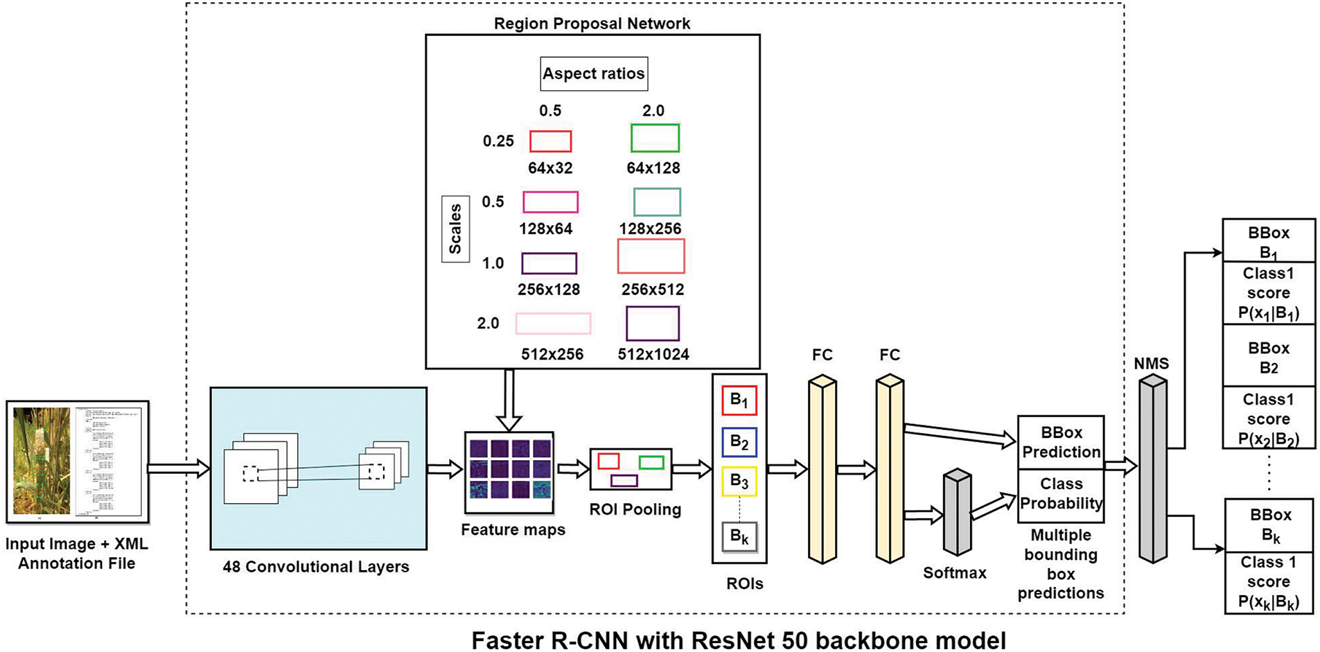
Figure 5: Model architecture Faster R-CNN for detector fungal disease of wheat crops

4.1.2 Training the Model

As previously mentioned in Table 3, the model for diagnosing fungal infections in wheat crops is trained using object detection models, particularly Faster R-CNN and SSDs. The TensorFlow object detection API was used to create a TFRecords file, which prepared the dataset for training. One benefit of binary-format files is that they use less disc space. The following procedures are involved in creating the TFRecords file. (a) All image files were annotated, thus generating an individual XML file for each image file. (b) Converting every ∗XML file to a ∗s.CSV file. (c) A label map file is created in which a distinct ID is allocated to each object class. Subsequently, these three files–images, annotations, and label maps–were combined to create a TFRecords file. During the generation of this binary file, the object detection model was customized using a model configuration file. A detailed description of the configuration files and default values for the object-detection model training is provided below.

•   Num_classes: The total number of objects that can be identified is referred to as the number of classes. The default value of this parameter on the COCO dataset is 80 classes, which can be changed depending on the number of objects in a given problem.

•   feature extractor: A feature extractor is similar to a CNN model that can extract relevant characteristics from annotated objects. VGG16, ResNet, InceptionNet, and other backbone models are the most frequently used models for object detection.

•   Scales: The configuration file’s scale parameter changes based on the object’s size. The default scale values are 0.25, 0.5, 1.0, and 2.0, which use a base anchor box to create four anchor boxes of varying sizes. The following formula shows how to retrieve the output anchor boxes: Output anchor boxes = [scale∗

•   Aspect_ratios: The aspect ratio is the width-to-height ratio between the anchor boxes. The default values of the aspect ratio were 0.5, 1.0, and 2.0, indicating optimal aspect ratio values. For example, for facial recognition its value will be 1.0; choosing 0.5 or 2.0 would be unreal because no face-in-face detection problem has a width that is half of its height or twice its width. Selecting the correct aspect ratio is a very important parameter in object detection. Therefore, selecting the appropriate value of the aspect ratio significantly reduce the amount of time required to train the model. The format of the output anchor boxes is as follows. Output anchor box = (width × (aspect ratio) ∗ height)

•   Height/width stride: Anchor boxes are created using height and width strides, always staying true to their nominal values, which are placed in the middle of the bounding boxes.

•   Batch_size: The number of samples in the neural network used for training in an epoch was determined by the batch size. Both image dimensions and hardware have significant effects on this value. Also, larger larger batch sizes require powerful GPU computer systems.

•   Num_steps: The total number of epochs multiplied by the ratio of the size of the training dataset to the batch size was used to obtain the number of steps.

•   Data_augmentation_options: Deep learning models require large amounts of data, which are necessary for a dataset that can be increased using augmentation techniques. Augmentation in object detection models can be performed better by adjusting the saturation, hue, and contrast properties.

•   Learning_rate: The learning rate modifies the network weights by adjusting the step size during training, thereby accelerating and stabilizing the network. A lower learning rate frequently results in better model performance, even if it slows down the learning process. During testing, the default value of the learning rate changed from 0.01 to 0.02.

At this point, the default parameters were used in a small number of experiments. Table 5 contains a description of the predefined parameters that were experimented with to determine baseline models.

4.1.3 Performance Evaluation Metrics

In deep learning, mean Average Precision (mAP) metrics are widely used to evaluate the efficiency of the detector algorithms. Typically, the performance of a detector model is assessed using only one metric. Adding average precision values? The average precision is the area under the precision-recall curve, and the mean accuracy percentage (mAP) may be calculated. The Intersection over Union (IoU) threshold value quantifies the degree of overlap between two bounding boxes, and is used to compute the average precision. IoU values can also show how similar the two bounding boxes are to each other. The IoU values lie between 0 and 1, where 1 denotes a perfect match between the predicted and ground-truth bounding boxes and 0 denotes no overlap. A comparison between the ground-truth values and predicted bounding boxes is presented in Fig. 6, which shows the execution of the intersection over the union operation. A bounding box can be used to annotate different objects that appear in an image to determine the ground truth value. For the majority of the evaluation tasks, the IoU is set to a threshold value of 0.5, which is considered the appropriate value. The IoU number can be used to assess the output. For example, mAP @ 0.5 is taken into account if the value of IoU is 0.5. In addition, True Positive (TP), False Positive (FP), and False Negative (FN) terminologies were used to represent recall and precision.

(i)   TP: When IoU ≥ 0.5, the ground-truth object is discovered with the appropriate class label.

(ii)   FP: When IoU is less than 0.5, the ground-truth item is recognized with the inaccurate class.

(iii)   FN: No evidence of the object’s ground truth.

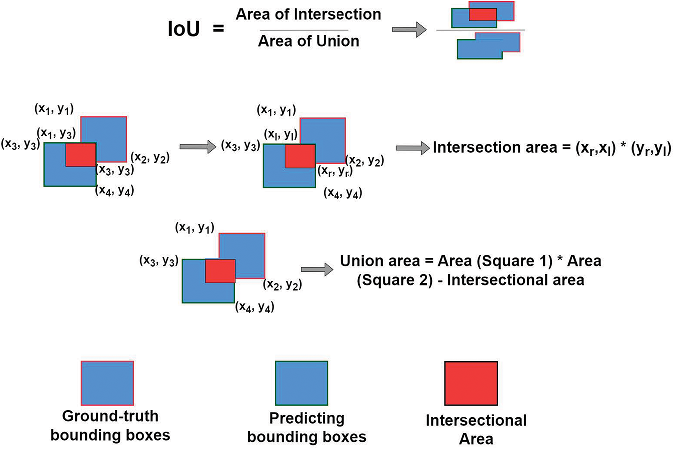
Figure 6: An illustration of Intersection over Union (IoU)

The precision of the object detection model is the percentage at which the appropriate objects in the image are accurately detected. It can also be applied to ascertain the quantity of genuinely favorable results, which can be stated as follows:

Precision=TPTP+FP≅TPTotalpredictions(1)

On the other hand, recall, which is expressed as follows, shows the success rate at which the model was able to recognize real positive cases, represented as:

Recall=TPTP+FN=≅TPTotalground−truths(2)

This is simply the area under the precision-recall curve. Over time, the meaning of “AP” has changed. The final metric is the mean average precision of the test data, which can be obtained by averaging the precision for each class. Each class is denoted by k and its mAP is computed across various IoU thresholds, as given below:

mAP=1n∑k=1k=nAPk(3)

Tables 6 and 7 present the average precision results obtained from various object detection models, including SSD (a one-stage detector) and Faster R-CNN (a two-stage detector), for identifying powdery mildew, yellow rust, and leaf rust diseases on wheat crops. A comparison of the mAP results for detecting several fungal infections of the wheat crop using SSD models is shown in Table 6. For 640 × 640 and 1024 × 1024 image sizes, we analyze SSD model changes using backbone models (ResNet50, ResNet101, and ResNet152). The SSD model with ResNet50 backbone, which was trained on 640 × 640 images, showed the lowest mAP of 0.23 among all of these models. Conversely, the mAP findings of the Faster R-CNN model with distinct backbone models (ResNet50, ResNet101, and ResNet152) across many image sizes (640 × 640, 1024 × 1024, and 800 × 1333) are presented in Table 7. The model having the highest mAP of 0.62 was obtained using the Faster R-CNN model, which was trained on images with a size of 800 × 1333 using the ResNet50 backbone. These evaluations show that the model produces reasonable results when identifying items with different sizes. Thus, the Faster R-CNN model with 800 × 1333 image size and ResNet50 backbone emerges as a fundamental model with promising results for wheat fungal disease detection. These findings are based on evaluation results from some object detector models-, and provide possible directions for additional development to improve overall performance.

4.1.4 Fine-Tuning the Model

The base model, Faster R-CNN with ResNet50 backbone, was fine-tuned after it was first trained on an 800 × 1333 image size. Several hyperparameters, including the batch size, learning rate, scale, aspect ratios, and total number of steps, have adjusted during the training process. In Table 8, a summary of the tests with various fine-tuning settings is presented. The basic model in Experiment 1 was trained using fixed values for the following parameters: aspect ratio = [0.5, 1.0, 2.0], scale = [0.25, 0.5, 1.0, 2.0], learning rate = 0.1, batch size = 2, and total number of steps = 25,000. The mAP value for this model is 0.62. In Experiment 2, the scale values were changed from [0.25, 0.5, 1.0, 2.0] to [0.625, 0.125, and 0.25] while maintaining the same values for the other variables. The results revealed no discernible differences even with this adjustment, which was made to detect diseased items of different sizes. The model is then trained with scales = [0.025, 0.5, 1.0] in Experiment 3, keeping the values for the other parameters constant. However, the mAP results do not show any appreciable variations. Consequently, we reset the scale values to their starting points, which are [0.25, 0.5, 1.0, 2.0], and we carried out further research to ascertain the proper aspect ratio values. In Experiment 4, a significant increase in mAP from 0.60 to 0.65 was noted when changing the aspect ratios from [0.5, 1.0, 2.0] to [0.5, 2.0]. Subsequently, we adjusted the learning rate and performed several tests. The learning rate was changed for experiments 5, 6, and 7 from 0.1, 0.001, 0.001, 0.003, and 0.003 to 0.0001, respectively, to determine the best learning rate. The mAP results decreased significantly. In Experiment 8, we reset the learning rate to 0.1 and increased the total number of steps from 25,000 to 40,000. With an mAP of 0.67, the model demonstrated a discernible increase in learning rate. Furthermore, the total number of steps was increased to 50,000 and 60,000 in Experiments 9 and 10, respectively. However, throughout these studies, the mAP levels varied which ranged from a relatively low value of 0.47 for experiment 9 to a comparatively high mAP of 0.67 for experiment 10. We then experimented with 11 with incremental steps = 60000, aspect ratio = [0.5, 2.0], learning rate = 0.1, and updated scales = [0.625, 0.125, 0.25, 0.5, 0.75, 1.0, 1.5, 2.0] to improve the prediction of proper bounding boxes corresponding to each ground-truth bounding box. Eventually, the mAP value was reduced from 0.67 to 0.60 while updating the scaling value. This implies that [0.25, 0.5, 1.0, 2.0] is the ideal scale values for predicting wheat crop diseases are 0.25, 0.5, 1.0, and 2.0. Furthermore, scales = [0.25, 0.5, 1.0, 2.0], aspect ratios = [0.5, 2.0], learning rate = 0.1, and batch size = 2 were used in Experiment 12. After 25,000 steps, the model achieved a good mAP of 0.65. The batch size was increased from two to three in the last experiment, Experiment 13, while maintaining the other parameters unchanged. As a result, the mAP significantly increased from 0.65 to 0.68. Subsequently, we were unable to train the model on a higher batch size because of restrictions in the GPU specifications and then stopped the training.

4.1.5 Results and Discussion

After fine-tuning the model, the 800 × 1333 image-sized Faster R-CNN model with ResNet50 is trained to obtain a maximum mAP score of 0.68, making it the best-performing model for detecting fungal diseases in wheat crops, as discussed in the previous section. Further testing was performed using various fine-tuned parameters in the configuration file. The results of the object detection model are shown using TensorBoard as a visualization tool. Furthermore, we identified three categories of fungal infections impacting wheat crops: yellow rust, leaf rust, and powdery mildew. The identification results for yellow rust and leaf rust are shown in Figs. 7 and 8, respectively. In these instances, bounding boxes were predicted with an accuracy of 100%. The accuracy of identifying the correct class label decreases noticeably when an image containing numerous diseases that remain adequate. The results of disease is detection that occurs on different regions of images for the diseased plants are displayed in Figs. 9–11. Interestingly, the boundaries between different disease classifications in an image are sometimes extremely small and multiple diseases can coexist in the same region in certain cases. It is necessary to keep in mind that a Faster R-CNN routinely outperforms other models for the detection of infected objects, both for tiny and large-scale objects. Furthermore, for locations where ground-truth labels were not assigned to infected plants, this model predicted bounding boxes with higher confidence scores. Therefore, some manual observations were considered to provide a deeper understanding of the different detection outcomes.

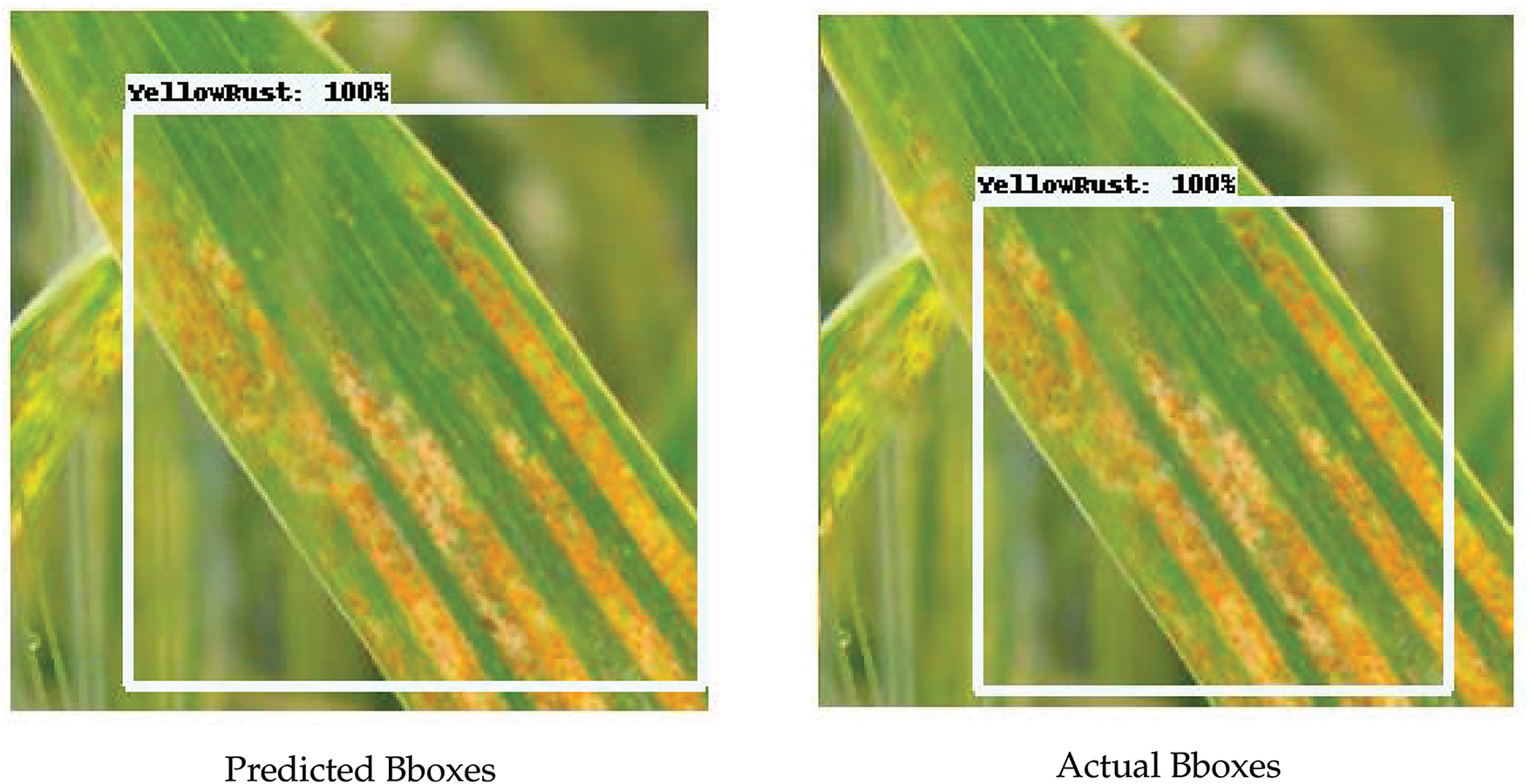
Figure 7: Single disease, i.e., yellow rust detection

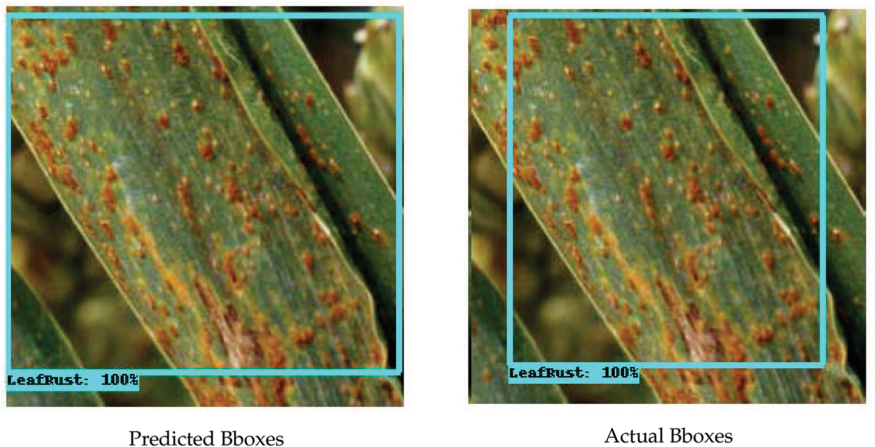
Figure 8: Detection of leaf rust disease

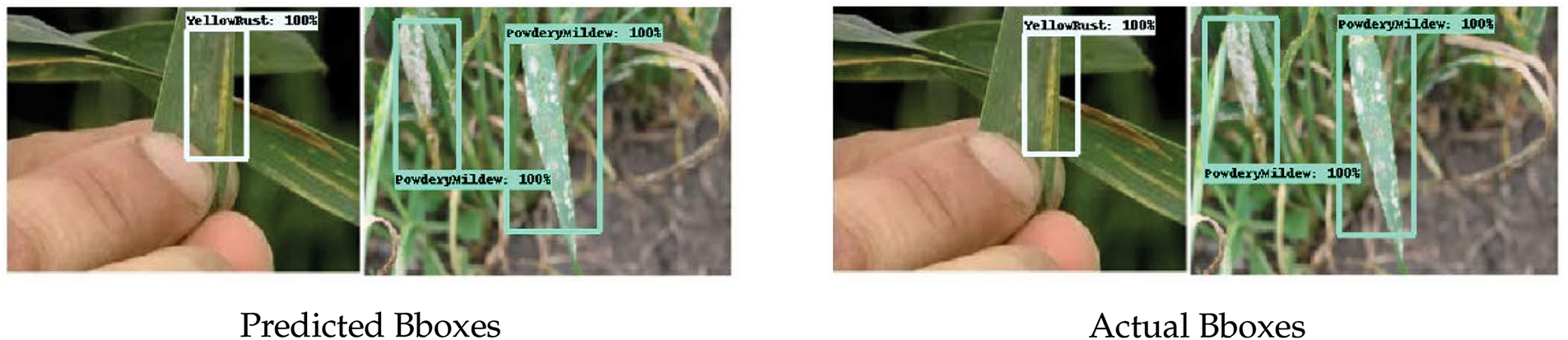
Figure 9: Multi-diseases detection of yellow rust and powdery mildew diseases

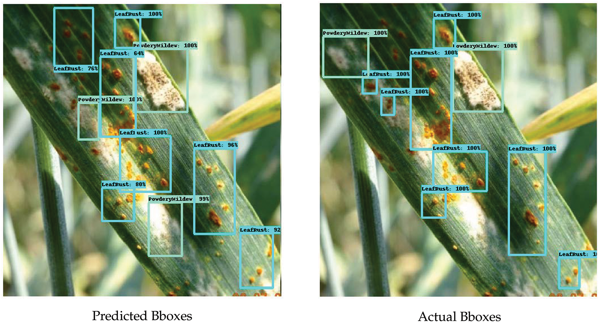
Figure 10: Detection result of leaf rust, and powdery mildew on single leaf

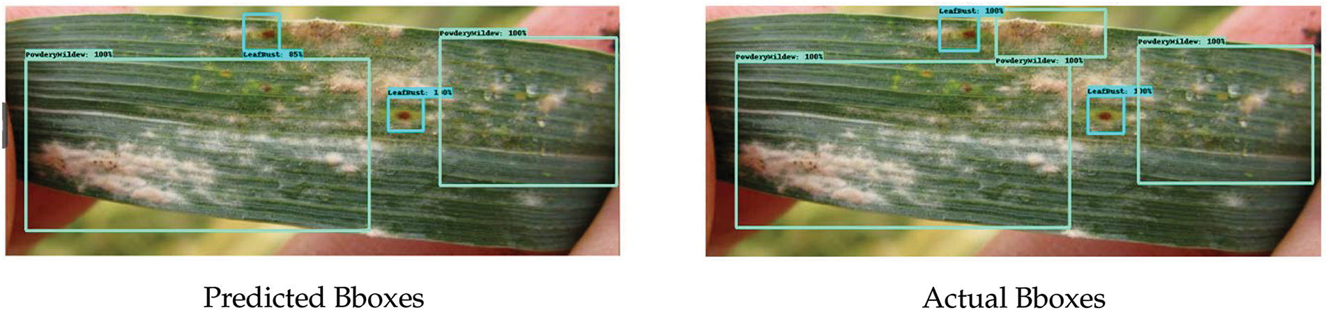
Figure 11: Multi-disease detection of leaf rust and powdery mildew disease on single leaf

4.1.6 Model Evaluation

Two manual observations were used to evaluate the model. Furthermore, to evaluate the accuracy of the model, Observation 1 compares the predicted and ground-truth bounding boxes. Observation 2 examined the detection results using different levels of confidence.

Observation 1: Accuracy evaluation

The actual and predicted bounding boxes were compared to obtain accuracy scores. The Faster R-CNN (ResNet50) model, which was trained on images with a size of 800 × 1333 and a receptive field, produced appreciable results. In this observation, only bounding boxes with a specified ground truth were considered, and those without a ground truth were ignored for comparative analysis. To determine the accuracy of the model for the test images, Table 9 lists the variances between the actual and predicted anchor boxes. All the images were examined to identify various diseases.

A single disease may be observed in some of these images, whereas numerous disease symptoms can be observed in others. For example, in the case of leaf rust disease, the model correctly identified five of eight bounding boxes; however, a few images showed similar symptoms for both leaf rust and powdery mildew. In contrast, for powdery mildew, the model correctly predicted three of the four boundary boxes. This means that the model can predict real bounding boxes with an accuracy of 85.85%.

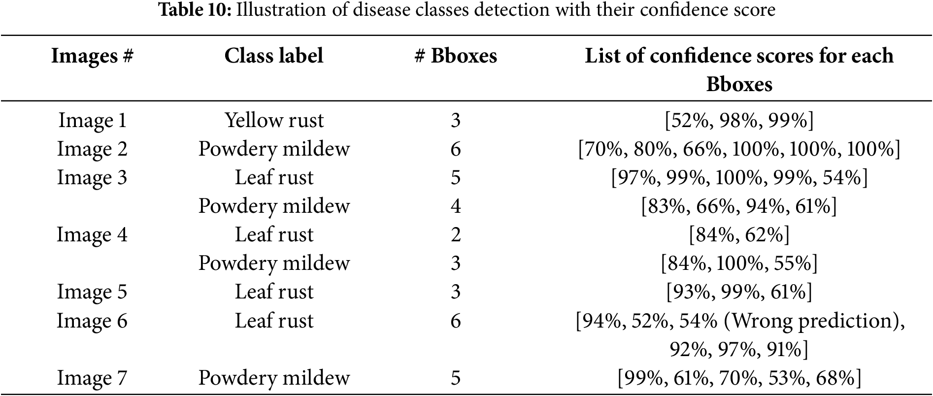
Observation 2: Model evaluation from the confidence score

Confidence scores were used to evaluate model performance. The IoU value was used to compute the confidence score prediction. Here, the model predicts bounding boxes with a confidence score higher than 50%, and ignores the remaining bounding boxes with a confidence score lower than 50%. The intersection over union (IoU) threshold is set to 0.5 for predicting the bounding boxes. Random images are used to detect different diseases, as listed in Table 10 along with the corresponding confidence scores. The model correctly predicted the class label, with a maximum confidence value of 70%. Nevertheless, in certain cases, the model continues to expect a proper class label, even when the confidence level drops below 70%. However, in some instances, the model predicted the class label inaccurately with a lower confidence score; one such example was misclassified as leaf rust with a confidence score of 54%. Therefore, choosing an IoU threshold value of 0.5 is the best option for identifying various fungal infections in wheat crops.

4.2 Wheat Disease Detection Using YOLOv8

YOLOv8, designed by Ultralytics, is an advanced technique that combines instance segmentation, image classification, and object recognition to identify crop diseases instantly. YOLOv8, which builds on the popular YOLO series, particularly YOLOv5, significantly improves the accuracy and efficiency of computer vision tasks. Projects that take advantage of an intuitive Python package and command-line interface backed by a strong professional community have illustrated its adaptability [37,38]. YOLOv8 provides several architectural enhancements compared with YOLOv5 by emphasizing its accuracy, efficiency, and adaptability. Substituting a reduced, reparameterized backbone for the CSPDarknet53 backbone improves speed and feature extraction. The PANet neck was transformed into an Enhanced Path Aggregation Network (EPAN) with dynamic routing and spatial attention to further enhance the feature fusion. The bounding box prediction was simplified and the computational overhead was decreased by YOLOv8’s anchor-free architecture. Its adjustable decoupling head and dynamic loss function maximize the performance of certain tasks. Additionally, by adding support for segmentation and keypoint detection tasks, YOLOv8 expands its capabilities beyond object detection [39,40]. To improve the efficiency and accuracy, YOLOv8 uses an anchor-free detection technique that directly predicts the object centers. The model’s use of mosaic augmentation during training further demonstrated its adherence to innovation. By exposing the model to various situations, this method promotes a thorough learning [41]. In mosaic augmentation, four distinct images are arranged in a 2 × 2 grid to form a single mosaic image. A single image was created by randomly cropping and scaling portions of each image. Mosaic augmentation combines numerous images into various training samples, thereby improving small-object representation, context understanding, data efficiency, and model generalization. The YOLOv8 model was a perfect fit for our research project because of its substantial architectural improvements, which included a superior feature pyramid network, adaptive anchor calculation, and an advanced loss function. These enhancements significantly accelerate the inference times and increase the detection accuracy, making it well suited to our research. The increased accuracy and efficiency of YOLOv8 were crucial for our investigation, which required high-speed processing and accurate detection in situations that changed quickly.

4.2.1 Model Architecture

YOLO is a state-of-the-art object detection technique that is widely accepted in computer vision owing to its speed of detection. YOLOv8, the most recent version of the architecture of the model, is given in Fig. 12, the YOLO architecture was initially presented in the C programming language, and its repository, DarkNet, was continuously maintained by its developer, Joseph Redmond, while pursuing his doctorate at the University of Washington. The YOLOv3 version of PyTorch, developed by Glenn Joffker, indicated the beginning of an amazing advancement in object identification. He created the YOLOv3 PyTorch repository to replicate YOLOv3 from DarkNet, but it soon exceeded these goals. Consequently, his business, ultralytics, released YOLOv5, which increased the popularity and accessibility of the model among developers. Different models started to appear as the excitement increased. Scaled YOLOv4 and YOLOv7 are notable branches of the YOLOv5 repository. Furthermore, independent models such as YOLOx and YOLOv6 demonstrate the creative capacity of the community. Ultralytics confirms its role in advancing AI-driven solutions by continuing to maintain the YOLOv5 repository, which is an essential resource for the object detection community.

Figure 12: Basic architecture of YOLOv8 [41]

YOLOv8, one of the most recent YOLO (You Only Look Once) models, represents a breakthrough in object identification. YOLOv8, which Ultralytics has been working on over the last six months, offers significant architectural improvements. For efficient object detection, the YOLO core integrates features through a neck and analyzes image pixels at different resolutions by using a backbone of convolutional layers. By predicting the centers of objects directly, YOLOv8’s anchor-free architecture overcomes the problems with anchor boxes that plagued earlier iterations. Traditional models concentrate on class loss and the loss of objectness. By streamlining the detection process, this anchor-free method increases the efficiency and accuracy. With these enhancements, YOLOv8 represents a groundbreaking solution for object detection. Fig. 13 shows some glimpses during the model-training process.

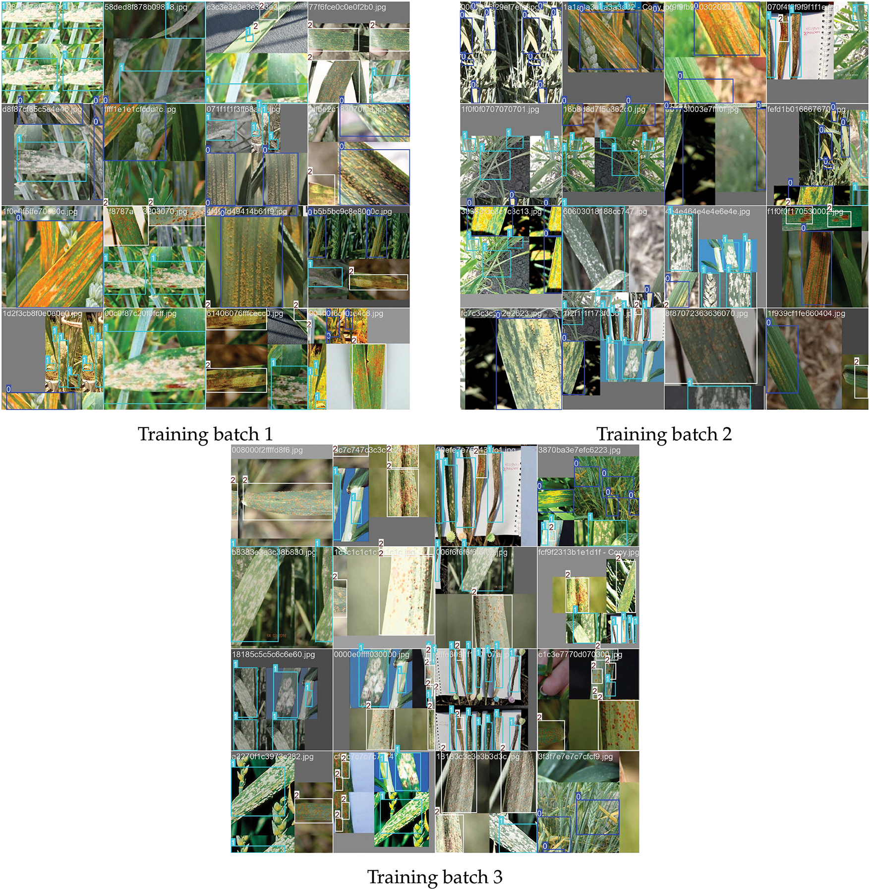
Figure 13: Training glimpses on different batches

4.2.2 Training the Model

Table 11 lists the training results of the YOLOv8 model for the different epochs. In addition, Google Collab Pro was used to train the model. A total of 355 images, comprising 50 images of mixed diseases and 100 images for each class–leaf rust, yellow rust, and powdery mildew–were used to train the YOLOv8 model. Seven distinct epoch settings (200, 400, 600, 700, 800, 1000, and 1200 epochs) were used to train the models. Mean average precision (mAP), training time, and inference speed per image (measured in milliseconds) were used to assess model performance. A performance study of the YOLOv8 model over a range of epochs showed that as the number of training epochs increased, the mean average precision (mAP) consistently improved. With additional training epochs, the mAP of the model increased from 0.502 at 200 epochs to 0.926 at 1200 epochs, indicating an improved capacity to learn intricate patterns. The 200–400 epoch range (0.502–0.753) saw the largest gains in mAP, suggesting a quick learning phase in the early stages of training. However, after 600 epochs, the pace of progress decreased, and moderate advances were observed between 700 and 1000 epochs. Unexpectedly, only a small mAP improvement (from 0.907 to 0.926) was obtained when the number of epochs increased from 1000 to 1200, indicating a reduction in gains with additional training.

The training time increased with the number of epochs, from 1.861 h for 200 epochs to 9.471 h for 1000 epochs. However, at 1200 epochs, the training time surprisingly dropped to 2.422 h; the reason might be that the model may have undergone optimization during its convergence process. With values between 0.2 and 0.3 ms per image, the inference speed remained constant across all epoch settings, demonstrating that extended training did not affect the model’s capacity to detect objects in real time. According to these results, training for a larger number of epochs improves accuracy; however, performance gains over 1000 epochs are negligible, and training for 1200 epochs requires less time, which may be the best compromise between computational efficiency and accuracy.

Training Time and Speed Analysis: With the notable exception of a drop at 1200 epochs, where the training time was significantly reduced at 2.422 h compared to 9.471 h for 1000 epochs, the training times generally increased with additional epochs. This implies that the training process was optimized at higher epochs, regardless of the hardware efficiency or early convergence. Moreover, for every image, the inference speed varied between 0.2 and 0.3 ms, staying comparatively constant across all epoch settings. This consistency indicates that the prediction speed did not decrease as model accuracy and complexity increased. Interestingly, the training time decreased significantly to 2.422 h, even though the mAP improved at 1200 epochs. Hardware or model optimization, such as early stopping or a faster rate of convergence, could be the cause of this odd behavior. Despite this, the performance and efficiency of the 1200-epoch model were the best, indicating that it might be the ideal configuration.

Model Accuracy vs. Epochs: At 200 epochs, the mAP value was 0.502; at 1200 epochs, it improved significantly to 0.926. The mAP improved from 0.845 to 0.907 between 600 and 1000 epochs and between 200 and 400 epochs, and it rose from 0.502 to 0.753. These are the two most notable advances in the field. The improvements were less significant, with the mAP increasing from 0.907 to 0.926 during the 1000 and 1200 epochs. This implies that while longer training sessions can result in improved performance, the benefits decrease as the number of epochs increases beyond 1000. All epochs exhibited a constant inference speed, which is essential for real-time detection. The model operated with remarkable efficiency, averaging between 0.2 and 0.3 ms per image. This indicates that even as the number of training epochs and mAP increases, the YOLOv8 model maintains its speed. Fig. 14 shows the code snippet used to train the model on the best-trained parameters.

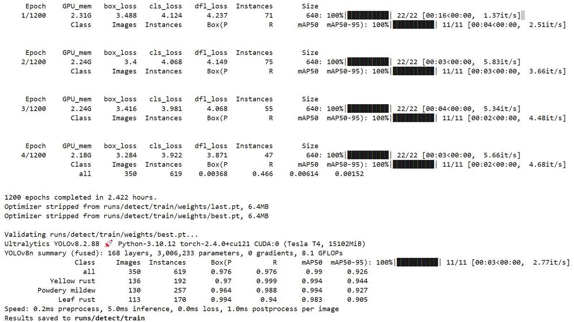
Figure 14: Code snippet of training the YOLOv8 model

Optimal Epoch Selection: Training for 600−800 epochs would probably provide an optimal compromise between training time (5.580–7.002 h) and performance (mAP ∼ 0.845–0.881) for the majority of applications. However, training for 1000 epochs (mAP = 0.907) or 1200 epochs (mAP = 0.926) could make sense for crucial jobs in which maximal accuracy is required. With the maximum mean average precision (mAP) attained at 1200 epochs, the YOLOv8 model showed consistent performance gains across all epoch settings. The constant inference speed of the model, along with the significant reduction in the training time at 1200 epochs, indicates that this is the most efficient setting overall. However, 600–800 epochs offer a fair compromise between near-optimal accuracy and reduced processing demands for applications where the training time is more important. Early Stopping: When the accuracy reaches equilibrium at higher epochs, implementing early stopping criteria may help to further optimize the training time. Generalization: The ability of the model to adapt to previously unidentified cases may be enhanced by growing the dataset or employing data augmentation strategies. Hardware Optimization: Given the dramatic drop in training times at 1200 epochs, it is possible to investigate additional hardware optimizations or adaptive training techniques to reduce the training times for each epoch.

4.2.3 Results and Discussion

Furthermore, to estimate the performance of the YOLOv8 model, we used several performance measures, such as the confusion matrix and PR curve.

Confusion Matrix: This is a square matrix that provides a clear view of the correctly predicted samples from the incorrectly predicted samples for each class. Fig. 15 shows a comparison of the confusion matrix results for the three most frequent epochs: 800, 1000, and 1200. The model consistently performs well for Yellow rust and Powdery mildew, with Yellow rust improving from 0.99 to 1.00 and Powdery mildew staying stable at 0.99 throughout, according to the confusion matrix results throughout 800, 1000, and 1200 epochs. Compared to other materials, leaf rust shows greater fluctuation, with an initial value of 0.95 decreasing to 0.94 at 1000 epochs, and then improving to 0.96 by 1200 epochs. This shows that yellow rust and powdery mildew were successfully classified by the model at an early stage; however, leaf rust requires additional training to perform at its best, most likely because of the complexity of its features. With some potential for a small improvement in leaf rust, the model demonstrated a good classification accuracy for all three classes by the end of 1200 epochs.

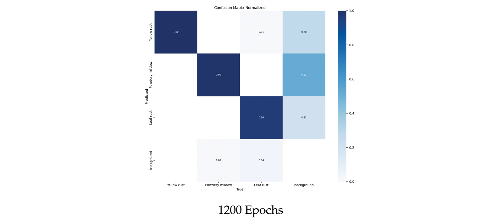
Figure 15: Confusion matrix results on different epochs

Precision-Recall Curve: The model’s increasing performance with more training is shown by the precision-recall results for the 800, 1000, and 1200 epochs of yellow rust, powdery mildew, and leaf rust classifications, as depicted in Fig. 16. The precision-recall values for yellow rust were consistently high, beginning at 0.993 at 800 epochs and slightly increasing to 0.994 at 1200 epochs. This suggests that the model can correctly categorize the disease even in its early stages. Similarly, powdery mildew showed consistently high performance; during the epochs, precision-recall values increased from 0.992 to 0.994, indicating how easily the model could discriminate this class. Leaf rust, on the other hand, started with a lower precision-recall value of 0.968 at 800 epochs but then dramatically improved to 0.983 by 1200 epochs. This shows that leaf rust is more complex than other diseases, either because of overlapping traits or imbalances between classes. Consequently, the model required more training to properly classify leaf rust. The consistent enhancement over the epochs indicates that the model is gradually gaining proficiency in managing leaf rot. Along with this epoch-to-epoch growth, the mean average precision (mAP) began at 0.984 at 800 epochs, increased to 0.987 at 1000 epochs, and reached 0.990 at 1200 epochs. This indicates a steady improvement in the capacity of the model to strike a balance between recall and precision throughout the training for all classes, particularly the more difficult leaf rust disease class. These findings indicate that although the model performs exceptionally well in the early stages of powdery mildew and yellow rust, more training greatly improves the model’s ability to classify leaf rust and the overall performance. Hence, for 1200 epochs, the YOLOv8 model performed well. Therefore, we analyzed the loss graph comparison by fixing the results for 1200 epochs. In object detection, a loss graph is useful for analyzing the learning process, detecting overfitting and underfitting problems, and determining whether a model has reached convergence. The convergence point was defined as the moment at which the training and validation losses decreased significantly. This indicates that additional training may not result in any improvement because the model has learned as much as possible using its current configuration. Fig. 17 shows the training and validation loss graph results, where we can clearly see that a smooth curve has been obtained for both the training and validation data. However, a smoother curve has obtained for the validation data.

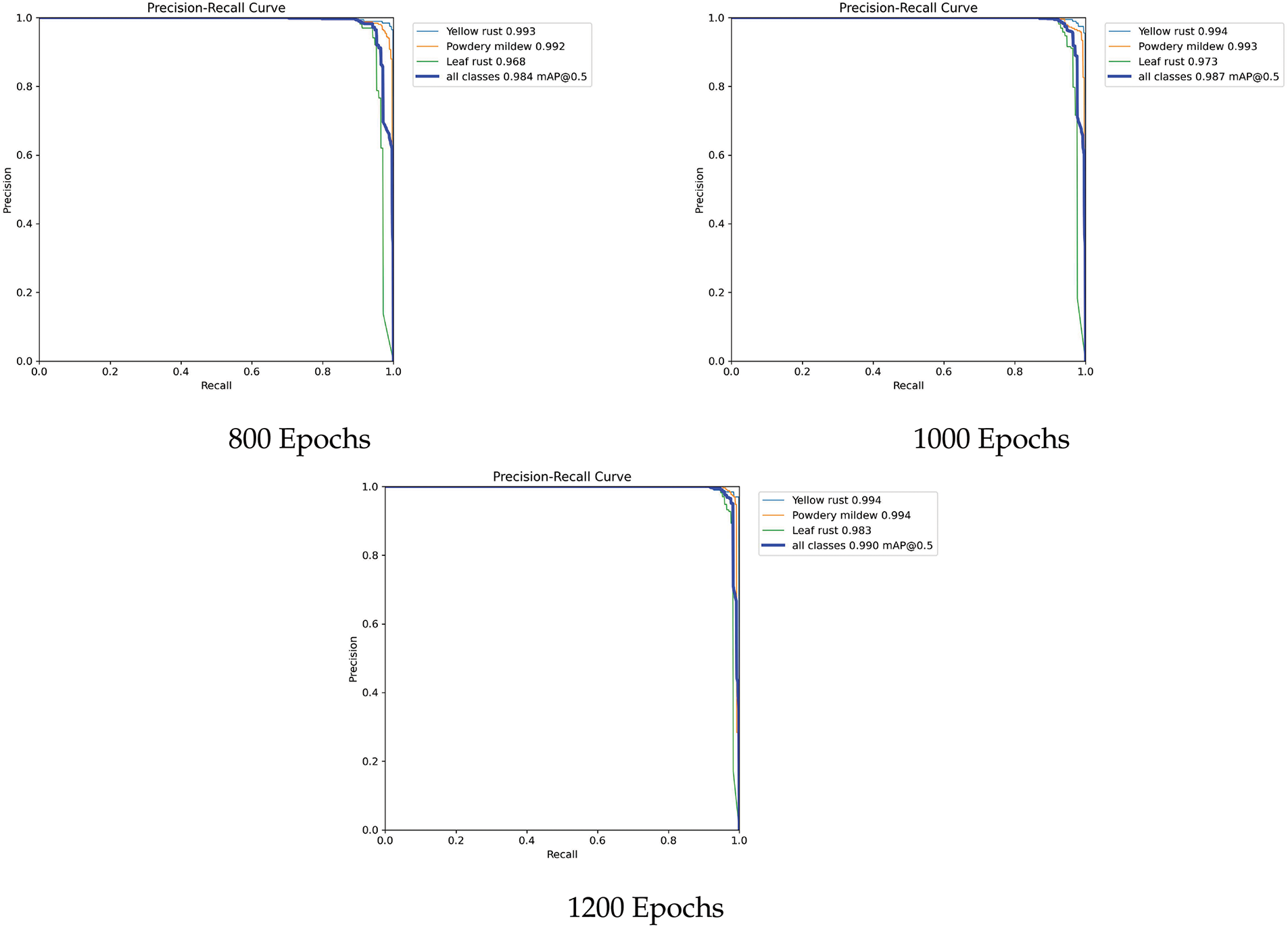
Figure 16: Precision recall curve results on various epochs

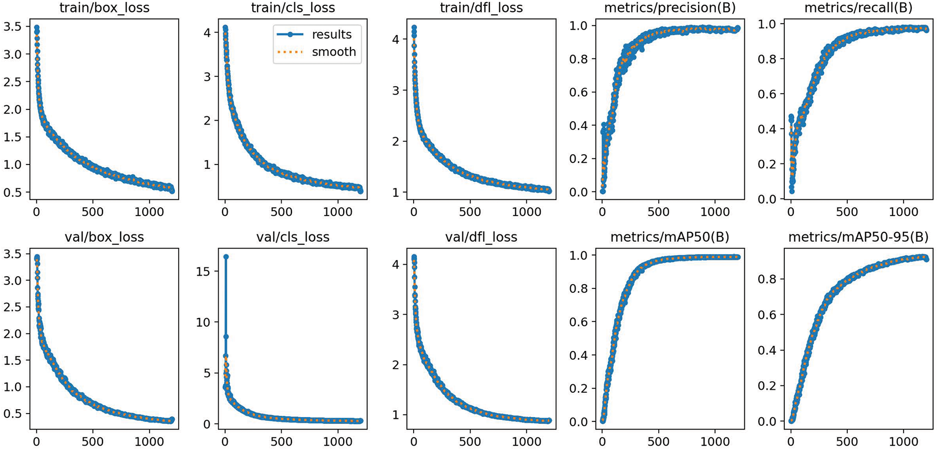
Figure 17: Training and validation loss graph comparison

Further, Figs. 18–20 show the detection results of the YOLOv8 model for all classes, i.e., yellow rust, powdery mildew, and leaf rust diseases for 1200 epochs. Object detection models are used to detect plant diseases such as yellow rust, powdery mildew, and leaf rust. The prediction accuracy of the model is indicated by confidence scores, bounding boxes around the infected areas, and class labels that identify a specific disease. For example, a bounding box may enclose a leaf area that exhibits symptoms of leaf rust or yellow rust. A class label, such as “yellow rust,” “powdery mildew,” or “leaf rust,” is issued to each bounding box based on the particular traits that the model finds. For instance, yellow-orange pustules may indicate the presence of powdery mildew, which appears as a white powdery substance on the leaf surface, and reddish-brown patches may indicate the presence of leaf rust. The algorithm yields a confidence score that indicates the degree of certainty that the diagnosed disease is leaf rust, powdery mildew, or yellow rust in addition to the class designation. The model is quite definite in its classification if it has a high confidence level (e.g., 0.90% or 90%), whereas a lower value indicates less confidence. For instance, if a detected area has a bounding box labeled “yellow rust” and an 85% confidence level, the model may have 85% confidence that yellow rust affects the leaf section inside the box. Similarly, the model is slightly less convinced but still believes that the detected region includes powdery mildew if another box is labeled “powdery mildew” with a confidence score of 0.75.

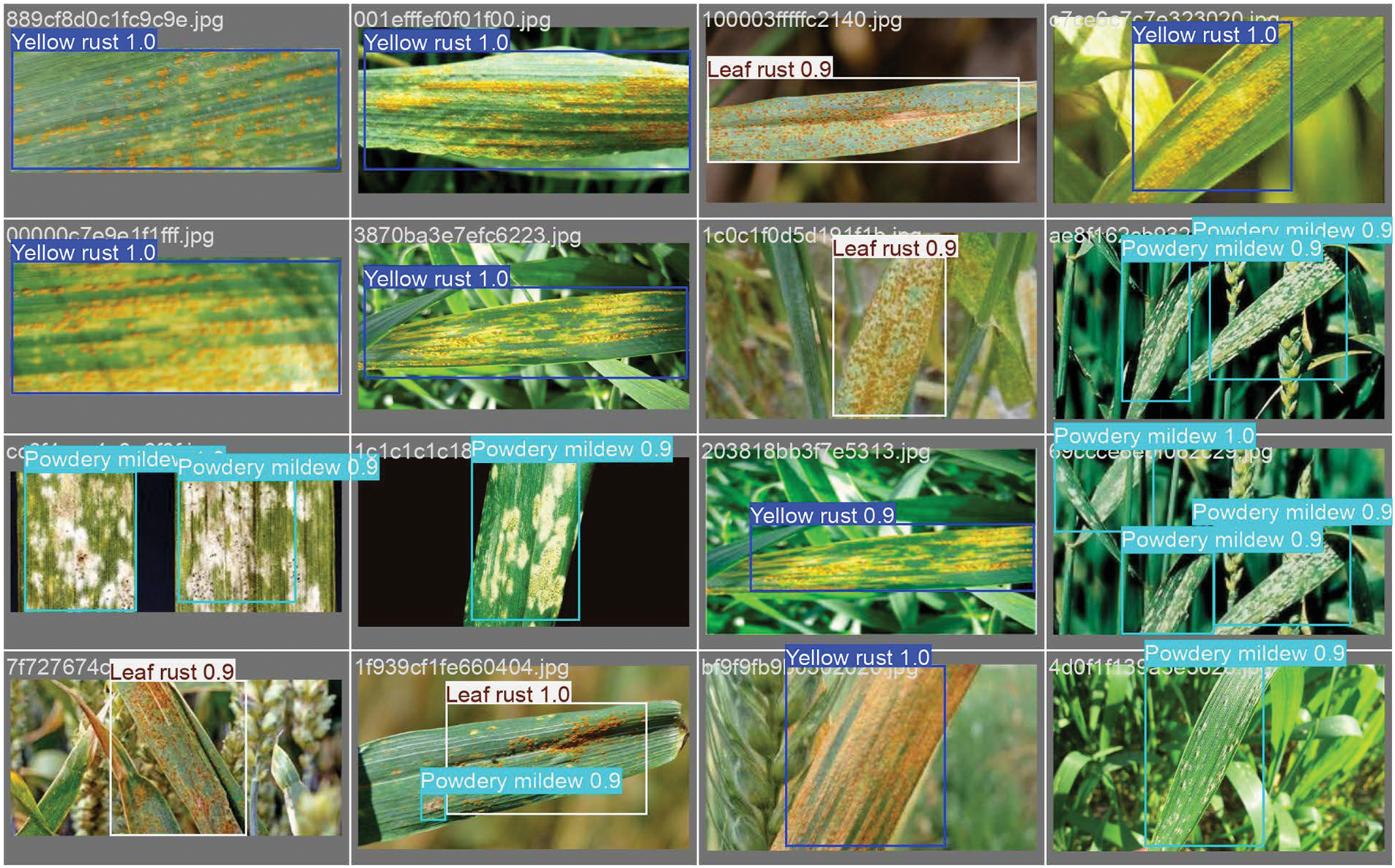
Figure 18: Detection results on validation batch 1

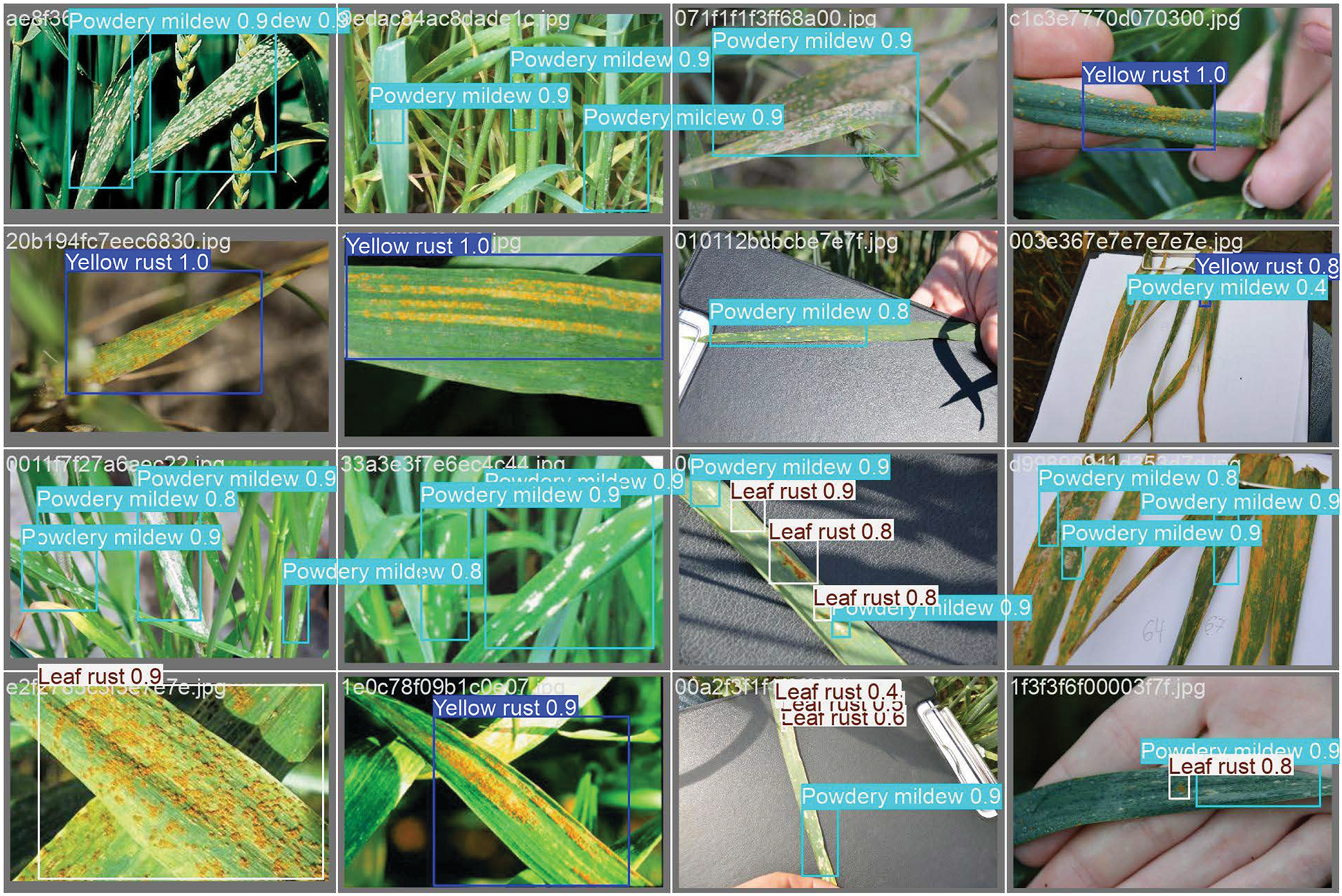
Figure 19: Detection results on validation batch 2

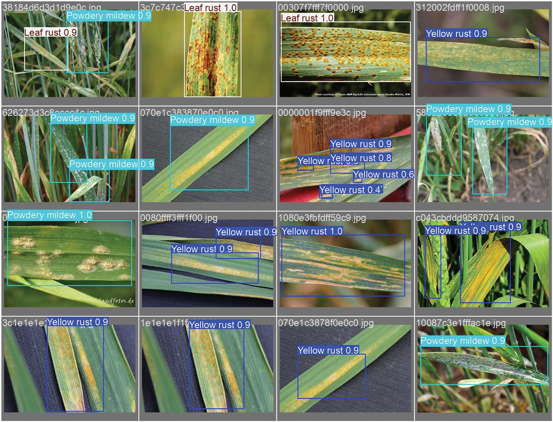
Figure 20: Detection results on validation batch 3

4.3 Comparative Study on Faster R-CNN and YOLOv8 Model

The TensorFlow Faster R-CNN object identification model may not provide the same mean average precision (mAP) as the YOLOv8 model for several reasons. The mean average precision of the YOLOv8 model is higher than that of TensorFlow R-CNN because of its sophisticated training methodology, anchor-free design, end-to-end learning, enhanced feature extraction, and efficient post-processing. These characteristics lead to improved object localization and classification, faster model convergence, and improved generalization for small and diverse objects. Although Faster R-CNN is more accurate in certain scenarios, its mAP is lower in some cases because it is generally slower and less efficient when handling particular object scales and complexities. YOLOv8 incorporates advanced techniques, such as deeper layers, stronger loss functions, and enhanced feature fusion algorithms (such as PANet and CSPDarknet) to achieve more generalization. Owing to these enhancements, YOLOv8 can now recognize objects more accurately over a wider variety of scales and settings, improving its performance for small and crowded items. Faster R-CNN usually has trouble recognizing small objects and complex backdrops because it relies on area recommendations, which may not capture small or partially veiled items accurately. The enhanced performance of YOLOv8 is a result of the following factors:

End-to-End Learning in YOLOv8: YOLOv8 is a single-stage, end-to-end solution. Instantly, anticipating bounding boxes and class probabilities from the input image improves the overall detection pipeline. Conversely, the faster R-CNN uses a two-stage detector. It generates region proposals using a Region Proposal Network (RPN) and then classifies these areas.

Anchor-Free Design in YOLOv8: YOLOv8’s anchor-free architecture eliminates the requirement for anchor boxes by anticipating object centers and bounding boxes. This makes object localization easier. This increases the object localization accuracy and reduces errors, particularly for objects that do not fit tightly within the designated anchor forms. However, disparities between anchor boxes and actual objects may result from the use of anchor-based detection by a faster R-CNN, especially when objects have significant scale or aspect ratio fluctuations. This may result in a decrease in the mAP, particularly in datasets that include a variety of object sizes.

Advanced Post-Processing Techniques: YOLOv8 uses two advanced post-processing techniques to improve precision by reducing false positives and reinforcing the model’s tolerance to changing input sizes: non-maximum suppression (NMS) and multiscale training. Even with the addition of NMS, Faster R-CNN’s two-stage method sometimes yields less-than-optimal region recommendations, lowering the mAP and compromising the overall accuracy, particularly if the area proposals miss important objects.

Improved Feature Extraction and Architecture in YOLOv8: YOLOv8 can gather more comprehensive features across sizes owing to its enhanced feature pyramids and more intricate backbone architecture (such as CSPDarknet). A higher mAP is the result of improved item recognition and categorization ability. Even though it is more powerful, the Faster R-CNN architecture might not gain from the same degree of architectural optimization, and its feature extraction network might not be as effective as the core of YOLOv8 in extracting multi-scale features.

Loss Function and Training Strategy: The advanced loss function of YOLOv8 achieves a balance between objectness, classification, and bounding box regression losses. This ensured that the model was calibrated precisely, highlighting the accuracy of object detection and decreasing the overlap between the anticipated boxes. A faster R-CNN uses different losses to classify objects and produce region proposals. When these losses are split apart, the total mAP may be reduced, which may lead to erroneous classifications or less ideal placement of the bounding box.

Data Augmentation and Regularization: Improved data augmentation techniques (including threshold, random scaling, and mosaic augmentation) are frequently incorporated into YOLOv8 training, which improves the mAP and aids in the adaptation of the model to new data. Data augmentation is possible with TensorFlow Faster R-CNN; however, by default, it may not be applied as an aggressive or diverse augmentation technique, which could result in a lower mAP and worse generalization performance.

Hardware Utilization and Optimization: YOLOv8’s design incorporates batch normalization and other performance-enhancing changes to enable it to operate more quickly and effectively on contemporary technologies, such as GPUs and specialized edge devices. Despite its versatility, TensorFlow Faster R-CNNs may result in less-than-ideal weight updates and delayed training, which could negatively impact model performance at the final mAP.

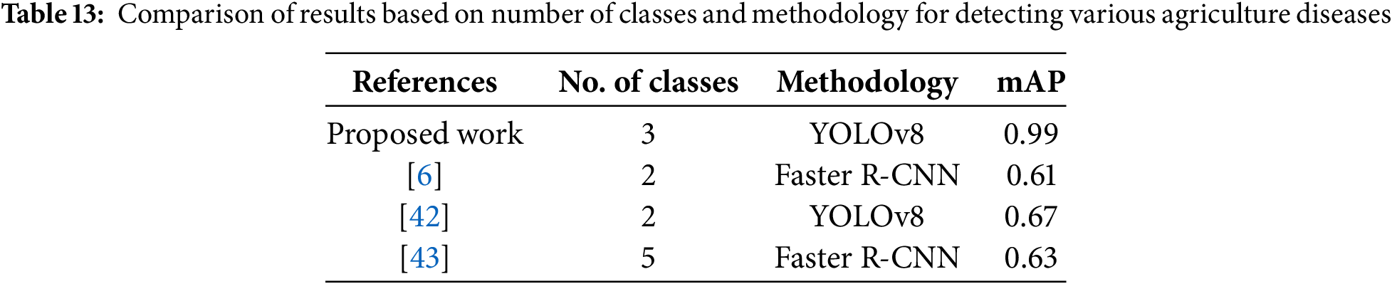
Computer-vision-based deep-learning models have recently made significant progress in plant disease identification. Many pretrained object identification models that require less time and effort to train are available, making them ideal for addressing domain-specific problems in industries such as healthcare and agriculture. This reduces the training time and the computational cost. Tables 12 and 13 present a comparison of the results obtained with the proposed method and other models along with state-of-the-art techniques, respectively. With YOLOv8, Faster R-CNN, and the proposed framework tested under identical circumstances, the comparison demonstrates the effectiveness of various object detection algorithms. The performance measures of YOLOv8 (0.67) and Faster R-CNN (0.63 and 0.61), as reported in other studies, show competitive but unsatisfactory accuracy in difficult situations. However, our model showed a significant gain, attaining a YOLOv8 performance measure of 0.99, highlighting its ability to use significant optimizations and architectural improvements to provide better detection accuracy. This enhancement highlights how well our strategy addresses the shortcomings of the current models. A comparative analysis revealed that the proposed the TensorFlow-based fine-tuning model, Faster R-CNN with ResNet50 backbone model, produced higher mean average precision findings than the state-of-the-art models. On the other hand, the Pytorch-based YOLOv8 the model revealed the maximum mean average precision of 0.99 for detecting and classifying multiple wheat fungal diseases. The YOLOV8 model is the best choice over other state-of-the-art algorithms for detecting agricultural diseases. The findings of this study contribute significantly to the existing body of knowledge by providing new insights into the agriculture field. The system was tested under diverse real-world scenarios to validate its practicality and reliability.

5  Conclusions and Future Directions

With a focus on leaf rust, yellow rust, and powdery mildew, this study used one- and two-stage object detection models to identify and classify fungal infections in wheat. Starting with TensorFlow-based models, the WFD2020 dataset–which is available at “http://wfd.sysbio.ru/”–was used to modify the model parameters to improve detection accuracy. The Faster R-CNN-based model with the backbone ResNet50 yielded the greatest mAP results at 0.68. In addition, the accuracy of the model was confirmed by manual observations, yielding a high confidence score for bounding box predictions. The optimized Faster R-CNN model, with an accuracy rate of 85.85%, was obtained from manual observations. Following this, the PyTorch-based YOLOv8 model achieved a remarkable mAP of 0.99 for each of the three disease classes during model training. However, these issues remain in certain circumstances, particularly when there is uneven light distribution and little distinction between various disease categories. Without addressing the shortcomings of the study, including its small dataset size, lack of diversity in disease classifications, and inconsistent mAP values, the conclusions minimized the study’s contributions. To overcome these limitations, future research options include expanding the dataset to include additional images captured under various lighting conditions. Additionally, quantifying the number of pathogenic spores in wheat crops could enhance the assessment of infection severity. In addition, the potential use of web or mobile applications seems to be an intriguing approach for on-site fungal disease detection in wheat fields. Farmers may be able to prevent the spread of diseases and safeguard agricultural output using such technology, which would provide them with real-time knowledge and enable them to act quickly.

Acknowledgement: This research is supported by Princess Nourah bint Abdulrahman University Researchers Supporting Project number (PNURSP2025R432), Princess Nourah bint Abdulrahman University, Riyadh, Saudi Arabia.

Funding Statement: This research is supported by Princess Nourah bint Abdulrahman University Researchers Supporting Project number (PNURSP2025R432), Princess Nourah bint Abdulrahman University, Riyadh, Saudi Arabia.

Author Contributions: Shivani Sood: Conceptualization, Methodology, Software, Investigation, Writing—original draft preparation. Harjeet Singh: Conceptualization, Investigation, Writing—review and editing. Surbhi Bhatia Khan: Conceptualization, Investigation, Writing—review and editing. Ahlam Almusharraf: Conceptualization, Investigation, Writing—review and editing, Supervision. All authors reviewed the results and approved the final version of the manuscript.

Availability of Data and Materials: Dataset used in this study can be download from “http://wfd.sysbio.ru/”.

Ethics Approval: Data confidentiality and anonymity were maintained throughout the research process.

Conflicts of Interest: The authors declare no conflicts of interest to report regarding the present study.

References

1. Curtis BC, Rajaram S, Gómez Macpherson H. Bread wheat: improvement and production. Rome, Italy: Food and Agriculture Organization of the United Nations; 2002. [Google Scholar]

2. Azimi N, Sofalian O, Davari M, Asghari A, Zare N. Statistical and machine learning-based fhb detection in durum wheat. Plant Breed Biotech. 2020;8(3):265–80. doi:10.9787/pbb.2020.8.3.265. [Google Scholar] [CrossRef]

3. Roelfs AP, Singh RP, Saari E. Rust diseases of wheat: concepts and methods of disease management. Mexico: Cimmyt; 1992. [cited 2025 Jan 20]. Available from: https://rusttracker.cimmyt.org/wp-content/uploads/2011/11/rustdiseases.pdf. [Google Scholar]

4. Panhwar QA, Ali A, Naher UA, Memon MY. Fertilizer management strategies for enhancing nutrient use efficiency and sustainable wheat production. In: Organic farming. UK: Woodhead Publishing; 2019. p. 17–39. [Google Scholar]

5. Hasan MM, Chopin JP, Laga H, Miklavcic SJ. Detection and analysis of wheat spikes using convolutional neural networks. Plant Methods. 2018;14(1):1–13. doi:10.1186/s13007-019-0405-0. [Google Scholar] [CrossRef]

6. Liu H, Jiao L, Wang R, Xie C, Du J, Chen H, et al. WSRD-Net: a convolutional neural network-based arbitrary-oriented wheat stripe rust detection method. Front Plant Sci. 2022;13:876069. doi:10.3389/fpls.2022.876069. [Google Scholar] [PubMed] [CrossRef]

7. Lin Z, Mu S, Huang F, Mateen KA, Wang M, Gao W, et al. A unified matrix-based convolutional neural network for fine-grained image classification of wheat leaf diseases. IEEE Access. 2019;7:11570–90. doi:10.1109/access.2019.2891739. [Google Scholar] [CrossRef]

8. Picon A, Alvarez-Gila A, Seitz M, Ortiz-Barredo A, Echazarra J, Johannes A. Deep convolutional neural networks for mobile capture device-based crop disease classification in the wild. Comput Electr Agricult. 2019;161:280–90. doi:10.1016/j.compag.2018.04.002. [Google Scholar] [CrossRef]

9. Dong M, Mu S, Shi A, Mu W, Sun W. Novel method for identifying wheat leaf disease images based on differential amplification convolutional neural network. Int J AgricultBiolog Eng. 2020;13(4):205–10. doi:10.25165/j.ijabe.20201304.4826. [Google Scholar] [CrossRef]

10. Mohanty SP, Hughes DP, Salathé M. Using deep learning for image-based plant disease detection. Front Plant Sci. 2016;7:215232. doi:10.3389/fpls.2016.01419. [Google Scholar] [PubMed] [CrossRef]

11. Liu B, Zhang Y, He D, Li Y. Identification of apple leaf diseases based on deep convolutional neural networks. Symmetry. 2017;10(1):11 doi: 10.3389/fpls.2021.723294. [Google Scholar] [PubMed] [CrossRef]

12. Ferentinos KP. Deep learning models for plant disease detection and diagnosis. Comput Electr Agricult. 2018;145(6):311–8. doi:10.1016/j.compag.2018.01.009. [Google Scholar] [CrossRef]

13. Kaur S, Pandey S, Goel S. Plants disease identification and classification through leaf images: a survey. Arch Computat Meth Eng. 2019;26(2):507–30. doi:10.1007/s11831-018-9255-6. [Google Scholar] [CrossRef]

14. Sood S, Singh H. An implementation and analysis of deep learning models for the detection of wheat rust disease. In: 2020 3rd International Conference on Intelligent Sustainable Systems (ICISS); 2020 Dec 3; IEEE. p. 341–7. [Google Scholar]

15. Bravo C, Moshou D, West J, McCartney A, Ramon H. Early disease detection in wheat fields using spectral reflectance. Biosyst Eng. 2003;84(2):137–45. doi:10.1016/s1537-5110(02)00269-6. [Google Scholar] [CrossRef]

16. Moshou D, Bravo C, West J, Wahlen S, McCartney A, Ramon H. Automatic detection of ‘yellow rust’ in wheat using reflectance measurements and neural networks. Comput Electr Agricult. 2004;44(3):173–88. doi:10.1016/j.compag.2004.04.003. [Google Scholar] [CrossRef]

17. Siricharoen P, Scotney B, Morrow P, Parr G. Automated wheat disease classification under controlled and uncontrolled image acquisition. In: Image Analysis and Recognition: 12th International Conference, ICIAR 2015; 2015 Jul 22–24. Niagara Falls, ON, Canada: Springer; 2015. p. 456–64. [Google Scholar]

18. Shafi U, Mumtaz R, Qureshi MDM, Mahmood Z, Tanveer SK, Haq IU, et al. Embedded AI for wheat yellow rust infection type classification. IEEE Access. 2023;11:23726–38. doi:10.1109/access.2023.3254430. [Google Scholar] [CrossRef]

19. Zhang X, Han L, Dong Y, Shi Y, Huang W, Han L, et al. A deep learning-based approach for automated yellow rust disease detection from high-resolution hyperspectral UAV images. Remote Sens. 2019;11(13):1554. doi:10.3390/rs11131554. [Google Scholar] [CrossRef]

20. Jahan N, Flores P, Liu Z, Friskop A, Mathew JJ, Zhang Z. Detecting and distinguishing wheat diseases using image processing and machine learning algorithms. In: 2020 ASABE Annual International Virtual Meeting; 2020; St. Joseph, Michigan: American Society of Agricultural and Biological Engineers. [cited 2025 Jan 20]. Available from: www.asabe.org. [Google Scholar]

21. Bao W, Zhao J, Hu G, Zhang D, Huang L, Liang D. Identification of wheat leaf diseases and their severity based on elliptical-maximum margin criterion metric learning. Sustain Comput: Inform Syst. 2021;30(1):100526. doi:10.1016/j.suscom.2021.100526. [Google Scholar] [CrossRef]

22. Chin PW, Ng KW, Palanichamy N. Plant disease detection and classification using deep learning methods: a comparison study. J Inform Web Eng. 2024;3(1):155–68. doi:10.33093/jiwe.2024.3.1.10. [Google Scholar] [CrossRef]

23. Goyal L, Sharma CM, Singh A, Singh PK. Leaf and spike wheat disease detection & classification using an improved deep convolutional architecture. Inform Med Unlocked. 2021;25:100642. doi:10.1016/j.imu.2021.100642. [Google Scholar] [CrossRef]

24. Hayit T, Erbay H, Varçın F, Hayit F, Akci N. Determination of the severity level of yellow rust disease in wheat by using convolutional neural networks. J Plant Pathol. 2021;103(3):923–34. doi:10.1007/s42161-021-00886-2. [Google Scholar] [CrossRef]

25. Schirrmann M, Landwehr N, Giebel A, Garz A, Dammer KH. Early detection of stripe rust in winter wheat using deep residual neural networks. Front Plant Sci. 2021;12:469689. doi:10.3389/fpls.2021.469689. [Google Scholar] [PubMed] [CrossRef]

26. Li J, Li C, Fei S, Ma C, Chen W, Ding F, et al. Wheat ear recognition based on RetinaNet and transfer learning. Sensors. 2021;21(14):4845. doi:10.3390/s21144845. [Google Scholar] [PubMed] [CrossRef]

27. Genaev MA, Skolotneva ES, Gultyaeva EI, Orlova EA, Bechtold NP, Afonnikov DA. Image-based wheat fungi diseases identification by deep learning. Plants. 2021;10(8):1500. doi:10.3390/plants10081500. [Google Scholar] [PubMed] [CrossRef]

28. Russell BC, Torralba A, Murphy KP, Freeman WT. LabelMe: a database and web-based tool for image annotation. Int J Comput Vis. 2008;77(1–3):157–73. doi:10.1007/s11263-007-0090-8. [Google Scholar] [CrossRef]

29. Ren S, He K, Girshick R, Sun J. Faster R-CNN: towards real-time object detection with region proposal networks. Adv Neural Inf Process Syst. 2015;28(6):1137–49. doi:10.1109/tpami.2016.2577031. [Google Scholar] [PubMed] [CrossRef]

30. Liu W, Anguelov D, Erhan D, Szegedy C, Reed S, Fu CY, et al. SSD: single shot multibox detector. In: Computer Vision-ECCV 2016: 14th European Conference; 2016 Oct 11–14; Amsterdam, The Netherlands: Springer; 2016. p. 21–37. [Google Scholar]

31. Yaseen M. What is yolov9: an in-depth exploration of the internal features of the next-generation object detector. arXiv:2409.07813. 2024. [Google Scholar]

32. Varghese R, Sambath M. Yolov8: a novel object detection algorithm with enhanced performance and robustness. In: 2024 International Conference on Advances in Data Engineering and Intelligent Computing Systems (ADICS); 2024 Apr; IEEE. p. 1–6. [Google Scholar]

33. Kumar P, Kumar V. Exploring the frontier of object detection: a deep dive into yolov8 and the coco dataset. In: 2023 IEEE International Conference on Computer Vision and Machine Intelligence (CVMI); 2023 Dec 10; IEEE. p. 1–6. [Google Scholar]

34. Kumar Y, Kumar P. Comparative study of YOLOv8 and YOLO-NAS for agriculture application. In: 2024 11th International Conference on Signal Processing and Integrated Networks (SPIN); 2024 Mar 21; IEEE. p. 72–7. [Google Scholar]

35. Chen R, Lu H, Wang Y, Tian Q, Zhou C, Wang A, et al. High-throughput UAV-based rice panicle detection and genetic mapping of heading-date-related traits. Front Plant Sci. 2024;15:1327507. doi:10.3389/fpls.2024.1327507. [Google Scholar] [PubMed] [CrossRef]

36. Li Z, Peng C, Yu G, Zhang X, Deng Y, Sun J. DetNet: a backbone network for object detection. arXiv:1804.06215. 2018. [Google Scholar]

37. Xiao B, Nguyen M, Yan WQ. Fruit ripeness identification using YOLOv8 model. Multim Tools Applicat. 2024;83(9):28039–56. doi:10.1007/s11042-023-16570-9. [Google Scholar] [CrossRef]

38. Qadri SA, Huang NF, Wani TM, Bhat SA. Plant disease detection and segmentation using end-to-end yolov8: a comprehensive approach. In: 2023 IEEE 13th International Conference on Control System, Computing and Engineering (ICCSCE); 2023 Aug 25; IEEE. p. 155–60. [Google Scholar]

39. Thuan D. Evolution of Yolo algorithm and Yolov5: the State-of-the-Art object detention algorithm; 2021 [cited 2025 Jan 20]. Available from: https://www.theseus.fi/handle/10024/452552. [Google Scholar]

40. Sapkota R, Qureshi R, Flores-Calero M, Badgujar C, Nepal U, Poulose A, et al. Yolov10 to its genesis: a decadal and comprehensive review of the you only look once series. 2024 Jun 12 [cited 2025 Jan 20]. Available from: https://papers.ssrn.com/sol3/papers.cfm?abstract_id=4874098. [Google Scholar]

41. Talaat FM, ZainEldin H. An improved fire detection approach based on YOLO-v8 for smart cities. Neural Comput Applicat. 2023;35(28):20939–54. doi:10.1007/s00521-023-08809-1. [Google Scholar] [CrossRef]

42. Zhu R, Hao F, Ma D. Research on polygon pest-infected leaf region detection based on YOLOv8. Agriculture. 2023;13(12):2253. doi:10.3390/agriculture13122253. [Google Scholar] [CrossRef]

43. Gong X, Zhang S. A high-precision detection method of apple leaf diseases using improved faster R-CNN. Agriculture. 2023;13(2):240. doi:10.3390/agriculture13020240. [Google Scholar] [CrossRef]