Low-Complexity Hardware Architecture for Batch Normalization of CNN Training Accelerator

1  Introduction

Deep Neural Networks (DNNs) [1] have achieved superior performance in many fields, including image recognition and natural language processing. However, there are several challenges when it comes to training models: vanishing gradient [2,3], exploding gradient [3], and overfitting [4] which slow down or even destabilize the training. To solve these problems, Rectified Linear Unit (ReLU) [5], gradient clipping [6], or dropout [7] can be used. Many solutions have been proposed to alleviate these problems, but normalization is one of the most powerful techniques to speed up and stabilize deep learning.

Normalization can be used for faster training and reducing the risk of being trapped in a local optimum. It changes the distribution of the activation map to enable all the features to contribute equally. It reduces over-reliance on a particular feature. In addition, normalization matches the mean and variance of each layer’s inputs and makes weight initialization less sensitive. By virtue of this, training speed increases, and the gradient vanishing problem is resolved. Generally, Batch Normalization (BN) is applied to Deep Neural Network (DNN) training. Ioffe and Szegedy (2015) [8] demonstrated that BN can accelerate training by reducing internal covariate shift. This is frequently employed in Convolutional Neural Networks (CNNs) [9] for image processing tasks, because it helps maintain more consistent distributions of the convolutional feature maps. During convolution operations, features can vary widely in scale and dynamic range, which can slow down or even destabilize training. By normalizing these features, BN mitigates internal covariate shift and ensures more stable activations, enabling faster convergence and often leading to better overall performance. Subsequently, Santurkar et al. [10] experimentally proved that BN smooths the solution space, enabling faster and more stable training. There are many analyses about normalization [11–14] as well. Afterwards, Ioffe proposed [15] to maintain performance in mini-batch, complementing the problem of BN.

However, even though normalization improves deep learning performance [16–18], there are some challenges to implementing the training engine on hardware. For the inference, the normalization layer just conducts scaling and shifting using pre-trained parameters. On the other hand, training requires several computation steps in forward and backward propagation, increasing latency and large hardware size. One approach [19] to mitigating these challenges is to reduce precision to minimize hardware resources and optimize data access to lower latency.

All normalization techniques, like BN, layer normalization [20], instance normalization [21], and group normalization [22], commonly scale features by subtracting the mean and dividing by the standard deviation. This process can introduce additional latency because of calculating the mean and standard deviation and accessing the external memory. In addition, standard deviation requires non-linear operations, like square and square root, which incur hardware overhead. Also, in backward propagation [23], the hardware gets more complex structures and computations, including partial derivative operations, as the chain rule is applied. Especially, obtaining the gradient of the normalization layer’s input is greatly complicated due to the influence of the standard deviation’s non-linear computations.

To address the intricate hardware design, the previous works have presented the approximated normalization techniques. Banner (2018) [24] first proposed the range batch normalization (RBN), which obtains standard deviation according to the range of the input distribution based on the min-max range using the characteristics of Gaussian distribution [25]. Hereby the risk of arithmetic overflows due to the sum of squared large input can be prevented, and computing standard deviation can be approximated simply by replacing the scale parameter. With the benefit of hardware-friendliness, this research is applied to other research, Bactran (2021) [26], LightNorm (2022) [27], ACBN (2023) [28]. The basis of this method is the central limit theorem, meaning that if there is a sum of many inputs, they can expect it to be approximately a Gaussian distribution. However, as known in the logic, it is difficult to assume that it follows the Gaussian if there are not enough inputs. Therefore, in the case of small networks, datasets, or small-sized mini-batch, a suitable standard deviation approximation may not be obtained, which may also affect the normalization’s performance. Reference [27] demonstrated that in block floating point (BFP10) using 4 groups, the training accuracy degrades by 2.01%. The other approximate technique is L1-norm batch normalization (2019) [29]. This replaces the non-linear calculation, square and square root operations, with the linear calculation, absolute and sign operations. It can significantly save floating point units (FPUs) as well as reduce area and power consumption. However, this quantized method also has the hazard of distorting the data distribution. On the other hand, the non-approximated standard batch normalization (SBN) has also been implemented. Reference [30] presents the hardware design and chip implementation of SBN. They share the forward and backward block’s adders, a multiplier, and a square operator; however, they remain the large-size circuit, even managing all generated data in static random-access memory (SRAM). This leads to the problem of generating additional FPUs and reducing the area efficiency because of the low reusability of the calculators. In addition, other studies make BN more efficient by combining it with activation functions to reduce hardware overhead [31] or by eliminating batch dependence altogether [32].

In summary, existing approaches present a fundamental trade-off in batch normalization hardware design. Approximation-based methods (such as RBN and L1-norm BN) offer hardware efficiency but suffer from accuracy degradation. This is particularly problematic in small networks or with limited mini-batch sizes where the Gaussian distribution assumption becomes invalid. Conversely, non-approximately SBN implementations maintain accuracy but result in large hardware footprints with inefficient resource utilization. This is due to limited hardware sharing and poor calculator reusability. To address these limitations, this paper proposes a normalization design that minimizes accuracy degradation by avoiding approximation techniques. It simultaneously reduces hardware size through optimized resource sharing and efficient memory management.

In edge devices, where resources are limited, optimizing BN is crucial to achieving real-time processing capabilities without compromising accuracy. The forward and backward propagations involve computational costs, such as calculating statistical parameters and gradients across mini-batches. These steps require substantial floating-point resources, resulting in high latency and large hardware overhead. To address these constraints, this paper focuses on designing a minimal latency and resource-efficient BN accelerator. We optimize SBN targeting with up to 1.5% accuracy degradation in brain floating point 16 bits (bfloat16) precision for both forward and backward passes. Additionally, we fully implement hardware including forward, backward and parameter updates based on Stochastic Gradient Descent (SGD).

The main contributions of this work are as follows:

1)   Hardware Optimization: We propose an optimization methodology for SBN. We save hardware resources by sharing the overlapped hardware functions and arithmetic elements to maximize reusability. The proposed design achieves up to 1.35% accuracy degradation while accelerating BN layer operations in bfloat16 precision, making it highly efficient for real-time systems.

2)   FPGA Verification: We verify the proposed BN accelerator by implementing VCU118 FPGA and comparing it with the Intel CPU. Our FPGA implementation shows a 72% reduction in latency compared to the Intel CPU while maintaining functional equivalence. We also implement the BN layer design on the existing neural processing unit (NPU) and validate the functionality.

2  Backgrounds

Batch normalization (BN) is widely adopted in CNNs due to achieving stable and faster training. Unlike layer normalization, which normalizes across all features within a layer, or group normalization, which normalizes groups of channels, BN leverages mini-batch statistics on a per-channel basis. This allows for higher learning rates and faster convergence. As illustrated in Fig. 1, the BN layer is placed after the convolution layer and before the activation layer in CNN training. The output of the convolution layer passes through the post-processing layer, which includes BN, ReLU, and pooling. The BN layer’s performance affects the processing speed of the subsequent layers. This is because the activation and pooling layers are pipelined with the normalization operation. Therefore, optimizing BN is necessary for efficient training.

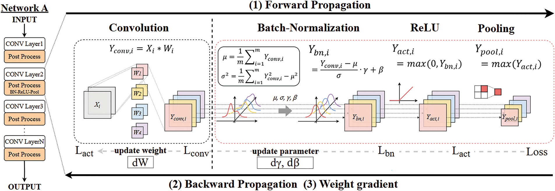
Figure 1: Layer configuration and computation diagram of CNN training

Training a CNN involves both forward and backward propagation, along with weight updates. During the forward pass, features propagate the network. The mini-batch feature is normalized by BN to maintain a distribution conducive to learning for each mini-batch. Backward propagation then computes gradients by propagating the cost function backward through the network. The sections below further explain the forward and backward processes of BN.

2.1 Forward Propagation

Batch normalization performs standardization and scaling of feature maps during training, ensuring consistent distribution across mini-batches. This process involves two steps: normalize and rescale. The normalization step subtracts the mean and divides by the variance for each channel. This can introduce a zero-mean, unit-variance distribution. Subsequently, the normalized distribution is then adjusted using the learnable parameters, gamma (γ) and beta (β). This rescales and shifts the data, allowing the network to adjust and optimize feature representation.

For a mini-batch of input feature, Xc∈RB×H×W, where c is the channel number, B is the mini-batch size, H is the feature map’s height and W is the width. BN is performed as Eqs. (1)–(4), where the xi means ith element of Xc, and m is total size of Xc. Eqs. (1) and (2) describe the statistical parameter, mini-batch’s mean and variance used for normalization step. Eq. (3) represents the normalization process, while Eq. (4) applies scaling and shifting to the normalized distribution using learnable parameters.

μ=1m∑i=1mxi,// mini-batch's mean(1)

σ2=1m∑i=1m(xi−μ)2,// mini-batch's variance(2)

xi^=xi−μσ2+ε,// normalize(3)

yi=γxi^+β,//scale and shift(4)

Inference and training follow distinct processes. In inference, the BN layer uses pre-trained parameters, such as the running mean and running variance. In Contrast, during training, the BN layer computes the mean and variance for every mini-batch and normalizes the input features accordingly. This mini-batch-based normalization introduces additional latency. Additionally, training requires excessive dynamic random-access memory (DRAM) access. This is because it needs to read the convolution layer’s output and write the BN layer’s normalized results (xi^) for backward propagation. Fig. 2 illustrates the differences of external memory access between inference and forward propagation during training. Here, the normalized value x^ is denoted as Xbn, and the output of normalization layer is referred to as Ybn.

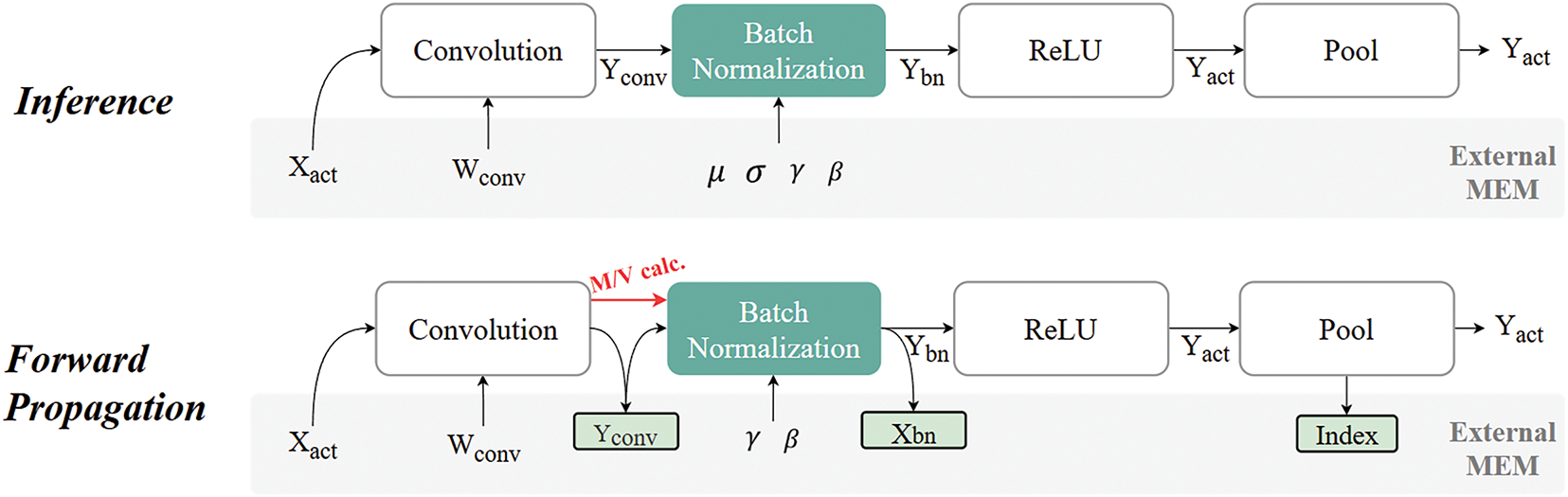
Figure 2: Difference of external memory access between inference and forward propagation during training

In inference, only a single image and weights of the convolution and batch normalization layers are loaded for each process. Unlike training, inference bypasses additional operations such as mean and variance calculations since it relies entirely on pre-computed data stored in external memory. On the other hand, training processes a mini-batch, typically consisting of 8 or 32 images, along with the required weights. During forward propagation, the normalization layer computes the mean and variance for mini-batch. This process necessitates storing all convolution results and reloading them from external memory to normalize the features.

2.2 Backward Propagation

Backward propagation involves complex operations due to the chain rule. Eqs. (5)–(7) represent the gradients of BN layer and its parameters, while Eq. (8) describes the parameter update formula based on SGD. Specifically, Eq. (5) provides the partial derivative of the BN layer, quantifying the change from the layer’s output to the input loss. The gradient of intermediate values, such as normalized values, mean and variance, influence this derivative, adding complexity to the backward process.

The gradient of gamma is calculated as the accumulated sum of the output loss gradient multiplied by x^, as described in Eq. (6). Similarly, the gradient of beta is calculated by summing the output loss gradient, as shown in Eq. (7). Finally, the computed parameter gradients are updated using the formula in Eq. (8). The variable P indicates the learnable parameter gamma and beta, and lr demonstrates learning rate.

∂L∂xi=∂L∂xi^⋅1σ2+ε+∂L∂σ2⋅2(xi−μ)m+∂L∂μ⋅1m,//gradient of BN layer(5)

∂L∂γ=∑i=1m∂L∂yixi^,//gradient of gamma(6)

∂L∂β=∑i=1m∂L∂yi,//gradient of beta(7)

P←P−lr⋅∂L∂P,//parameter update(8)

3  Proposed Optimization Methodology

3.1 Formula Rearrangement

To implement hardware-optimized normalization, it is necessary to reorganize the normalization formula. In the forward pass, variance can be calculated using random variable variance instead of sample variance. Sample variance, described in Eq. (2), requires reloading input samples after computing the mean, leading to additional external memory access. This inefficient computation increases power consumption and causes latency due to frequent interactions with external memory. To address these inefficiencies, the random variable variance in Eq. (9) is adopted. From a statistical perspective, each mini-batch in a deep neural network can be considered a set of samples drawn independently from the distribution of a random variable. The mean and variance of each mini-batch per channel converge to the population mean and variance, in accordance with the Central Limit Theorem. Using Eq. (9), the mean and variance can be computed simultaneously in parallel, where E[x] is the expectation of Xc.

σ2=V[Xc]=E[Xc2]−E[Xc]2.(9)

Particularly, backward propagation requires extensive computations, with additional complexity arising from the gradients of the mean, variance, and intermediate results, as shown in Eq. (5). To solve this, Eq. (5) is reorganized to better reflect the flow for hardware implementation. The gradients of each intermediate value are calculated using partial derivatives. First, we compute the gradient of the normalized value, then derive gradients for variance and mean, which are then substituted into the original formula to obtain a more hardware-friendly expression. Finally, the rearranged formula is presented in Eq. (10). This formula is derived by calculating the gradients of the intermediate values using the chain rule and substituting them accordingly. The square root of the variance added epsilon (ε) is approximated as the standard deviation (σ) for simplification. Using this approach, the gradient sequence input to the BN layer can be computed by subtracting the scaled normalization tensor, obtained during the forward pass, at the same positions.

∂L∂xi^=∂L∂yi⋅γ,//gradient of normalized xi^

∂L∂σ2=−12(σ2+ε)2∑j=1m∂L∂xj^⋅xj^,//gradient of variance

∂L∂μ=−1σ2+ε∑j=1m∂L∂xj^,//gradient of mean

∂L∂xi=∂L∂xi^⋅1σ2+ε+∂L∂σ2⋅2(xi−μ)m+∂L∂μ⋅1m,//original formula

=∂L∂yi⋅γσ2+ε+−12(σ2+ε)2∑j=1m∂L∂xj^xj^⋅2(xi−μ)m+−1σ2+ε∑j=1m∂L∂xj^⋅1m

=γσ[∂L∂yi−1m(xi^∑j=1m∂L∂yjxj^+∑j=1m∂L∂yj)],(∵σ2+ε≅σ)

=γσ⋅∂L∂yi−γσ⋅1m[(∂L∂γ⋅xi^+∂L∂β)],//rearranged formula(10)

3.2 Resource-Sharing

Batch normalization involves two stages in both forward and backward passes. In the forward pass, Stage 1 calculates mean and variance, while Stage 2 normalizes input features. In the backward pass, Stage 1 computes gamma and beta gradients, and Stage 2 derives the BN activation gradient. Parameter updates occur after all backpropagation steps.

However, mean/variance accumulation in forward Stage 1 overlaps with gradient accumulation in backward Stage 1. Implementing these operations separately would require at least two extra adders and one multiplier. To avoid this overhead, we propose block sharing. The hardware structure in Fig. 3 reuses the same computation flow at different time steps, reducing resource redundancy and improving efficiency.

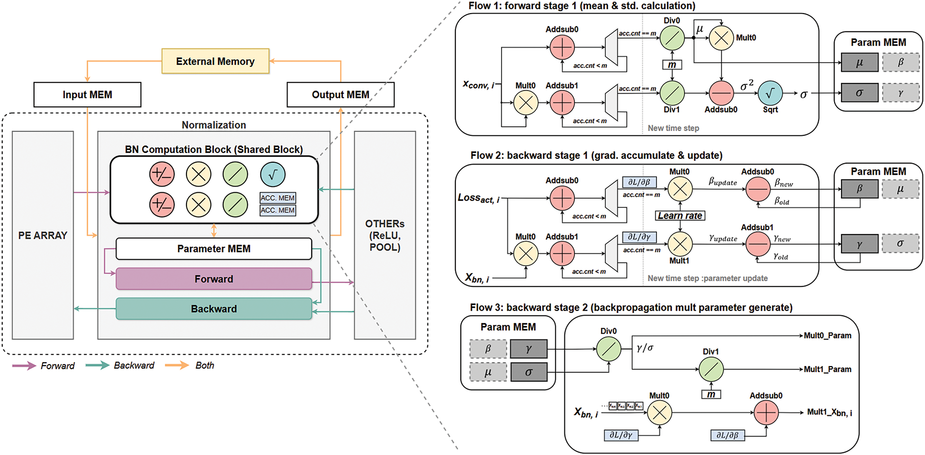
Figure 3: Overall architecture of proposed BN block and shared block’s flow

The normalization module consists of a computation block, parameter memory, and forward/backward blocks. The computation block includes seven shared units: two add/sub units, two multipliers, two dividers, one square root unit, and an accumulation buffer. These units handle the majority of the computational workload. Fig. 3 shows how it is used during Forward Stage 1, Backward Stage 1, and Backward Stage 2.

In the forward pass, outputs and squared outputs from the processing element (PE) array are accumulated per channel for each mini-batch. Once all mini-batch accumulations are complete, the system moves to a new time step and reuses the same functional units to compute both the mean and standard deviation. In the backward pass, loss gradients (after pooling and ReLU) are accumulated to compute gamma and beta gradients. These gradients are stored in a buffer and applied once Stage 2 finishes. Stage 2 then generates the inputs needed for the backward block.

The parameter memory stores the mean, variance, gamma, and beta values computed by the computation block. These parameters are updated during training. The forward block contains logic for Eqs. (3) and (4), and the backward block handles Eq. (10). Fig. 4a and b shows the overall computation flow, which includes the forward and backward blocks. The forward block can also be used for inference, and inputs to the backward block are concurrently computed in the shared computation block.

Figure 4: Computation flow of BN block: (a) forward; (b) backward

3.3 Interleaved Buffer

Most prior work using smaller datasets, such as modified national institute of standards and technology database (MNIST), kept all data in on-chip memory [30]. However, larger datasets (e.g., PASCAL Visual Object Classes (VOC) and ImageNet) require external DRAM to store parameters and outputs. To efficiently handle DRAM access for batch normalization (BN), we adopt a dual input buffer. Two first-in-first-out (FIFO) buffers store data in n-column chunks when n × n pooling is used. The purpose of processing a two-column image is to guarantee that four adjacent pixels are consistently available for 2 × 2 pooling. This approach enables parallel reading, normalizing, and writing operations without having to wait for an entire tile.

In single buffer design, the BN circuit would idle while data reads/writes for each tile, increasing delay. By contrast, our dual buffer approach shown in Fig. 5a divides the tile into two-column units, improving continuous input to the BN hardware and reducing internal storage from a full-tile buffer to a much smaller dual-column buffer. The buffer size reduction follows as Eqs. (11) and (12).

Singlebuffersize=Tile_width×Tile_height×Data_width(11)

Dualbuffersize=2×2×Tile_height×Data_width(12)

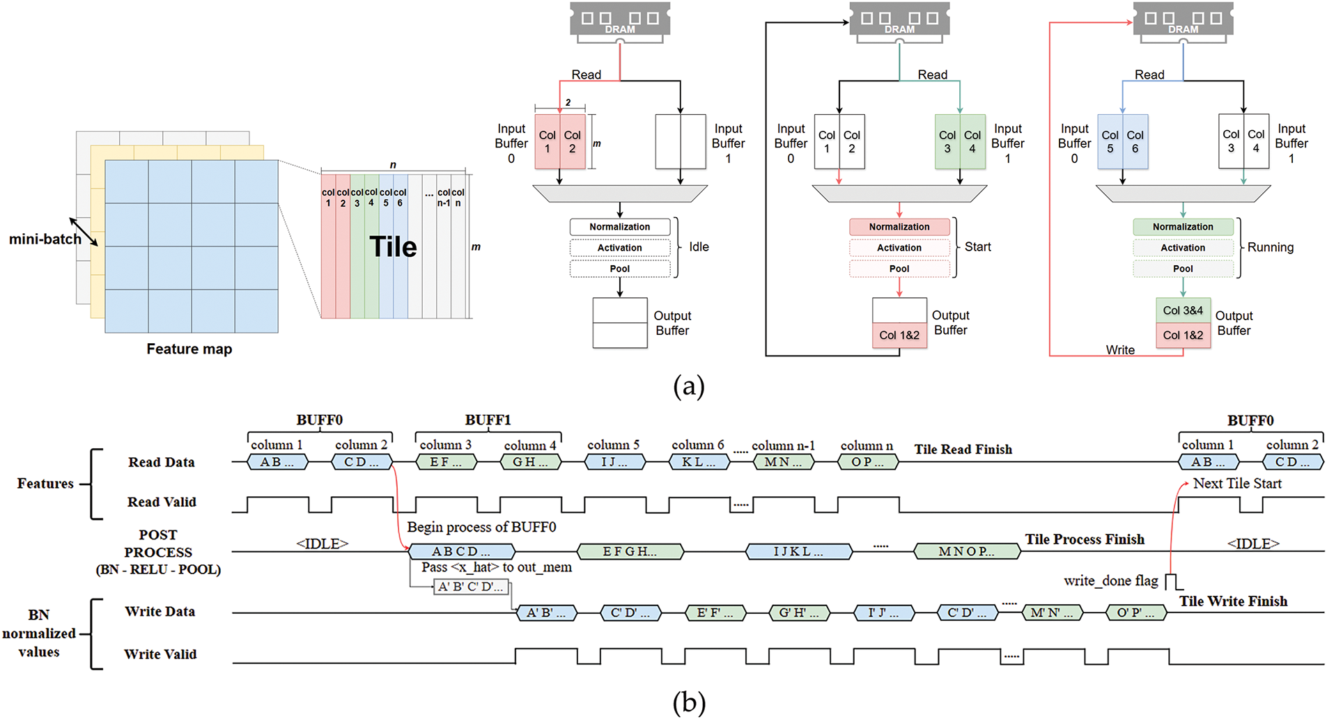
Figure 5: Interleaved buffer for normalization: (a) process architecture; (b) timing diagram

Here, “2 × 2” represents the dual buffers, each processing two columns. Therefore, this can reduce the buffer size to ‘4/tile_width’ compared to the single buffer. As tile width grows, the memory savings become more significant.

Fig. 5b illustrates the timing of read, post-process, and write with dual input buffer applied. It goes through the following steps:

1)   BUFF0 reads two columns from DRAM, while the post-processing circuit remains idle.

2)   BUFF1 begins filling with the next two columns as BUFF0 is processed.

3)   Completed BN results are written back to DRAM, then a write-done flag triggers the next read.

4)   This procedure repeats for all channels, ensuring the BN circuit does not idle for a full tile-read/write cycle.

The proposed pipeline (Eqs. (13) and (14)) achieves about a 53% speedup in post-processing compared to a single-buffer tile-based approach. By overlapping read, write, and BN operations in smaller units, we minimize DRAM access delays and resource requirements, making is especially advantageous for larger tile size.

Tileunitprocess=tread:1c×(Wt)+tprocess:1c×(Wt)+twrite:1c×(Wt)(13)

Columnunitprocess=tread:1c×(2)+tprocess:2c×(Wt2)+twrite:1c×(2)(14)

(Wt: Tile width)

(tread:1c: 1-column read time)

(tprocess:nc: n-column process time)

(twrite:1c: 1-column write time)

3.4 Zero-Skipping for Sparse Parameter Gradient

In batch normalization, gamma and beta gradients are obtained by adding up output gradients. When zero gradients exist, their accumulation has no effect on the final result. In particular, non-maximum entries result in zero gradients when using max pooling. These values can be skipped because they have no effect on the output.

Fig. 6a,b illustrates how zero-skipping applies to gamma and beta gradient calculations under max pooling. Without zero-skipping, in a 2 × 2 max pool, three of the four pixels are zero, making 3/4 of the gradient map redundant. By skipping non-maximum zero gradients, the computational load is effectively reduced to 1/4 of the original cost.

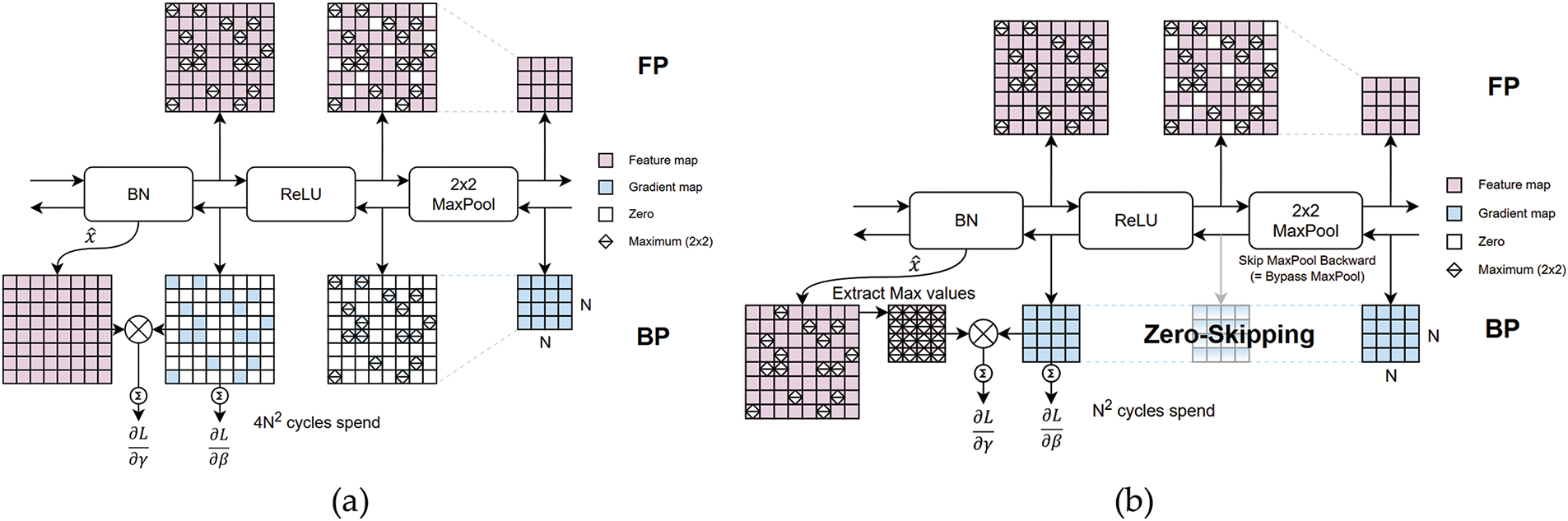
Figure 6: Data sparsity on maxpool layer: (a) without zero-skip; (b) with zero-skip

A prior study [28] also highlighted gradient sparsity in BN backward operations when ReLU layer produces zero gradients for negative inputs. Similarly, designing BN backward logic with awareness of upstream operations, such as max pooling can further optimize efficiency by leveraging data sparsity.

3.5 Square Root Design for High Accuracy

Ensuring high accuracy in standard deviation calculations requires avoiding approximations. However, square root operations introduce substantial hardware overhead. Many conventional approaches rely on iterative approximation methods—such as CORDIC [33,34] or Newton-Raphson [35]—that increase cycles and latency. Others use LUT-based Taylor expansions [36,37], incurring additional on-chip memory costs.

To address this, we apply the method from [38] to design a low-cost square root unit targeting bfloat16 precision. Cubic spline interpolation determines the mantissa, while integer operations and bit-shifting set the exponent. This approach eliminates the need for LUTs and iterative approximations, reducing hardware costs and making it suitable for the BN block.

4  Hardware Implementation and Verification

We implement the proposed, resource-efficient normalization accelerator in Vivado Verilog RTL. Its performance is compared to an Intel CPU and other works in terms of hardware size, resource usage, and power efficiency. To evaluate performance within a neural processing unit (NPU), we integrate the normalization block into the diagonal cyclic array structure from [39]. We target the You Only Look Once version 2 tiny (YOLOv2-tiny) CNN detection model on the VOC dataset for demonstration.

Because the BN block follows the convolutional layer, its performance depends on the PE array structure. Here, the PE array outputs 16 channels, so we utilize 16 BN blocks to process all channels in parallel.

4.1 Accuracy Verification

We train a YOLOv2-tiny on the VOC dataset using PyTorch and implemented the forward and backward steps of batch normalization through the torch.autograd.Function class. As a baseline, we use nn.BatchNorm2d in floating point 32 bits (FP32) with a batch size of 8 for 160 epochs. To compare with approximation-based methods, we incorporate the bfloat16 square root design from [38] into standard BN and also experiment with full bfloat16 precision training.

Fig. 7 shows that our method closely maintains the original accuracy. Using FP32, the mean Average Precision (mAP@0.5, mean Average Precision with IoU threshold of 0.5) drops by only 0.51% compared to the PyTorch baseline. With bfloat16 precision, the accuracy loss is 1.35%. In contrast, approximation methods like L1BN and RBN degrade mAP by 6.58% and 4.83%, respectively. Although approximations save hardware cost, they significantly reduce accuracy. Our standard BN approach keeps the accuracy high with minimal penalty. Hardware simulation results match the PyTorch model’s bfloat16 outcomes, confirming correctness.

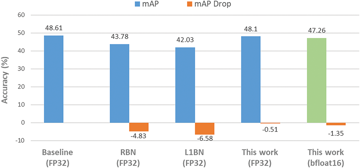
Figure 7: Training results comparison with other approximate approaches

4.2 BN Block

4.2.1 Experimental Setup

We conducted two main experiments. One uses a CPU for software execution and the other uses an FPGA board for hardware processing. Although we used YOLOv2-tiny (batch size = 8) to measure the forward and backward latency of the normalization block for validation, the proposed design is model-agnostic and can be applied to any architecture containing BN layers. Processing time was measured per layer, and the detailed specifications are as follows:

(1)   SW-CPU: We used an Intel Core i5-1135G7 processor (8 MB Cache, 2.4 GHz with 4 physical cores and 8 threads). The software implementation employed the PyTorch ‘nn.BatchNorm2d’ module. The CPU operated at maximum frequency with fully utilized threads to ensure a fair comparison.

(2)   HW-FPGA: Our design with 16 parallel BN blocks is implemented on Xilinx Virtex UltraScale+ VCU118 FPGA platform. The device has 1182 K+ LookUp Tables (LUTs), 2364 K+ Flip-Flops (FFs), 2160 × 36 KB Block RAMs (BRAMs), 6.8 K+ Digital Signal Processor (DSP) slices and 6 Peripheral Component Interconnect Express (PCIe). The Target frequency is set to 100 MHz.

4.2.2 Experimental Results and Analysis

Table 1 summarizes the results under these conditions. It includes the input data size and processing time (sum of forward and backward latency) for each normalization layer in YOLOv2-tiny. For clarity, decimal places are omitted to consider significant figures.

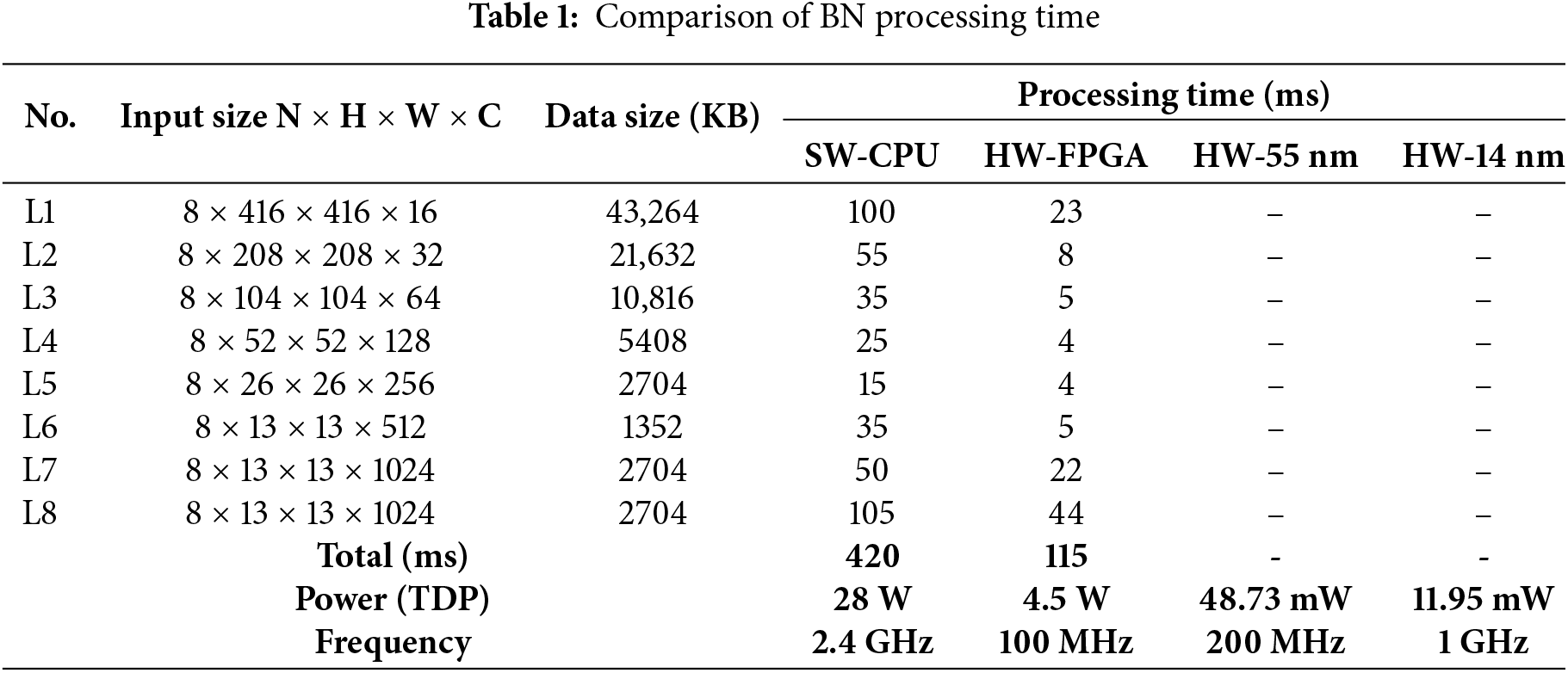
Under SW-CPU execution, the total runtime is 420 ms. In contrast, the HW-FPGA implementation takes only 115 ms, achieving a 72% speed improvement. Moreover, when compared to the CPU, the hardware implementation of the proposed normalization circuit exhibited 84% higher power efficiency.

Examining individual layers, layers with relatively fewer channels (1 to 4) show roughly a 5 times speed increase, while layers with more channels (7 and 8) show less improvement. This limitation arises from using 16 parallel BN blocks, which are less effective for larger numbers of channels. Nevertheless, the proposed hardware design still outperforms the CPU in both speed and power efficiency.

Finally, when synthesized in the TSMC 55 nm process at 200 MHz, the designed circuit consumed approximately 48.73 mW of power. When a process of the accelerator chip is estimated with a 14 nm Samsung process, it is predicted to operate at 1 GHz and consume about 11.95 mW. Table 1 compares the SW-CPU’s performance with the proposed accelerator implementation in FPGA (HW-FPGA), SoC in 55 nm Process (HW-55 nm), and SoC in 14 nm Process (HW-14 nm).

4.3 BN Block Comparison with Prior Works

We compare our design with prior works, including [26–28,30], summarized in Table 2. Overall, our approach delivers superior performance in terms of latency and power efficiency when compared to both approximate and standard BN implementations. As we have discussed, it is important to note that the number of parallel BN blocks used in each design varies according to the output channels of the PE array. Therefore, to facilitate a fair resource comparison, we normalized each design’s reported resource usage by dividing it by the number of BN blocks they employed. Moreover, the synthesized chip area also has different processes. Consequently, we define the unit cell and write the approximate number of cells.

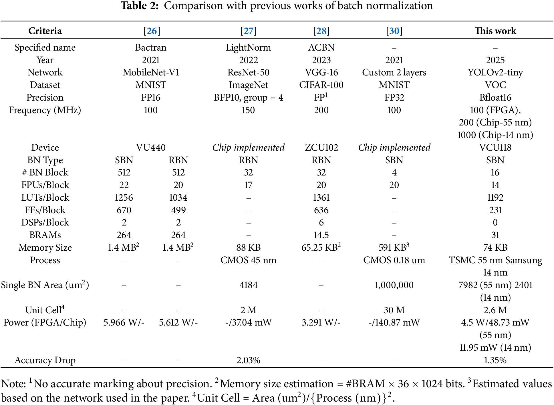
Bactran [26] integrates BN within each of its 512 PEs, introducing a standard BN (SBN) but at higher hardware cost than our method. They also propose an approximate range BN (RBN), which still consumes more power and overall resources (except for LUTs) than our design. LightNorm [27] applies RBN and lower precision to reduce the area, but has an accuracy trade-off. ACBN [28] also adopts RBN and leverages data sparsity, yet our shared-block structure uses fewer computing units while retaining SBN. In [30], SBN without external memory required large on-chip storage. In contrast, our method uses fewer resources and still applies standard BN efficiently. Overall, our approach provides a low-cost standard BN accelerator, outperforming approximation-based designs in resource efficiency and power consumption.

4.4 NPU with BN Block

We integrate the BN block into the NPU design from [39], which uses a diagonal cyclic array with 2304 multiply-accumulate (MAC) units. To verify the design, we implement it on an FPGA based on Virtex UltraScale+ VU19P with 4085 K+ LUTs, 8171 K+ FFs, 2160 × 36 KB BRAMs, 3.8 K+ DSP slices and 8 PCIe. This performs training operation for CNN model called YOLOv2-tiny using the VOC datasets.

Table 3 shows the comparison result of training performance. Compared to an AMD Ryzen 5 5600X CPU and an embedded RISC-V core (both operating with the same hardware environment), our integrated BN block at 100 MHz improved performance by 63% over the CPU and by 97% over RISC-V. The CPU spent about one second on data caching, and the RISC-V was even slower due to limited optimization. Both of them also include interrupt handling time. By contrast, our BN accelerator avoided these delays.

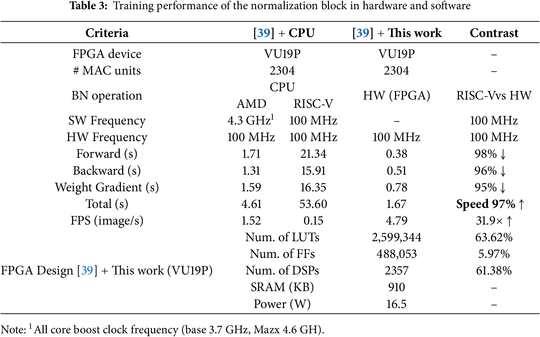
For clarification, the ‘ [39] +CPU’ configuration in Table 3 represents the total processing time including interrupt handling when the existing NPU design (without a normalization accelerator) relies on the CPU to handle normalization’s forward and backward operations. Meanwhile, the ‘ [39] +this work’ configuration shows the results when our proposed BN training IP is integrated into the NPU instead of using the CPU for normalization tasks. This demonstrates that our hardware BN design enhances overall NPU training performance.

5  Conclusion

Batch normalization (BN) plays a critical role in training convolutional neural networks; however, its large computational requirements make hardware implementation complex and challenging. Particularly, the standard deviation calculation increases hardware overhead due to the sum of squares and square root operations. In this work, we propose an efficient standard BN hardware design that significantly reduces overhead. By sharing hardware resources for forward and backward propagation, we reduce floating-point units by 36% compared to SBN and by 30% relative to [30]. Additionally, our dual-input buffering minimizes on-chip memory requirements, and zero-skipping in the backward pass lowers computations by a factor of 1/n2 in the n × n max-pooling layer.

Our implementation on a VCU118 FPGA achieves 72% speedup and 83% higher power efficiency than an Intel CPU. Integrated into the existing NPU, our BN accelerator at 100 MHz also demonstrates 63% and 97% faster performance compared to a 4.3 GHz AMD CPU and an embedded RISC-V at 100 MHz, respectively. These results underscore the effectiveness of the proposed BN accelerator, suggesting that it can be a compelling solution for various hardware-accelerated AI applications moving forward.

Despite these advantages, our approach has certain limitations. First, the square root unit used for standard deviation calculation is optimized for a specific precision target (bfloat16). If implementations with different precision requirements are needed, additional dedicated computation units would be required. Second, our design optimizes on-chip memory and forward/backward propagation flow specifically for bat normalization. Since it’s tailored for BN, applying it to other normalization techniques such as LN or GN would require additional controllers for different datapaths.

Future efforts could explore hybrid precision approaches to accommodate varying model requirements, as well as dynamic scheduling or approximate computation strategies tailored for edge devices. Investigating advanced memory hierarchies or dataflow optimizations may further improve performance and efficiency, expanding the applicability of this BN accelerator in next-generation AI systems.

Acknowledgement: The authors would also like to thank the respected editor and reviewer for their support.

Funding Statement: This work was supported by the National Research Foundation of Korea (NRF) grant for RLRC funded by the Korea government (MSIT) (No. 2022R1A5A8026986, RLRC) and was also supported by Institute of Information & Communications Technology Planning & Evaluation (IITP) grant funded by the Korea government (MSIT) (No. 2020-0-01304, Development of Self-Learnable Mobile Recursive Neural Network Processor Technology). It was supported by the MSIT (Ministry of Science and ICT), Republic of Korea, under the Grand Information Technology Research Center support program (IITP-2024-2020-0-01462, Grand-ICT) supervised by the IITP (Institute for Information & Communications Technology Planning & Evaluation) and it was supported by the Korea Technology and Information Promotion Agency for SMEs (TIPA) and supported by the Korean government (Ministry of SMEs and Startups)’s Smart Manufacturing Innovation R&D (RS-2024-00434259).

Author Contributions: As the primary, Go-Eun Woo is the main contributor in the detailed theory, implementation, and evaluating the performance of the presented research. Sang-Bo Park made contributions in defining the architecture and improving the performance of the NPU design. Gi-Tae Park made contributions in verifying the NPU design in FPGA. Muhammad Junaid made contributions in developing accurate simulator for training operation with brain-16 floating point format based on CUDA programming. As the advisor, Hyung-Won Kim guided the research direction and reviewed NPU design and performance evaluation. All authors reviewed the results and approved the final version of the manuscript.

Availability of Data and Materials: Not applicable.

Ethics Approval: Not applicable.

Conflicts of Interest: The authors declare no conflicts of interest to report regarding the present study.

References

1. LeCun Y, Bengio Y, Hinton GE. Deep learning. Nature. 2015;521(7553):436–44. doi:10.1038/nature14539. [Google Scholar] [PubMed] [CrossRef]

2. Hochreiter S. The vanishing gradient problem during learning recurrent neural nets and problem solutions. Int J Uncertain Fuzz Knowl Based Syst. 1998;6(2):107–16. doi:10.1142/S0218488598000094. [Google Scholar] [CrossRef]

3. Hanin B. Which neural net architectures give rise to exploding and vanishing gradients? Vol. 31. In: Advances in neural information processing systems. Montreal, Canada. Red Hook, NY, USA: Curran Associates, Inc.; 2018. [Google Scholar]

4. Ying X. An overview of overfitting and its solutions. J Phy Conf Series. 2019;1168(2):022022. doi:10.1088/1742-6596/1168/2/022022. [Google Scholar] [CrossRef]

5. Nair V, Hinton GE. Rectified linear units improve restricted Boltzmann machines. In: Proceedings of the 27th International Conference on Machine Learning (ICML-10); 2010 Jun 21–24; Haifa, Israel. p. 807–14. [Google Scholar]

6. Zhang J, He T, Sra S, Jadbabaie A. Why gradient clipping accelerates training: a theoretical justification for adaptivity. In: International Conference on Learning Representations ICLR 2020; 2020 Apr 30; Addis Ababa, Ethiopia. doi:10.48550/arXiv.1905.11881. [Google Scholar] [CrossRef]

7. Nitish S, Hinton GE, Krizhevesky A, Sutskever I, Salakhutdinov R. Dropout: a simple way to prevent neural networks from overfitting. J Mach Learn Res. 2014;15(1):1929–58. [Google Scholar]

8. Ioffe S, Szegedy C. Batch normalization: accelerating deep network training by reducing internal covariate shift. arXiv:1502.03167. 2015. [Google Scholar]

9. Krizhevsky A, Sutskever I, Hinton GE. Imagenet classification with deep convolutional neural networks. Vol. 25. In: Advances in neural information processing systems. Lake Tahoe, NV, USA. Red Hook, NY, USA: Curran Associates, Inc.; 2012. [Google Scholar]

10. Santurkar S, Tsipras D, Ilyas A, Madry A. How does batch normalization help optimization? Vol. 31. In: Advances in neural information processing systems. Montreal, Canada. Red Hook, NY, USA: Curran Associates, Inc.; 2018. [Google Scholar]

11. Li Y, Wang N, Shi J, Liu J, Hou X. Revisiting batch normalization for practical domain adaptation. arXiv:1603.04779. 2016. [Google Scholar]

12. Summers C, Dinneen MJ. Four things everyone should know to improve batch normalization. arXiv:1906.03548. 2019. [Google Scholar]

13. Bjorck N, Gomes CP, Selman B, Weinberger KQ. Understanding batch normalization. Vol. 31. In: Advances in neural information processing systems. Montreal, Canada. Red Hook, NY, USA: Curran Associates, Inc.; 2018. [Google Scholar]

14. Sun J, Cao X, Liang H, Huang W, Chen Z, Li Z. New interpretations of normalization methods in deep learning. Proc AAAI Conf Artif Intell. 2020;34(4):5875–82. doi:10.1609/aaai.v34i04.6046. [Google Scholar] [CrossRef]

15. Ioffe S. Batch renormalization: towards reducing minibatch dependence in batch-normalized models. Vol. 30. In: Advances in neural information processing systems. Long Beach, CA, USA. Red Hook, NY, USA: Curran Associates, Inc.; 2017. [Google Scholar]

16. Garbin C, Zhu X, Marques O. Dropout vs. batch normalization: an empirical study of their impact to deep learning. Multimed Tools Appl. 2020;79(19):12777–12815. doi:10.1007/s11042-019-08453-9. [Google Scholar] [CrossRef]

17. Thakkar V, Tewary S, Chakraborty C. Batch normalization in convolutional neural networks—a comparative study with CIFAR-10 data. In: 2018 Fifth International Conference on Emerging Applications of Information Technology (EAIT); 2018 Jan 12–13; Kolkata, India. p. 1–5. doi:10.1109/EAIT.2018.8470438. [Google Scholar] [CrossRef]

18. Lubana ES, Dick R, Tanaka H. Beyond batchnorm: towards a unified understanding of normalization in deep learning. Adv Neural Inf Process Syst. 2021;34:4778–91. [Google Scholar]

19. Junaid M, Aliev H, Park S, Kim H, Yoo H, Sim S. Hybrid Precision Floating-Point (HPFP) selection to optimize hardware-constrained accelerator for CNN training. Sensors. 2024;24(7):2145. doi:10.3390/s24072145. [Google Scholar] [PubMed] [CrossRef]

20. Ba JL, Kiros JR, Hinton GE. Layer normalization. arXiv:1607.06450. 2016. [Google Scholar]

21. Huang X, Belongie S. Arbitrary style transfer in real-time with adaptive instance normalization. In: Proceedings of the 2017 IEEE International Conference on Computer Vision (ICCV); 2017 Oct 22–29; Venice, Italy. p. 1501–10. [Google Scholar]

22. Wu Y, He K. Group normalization. In: Proceedings of the 2018 European Conference on Computer Vision (ECCV); 2018 Sep 8–14; Munich, Germany. p. 3–19. [Google Scholar]

23. Rumelhart DE, Hinton GE, Williams RJ. Learning representations by back-propagating errors. Nature. 1986;323(6088):533–6. doi:10.1038/323533a0. [Google Scholar] [CrossRef]

24. Banner R, Hubara I, Hoffer E, Soudry D. Scalable methods for 8-bit training of neural networks. Vol. 31, In: Advances in neural information processing systems. Montreal, QC, Canada. Red Hook, NY, USA: Curran Associates, Inc.; 2018. [Google Scholar]

25. Soudry D, Hubara I, Meir R. Expectation backpropagation: parameter-free training of multilayer neural networks with continuous or discrete weights. Vol. 27. In: Advances in neural information processing systems. Montreal, QC, Canada. Red Hook, NY, USA: Curran Associates, Inc.; 2014. [Google Scholar]

26. Yang Z, Wang L, Luo L, Li S, Guo S, Wang S. Bactran: a hardware batch normalization implementation for CNN training engine. IEEE Embedd Syst Lett. 2021;13(1):29–32. doi:10.1109/LES.2020.2975055. [Google Scholar] [CrossRef]

27. Noh SH, Park J, Park D, Koo J, Choi J, Kung J. LightNorm: Area and Energy-Efficient Batch Normalization Hardware for On-Device DNN Training. In: 2022 IEEE 40th International Conference on Computer Design (ICCD); 2022 Oct 23–26; Olympic Valley, CA, USA; 2022. p. 443–50. doi:10.1109/ICCD56317.2022.00072. [Google Scholar] [CrossRef]

28. Li B, Wang H, Luo F, Zhang X, Sun H, Zheng N. ACBN: approximate calculated batch normalization for efficient DNN on-device training processor. IEEE Trans Very Large Scale Integr (VLSI) Syst. 2023;31(6):738–48. doi:10.1109/TVLSI.2023.3262787. [Google Scholar] [CrossRef]

29. Wu S, Li G, Deng L, Liu L, Wu D, Xie Y, et al. L1-Norm batch normalization for efficient training of deep neural networks. IEEE Trans Neural Netw Learn Syst. Jul 2019;30(7):2043–51. doi:10.1109/TNNLS.2018.2876179. [Google Scholar] [PubMed] [CrossRef]

30. Ting YS, Teng YF, Chiueh TD. Batch normalization processor design for convolution neural network training and inference. In: 2021 IEEE International Symposium on Circuits and Systems (ISCAS); 2021 May 22–28; Daegu, Republic of Korea. p. 1–4. doi:10.1109/ISCAS51556.2021.9401434. [Google Scholar] [CrossRef]

31. Ge J, Cui X, Xiao K, Zou C, Chen Y, Wei R, et al. BNReLU: combine batch normalization and rectified linear unit to reduce hardware overhead. In: 2019 IEEE 13th International Conference on ASIC (ASICON); 2019 Oct 29–Nov 1; Chongqing, China; 2019. p. 1–4. doi:10.1109/ASICON47005.2019.8983577. [Google Scholar] [CrossRef]

32. Singh S, Krishnan S. Filter response normalization layer: Eliminating batch dependence in the training of deep neural networks. In: Proceedings of the IEEE/CVF Conference on Computer Vision and Pattern Recognition; 2020 Jun 13–19; Seattle, WA, USA; 2020. p. 11237–46. [Google Scholar]

33. Hong W, Chen H, Quan L, Fu Y, Li L. Low-cost high-precision architecture for arbitrary floating-point nth root computation. In: 2023 IEEE International Symposium on Circuits and Systems (ISCAS); 2023 May 21–25; Monterey, CA, USA; 2023. p. 1–5. doi:10.1109/ISCAS46773.2023.10181944. [Google Scholar] [CrossRef]

34. Ray A. A survey of CORDIC algorithms for FPGA based computers. In: Proceedings of the 1998 ACM/SIGDA Sixth International Symposium on Field Programmable Gate Arrays; 1998 Feb 22–25; Monterey, CA, USA. p. 191–200. [Google Scholar]

35. Wang LK, Schulte MJ. Decimal floating-point square root using Newton-Raphson iteration. In: 2005 IEEE International Conference on Application-Specific Systems, Architecture Processors (ASAP’05); 2005 Jul 23–25; Samos, Greece. p. 309–15. doi:10.1109/ASAP.2005.29. [Google Scholar] [CrossRef]

36. Wei J, Kuwana A, Kobayashi H, Kubo K, Tanaka Y. Floating-point square root calculation algorithm based on taylor-series expansion and region division. In: 2021 IEEE International Midwest Symposium on Circuits and Systems (MWSCAS); 2021 Aug 9–11; Lansing, MI, USA. p. 774–8. [Google Scholar]

37. Kwon TJ, Draper J. Floating-point division and square root implementation using a taylor-series expansion algorithm with reduced look-up tables. In: 51st Midwest Symposium on Circuits and Systems; 2008 Aug 10–13; Knoxville, TN, USA. p. 954–7. doi:10.1109/MWSCAS.2008.4616959. [Google Scholar] [CrossRef]

38. Woo GE, Kim HW. Cubic spline interpolation square-root compute unit for cost-efficient batch-normalization calculation of accurate DNN training. J Inst Electron Inf Eng. 2025;62(2):19–28. (In Korean). [Google Scholar]

39. Park SB. Reconfigurable CNN Training Accelerator Design Based on Efficient Memory Access Reduction Techniques [master’s thesis]. Cheongju, Republic of Korea: Chungbuk National University; 2024. [Google Scholar]