Graph-Embedded Neural Architecture Search: A Variational Approach for Optimized Model Design

1  Introduction

In recent years, neural architecture search (NAS), which automatically explores optimal neural network architectures customized based on the characteristics of datasets and tasks, has played a crucial role in AutoML. Network architectures have conventionally been designed through trial-and-error handcrafting, an approach that necessitates specialized expertise and substantial time to improve performance.

However, NAS faces the challenge of long computational times required for architecture searches. Conducting a full architectural search each time a new dataset emerges is highly inefficient. To effectively address the increasingly diverse datasets expected in the future, techniques that can directly predict the optimal architecture of unseen datasets are required. If the optimal architecture could be directly predicted, it would substantially expedite the architecture generation process and would produce a marked reduction in the search time.

Various generation methods have been proposed, such as iterative random architecture generation or partial modifications of existing architectures. However, these approaches are constrained by limitations such as the inability to consider multiple candidates simultaneously and the difficulty in discovering high-quality solutions owing to their inherently discrete operations. This study focuses on methods that map architectures into a continuous latent feature space to address these issues. Specifically, we attempted to embed existing high-performance architectures in latent feature spaces, and subsequently estimate and generate architectures suitable for new datasets based on their local neighborhood information. We propose a framework called NAVIGATOR (Neural Architecture search using VarIational Graph AuTO-encodeR), which generates architectures appropriate for unseen datasets by mapping architectures that perform well on existing datasets into a latent feature space.

We employed an encoder-decoder transformation model for latent feature mapping based on variational graph auto-encoders (VGAE) [1]. VGAE excels at extracting features from graph structures using its encoder and decoder, rendering it particularly suitable for mapping NAS architectures. By minimizing the error between the input architecture and its reconstructed output, the latent representations are trained to capture the essential characteristics of each architecture. By training a VGAE on existing high-quality architectures, NAVIGATOR constructs a latent space and designs optimal architectures for diverse datasets. Furthermore, to define the similarity, we propose constructing the latent space by incorporating dataset features and task features. We demonstrated that the proposed method can generate architectures with a performance comparable to the performances of existing NAS methods, yet with significantly less search time. Architectural performance in the vicinity of the optimal solution was investigated. Considering architecture generation through the latent space as a form of information transfer, the distribution of architectures within this space significantly influences the performance of the method. An overview of the NAVIGATOR is presented in Fig. 1.

Figure 1: Schematic of the proposed approach

The preliminary version [2] of this study was presented at the 33rd International Conference on Artificial Neural Networks. The main updates since the previous version include additional experiments evaluating the utility of the proposed method and an extension of the framework to incorporate the dataset and task features. Each encoder of NAVIGATOR and the base method of the compositions of the contents were also verified as a new preliminary experiment. Furthermore, new validations were conducted to confirm the effectiveness of the proposed method.

2  Related Work

This section reviews related research on NAS methods and Graph Neural Network (GNN) relevant to this study.

2.1 Neural Architecture Search (NAS)

NAS is a subfield of AutoML dedicated to the automated search for optimal neural network 61 architectures in deep learning. NAS approaches primarily optimize two aspects: the connection patterns among the layers and the selection of operations to search for the optimal architecture. Early NAS methods based on evolutionary algorithms and reinforcement learning [3–6] were proposed; however, they required extremely high computational cost and time, prompting the need for a more efficient approach. Given the high computational cost of NAS-based architecture searches, efficient architectural representations were sought, leading to the emergence of cell-based NAS methods designed to reduce the search space. Among the cell-based NAS methods, DARTS [7] and PC-DARTS [8], which enable an efficient architecture search, have been established as representative methods. In these methods, an entire network is defined as a collection of compact modules (cells), with each cell represented as a directed acyclic graph (DAG), thereby enabling the construction of large-scale architecture within a confined search space. Recently, numerous high-accuracy architectures have been discovered using cell-based NAS algorithms [9], and the reuse of the high-performance architectures obtained via NAS is anticipated to be an important topic for future reuse. In addition to cell-based NAS methods, recent advancements have introduced innovative approaches that enhance both search efficiency and architecture performance. For instance, approaches that integrate NAS with self-adaptive techniques and evolutionary algorithms [10] effectively address challenges such as early convergence, bias, and inefficiency in operation selection. These methods contribute to a more robust and flexible architecture search. In addition, techniques that progressively activate partial channel connections across multiple stages have been proposed to balance computational costs and model accuracy. Specialized NAS approaches have also been developed for generative adversarial networks (GANs). Transformer-based NAS methods [11,12] have also demonstrated significant advancements in the structural representation refinement, which were difficult to achieve using earlier techniques. Moreover, incorporating large language models into the NAS framework has shown potential in improving architecture prediction and search guidance [13,14]. Collectively, these developments represent the leading edge of NAS research and highlight promising directions for future studies and practical applications.

2.2 Differentiable Architecture Search (DARTS)

DARTS is a cell-based NAS method that employs weight sharing and a gradient method to change the continuous search space, thereby enabling an efficient search of architectures. Weight sharing is a one-shot technique that selects architectural candidates in part of the supernet (a model that includes all network architecture candidates in the search space) of a directed acyclic graph. Eq. (1) pertains to two nodes in DARTS.

x(j)=∑i<jo(i,j)x(i)(1)

Eq. (2) is used for the search operation.

o¯(i,j)(x(i))=∑o∈Oexp⁡(αo(i,j))∑o′∈Oexp⁡(αo′(i,j))o(x(i))(2)

Herein, O is a candidate operation entering an edge, and the architecture weight of a pair of nodes (i,j) is a parameter α(i,j) of dimension |O|. The architecture weights α represent the significance of each candidate operation in determining the network architecture. When the search is completed, the architecture is determined using Eq. (3):

o(i,j)=argmaxo∈O⁡αo(i,j)(3)

DARTS searches for two types of cells: normal and reduced cells. When the search is completed, the architecture is generated by connecting two types of multiple cells.

2.3 Patrial Channel Connections for Memory-Efficient Architecture Search (PC-DARTS)

PC-DARTS, an enhanced version of DARTS, is a gradient-based method that can reduce the memory and computational time required to search network architectures. DARTS requires considerable memory because its target range is wide and includes a redundant search space. Contrarily, PC-DARTS combines edge normalization techniques, which can select a stable connection of the network, and a partial channel connection (Eq. (4)), which passes only part of the channel in the search operation for an efficient search.

S(i,j) is a masking function that assigns 1 to a selected channel and 0 to a masked channel.

oPC(i,j)(xi;S(i,j))=∑o∈Oexp⁡(αo(i,j))∑o′∈Oexp⁡(αo′(i,j))o(S(i,j)xi)+(1−S(i,j))xi(4)

PC-DARTS achieves performance gains of less than 0.1 GPU days, surpassing DARTS’s requirement of 1.0 GPU days. Moreover, the enhanced stability allows PC-DARTS to directly search neural architecture large datasets.

2.4 Graph Neural Network (GNN)

A GNN [15] is a deep learning model designed for graph-structured data and has been applied to tasks such as graph classification, edge prediction, and node classification. Because GNNs effectively process any data represented as nodes and edges, they have been applied across various fields including molecular structure analysis in chemistry [16,17] and multibody particle simulations in physics [18,19]. In this study, given that the generated NAS is represented in graph form, GNN methods were employed to process the graph-structured data as inputs. Many GNNs employ a convolution operation known as graph convolution network (GCN). In particular, GCN demonstrates high performance by extracting local graph information using the adjacency matrix and degree matrix, as shown in Eq. (5).

FN(l+1)=h(D−1/2AD−1/2FN(l)W(l))(5)

Here, FN represents the node features at the input and output of a layer. A is the matrix obtained by adding the identity matrix to the adjacency matrix (which indicates how edges connect in an undirected graph), W is a learnable weight matrix, D is the degree matrix representing node relationships, and h is an activation function (e.g., ReLU or Softmax). Additionally, the graph attention network (GAT) [20] has attracted significant attention as a method that enhances representational power by incorporating an attention mechanism into the GCN to consider the importance between nodes. Additional GNN layers have also been introduced, such as GraphSAGE [21], Chebyshev Networks [22], and Graph Isomorphism Network (GIN) [23].

Variational graph auto-encoders (VGAE) [24] are models that learn latent representations of graphs using an encoder-decoder framework and serve as core methods in this study. It extends the VAE [25] originally developed for images to enable the representation of graphs. The details of the encoder and decoder are provided in the following section.

The flexible structural representation capability of GNNs enables them to effectively encode complex problem structures, making them well-suited for a diverse array of optimization problems. Notable applications include methods to combinatorial optimization [26] and reinforcement learning approaches incorporating GNN as the agent’s state representation [27]. These studies demonstrate the utility of GNNs in solving various optimization tasks and are closely aligned with the objectives and methodology of the proposed research.

2.5 Related Approaches

Several approaches similar to the proposed method exist in the literature. The proposed method is characterized by the following five features:

(a)   Alleviating computational cost and search time is reduced

(b)   Building latent feature space using VGAE

(c)   Capable of handling continuous architecture

(d)   Directly generated architectures

(e)   Enabling information transfer in existing datasets

Owing to the substantial time and computational resources required for search, conventional NAS methods face significant challenges, prompting numerous studies aimed at substantially reducing the computational cost (a) [28–30]. Furthermore, numerous methods have been proposed to map features extracted from NAS to a latent space [31–34]. Among these, only a limited number–such as those in [35–37], employ VGAE to extract features, which distinguishes our approach in terms of (b). By employing VGAE, detailed features and properties of the architectures can be effectively captured through graph representations. Other related approaches include methods that construct a predictor to estimate performance [38–41] (graph-based approach [42–44]); however, our study adopts an approach (d) that directly generates architectures from the latent feature space. Moreover, by simultaneously learning the embedded representations of the operations, the proposed method can accommodate both discrete and continuous architectures (c). In terms of leveraging promising prior knowledge to enhance performance (e), the concept is akin to that of transfer learning [45–47]. While transfer learning methods primarily focus on transferring dataset information, the proposed method specializes in transferring the information of architectures themselves. Contrary to many related approaches that primarily aim to improve the accuracy, this study focuses on investigating architectural structures across various datasets. There were approaches with only a distinctive feature and those exhibiting multiple features. However, the proposed method possesses all five features, (a)–(e), making it significantly different from related research. All five features are critical for the generation of the architecture. The combination of these features provides multifaceted advantages and is expected to be applicable in a wide range of applications. Furthermore, a notable aspect of this study is that by using an improved VGAE, the detailed characteristics of the architectures explored through the NAS can be effectively captured. Another distinguishing feature of this study is the construction of architectures that can achieve high accuracies across multiple datasets.

In contrast to neural architecture optimization [48] and their subsequent Graph VAE-based extensions [49], NAVIGATOR adopts a substantially different framework from the perspective of design paradigm. These earlier methods primarily focus on optimizing performance within a single dataset, embedding only the architecture into the latent space. As a result, they often fail to account for the tasks or dataset diversity. By contrast, NAVIGATOR is explicitly designed to maximize transferability across various tasks and datasets. Concretely, it achieves this by separately encoding architectural structure and unstructured task information, which are then integrated in the latent space. This design enables NAVIGATOR to directly generate architectures tailored for previously unseen tasks, thereby demonstrating high flexibility and extensibility. Furthermore, NAVIGATOR’s configuration, which clearly separates the roles of each module, such as architecture encoder, dataset encoder, task encoder, and decoder, makes it particularly well-suited for future improvements and domain-specific applications.

3  Proposed Approach NAVIGATOR

This study proposes a Neural Architecture search using the NAVIGATOR. This method leverages the latent features obtained by integrating NAS and VGAE, thereby enabling the visualization of the discovered architectural characteristics and the generation of new architectures.

3.1 Overview of NAVIGATOR

Fig. 1 shows a schematic overview of the proposed method, and the details of the encoder and decoder are shown in Fig. 2. NAVIGATOR consists of three components: NAS, VGAE, and the generating model. The procedures described in Algorithm 1 (NAS: Lines 1–5, VGAE: Lines 6–15, Generating Model: Lines 16–19), the process proceeds accordingly. Initially, NAS was applied to a given dataset to obtain an optimized architecture. The number of obtained architectures depends on the type of dataset, and multiple searches were performed with different seeds. Subsequently, the encoder and decoder of VGAE were employed on the optimized architectures to extract latent features. As shown in Fig. 1, clustering can be performed using visualization techniques to generate new architectures after extracting the latent features. For visualization, we used PCA [50], a dimensionality reduction algorithm. Preliminary experiments tested other dimensionality reduction methods, PCA was adopted in this study because its mechanism aligns well with VGAE and it yielded more visually interpretable results.

Figure 2: Details of encoder & decoder. GAT: graph attention network; GCN: graph convolution network; edge classifier: two fully connected layers with a ReLU

3.2 Encoder

Let μ be the mean of the latent variables, and let σ be their variance. As shown in Eq. (6), the encoder computes μ and log⁡σ from the graph representing the network architecture discovered by NAS (node features FN, adjacency matrix A, and edge features FE).

μ=GNNμ(FN,A,FE)log⁡σ=GNNσ(FN,A,FE)(6)

Here, FN contains the node features, A is the adjacency matrix for the edges, and FE contains edge features. The node features FN consist of input, intermediate, and output nodes in the NAS, with these three types of nodes serving as the input features. For example, when combining the two cell types in PC-DARTS, there were four input nodes, eight intermediate nodes (hyperparameters), and two output nodes. In addition, the edge features FE of the graph were learned as input. The edge features FE depend on the NAS search space. In PC-DARTS, for instance, |O|=8 operation candidates were used (skip connection, none, average pooling 3 × 3, max pooling 3 × 3, separable convolution 3 × 3, separable convolution 5 × 5, dilated convolution 3 × 3, and dilated convolution 5 × 5). Each operator corresponds to an edge feature in FE that passes through an embedding layer. The embedding layer was also updated during training. By embedding edge features FE through this embedding layer, inter-edge relationships can be more effectively reflected in the latent space. Consequently, it becomes possible to capture not only the graph structure but also the edge information more comprehensively.

In the proposed method, the original VGAE is enhanced by adopting two types of layers: one that uses only GCN layers and another that combines GAT and GCN layers, as shown in Fig. 2. In the NAS search space considered in this study, each architecture typically includes multiple inputs and intricate skip connections. With its ability to assign varying importance to connections on a per-node basis through an attention mechanism, the GAT dynamically captures structural heterogeneity. This property effectively extracts architectural features that a GCN constrained by its fixed receptive field may not fully capture, thereby contributing to enhanced representational power. However, owing to the computation of weights for each edge, the model experiences significant computational cost and increased complexity. To balance this trade-off, we employ a stepwise configuration that integrates GAT and GCN layers. Concretely, the initial GAT layer is used to learn non-local and non-uniform relationships, while the subsequent GCN layer efficiently aggregates local graph structure information within the graph. This hybrid design balances representational expressiveness and computational efficiency. Moreover, such a design enables gradual control over model complexity and facilitates the learning of latent representations that can flexibly accommodate the diverse architecture within the search space.

The encoder in the proposed method captures topological properties through the VGAE framework, which learns the latent space by directly considering connection relationships among nodes. Specifically, the initial GAT layer extracts structural importance through attention mechanisms, while the subsequent GCN layer aggregates these features across nodes. This process enables the emergence of structural characteristics as spatial proximity in the latent space. Moreover, the proposed method integrates edge features into node-to-node relationships through an embedding layer, thereby enabling the comprehensive retention of both local and global structural information in the latent representation. As a result, the latent space significantly reflects the topological properties of architectures, facilitating representation learning that is semantically and structurally coherent.

We assumed that the latent feature z follows a normal distribution characterized by the computed μ and log⁡σ, and output z as shown in Eq. (7).

q(z|FN,A,FE)=∏i=1Nq(zi|FN,A,FE)with  q(zi|FN,A,FE)=Norm(zi|μi,σi2)(7)

Here, N denotes the number of nodes. The encoder derives the parameters of the normal distribution, and by taking the product of the normal distributions for each node, which forms the overall distribution.

3.3 Decoder

In the decoder, the graph structure is reconstructed from the latent feature z through the inner product in Eq. (11). Here, A^ is the adjacency matrix of the generated graph.

FE^ represents the generated edge features, predicted from the latent feature z using an edge classifier. The decoder comprises an inner product and edge classifier. By minimizing the loss between the reconstructed and original graphs, it was optimized to accurately extract latent features from the target graph.

3.4 Loss Function

The loss function of the proposed method consists of the sum of the Reconstruction Loss (Recon Loss) from variational graph auto-encoders (VGAE), edge class loss, and Kullback–Leibler divergence loss (KL Loss).

Specifically, it is given by Eq. (8) below. Specifically, it is given by Eq. (8) below. WEdge is a hyperparameter that adjusts the importance of edge class loss, and WKL is a hyperparameter that adjusts the importance of KL Loss.

Loss=LRecon+WEdge∗LEdge+WKL∗LKL(8)

Here, LRecon is the reconstruction loss of the VGAE, given by Eq. (9), which uses positive and negative losses. LRecon brings the reconstructed structure closer to the original graph. WP and WN are hyperparameters that adjust the importance of the positive and negative losses, respectively.

LRecon=∑(i,j)∈AWP∗Ai,jlog⁡(A^i,j)+WN∗(1−Ai,j)log⁡(1−A^i,j)(9)

Here, Ai,j is the element in the adjacency matrix of the true graph, and A^i,j is the corresponding element in the adjacency matrix of the generated graph. LEdge represents the edge class loss, which is calculated using the cross-entropy loss to predict the type of each edge. LEdge aligns the generated architectures with the true structure based on the edge types. While other losses are also considered. In the original VGAE, LEdge was newly added to our proposed method to incorporate fine-grained features from the NAS. LKL represents the KL divergence between the normal distribution of the latent variables and the prior distribution and is given by Eq. (10). KL divergence is a metric that measures the difference between two probability distributions. LKL helps ensure the continuity of the latent space and stabilizes the training. Here,N denotes the dimension of the latent variables (calculated using Eq. (6)).

LKL=−12∑i=1N(1+log⁡(σi2)−μi2−σi2)(10)

The sum of these three loss terms forms the objective function of our method.

p(A^,F^E|z)=∏i=1N∏j=1Np(A^i,j,F^Ei,j|zi,zj)p(A^i,j=1|zi,zj)=Sigmoid(ziT,zj)(11)

3.5 Un-Architecture Information Encoder

The proposed method employs an encoder-decoder model to extract architectural features. Instead of directly capturing dataset features, the method indirectly incorporates them by using NAS to search for the optimal architecture for a given dataset or task and then feeding the discovered architecture into the model. Nevertheless, a direct feature extractor is desirable to incorporate dataset features into the latent space. As described in the subsequent preliminary experiments, the optimal architecture varied depending on the dataset. Factors such as the existence of similar labels and the number of channels in the dataset were found to be significant. To address dataset feature extraction, we used existing pre-trained deep learning models as feature extractor encoders. The dataset feature representation was then obtained using either the dataset-wide average or the weighted sum. In this study, we adopted CLIP [51], which has a high performance as a feature extraction method for a pre-trained model. By extracting the dataset features, we anticipate potential variations influenced by factors such as whether the target images are in color or grayscale.

We also considered the extraction of task features in addition to dataset features. For example, even if the same dataset is used to classify human images, the required features will differ depending on whether the task is to classify gender or emotions (that is specific regions of interest in the image change). We hypothesize that this also leads to changes in the optimal architecture. Hence, we examined the optimal architecture for each task in the previous studies [52]. The results show that the classification target and primary focus points influence the optimal architecture, indicating the importance of these factors in task features. Accordingly, this study adopted these approaches as the task features. We used the diagonal elements of the Fisher information matrix as gradients for image recognition tasks. The architecture used during training was ResNet18 [53], which is lightweight and has a low computation time. The Fisher information matrix theoretically indicates the sensitivity of parameters concerning each task, thereby effectively representing inter-task differences. This property guides the latent space toward meaningful directions that are reflective of structural and functional differences of individual tasks, thereby improving the efficiency of neural architecture search. In particular, by explicitly incorporating task-specific information into the latent space, NAVIGATOR can preferentially acquire regions of the latent representation that are more appropriate for individual tasks. Consequently, variations in task features lead to corresponding shifts in the latent space, enabling the rapid identification of architectures optimized for the target task. These choices are based on experimental results reported in the existing literature. Some studies embedded tasks as vector representations Task2Vec [54] and Editing Models [55] by handling weights after fine-tuning. We establish these as task features that NAVIGATOR can process as a reference.

The extraction of such unarchitectured information dataset features and task features contributes to both the transformation of the latent space and the optimization and generation of architectures within it. In other words, we prepared the existing architectures, datasets, and tasks in latent spaces. When a new dataset or task was introduced, its features can be extracted from the encoder, and the distances between these features can be measured to facilitate optimization. In our experiments, we investigated the approach within the domain of previously used similar datasets and examined whether incorporating unarchitectured information into the latent space and the architecture generated from it enhances performance.

3.6 Generating Model

To generate a new network architecture, the latent features are manipulated according to the following steps:

1. The user identifies a promising latent feature z for the target task, based on dataset similarity or other criteria.

2. Considering other features, the identified latent feature z is normalized to the range [0, 1] on a per-dimension basis.

3. The generated direction vector is scaled and added to the corresponding normalized latent feature to produce a new latent feature near the optimal point.

4. The new latent feature generated in Step 3 was denormalized using the inverse of Step 2 and fed into the trained decoder of the VGAE.

5. From the new latent feature z′, the network architecture A′ is generated.

One possible way to select promising latent features is to infer them from dataset features. Assuming that the best latent features can be estimated, the default approach in this study was to manually specify the architecture that achieves the best performance on existing datasets. In Steps 2–4, the new latent feature z′ is generated by multiplying a scaling factor as shown in Eq. (12). sgn is a sign function that returns the sign of the input value; hence, a direction vector with values of either −1 or 1 per dimension is generated from the uniform distribution 𝒰(−0.5,0.5).

znormalize=z−zminzmax−zmin,d=Sgn(𝒰(−0.5,0.5))z′=(znormalize+γ⋅d)(zmax−zmin)+zmin(12)

In Step 3, we applied a small perturbation using the uniform random variable and γ to obtain a new latent feature near the original one. Given that multiple trials were repeated in this study, a small perturbation was applied to achieve favorable outcomes. γ is a hyperparameter. By keeping the direction vector’s distance fixed in the normalized latent feature space, we set an absolute distance that depends on the value of γ. When γ is sufficiently small, the newly generated network architecture is expected to share similar properties with the architecture corresponding to the optimal point.

The above describes the method for generating a new latent feature z′ when the Un-architecture Information Encoder is not used as part of the generation model. We also propose a method that utilizes the unarchitectured information extracted from each dataset and task to determine the direction and magnitude of generation based on these features.

First, for each dataset, we obtained a high-dimensional dataset feature vector Fd∈Rdd using a pre-trained feature extractor. Similarly, for task-specific information, we extracted a feature vector Ft∈Rdt using a task encoder. We standardized these feature vectors to the same dimension d, such that Fd,Ft∈Rd. Next, if both types of unarchitectured information were used, we define a combined feature vector Fcombined∈Rd by a weighted average as follows:

Fcombined=α⋅Fd+(1−α)⋅Ft,(13)

Here, α∈[0,1] is a hyperparameter that adjusts the contribution of the dataset and task features. If only one type of unarchitectured information is available, we set Fcombined=Fd for the dataset features alone or Fcombined=Ft for task features alone.

Next, we computed the difference between the latent feature z∗∈Rd, which corresponds to an existing optimal architecture (the “good point” obtained via NAS and VGAE), and the combined feature Fcombined. A new candidate latent feature is determined as the intersection of the two hyperspheres whose centers are the latent features z1∗ and z2∗ of the existing optimal architecture and whose radii are the distances d1 and d2, respectively. There were two new candidate latent features at the intersection of these two hyperspheres. In this study, the following offset vector Δz was defined to select a solution consistent with the existing dataset distribution:

Δz=w1(Fcombined−z1∗)+w2(Fcombined−z2∗),(14)

where the weights wi are defined based on the distance from each dataset, as follows:

wi=dj∑kdk,(i,j∈{1,2},i≠j)(15)

The weighting selects natural interpolation points by strongly reflecting the features of the closer datasets.

This difference measures the extent to which a new dataset or task diverges from an existing optimal architecture. This study employed the intuitive Euclidean distance as our metric; however, alternative distance measures, such as the Mahalanobis distance, can also be applied if necessary.

The new latent feature z′ is generated by adding the offset Δz to the existing optimal latent representation z∗.

z′=z∗+γ⋅Δz,(16)

where γ is a scaling hyperparameter that controls the magnitude of the perturbation.

If the latent space is pre-normalized (e.g., to the range [0,1]), an inverse normalization is applied after updating using Eq. (16) to restore the original scale. This approach directly employs the unarchitectured information extracted from existing datasets and tasks to identify new latent features. Consequently, by inputting z′ to the trained VGAE decoder, a new network architecture Ar′ is generated.

4  Preliminary Experiments

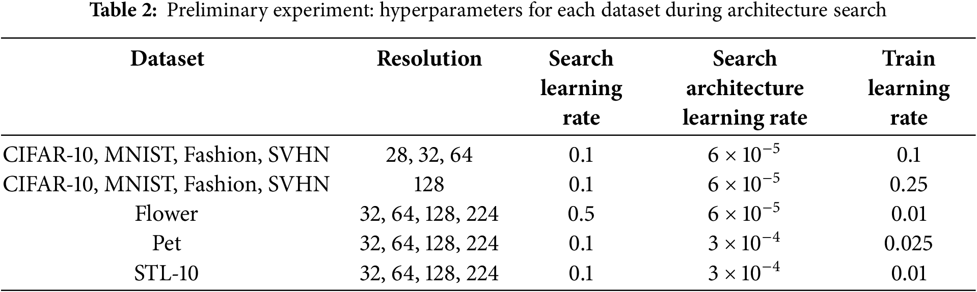
We present preliminary experiments conducted to use the dataset encoder and dimensionality reduction methods in the NAVIGATOR.

4.1 Experimental Settings of Datasets

In this experiment, we employed PC-DARTS to analyze the effects of the architectures obtained from multiple datasets. In deep learning, it has been shown that when the input image resolutions differ, lower resolution leads to decreased recognition accuracy [56]. However, in NAS–which searches for the architecture itself, there is still insufficient analysis of how image resolution affects the network architecture. Therefore, we prepared multiple datasets with varying image resolutions to evaluate their effects on the architecture.

In this experiment, seven datasets were used for analysis: CIFAR-10 [57], MNIST [58], Fashion-MNIST [59], SVHN [60], Oxford-IIIT Pet [61], Oxford 102 Flower [62], and STL-10 [63]. Because each dataset comprises images with different characteristics, we conducted experiments using multiple datasets. Table 1 presents the characteristics of the datasets.

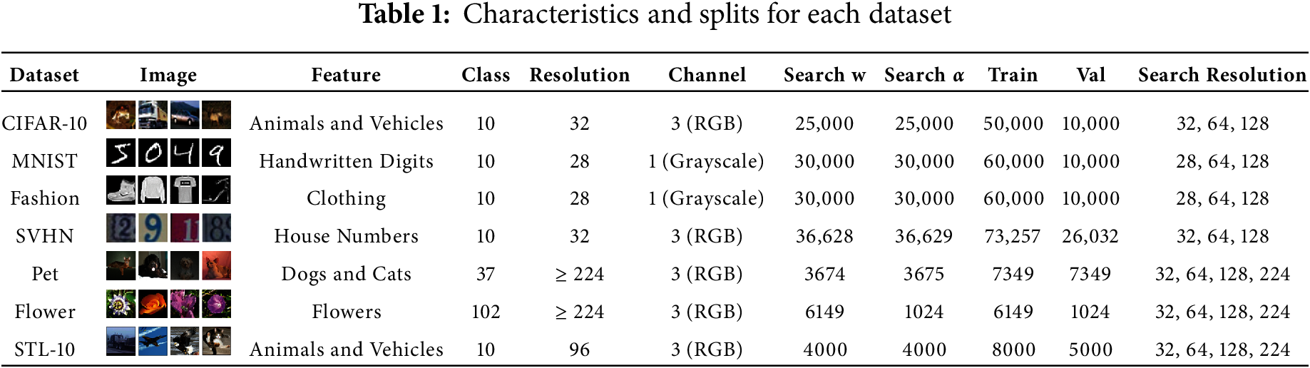
CIFAR-10 and STL-10 datasets contained visually similar images, whereas both the MNIST and Fashion-MNIST were grayscale image datasets. In addition, both MNIST and SVHN consisted of digit images. If the two datasets share similar image features, the architectures derived from PC-DARTS are expected to exhibit similar characteristics. Moreover, the Flower, Pet, and STL-10 were datasets with larger original image sizes compared with the others. To ensure consistency, downsampling was applied to reduce the image resolution according to the evaluation requirements. We hypothesized that using upsampling and downsampling yields different architectural characteristics during resolution evaluation. Hence, we included Flower, Pet, and STL-10 in the datasets. We searched for network architectures with PC-DARTS using seven datasets: CIFAR-10, MNIST, Fashion-MNIST, SVHN, Oxford-IIIT Pet, Oxford 102 Flower, and STL-10. Additionally, multiple resolutions were used for each dataset. Table 1 lists the number of images used in each subset of the dataset and the resolutions used for the exploration. Search w indicates the number of images used to learn network weights during the search phase, while Search α denotes the number of images used to learn the architecture itself. As the memory capacity required for the search process varies depending on the resolution and number of images per dataset, we altered the resolution for each of the datasets used in the experiments. Moreover, we varied the seed and repeated the architecture search four times for each resolution, because the initial network values (seeds) might introduce bias. This approach enabled us to assess the reliability and stability of the experimental results. To accurately evaluate the effects of the datasets and resolutions on the architectures, we maintained constant hyperparameters for each dataset and resolution. We determined the hyperparameters by referring to the image resolutions and the original PC-DARTS paper. Table 2 lists the learning rate and architecture learning rates applied during the architecture search.

4.2 Results and Discussion

In PC-DARTS, the term “search” refers to exploring both network connectivity patterns and types of operations. We hypothesized that different operations would be selected depending on the dataset and resolution. We counted the number of times each operation was selected for the resulting architectures. Comparing these counts across resolutions and datasets enables a more comprehensive characterization of the architectures. We summed the operations in both the Normal and the Reduction cells and then took the average over four trials.

Fig. 3 shows a stacked bar chart of the operations comprising the obtained architectures. from PC-DARTS, categorized by dataset and resolution. In CIFAR-10, MNIST, Fashion-MNIST, and SVHN, which underwent upsampling, we observed that as the resolution increased, separable convolutions decreased, and the dilated convolutions increased. In addition, within each convolution type, the share of 3×3 filters decreased, whereas 5×5 filters became more prevalent. Separable convolutions were more efficient in their operations, whereas dilated convolutions were designed to cover a larger receptive field. During upsampling, the image size increased while retaining the same overall information. Consequently, using narrow convolutions yielded fewer extracted features. Therefore, under upsampling conditions, dilated convolutions and 5×5 filters tended to be selected more often because they cover a wider area. However, in Flower, Pet, and STL-10 (where downsampling was predominant), changes in resolution did not significantly affect the chosen operations. These findings suggest that the total amount of information in the entire image has a limited effect on the number of operations required. Instead, the density of image information seems to influence the spatial range of the extracted features.

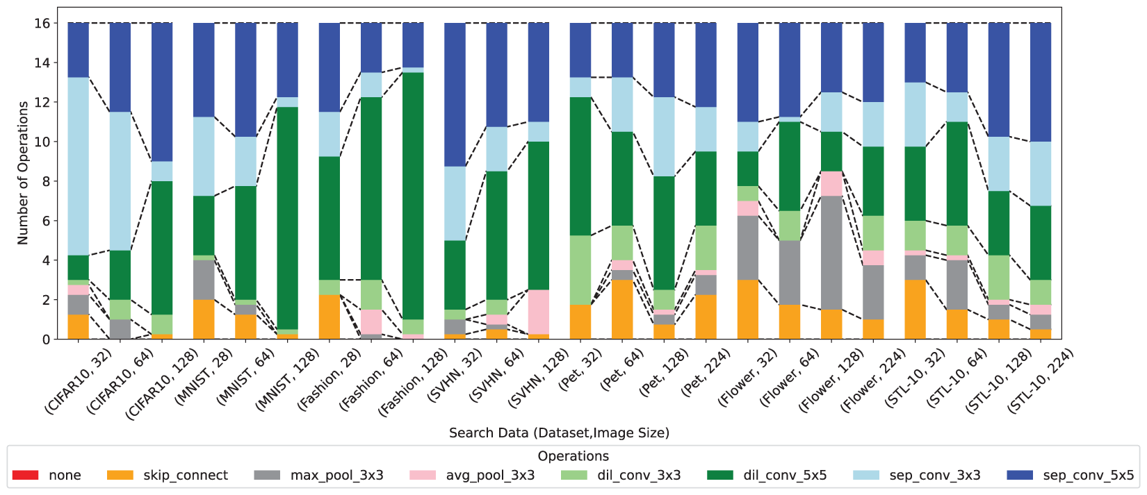
Figure 3: Number of operations for each architecture obtained from PC-DARTS

The ratio of the frequently selected operations varied depending on the dataset. In the MNIST and Fashion-MNIST datasets, a 5×5 dilated convolution was frequently used. A possible reason for this is that both datasets contained images from a single channel. Compared with datasets containing three channels, those with fewer channels provided less information in the channel dimension, leading to the selection of a 5×5 dilated convolution, which processes a broader spatial area.

Fig. 4 illustrates the latent features of each architecture derived from the NAVIGATOR. The axes represent the coordinates in the 2D PCA plot. The latent features of architectures from the same datasets (same color) tended to cluster together. For some dataset types, even different datasets distribute their latent features in adjacent regions. Moreover, latent features of architectures from CIFAR10 and STL-10 lie close to each other. One possible explanation is that CIFAR-10 (airplanes, birds, cars, cats, deer, dogs, horses, frogs, ships, and trucks) and STL-10 (airplanes, birds, cars, cats, bears, dogs, horses, monkeys, ships, truck) share eight out of ten labels. They are thus highly similar datasets, differing only in “deer/frog” versus “bear/monkey.” This similarity likely results in similar architectures. Additionally, architectures from MNIST and Fashion-MNIST clustered closely in the latent space. Both datasets have only one channel, which probably causes them to converge toward similar architectures. The flower lies in a distinct region apart from the other datasets, indicating that its architectures also diverged significantly from the others, consistent with the operation count analysis.

Figure 4: NAVIGATOR results with latent features of the architecture color-coded by dataset (legend: dataset-resolution)

Our preliminary results confirmed that the optimal architecture varies depending on the dataset— particularly when the datasets share similar labels or have the same number of channels. Accordingly, in the navigator dataset encoder of NAVIGATOR, we define dataset features that can capture these properties.

4.3 Experiments on Dimensionality Reduction

To determine the latent space for visualization, we first applied several representative dimensionality reduction methods–PCA, t-SNE [64], UMAP [65], Isomap [66], MDS [67], and LLE [68]. We projected training data into two dimensions and represented the results in Fig. 5. Note that the latent space used in this experiment was derived from the results in the following section, and the current findings were used purely to compare the different dimensionality reduction methods. In the figure, red and green points represent samples from different classes. We observed similar but slightly varying patterns of dispersion and similarity among the different methods.

Figure 5: Comparison of dimensionality reduction results from PCA, t-SNE, UMAP, Isomap, MDS, and LLE

Based on this comparison, we used PCA in this study. The main reasons for this are as follows: (1) PCA constructs the latent space through linear transformations, making it conceptually compatible with the VGAE latent representation and highly interpretable; (2) compared to other methods, PCA facilitates a clearer visual understanding of inter-class distribution patterns.

5  Experiments

This study evaluated the effectiveness of the proposed method through experiments that use multiple, distinct datasets. To determine the optimal architecture for each dataset, we adopted PC-DARTS as the NAS component of NAVIGATOR. PC-DARTS delivers high accuracy quickly, making it an ideal choice for our experiments, which require testing of multiple architectures. Moreover, the PC-DARTS search spaces encompassed approximately 1025 possible architectures. Its efficiency and large scale make it ideal under our experimental conditions. In each trial, we used a single NVIDIA Tesla V100 SXM2 16 GB GPU (four such GPUs were employed in parallel for ImageNet).

5.1 Experiment I: Visualizing the Output from Latent Features

The objective of Experiment I was to verify whether architectures with similar characteristics can be generated from the latent feature space extracted by the NAVIGATOR. Next, we describe the results obtained by adding noise around the specified feature vectors to observe the shapes of model architectures distributed nearby. This experiment used two datasets: CIFAR-10 and MNIST. Based on the insight that latent features encompass dataset-specific properties, we used the latent features extracted by NAVIGATOR from an architecture optimized for CIFAR-10 and then fine-tuned them. This approach demonstrated that various architectures similar to the original output graph can be generated. In addition, learning an architecture that connects two types of cells rather than the entire graph can extract more detailed features and facilitate easier visualization of the graph.

Fig. 6 shows a graph of the input architecture and a graph generated from the latent features. The input nodes are shown in blue, the middle nodes in orange, and the output nodes in green. The number of edges matched that of the input graph.

Figure 6: Graphs generated from input graphs and latent features

First, we observed that the original graph (a) and reconstruction graph (b) are the same. This finding confirms that the NAVIGATOR encoder and decoder can reconstruct architecture with high fidelity. Next, when examining the changes in the small perturbation parameter γ, we find that at γ=0.05 in (d), two edges differ from the original. However, the overall architecture remains significantly similar to the original graph (a) up through (h), also at γ=0.05.

When generating new latent features, we follow the Generating Model algorithm described in Section 3.6, which first normalizes the features into the range [0, 1].

Moreover, the direction vector multiplied by γ is fixed at unit length; therefore, a small perturbation of γ=0.05 results in an approximately 5% shift from the original values in the latent feature space. This small change explains why the generated architecture in Fig. 6 remains almost identical to the original architecture.

However, for γ=0.1 and higher, the overall architecture gradually changes while retaining its fundamental features. Notably, the labels for certain edges (represented by colors) differ, indicating that the edge features shifted. Basically, increasing γ enables the free generation of new architectures with characteristics that diverge from the original graph.

Furthermore, in the proposed method, certain constraints are imposed during NAS-based architecture generation. For instance, the number of edges that could connect to each middle node (e.g., nodes 2–5 and 9–12) was fixed at two. Additionally, we merged normal and reduced cells per plot, respectively. This setup includes certain mandatory fixed edges (for example, from Node 1 to Node 7 or output edges) while restricting unconstrained connections within the cells. We introduced these rules to replicate the search space used in DARTS and PC-DARTS. For a fair comparison, we applied the same conditions as those used for the input architecture. Note that these constraints can be relaxed if the objective is to generate diverse architectures.

Fig. 7 shows the color map of the architecture generated by the proposed method, where the vertical axis is the value of γ and the horizontal axis is the same γ value to generate direction vectors from five times uniform random numbers. The colors represent edge-connection operations sorted from the top in order of proximity to the input node from the left. Architectures of the model are relatively unchanged except for γ = 1.0, and γ = 0.0 remains unchanged (because the feature points did not move), and both the vertical and horizontal directions changed as the value increased. As shown in Fig. 7, these parameters are linked to the architectural changes. When γ = 1.0, more purple operations (skip connections) were accepted, indicating that the architectures of the space away from the learned architectures were biased. Biased architectures are built because normalization and moving the latent features by as much as 1.0 will generate them outside the latent space.

Figure 7: Color representation of operations for each architecture. The vertical axis is the value of γ and the horizontal axis is the same γ value to generate direction vectors from five times uniform random numbers. Edge connections are not considered. γ = 0 is the original and reconstructed architecture. None: red, max pooling 3 × 3: green, average pooling 3 × 3: blue, skip connection: purple, separable convolution 3 × 3: orange, separable convolution 5 × 5: brown, dilated convolution 3 × 3: pink, dilated convolution 5 × 5: gray (same as edge colors in Fig. 6)

5.2 Experiment II: Experimental Settings for the Latent Feature Visualization of Architecture Searched in CIFAR-10 and MNIST

In Experiment II, we aimed to obtain architectures optimized by NAS for two datasets with different properties and then visualize the latent features of the network architectures adapted to each dataset. In NAVIGATOR, we hypothesized that the model inputs to VGAE would be distributed in different regions of the latent space, depending on the dataset. We conducted experiments to verify this hypothesis. In the experiment, we used two datasets: CIFAR-10 and MNIST. Each architecture includes both connection patterns and types of edges, whereas the number of nodes remained fixed at. Using five different seed values, we obtained ten architectures. During the search phase, 50 epochs were used for training. The learning rate was decreased from 0.1 to 0 according to a cosine schedule, the architecture parameter learning rate was set to 0.0003, and random cropping and horizontal flipping were applied for data augmentation. For the VGAE configuration, 500,000 epochs were used. The learning rate decreased from 0.001 to 0.00025 following a cosine schedule, and Adam was used as the optimizer. Dimensions of latent features were set to four based on a seed value of 2024. We also adjusted the loss function weights WP, WN, WEdge, and WKL to 2.0, 1.0, 0.5, and 1.0, respectively. These hyperparameters were chosen by referring to original papers on NAS methods and VGAE.

5.3 Experiment II: Results and Discussion

Fig. 8 shows the visualization results of the latent features obtained using the proposed method. This figure illustrates dimensionality reduction using PCA. Each axis corresponds to a coordinate derived by compressing high-dimensional data. Owing to the differences in the image size and dataset characteristics of CIFAR-10 (RGB) and MNIST (grayscale), the NAS procedure is likely to be identified as optimized architectures to capture the distinctive features of each dataset. Moreover, CIFAR-10 has an input size of 32 × 32, whereas MNIST is 28 × 28, leading to different optimal latent features for each dataset. Consequently, distinct trends were observed between the two.

Figure 8: Visualization of latent features acquired using the proposed method. The axes represent the coordinate axes on a two-dimensional PCA plot

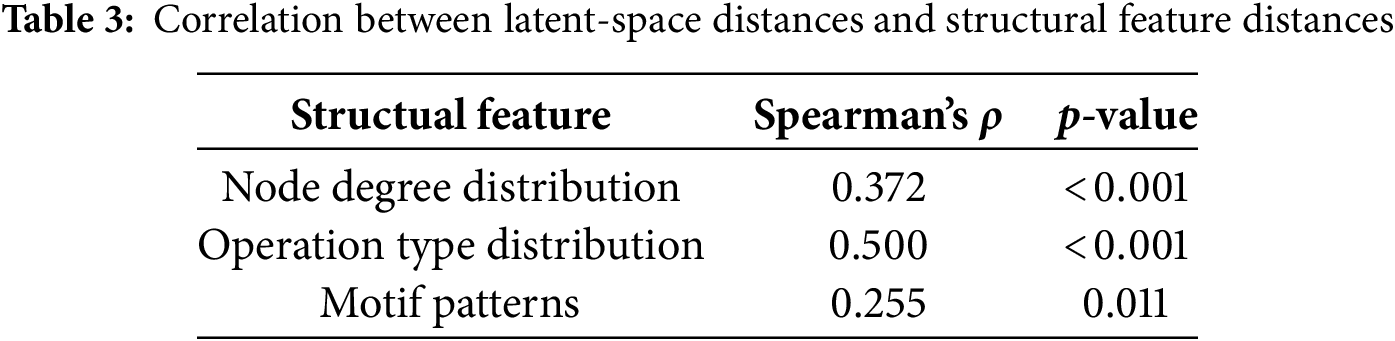
To gain a deeper understanding of how the latent space preserves the graph-structural features of neural architectures, we conducted a correlation analysis between inter-architecture distance in the latent space and the distances of their structural features. Specifically, we used the following representative structural features: (1) the degree distribution of node connections, (2) the distribution of operation types, and (3) motif patterns, defined as the frequency of three-node subgraphs. For each pair of architectures, we computed the distance between these features using the Kullback–Leibler divergence. Then we assessed the relationship between the structural and the latent-space distance by calculating the Spearman correlation coefficient. The results are presented in Table 3. Among the examined structural features, the distribution of operation types shows the strongest correlation with latent-space distances, while the degree distribution indicates a moderate correlation. Although the motif pattern correlation is comparatively weaker, it remains a significantly positive correlation, suggesting that certain structural patterns are effectively captured. These findings suggest that the proposed method successfully preserves the topological properties of neural architectures within the latent space. In other words, the method constructs a latent space that maintains consistency in both semantic meaning and structural aspects.

Overall, training the VGAE in NAVIGATOR (for ten architectures over 500,000 epochs) required 14.52 h. Meanwhile, the NAS phase using standard PC-DARTS required approximately 2.4 h of training time per architecture. Hence, by prebuilding a large latent space optimized for multiple datasets, we demonstrate that the proposed method can generate architectures for new datasets in a short amount of time. This highlights the effectiveness of the proposed approach.

5.4 Experiment III: Experimental Settings for Performance Test of Generated Architecture in NAVIGATOR

In Experiment III, we compared the architectures generated by NAVIGATOR with those generated randomly on the USPS and ImageNet datasets. We aimed to evaluate whether the proposed method can produce promising architectures and whether it offers performance improvements over random generations. The newly introduced USPS (United States Postal Service) dataset [69] contains 16 × 16 grayscale images of handwritten digits from 0 to 9. It is frequently used as a domain adaptation example based on MNIST [70–72]. Hence, we investigated whether an architecture optimized for a similar dataset can achieve comparable performance to the USPS. We retrained and evaluated four types of architectures for their accuracy. The first architecture is generated from latent features around MNIST (γ=0.1). The second architecture is generated from latent features around CIFAR-10 (γ=0.1). The third and fourth architectures are generated from the MNIST (γ=0.0) and random latent features, respectively. Based on the results of Experiment I, we set γ=0.1 as the parameter for building latent features around the original. While it retains the characteristics of the γ=0.0 architecture, it also produces partially different architectures. For both MNIST and CIFAR-10 datasets, five sets of latent features exist. We generated the directional vectors four times (using random values) to construct each model. In total, we evaluated 50 architectures across the four types. To retrain the USPS, we set the number of training epochs to 600 with a batch size of 128. The initial learning rate was 0.025 (reduced to zero following a cosine schedule), momentum was 0.9, weight decay was 3×10−4, drop path probability was 0.3, and we employed cutout.

Evaluating NAVIGATOR’s effectiveness of NAVIGATOR for datasets with larger image sizes is crucial, given that the USPS images are only 16 × 16. Therefore, additional experiments were conducted using the ImageNet dataset in Experiment III as well. ImageNet is a widely used dataset for image classification [73]. Among the underlying PC-DARTS approaches, the models discovered on CIFAR-10 were transferred to ImageNet. In Experiment III, 20 architectures generated from latent features around CIFAR-10 were evaluated on ImageNet. As the ImageNet images were originally large, they were cropped to 224 × 224 pixels. We also used RandomHorizontalFlip (for random left-right flips) and ColorJitter (for random changes in brightness and contrast) for data augmentation. Computations were parallelized across four GPUs. For the ImageNet retraining, we used 250 epochs, a batch size of 768, and an initial learning rate of 0.5 (reduced to zero using a linear schedule). Momentum was set to 0.9, and weight decay was 3×10−5. In addition, label smoothing and a five-epoch warm-up phase were employed. For simplicity, the auxiliary loss was not applied. We selected the hyperparameters for retraining on ImageNet and USPS by referring to the original PC-DARTS study. Fig. 9 presents examples of architectures (MNIST Model and CIFAR-10 Model) generated by the proposed method and used for evaluation in Experiment III.

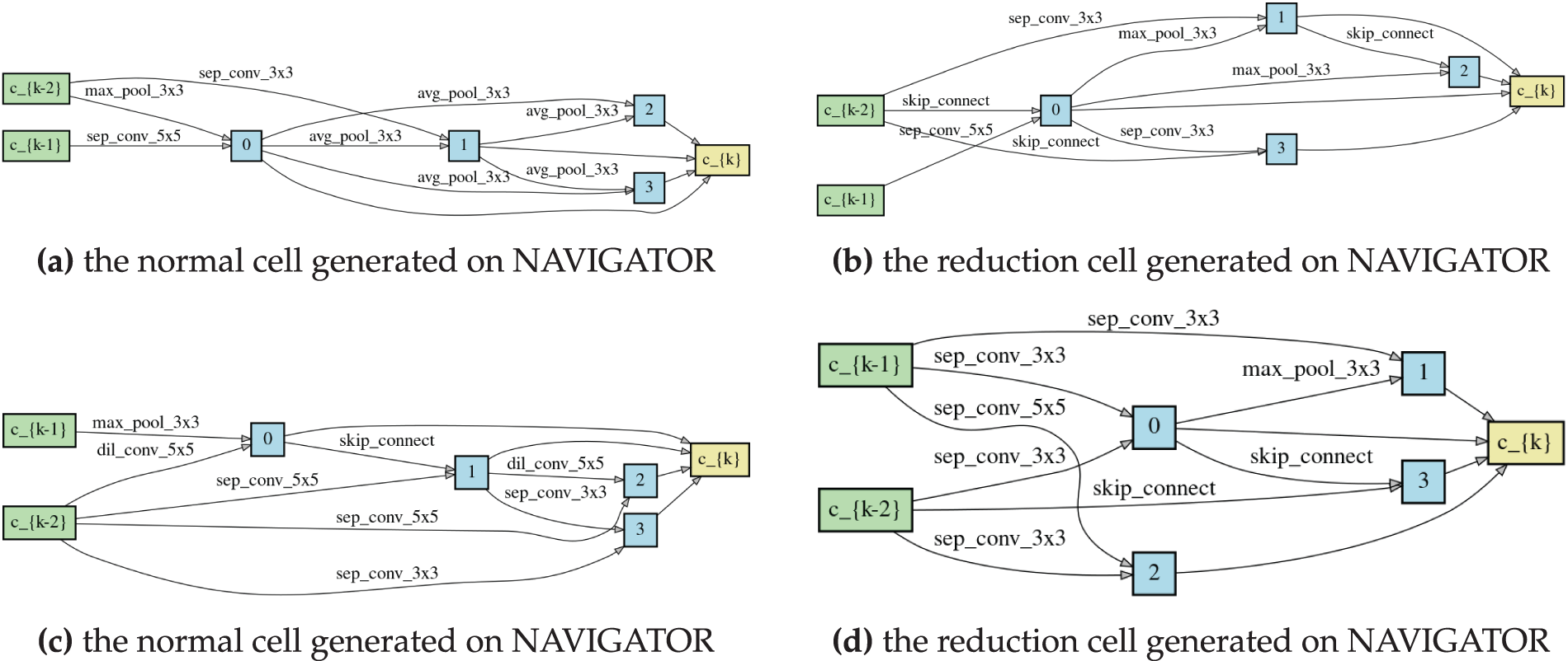
Figure 9: Example of an architecture generated by NAVIGATOR. The upper figures are MNIST models and the lower figures are CIFAR-10 models

5.5 Experiment III: Results and Discussion

Table 4 presents the results of each NAS method. From Table 4, we can see that the MNIST Model (γ=0.1), which reached a best test accuracy (Max) of 98.11%, achieved the highest accuracy. Basically, the architecture constructed by referring to the latent features optimized on a similar dataset produced the best results. Furthermore, the MNIST Model achieved a higher performance than both the random and CIFAR-10 models. Even within the same MNIST Model, the variant with γ=0.1 outperformed the variant with γ=0.0. This finding demonstrates the usefulness of our perturbation-based method. When γ=0.0, the architecture was originally optimized for MNIST; however, despite its similarity to USPS, USPS retains characteristics, making the perturbed approach beneficial. As the same technique can be applied to new datasets, NAS does not require to be conducted from scratch. This leads to a significant reduction in the search time. Moreover, in the ImageNet experiment results shown in Fig. 10, we found that the NAVIGATOR approach (CIFAR-10 Model, γ=0.1) achieved the highest accuracy, recording a Best Test Acc. (Max) of 75.43% in Top-1 and 92.60% in Top-5. Moreover, in the ImageNet experiment results shown in Fig. 10, we found that the NAVIGATOR approach (CIFAR-10 Model, γ=0.1) achieved the highest accuracy, recording a Best Test Acc.(Max) of 75.43% for Top-1 and 92.60% in Top-5. In a Mobile Setting where FLOPs were below 600 M, PC-DARTS achieved the highest accuracy; however, the architecture generated by NAVIGATOR remains competitive at a similar performance level. Hence, our proposed method can still produce a set of architectures with rival approaches even under relatively low-FLOPs conditions. Moreover, achieving high performance while drastically reducing the search time represents a major advantage of our method. These experimental results clearly demonstrate that the proposed method remains effective on datasets with large image sizes and large-scale architectures constructed via Cell transfer.

5.6 Experiment IV: Performance Test of Un-Architecture Information Encoder

In Experiment IV, we experimented using an extended version of NAVIGATOR that can incorporate Un-architectural information into latent features. Subsequently, we evaluated their effectiveness. We used CLIP for dataset features and ResNet18 for task features. Details of the methodology and the model generation procedure are described in Sections 3.5 and 3.6. For our experimental setup, we built the latent feature space using CIFAR-10, and MNIST (as in Experiments I–III) and tested it on the USPS dataset, which serves as a previously unseen problem.

Fig. 11 visualizes the latent feature spaces obtained in four scenarios: (1) architecture features alone, (2) additional dataset features, (3) additional task features, and (4) both datasets and task features. This figure shows the results of dimensionality reduction using PCA, where each axis corresponds to a coordinate representing the compressed multidimensional data. From these results, we observed a particularly pronounced separation when the dataset features were included. However, when task features were included, significant clustering did not emerge, suggesting that the influence or differences introduced by task features are relatively small.

Figure 11: Visualization of latent features acquired using the proposed method. The axes represent the coordinate axes on a two-dimensional PCA plot

Table 5 presents the model sizes and test accuracies achieved by each architecture on the USPS dataset. Normal refers to the MNIST Model (γ=0.1) which produced the highest evaluation results in Experiment III. This table confirms that NAVIGATOR, incorporating dataset features achieved the highest performance. We believe that the experimental results are highly dependent on the chosen datasets and tasks. In this case, the USPS dataset is grayscale and more similar to MNIST than to CIFAR-10. Consequently, the newly generated latent features likely placed a stronger emphasis on the MNIST, producing architectures similar to the MNIST Model, thus yielding higher performance. In contrast, architectures incorporating task features exhibited lower performance. We suspect this was because significantly distinguishing gradients were not discovered during the design of the task features. As demonstrated by our experiment, the construction of an appropriate encoder is crucial for performance improvement. Embedding unarchitectured information–previously unaddressed by architecture feature extraction–into the same space for exploration is a major advantage of NAVIGATOR.

6  Conclusion

This study proposed NAVIGATOR, a framework that integrates NAS and VGAE to significantly reduce search time. Additionally, by extracting features from datasets and tasks, we introduced a method to measure distances among different datasets or tasks. This advancement further refined the optimization process within the latent feature space. A future direction involves extending the proposed method to generate similar architectures in search spaces beyond those covered by currently trained models. This limitation arises from the fact that NAVIGATOR’s performance may be constrained by the diversity of the initial set of architectures used during the training phase. In addition, the dataset and task feature embeddings employed in this study may be insufficient for capturing subtle distinctions between tasks, indicating the need for more accurate and efficient embedding methods in future work. Furthermore, extending NAVIGATOR to accommodate dynamically changing search spaces and user-specified constraints can evolve it practically and flexibly, enabling an approach for multi-objective searches. This approach promises to navigate toward advances in neural architecture search and foster deeper insights into the realm of network design and optimization.

Acknowledgement: Not applicable.

Funding Statement: This research was funded by the New Energy and Industrial Technology Development Organization (NEDO), grant number JPNP18002.

Author Contributions: The authors confirm contribution to the paper as follows: Conceptualization, Kazuki Hemmi; methodology, Kazuki Hemmi, Yuki Tanigaki and Kaisei Hara; data curation, Kazuki Hemmi; writing—original draft preparation, Kazuki Hemmi; writing—review and editing, Kazuki Hemmi, Yuki Tanigaki, Kaisei Hara and Masaki Onishi. All authors reviewed the results and approved the final version of the manuscript.

Availability of Data and Materials: The datasets used in this study are available from the authors upon reasonable request. The experimental dataset was obtained from torchvision.datasets, and several models were sourced from Hugging Face.

Ethics Approval: Not applicable.

Conflicts of Interest: The authors declare no conflicts of interest to report regarding the present study.

References

1. Kipf TN, Welling M. Semi-supervised classification with graph convolutional networks. arXiv:1609.02907. 2016. [Google Scholar]

2. Hemmi K, Tanigaki Y, Onishi M. NAVIGATOR-D3: neural architecture search using variational graph auto-encoder toward optimal architecture design for diverse datasets. In: International Conference on Artificial Neural Networks; 2024 Sep 17–20; Lugano, Switzerland; 2024. p. 292–307. [Google Scholar]

3. Zoph B, Le QV. Neural architecture search with reinforcement learning. In: ICLR 2017; 2017 Apr 24–26; Toulon, France. [Google Scholar]

4. Xu Y, Jia Z, Wang LB, Ai Y, Zhang F, Lai M, et al. Large scale tissue histopathology image classification, segmentation, and visualization via deep convolutional activation features. BMC Bioinform. 2017;18(1):1–17. doi:10.1186/s12859-017-1685-x. [Google Scholar] [PubMed] [CrossRef]

5. Liu H, Simonyan K, Vinyals O, Fernando C, Kavukcuoglu K. Hierarchical representations for efficient architecture search. arXiv:1711.00436. 2017. [Google Scholar]

6. Real E, Moore S, Selle A, Saxena S, Suematsu YL, Tan J et al. Large-scale eolution of image classifiers. In: Proceedings of the 34th International Conference on Machine Learning; 2017 Aug 6–11; Sydney, NSW, Australia; 2017. p. 2902–11. [Google Scholar]

7. Liu H, Simonyan K, Yang Y. Darts: differentiable architecture search. arXiv:1806.09055. 2018. [Google Scholar]

8. Xu Y, Xie L, Zhang X, Chen X, Qi G, Tian Q, et al. PC-DARTS: partial channel connections for memory-efficient architecture search. In: 2020 International Conference on Learning Representations; 2020 Apr 30; Ethiopia: Addis Ababa. p. 1–13. [Google Scholar]

9. Wong C, Houlsby N, Lu Y, Gesmundo A. Transfer learning with neural AutoML. In: NIPS’18: Proceedings of the 32nd International Conference on Neural Information Processing Systems; 2018 Dec 3–8; Montreal, QC, Canada. p. 8366–75. [Google Scholar]

10. Xue Y, Han X, Wang Z. Self-adaptive weight based on dual-attention for differentiable neural architecture search. IEEE Trans Indus Inform. 2024;20(4):6394–403. doi:10.1109/tii.2023.3348843. [Google Scholar] [CrossRef]

11. Chen M, Peng H, Fu J, Ling H. Autoformer: searching transformers for visual recognition. In: Proceedings of the 2021 IEEE/CVF International Conference on Computer Vision; 2021 Oct 11–17; Montreal, QC, Canada. p. 12270–80. [Google Scholar]

12. Chen M, Wu K, Ni B, Peng H, Liu B, Fu J et al. Searching the search space of vision transformer. Adv Neural Inform Process Syst. 2021;34:8714–26. [Google Scholar]

13. Nasir MU, Earle S, Togelius J, James S, Cleghorn C. LLMatic: neural architecture search via large language models and quality diversity optimization. In: Proceedings of the 2024 Genetic and Evolutionary Computation Conference; 2024 Jul 14–18; Melbourne, VIC, Australia. p. 1110–8. [Google Scholar]

14. Zheng M, Su X, You S, Wang F, Qian C, Xu C et al. Can GPT-4 perform neural architecture search? arXiv: 2304.10970. 2023. [Google Scholar]

15. Scarselli F, Gori M, Tsoi AC, Hagenbuchner M, Monfardini G. The graph neural network model. IEEE Trans Neural Netw. 2008;20(1):61–80. doi:10.1109/tnn.2008.2005605. [Google Scholar] [PubMed] [CrossRef]

16. Jiang D, Wu Z, Hsieh CY, Chen G, Liao B, Wang Z, et al. Could graph neural networks learn better molecular representation for drug discovery? A comparison study of descriptor-based and graph-based models. J Cheminform. 2021;13(1):12. doi:10.21203/rs.3.rs-79416/v1. [Google Scholar] [CrossRef]

17. Wang X, Flannery ST, Kihara D. Protein docking model evaluation by graph neural networks. Front Mol Biosci. 2021;8(Suppl 1):647915. doi:10.1101/2020.12.30.424859. [Google Scholar] [CrossRef]

18. Sanchez-Gonzalez A, Godwin J, Pfaff T, Ying R, Leskovec J, Battaglia PW. Learning to simulate complex physics with graph networks. In: Proceedings of the 2020 International Conference on Machine Learnin; 2020 Jul 13–18; Online. p. 8459–68. [Google Scholar]

19. Shlomi J, Battaglia P, Vlimant JR. Graph neural networks in particle physics. Mach Learn Sci Technol. 2020;2(2):021001. doi:10.1088/2632-2153/abbf9a. [Google Scholar] [CrossRef]

20. Velickovic P, Cucurull G, Casanova A, Romero A, Liò P, Bengio Y. Graph attention networks. In: The 6th International Conference on Learning Representations; 2018 Apr 30–May 3; Vancouver, BC, Canada. p. 1–12. [Google Scholar]

21. Hamilton W, Ying Z, Leskovec J. Inductive representation learning on large graphs. Adv Neural Inform Process Syst. 2017;30:1025–35. [Google Scholar]

22. Defferrard M, Bresson X, Vandergheynst P. Convolutional neural networks on graphs with fast localized spectral filtering. Adv Neural Inf Process Syst. 2016;29:3844–52. [Google Scholar]

23. Xu K, Hu W, Leskovec J, Jegelka S. How powerful are graph neural networks? arXiv:1810.00826. 2018. [Google Scholar]

24. Kipf TN, Welling M. Variational graph auto-encoders. arXiv:1611.07308. 2016. [Google Scholar]

25. Kingma DP, Welling M. Auto-encoding variational bayes. arXiv:1312.6114. 2013. [Google Scholar]

26. Cappart Q, Chételat D, Khalil EB, Lodi A, Morris C, Veličković P. Combinatorial optimization and reasoning with graph neural networks. J Mach Learn Res. 2023;24(130):1–61. [Google Scholar]

27. Almasan P, Suárez-Varela J, Rusek K, Barlet-Ros P, Cabellos-Aparicio A. Deep reinforcement learning meets graph neural networks: exploring a routing optimization use case. Comput Commun. 2022;196(4):184–94. doi:10.1016/j.comcom.2022.09.029. [Google Scholar] [CrossRef]

28. Zoph B, Vasudevan V, Shlens J, Le QV. Learning transferable architectures for scalable image recognition. In: Proceedings of the IEEE/CVF Conference on Computer Vision and Pattern Recognition; 2018 Jun 18–23; Salt Lake City, UT, USA. p. 8697–710. [Google Scholar]

29. Mellor J, Turner J, Storkey A, Crowley EJ. Neural architecture search without training. In: 2021 International Conference on Machine Learning; 2021 Jul 18–24; Online. p. 7588–98. [Google Scholar]

30. Krishnakumar A, White C, Zela A, Tu R, Safari M, Hutter F. NAS-Bench-Suite-Zero: accelerating research on zero cost proxies. Adv Neural Inform Process Syst. 2022;35:28037–51. [Google Scholar]

31. Friede D, Lukasik J, Stuckenschmidt H, Keuper M. A variational-sequential graph autoencoder for neural architecture performance prediction. arXiv:1912.05317. 2019. [Google Scholar]

32. Yan S, Zheng Y, Ao W, Zeng X, Zhang M. Does unsupervised architecture representation learning help neural architecture search?. In: NIPS’20: 34th International Conference on Neural Information Processing Systems; 2020 Dec 6–12; Vancouver, BC, Canada. [Google Scholar]

33. Ning X, Zheng Y, Zhao T, Wang Y, Yang H. A generic graph-based neural architecture encoding scheme for predictor-based NAS. In: Proceedings of European Conference on Computer Vision; 2020 Aug 23–28; Glasgow, UK. p. 189–204. [Google Scholar]

34. Lee H, Hyung E, Hwang SJ. Rapid neural architecture search by learning to generate graphs from datasets. arXiv:2107.00860. 2021. [Google Scholar]

35. Chatzianastasis M, Dasoulas G, Siolas G, Vazirgiannis M. Graph-based neural architecture search with operation embeddings. In: Proceedings of the IEEE/CVF International Conference on Computer Vision Workshops; 2021 Oct 11–17; Montreal, BC, Canada. p. 393–402. [Google Scholar]

36. Lukasik J, Friede D, Zela A, Hutter F, Keuper M. Smooth variational graph embeddings for efficient neural architecture search. In: 2021 International Joint Conference on Neural Networks (IJCNN); 2021 Jul 18–22; Shenzhen, China. p. 1–8. [Google Scholar]

37. Suchopárová G, Neruda R. Graph embedding for neural architecture search with input-output information. In: AutoML Conference Workshop Track; 2022; Baltimore, MD, USA. [Google Scholar]

38. Wen W, Liu H, Chen Y, Li H, Bender G, Kindermans P. Neural Predictor for Neural Architecture Search. In: Proceedings of European Conference on Computer Vision; 2020 Aug 23–28; Glasgow, UK. p. 660–76. [Google Scholar]

39. Chen Y, Guo Y, Chen Q, Li M, Zeng W, Wang Y, et al. Contrastive neural architecture search with neural architecture comparators. In: Proceedings of the 2021 IEEE/CVF Conference on Computer Vision and Pattern Recognition; 2021 Jun 20–25; Nashville, TN, USA. p. 9502–11. [Google Scholar]

40. White C, Neiswanger W, Savani Y. BANANAS: bayesian optimization with neural architectures for neural architecture search. Proc AAAI Conf Artif Intell. 2021;35(12):10293–301. doi:10.1609/aaai.v35i12.17233. [Google Scholar] [CrossRef]

41. Lukasik J, Jung S, Keuper M. Learning where to look-generative NAS is surprisingly efficient. arXiv:2203.08734. 2022. [Google Scholar]

42. Agiollo A, Omicini A. GNN2GNN: graph neural networks to generate neural networks. In: Proceedings of the Thirty-Eighth Conference on Uncertainty in Artificial Intelligence; 2022 Aug 1–5; Eindhoven, The Netherlands. p. 32–42. [Google Scholar]

43. Dudziak L, Chau T, Abdelfattah MS, Lee R, Kim H, Lane ND. BRP–NAS: prediction-based NAS using GCNs. Adv Neural Inform Process Syst. 2020;33:10480–90. [Google Scholar]

44. Shi H, Pi R, Xu H, Li Z, Kwok JT, Zhang T. Bridging the gap between sample-based and one-shot neural architecture search with bonas. Adv Neural Inform Process Syst. 2020;33:1808–19. [Google Scholar]

45. Wistuba M. XferNAS: transfer neural architecture search. In: Machine Learning and Knowledge Discovery in Databases: European Conference; 2021 Sep 13–17; Bilbao, Spain. p. 247–62. [Google Scholar]

46. Singamsetti M, Mahajan A, Guzdial M. Conceptual expansion neural architecture search (CENAS). arXiv:2110.03144. 2021. [Google Scholar]

47. Lu Z, Sreekumar G, Goodman E, Banzhaf W, Deb K, Boddeti VN. Neural architecture transfer. arXiv:2005.05859. 2020. [Google Scholar]

48. Luo R, Tian Fei, Qin Tao, Chen E, Liu T-Y. Neural architecture optimization. Adv Neural Inform Process Syst. 2018;31:7816–27. [Google Scholar]

49. Li J, Liu Y, Liu J, Wang W. Neural architecture optimization with graph VAE. arXiv:2006.10310. 2020. [Google Scholar]

50. Pearson KLIII. On lines and planes of closest fit to systems of points in space. London Edinburgh Dublin Philosoph Magaz J Sci. 1901;2(11):559–72. doi:10.1080/14786440109462720. [Google Scholar] [CrossRef]

51. Radford A, Kim JW, Hallacy C, Ramesh A, Goh G, Agarwal S et al. Learning transferable visual models from natural language supervision. In: International Conference on Machine Learning; 2021 Jul 18–24; Online. p. 8748–63. [Google Scholar]

52. Watanabe K, Hemmi K, Onishi M. How neural architecture search optimize architecture with different task? Forum Data Eng Inform Manage. 2025. [Google Scholar]

53. He K, Zhang X, Ren S, Sun J. Deep residual learning for image recognition. In: Proceedings of the IEEE Conference on Computer Vision and Pattern Recognition; 2016 Jun 27–30; Las Vegas, NV, USA. p. 770–8. [Google Scholar]

54. Achille A, Lam M, Tewari R, Ravichandran A, Maji S, Fowlkes CC et al. Task2Vec: task embedding for meta-learning. In: Proceedings of the IEEE/CVF International Conference on Computer Vision; 2019 Oct 27–Nov 2; Seoul, Republic of Korea. p. 6430–9. [Google Scholar]

55. Ilharco G, Ribeiro MT, Wortsman M, Schmidt L, Hajishirzi H, Farhadi A. Editing models with task arithmetic. In: The Eleventh International Conference on Learning Representations; 2023 May 1–5. Kigali, Rwanda. [Google Scholar]

56. Sabottke CF, Spieler BM. The effect of image resolution on deep learning in radiography. Radiol Artif Intell. 2020;2(1):e190015. doi:10.1148/ryai.2019190015. [Google Scholar] [PubMed] [CrossRef]

57. Krizhevsky A, Hinton G. Learning multiple layers of features from tiny images [master’s thesis], Toronto, ON, Canada: Department of Computer Science, University of Toronto; 2009. [Google Scholar]

58. LeCun Y, Bottou L, Bengio Y, Haffner P. Gradient-based learning applied to document recognition. Proc IEEE. 1998;86(11):2278–324. doi:10.1109/5.726791. [Google Scholar] [CrossRef]

59. Xiao H, Rasul K, Vollgraf R. Fashion-mnist: a novel image dataset for benchmarking machine learning algorithms. arXiv:1708.07747. 2017. [Google Scholar]

60. Netzer Y, Wang T, Coates A, Bissacco A, Wu B, Ng AY. Reading digits in natural images with unsupervised feature learning. In: NIPS Workshop on Deep Learning and Unsupervised Feature Learning 2011; 2011 Dec 16; Granada, Spain. p. 1–9. doi:10.1109/icdar.2011.95. [Google Scholar] [CrossRef]

61. Parkhi OM, Vedaldi A, Zisserman A, Jawahar C. Cats and dogs. In: 2012 IEEE Conference on Computer Vision And Pattern Recognition; 2012 Jun 16–21; Providence, RI, USA. p. 3498–505. [Google Scholar]

62. Nilsback ME, Zisserman A. Automated flower classification over a large number of classes. In: 2008 Sixth Indian Conference on Computer Vision, Graphics & Image Processing; 2008 Dec 16–19; Bhubaneswar, India. p. 722–9. [Google Scholar]

63. Coates A, Ng A, Lee H. An analysis of single-layer networks in unsupervised feature learning. In: Proceedings of the Fourteenth International Conference on Artificial Intelligence and Statistics; 2011 Apr 11–13; Fort Lauderdale, FL, USA. p. 215–23. [Google Scholar]

64. Van der Maaten L, Hinton G. Visualizing data using t-SNE. J Mach Learn Res. 2008;9(86):2579–605. [Google Scholar]

65. McInnes L, Healy J, Melville J. UMAP: Uniform manifold approximation and projection for dimension reduction. arXiv:1802.03426. 2018. [Google Scholar]

66. Tenenbaum JB, Vd Silva, Langford JC. A global geometric framework for nonlinear dimensionality reduction. science. 2000;290(5500):2319–23. doi:10.1126/science.290.5500.2319. [Google Scholar] [PubMed] [CrossRef]

67. Kruskal JB. Multidimensional scaling by optimizing goodness of fit to a nonmetric hypothesis. Psychometrika. 1964;29(1):1–27. doi:10.1007/bf02289565. [Google Scholar] [CrossRef]

68. Roweis ST, Saul LK. Nonlinear dimensionality reduction by locally linear embedding. Science. 2000;290(5500):2323–6. doi:10.1126/science.290.5500.2323. [Google Scholar] [PubMed] [CrossRef]

69. Hull JJ. A database for handwritten text recognition research. IEEE Trans Pattern Anal Mach Intell. 1994;16(5):550–4. doi:10.1109/34.291440. [Google Scholar] [CrossRef]

70. Schrod S, Lippl J, Schäfer A, Altenbuchinger M. FACT: federated adversarial cross training. arXiv:2306.00607. 2023. [Google Scholar]

71. Wang J, Chen J, Lin J, Sigal L, de Silva CW. Discriminative feature alignment: improving transferability of unsupervised domain adaptation by Gaussian-guided latent alignment. Pattern Recognit. 2021;116(1):107943. doi:10.1016/j.patcog.2021.107943. [Google Scholar] [CrossRef]

72. French G, Mackiewicz M, Fisher M. Self-ensembling for visual domain adaptation. arXiv:1706.05208. 2017. [Google Scholar]

73. Russakovsky O, Deng J, Su H, Krause J, Satheesh S, Ma S, et al. Imagenet large scale visual recognition challenge. Int J Comput Vis. 2015;115(3):211–52. doi:10.1007/s11263-015-0816-y. [Google Scholar] [CrossRef]

74. Muravev A, Raitoharju J, Gabbouj M. Neural architecture search by estimation of network structure distributions. IEEE Access. 2021;9:15304–19. doi:10.1109/access.2021.3052996. [Google Scholar] [CrossRef]

75. Li Y, Peng X. Network architecture search for domain adaptation. arXiv:2008.05706. 2020. [Google Scholar]