Hierarchical Shape Pruning for 3D Sparse Convolution Networks

1  Introduction

Voxels in 3D space are encoded from the point cloud, which is manifested in the form of regular 3D grids. Influenced by the sparsity of the point cloud, voxels also exhibit sparse distribution in 3D space, and when extracting voxel features, the traditional 3D convolution will require substantial computational resources on empty voxels. For this reason, 3D sparse convolution [1,2] has been proposed, which avoids invalid convolution and improves computational efficiency by performing computation only on non-empty voxels. 3D sparse convolution is commonly used in voxel-based 3D scene perception tasks, such as 3D semantic segmentation and 3D object detection [3–6].

The convolution kernel of 3D sparse convolution is the same as that of conventional convolution, and the difference lies in the convolution output strategy. According to the different convolution output strategies, 3D sparse convolution can be divided into two types: regular 3D sparse convolution and submanifold 3D sparse convolution. The former computes the output as long as the convolution kernel covers any non-empty voxel during the sliding process, while the latter requires the convolution kernel to have an odd size and computes the output only when the center of the convolution kernel covers a non-empty voxel.

However, there are still many empty voxels in the spatial region covered by the convolution kernel when calculating the output (see Fig. 1), whether it is regular 3D sparse convolution or submanifold 3D sparse convolution. That is, after the convolution kernel slides through the voxel space, a part of the convolution weights are computed with fewer non-empty voxels.

Figure 1: Visualization of the effect of updating pruning threshold in 3D sparse convolution. The solid blue squares make up the sparse voxel space, the red hollow squares indicate pruned kernel stripes, the remained active stripes are marked with green ball and green voxels. With threshold updated, the activate stripes are changed

As shown in Fig. 2, we take the regular 2D sparse convolution as an example. The kernel size is 3 × 3, and the input size is 9 × 8, after sliding with stride 1, different stripes (corresponding to different coordinates) have different compute counters, and that is a pretty big difference. For example, the computer counter of the stripe located at coordinates (−1, −1) is 4, and the computer counter of the stripe located at coordinates (1, 1) is 15.

Figure 2: Illustration of reception field redundancy in sparse convolution kernel

According to the lottery ticket hypothesis, there are a large number of redundant parameters in deep neural networks. Compared to 3D sparse convolutional networks, we consider that the redundant parameters are reflected in the stripes that have fewer computations with the nonempty voxels, i.e., a portion of the reception field of the convolutional kernel is redundant in 3D sparse convolution (see the stripes in red in Fig. 1).

Therefore, 3D sparse convolutional networks can be pruned according to stripes, that is, filters’ shape. Since sparse convolution is implemented through the hash table, after pruning, the algorithm for computing the convolution output needs to be modified. The original sparse convolution traverses each dimension of the convolution kernel in a nested loop, whereas for the pruned irregular convolution kernel, the coordinates of a non-zero stripes are recorded; we just need to identify them in the innermost loop.

Shape pruning has been proposed as SWP (Stripe-Wise Pruning) in [7] for 2D convolution networks. SWP adds a learnable parameter FS (Filter Skeleton, i.e., the aforementioned filter shape) of the same size as the convolutional kernel to each filter, multiplies filters parameters with FS in the forward computation, and applies regularized sparsity induction to its gradient after it has been backpropagated, then sets the parts of the FS that are below a predetermined threshold to zero, so as to make soft pruning for filters. SWP is to some extent the same as the soft pruning method SFP (Soft-Filter Pruning) proposed by [8], i.e., in subsequent training epochs, the zeroed parts of FS can be updated to non-zero via gradient back-propagation, which achieves the effect of enlarging the optimization space of the network parameters, and increases the possibility of achieving a better model accuracy under a given threshold.

However, SWP sets a global threshold to prune all layers in the network, which is not reasonable. Reference [9] has pointed out that there are differences in the sensitivity of different layers of the network to pruning. Meanwhile, since the global threshold is fixed during the training process, there is a high possibility to lead to fixed FS, i.e., the shape of FS no longer changes. In this case, the network structure is solidified during the training process, losing the advantage of the soft pruning paradigm to expand the optimization space of network parameters. In addition, SWP discards the pruning rate (P) that is used in the common pruning paradigm and instead controls the pruning ratio through the global threshold (T). However, the relationship between T and PR is unknown before pruning, it is impossible to determine T from P. For example, to get the pruning ratio 90%, SWP can only find the corresponding T through constant manual search.

To address the above problems, we propose a Hierarchical Shape Pruning method for 3D sparse convolution (HSP-S). HSP-S applies different and dynamically changing pruning thresholds to different sparse convolutional layers as Fig. 2 describes. Specifically, given the pruning rate P, the global threshold T is first applied to all sparse convolution layers, and when the global sparsity of FS in the network is less than P and no longer changes within a certain size of the training iteration window, we record the network layers that also no longer change, find the layer with the smallest sparsity among these layers, and amplify the pruning threshold of this layer by a certain ratio, to achieve dynamic adjustment of the pruning threshold and expand the optimization space of network parameters in the training process, while making the overall pruning ratio of the network close to a given pruning rate. In addition, to achieve the acceleration of network inference after pruning, HSP-S proposes an algorithm to obtain convolutional outputs with irregular convolutional kernels in sparse convolution.

The contributions of this paper can be summarized as follows:

1.    We propose a hierarchical shape pruning method for 3D sparse convolutional networks, to deal with the redundancy of the 3D sparse convolution kernel.

2.    We propose applying dynamic pruning thresholds to different layers for shape pruning.

3.    To achieve the irregular sparse convolution after pruning, we propose to process only non-zero stripes when traversing the sparse convolution output of an irregular convolution kernel.

4.    Experiments on two public datasets and many voxel-based 3D object detection models indicate that HSP-S preserves higher model accuracy while achieving a higher pruning rate compared to the existing shape pruning methods.

The remainder of this paper is organized as follows: Section 2 reviews related work on pruning techniques. Section 3 first introduces the primary definition (Section 3.1), then describes the problem formulation (Section 3.2), analyzes limitations of existing pruning methods in sparse voxel spaces. Section 3.3 details our HSP-S method, including its hierarchical stripe pruning mechanism; Section 3.4 states how to compute the input and output indices of an irregular convolutional kernel. Section 4 presents experiments on KITTI, NuScenes and CIFAR10 datasets, with ablation studies in Section 4.4. Finally, Section 5 discusses the broader implications and future directions.

2  Related Work

Model compression has emerged as a critical paradigm for deploying deep neural networks on resource-constrained platforms, with four predominant approaches: model pruning [9,10], knowledge distillation [11,12], quantization [13,14], and neural architecture search (NAS) [15]. While knowledge distillation transfers knowledge from large teacher models to compact student networks, and quantization reduces numerical precision of weights/activations, NAS automates the design of efficient architectures through algorithmic exploration of vast search spaces–albeit at significant computational cost. In contrast, model pruning distinguishes itself by surgically removing redundant parameters from existing architectures without altering their fundamental operations, which coincides with the purpose of sparse convolution to accelerate voxel-based 3D perceptual models.

Among pruning techniques, methodologies can be systematically categorized along three dimensions: granularity, criteria and execution steps.

Depending on granularity, pruning techniques can be categorized into irregular and regular pruning. The object of irregular pruning is the model weights. For example, in [16], model weights below a threshold are set to zero. The pruning object for regular pruning is generally filters, or it can be the entire network layer. In [9], the authors propose to sort filters in the same network layer by their ℓ1-norm and remove filters with the smallest ℓ1-norm according to the pruning ratio.

By pruning criteria, pruning techniques can be classified as norm-based pruning, feature-based pruning, loss-based, and sparse regularization-based pruning. Norm-based pruning methods [8,9] sort the pruned objects according to their ℓ1-norm or ℓ2-norm and remove the pruned objects with the smaller norm. Feature-based pruning methods determine whether to prune or not by measuring the importance of the output features produced by the pruned objects. For example, reference [17] proposes to decide whether to prune a filter according to the proportion of zero values in its output features, reference [18] proposes to prune filters that have the least impact on the next layer of output activation values. Loss-based pruning methods use the effect of pruning on the network loss to determine whether to prune or not. For instance, reference [19] proposes to use a first-order gradient to evaluate the importance of filters. Pruning methods based on sparse regularization apply sparse regularization to the network weights during training, so that some of the weights converge to 0 after training, thus pruning these zero weights. The NS (Network Slimming) pruning method proposed in [20] applies ℓ1 regularization to the scaling factors of the BN (Batch Normalization) layers during training, and the ℓ1 regularization pushes the scaling factors towards zero. At the end of the training, given a predetermined pruning ratio, all the scaling factors in the network are ranked and the BN layers with smaller scaling factors are labeled, thus pruning filters corresponding to such BN layers. The SWP pruning method proposed in [7], on the other hand, sets a parameter similar to the scaling factors, i.e., FS, for each stripe of filters, and applies ℓ1 regularization to FS during training to make its distribution sparse enough, to prune the stripes by sparse FS. By the way, SWP can be considered as a kind of semi-regular pruning.

According to the pruning steps, pruning techniques can be categorized into hard pruning and soft pruning. The steps of the hard pruning paradigm are: 1. first train a complete model, 2. then prune the parameters in the model with some pruning strategy, and 3. finally retrain to recover the model accuracy. Some of the earlier pruning methods such as [9,16] fall under the category of hard pruning methods. The soft pruning paradigm first appeared in the SFP pruning method [8], where soft pruning refers to setting the weights of the pruned objects to zero instead of deleting them directly. The steps of soft pruning are: 1 first initialize the model parameters and perform a soft pruning; 2. then train the model and perform soft pruning after each training epoch; 3. finally delete the weights of the last epoch of the softly pruned objects at the end of training. The essence of the soft pruning method is that the weights of the softly pruned objects can be restored from zero to non-zero after the subsequent training epochs, thus expanding the optimization space of the model parameters and providing the possibility of finding better model accuracy. Compared to hard pruning, soft pruning requires only one training session, avoiding the time-consuming retraining process. SWP also belongs to the soft pruning paradigm, and the difference between SWP and SFP lies in the different pruning granularity, the pruning object of SFP is filters, while the pruning object of SWP is the stripes in filters, and the pruning at the filter level can be achieved when all strips of a certain filter are set to zero.

Pruning methods are systematically categorized by granularity (irregular weight level vs. regular filter/layer level), criteria (based on norm, features, loss or regularization), and steps (hard vs. soft pruning). Irregular pruning [16] removes small weights for high compression but requires specialized hardware, while regular pruning (e.g., reference [9] trims filters by ranking, offering hardware efficiency at coarse granularity. Norm/feature-based criteria [8,9,17,18] prioritize simplicity but neglect task dynamics, whereas sparse regularization methods [20] enable end-to-end optimization but suffer from premature mask fixation (e.g., SWP freezes stripe patterns with training iterations). Hard pruning [9,16] follows a “train-prune-finetune” pipeline, sacrificing optimization continuity, while soft pruning, for example, SFP and SWP preserve recoverable zeros but lacks 3D adaptation. Critical gaps persist: (1) Rigid sparsity patterns in late-stage soft pruning limit exploration; (2) Coarse granularity mismatches anisotropic 3D voxel distributions. Addressing these, we propose HSP-S, introducing hierarchical stripe pruning with voxel-density-guided threshold adaptation to achieve layer-wise shape-aware dynamic compression: resolving the trilemma of granularity, hardware efficiency, and task accuracy in 3D sparse convolution.

3  Hierarchical Shape Pruning for 3D Sparse Convolution

This section begins with a basic definition of the variable notation used in this paper, followed by the introduction of the hierarchical shape pruning method for 3D sparse convolution.

Equations and mathematical expressions must be inserted into the main text. Formulas should not be presented as images and can be formatted in either in-line or display style.

3.1 Primary Definition

Given a sparse convolution network with L layers, the weight parameter of layer l is RN×C×K×K, where N denotes the number of filters in this layer, C denotes the number of input channels, and K is the size of the convolution kernel. Then the parameters in FS can be expressed as RN×K×K, i.e., each filter corresponds to a FS, where each element corresponds to a stripe in filters, respectively. When M stripes in a filter are pruned, the remaining weights in the irregular convolutional kernel can be expressed as RN×C×(K×K−M). We define the sparsity of layer l after pruning as:

Sl=∑i=0NMiN×K×K(1)

where Mi denotes the number of stripes pruned in the i th filter. Then we define the sparsity of the whole sparse convolution network after pruning as:

S=∑l=0L(Cl∑i=0NlMil)∑l=0L(Nl×Cl×Kl×Kl)(2)

where Cl is input channels dimension of layer l, NL is the number of filters in layer l, and Mil denotes the number of stripes pruned by the i th filter in layer l.

3.2 Problem Description

This subsection describes the details of the problems with the SWP pruning method mentioned in the above section.

In related work, we point out that SWP is in the same line as NS in that both use ℓ1-norm regularization to sparsely induce the relevant parameters of the pruned object during training. NS is pruned after training using a given pruning ratio. Based on the experimental results in [17], the accuracy of the pruned model remains constant and then decreases as the pruning ratio increases. From this point, it can be seen that there exists a threshold for the scaling factors of the sparse BN layers in the network, and there is no effect on the model accuracy if filters with BN layers that have scaling factors below such threshold were pruned. SWP keenly captures this point and uses a small global threshold (typically 0.01) to softly prune filters stripes that fall below this threshold during training. In this way, FS is thinned but not yet close to 0 in the early training epochs, during which no pruning is needed, leaving enough time for optimization of the model in the early training process.

However, while the threshold controls the timing and intensity of soft pruning well, it is indeed unreasonable to use a global threshold for all network layers. After using SWP to train and prune the 3D object detection model SECOND using a global threshold of 0.01, the sparsity of different sparse convolutional layers is shown in Fig. 3. It can be seen that obvious sparsity differences between different layers are caused by using the global threshold to control the pruning ratio for all network layers. For example, the sparsity of the sparse convolutional layer in the red part of Fig. 3 is above 0.9, but the sparsity of the sparse convolutional layer in the light-blue part is below 0.55. The reason for this phenomenon is that different layers in the network have different sensitivities to pruning, i.e., some network layers have a greater impact on the network output, while others have a very small impact on the network output or even can be removed directly.

Figure 3: Differences in the sparsity of different sparse convolutional layers in SECOND after pruning with SWP (Stripe-Wise Pruning). Different color means layers within different sparsity range

In addition, SWP uses the soft pruning operation to filters stripes during training, which allows the zeroed stripes to have the ability to be recovered, expanding the model optimization space and thus increasing the possibility of obtaining better network performance. However, after tracking and analyzing the sparsity of all sparse convolutional layers in the SECOND model during SWP training, we find that most of the network layers, except for those that are already very sparse in the preperiod, no longer changed for a long time in the mid-to-late stages of training (see Fig. 4). This indicates that the FS masks of these layers (i.e., treating a stripe larger than the threshold as 1 and a stripe lower than the threshold as 0) have been fixed in the mid-to-late stages of training, causing the model parameters to be updated in a fixed optimization space, which is unfriendly to the original purpose of the soft pruning method to expand the optimization space of model parameters.

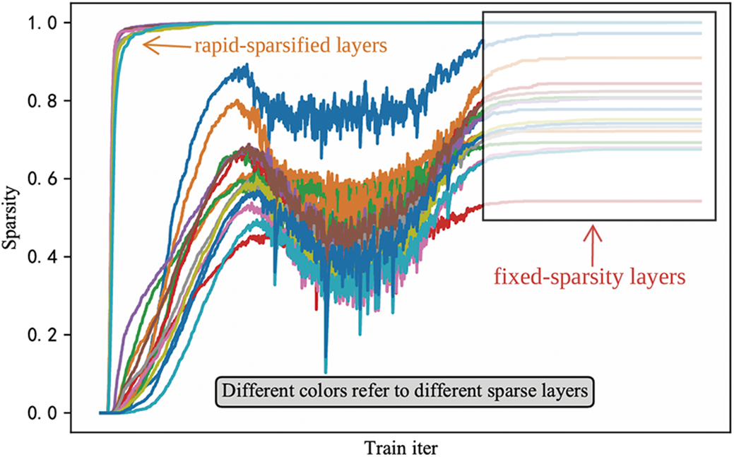
Figure 4: Sparsity variation of all SECOND layers during training process with SWP (Stripe-Wise Pruning)

3.3 Hierarchical Shape Pruning

This section describes how to update pruning thresholds hierarchically based on SWP. As with SWP, to make the distribution of FS sparse enough during training, i.e., to keep some elements of FS below a threshold, sparse regularization needs to be applied to FS during training, corresponding to a model loss function of:

ℒ=∑(x,y)loss(f(x,W⊙F),y)+λg(F)(3)

where (x,y) is the training data, W is the model parameter, ⊙ denotes the dot product operation, λ stands for the magnitude of sparse regularization, F stands for FS, and g(F) denotes the sparse regularization applied to FS using the ℓ1-norm:

g(F)=∑l=1Lg(Fl)=∑l=1L(∑i=1N∑j=1K∑k=1K|Fi,j,kl|)(4)

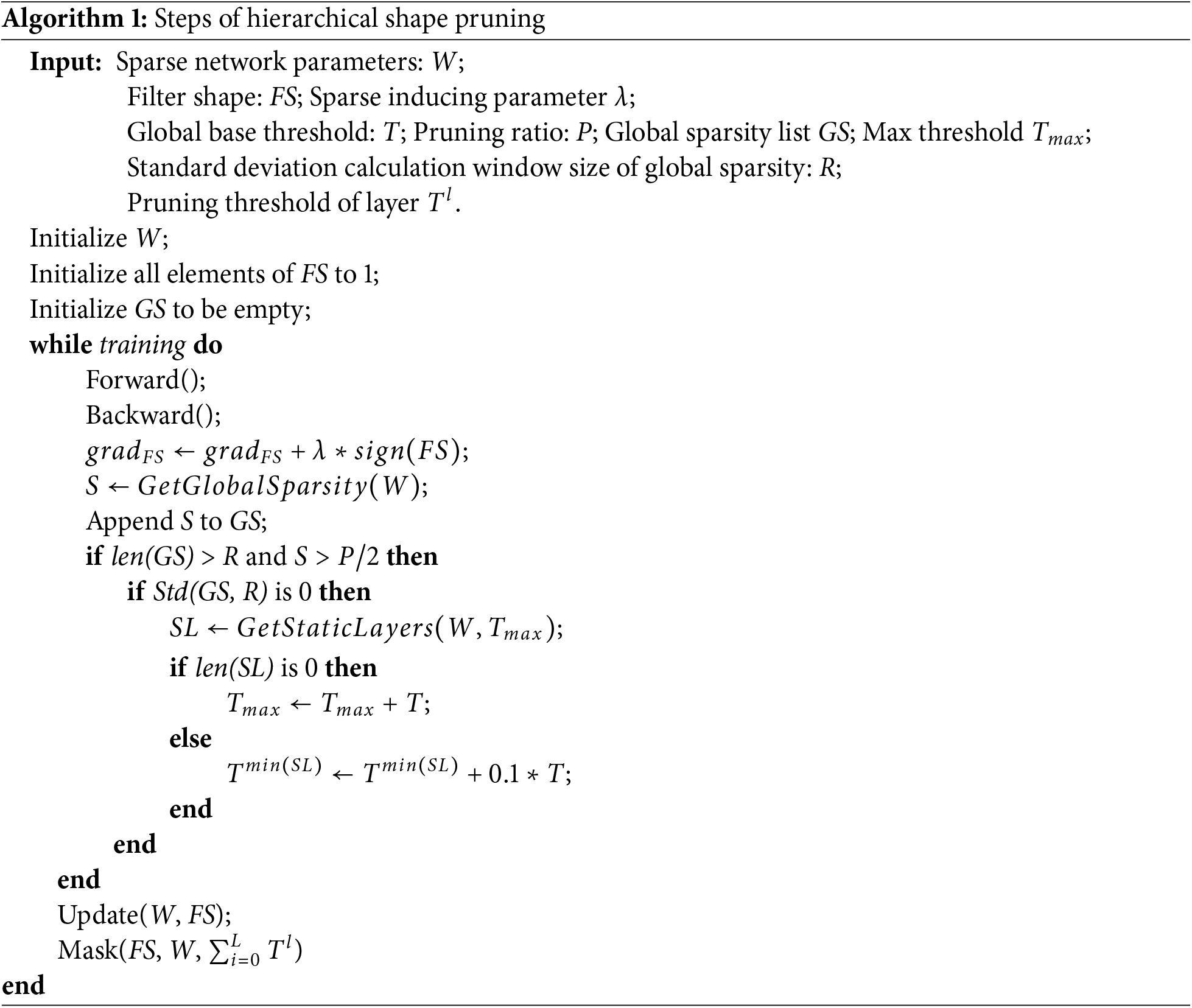
Next, we describe in detail how to set dynamic thresholds in different sparse convolutional layers. First, we define a global threshold T as the basis for the dynamic change of the threshold in each layer, and given a pruning ratio P. During training, the global sparsity S of the network is recorded after each iteration, and the standard deviation of the historical global sparsity within a certain window is counted when S is larger than P/2:

Std(GS,R)=1R∑r=1R(GSr−μ)2(5)

where GS denotes all the global sparsity from the beginning of training to the current iteration, R denotes the number of historical global sparsity counted forward from the current iteration, i.e., the size of the standard deviation statistical window, GSr denotes all historical global sparsity within the window, and μ is the mean value of historical global sparsity.

When the standard deviation of global sparsity within the monitoring window reaches zero, it indicates that the model’s optimization space—the set of potentially recoverable yet currently pruned stripes—has stagnated. This stagnation implies that the current threshold configuration can no longer explore better sparsity patterns without intervention. To reinvigorate the search, we:

1.    Identify Candidate Layers: Iterate through all layers, flagging those whose sparsity trends align with the global plateau (i.e., zero deviation) and fall within the transition zone [P/2,P].

2.    Thresholds Adjustment: Select the flagged layer with minimal sparsity (mostly under-pruned) and increment its threshold by 0.1T, where T is the base threshold. This targeted increase forces exploration of sparser configurations while preserving critical features in stable layers.

3.    Dynamic Thresholds Ceiling: If all flagged layers reach Tmax, we expand the search space by setting Tmax←Tmax+T, preventing premature convergence to suboptimal sparsity.

This mechanism ensures continuous optimization space exploration when conventional gradient-based updates plateau. See Algorithm 1 for details.

3.4 Compute the Input and Output Indices of an Irregular Convolutional Kernel

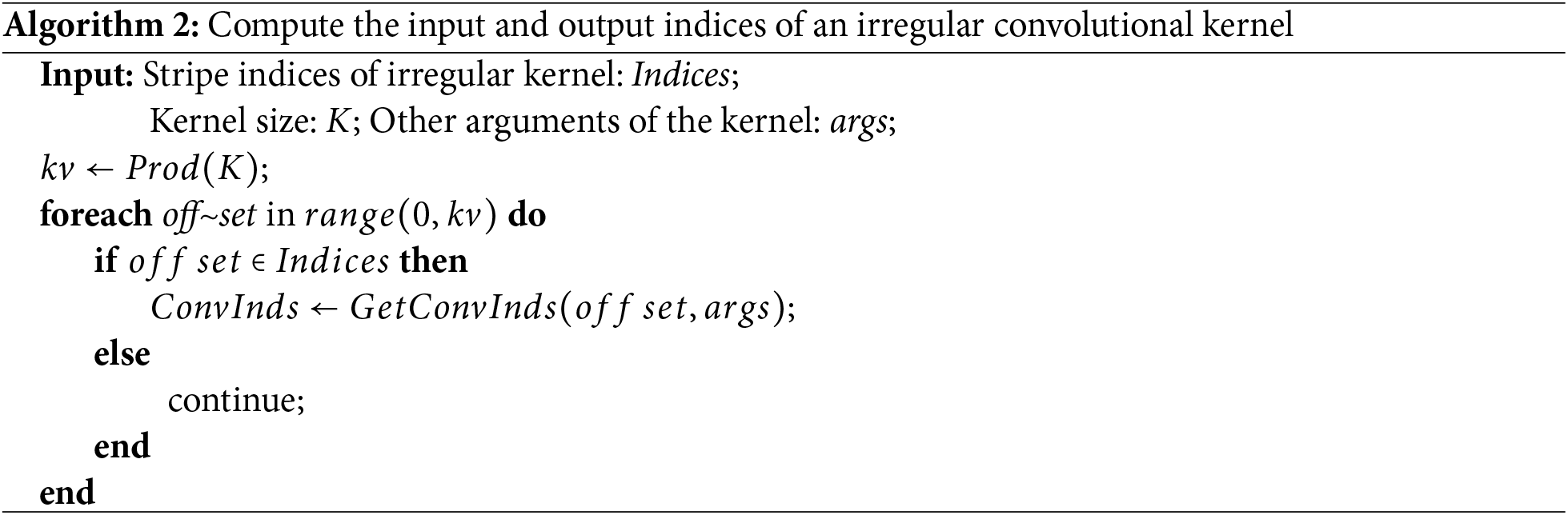
To achieve the convolution of irregular kernels generated after shape pruning, SWP splits the irregular kernel into many individual stripes, i.e., these 1D convolutions are used to accumulate the outputs after sliding them over the input data.

However, for sparse convolution, all that is needed in the forward derivation is to determine whether the convolution kernel stripes is legal or not when traversing the convolution kernel to obtain the index of the convolution output. While storing the parameters of the irregular sparse convolution kernel, the same irregular sparse convolution kernel is also split into a separate stripe, the difference is that the index attribute is attached to it, which is used to determine whether the index is legal or not in the forward derivation.

Based on the irregular convolution kernel, the detail of computing the input and output indices is shown in Algorithm 2. While for the submanifold 3D sparse convolution, if the center stripe of the convolution kernel is set to zero during the pruning process, zero is still considered to be a valid value because the submanifold 3D sparse convolution needs to use the center of the kernel to determine whether output indexing is needed. For details about the output index calculation of sparse convolution, refer to the sparse convolution library SPConv1.

4  Experiments

This section begins with an introduction to the experimental setup. Then we compare HSP-S with SWP on voxel-based 3D object detection models using sparse convolution, to highlight the superiority of the proposed HSP-S pruning method. Furthermore, to deeply explore the performance of the HSP-S pruning method, we perform experimental comparisons on 2D classification model ResNet56 [21]. Finally, we perform ablation experiments to explore the effect of hyperparameters in HSP-S on its pruning performance.

4.1 Setup

Datasets. In our experiments, we use the KITTI dataset and NuScenes dataset, which are commonly used in 3D object detection models. The KITTI dataset contains 7481 training samples and 7518 test samples. Since the test samples are not visible, we divide the 7481 training samples into two subsets the training set and the test set, with sample numbers of 3712 and 3769, respectively. Each sample scene consists of lidar data and the corresponding image data, and only the three categories of Pedestrian, Car, and Cyclist are considered in it. NuScenes dataset contains 1000 samples, of which the number of samples in the training, validation, and test sets are 700, 150, and 150, respectively. Each sample scene consists of lidar data and multi-view image data and contains 10 categories. In this paper, the 2D classification dataset used in the experiments is CIFAR10, which contains 10 categories, the training set contains 50,000 images, and the test set contains 10,000 images.

Models. Our experiments are conducted based on MMDetection3d [26] toolbox and select the voxel-based 3D object detection models as the target models to be pruned. For the KITTI dataset, the target models include SECOND [2], PartA2 [5], PV-RCNN [6], MVXNet [27]; for the NuScenes dataset, we only test CenterPoint [28], cause is the only outdoor 3D object detection model based on voxels. Due to the complex structure of the 3D object detection models, the voxel feature extraction backbone is the target component for pruning. As for the CIFAR10 dataset, the target model is ResNet56, which is always used to be pruned by existing pruning methods.

Baseline. For 3D object detection models based on the KITTI dataset, we train 40 epochs, and for CenterPoint, we train 20 epochs. And for ResNet56, we train 160 epochs. The parameters other than the number of training epochs, such as the learning rate, data enhancement strategy, and batch size, we just follow the original configuration of each model.

Pruning Settings. Since SWP has not been tested on voxel-based 3D object detection models, for comparison purposes, experiments are conducted on the above 3D object detection models using SWP. For SWP, the hyperparameter λ in Eq. (3) is set to 1e−5, the global threshold T is set to 0.01, and no retraining is performed after pruning. For HSP-S, the hyperparameter λ and global threshold T is the same as for SWP, the pruning rate is set to 0.95, the sparsity standard deviation statistical window size R is set to 2 epochs, and the maximum threshold Tmax is set to 0.03.

Pruning Performance. We conduct pruning on the the voxel feature extraction backbone of 3D object detection models, so the rest of the model also contains learnable parameters, making traditional pruning performance metrics of the number of parameters (Params) and the amount of computation (FLOPs, Floating Point Operations per Second) not accurately reflect the pruning effect. So we use the global sparsity S (i.e., the proportion of the number of Params decreasing) and the loss of the model’s accuracy of the voxel feature extraction backbone network as metrics to measure the performance of pruning methods.

4.2 Results on Voxel-Based 3D Object Detection Models

This section compares the pruning performance of HSP-S and SWP on various voxel-based 3D object detection models (see Table 1).

KITTI. On the KITTI dataset, HSP-S achieves higher sparsity than SWP on PartA2, PV-RCNN and MVXNet and lower sparsity on Second. As for accuracy after pruning, HSP-S achieves higher accuracy on the 4 models above.

NuScenes. On the NuScenes dataset, HSP-S achieves both higher sparsity and better accuracy than SWP.

Based on the above results, the model sparsity after HSP-S pruning is higher than that of SWP except for SECOND, and even though the sparsity after HSP-S pruning is lower than that of SWP for SECOND, the two values are very close to each other and are almost negligible. As for the model accuracy after pruning, it can be seen that HSP-S achieves even higher accuracy than the baseline model on both SECOND and CenterPoint, and both are substantially better than the model accuracy after SWP pruning. For example, for CenterPoint, the model accuracy (mAP and NDS) is improved by 1.02%/0.47% after pruning with HSP-S, while the model accuracy is decreased by 0.04%/0.17% after pruning with SWP, which shows a very obvious advantage of HSP-S. For other models, the model accuracy after HSP-S pruning is also completely higher than that after SWP pruning. In addition, both SWP and HSP-S could only achieve about 20% sparsity, which suggests that setting 0.01 as the global threshold for SWP and the base threshold for HSP-S should be smaller. Actually, this empirically driven base global threshold reveals a limitation: the need for manual tuning introduces subjectivity and compromises reproducibility across tasks.

By adjusting the pruning thresholds at different layers of the network, HSP-S can further expand the pruning ratio of the model to be closer to the predetermined pruning ratio, and in the process of adjusting the thresholds, the potential of the soft pruning method is explored, and the shape of filters is continually changed during the training, which further enlarges the optimization space of the model parameters.

4.3 Results on ResNet56

To further explore the pruning performance of our pruning method, we conduct experiments on non-sparse convolutional networks, i.e., ResNet56, which is a classification network for recognizing images in the CIFAR10 dataset. Specifically, based on ResNet56, we compare HSP-S with some classical pruning methods and recently proposed excellent pruning methods. The results are shown in Table 2. It can be seen that the model accuracy drop after pruning with HSP-S is 0.08%, while with SWP pruning, the model accuracy drop is 0.12%, HSP-S is more advantageous in terms of the accuracy drop compared with SWP and other methods. At the same time, HSP-S can further reduce the model FLOPs than any other pruning methods.

4.4 Ablation Study

In this subsection, we explore the effect of hyperparameter in HSP-S on its pruning performance. We mainly focus on the hyperparameter R, which controls the frequency of updating thresholds. Table 3 shows the experimental results. We find that R=1238×2 gives the most acceptable sparsity and accuracy.

5  Conclusions

This paper proposes Hierarchical Shape Pruning for 3D Sparse Convolutions (HSP-S), a novel framework that addresses critical inefficiencies in 3D sparse convolutional networks. We first establish that the sparse voxel distributions naturally align with shape-wise pruning, enabling targeted removal of underutilized convolutional stripes while preserving task-critical features. Unlike prior methods relying on static global thresholds, HSP-S introduces layer-specific dynamic adaptation, where gradient-based saliency estimates guide per-layer threshold updates, thus enlarges the optimization space further. To align sparse convolution, HSP processes only non-zero stripes during forward passes of pruned kernels. Extensive experiments on KITTI and NuScenes demonstrate that our method is superior to the existing shape pruning method. A future extension of HSP-S would involve multimodal-guided pruning that fuses camera-based semantic segmentation (e.g., Mask R-CNN(Region-based Convolutional Neural Networks) outputs) to inform stripe preservation decisions. Specifically, semantic importance maps from 2D images could be projected into 3D voxel space via calibration matrices, creating soft constraints that protect convolution stripes overlapping with high-value semantic regions.

Acknowledgement: We would like to thank the contributors of the open-source project MMDetection3D.

Funding Statement: The authors received no specific funding for this study.

Author Contributions: The authors confirm contribution to the paper as follows: Conceptualization: Haiyan Long and Chonghao Zhang; methodology: Chonghao Zhang and Hai Chen; software: Chonghao Zhang; validation: Haiyan Long, Chonghao Zhang and Gang Chen; formal analysis: Hai Chen; investigation: Chonghao Zhang; resources: Chonghao Zhang and Hai Chen; data curation: Chonghao Zhang; writing—original draft preparation: Chonghao Zhang; writing—review and editing: Haiyan Long, Xudong Qiu and Gang Chen; visualization: Chonghao Zhang; supervision: Hai Chen; project administration: Haiyan Long. All authors reviewed the results and approved the final version of the manuscript.

Availability of Data and Materials: The data that support the findings of this study are openly available at https://www.cvlibs.net/datasets/kitti/ (accessed on 15 April 2024) and https://www.nuscenes.org/ (accessed on 15 April 2024).

Ethics Approval: Not applicable.

Conflicts of Interest: The authors declare no conflicts of interest to report regarding the present study.

1https://github.com/traveller59/spconv (accessed on 08 May 2025).

References

1. Graham B, Engelcke M, Van Der Maaten L. 3D semantic segmentation with submanifold sparse convolutional networks. In: Proceedings of the IEEE Conference on Computer Vision and Pattern Recognition. Salt Lake City, UT, USA; 2018. p. 9224–32. [Google Scholar]

2. Yan Y, Mao Y, Li B. Second: sparsely embedded convolutional detection. Sensors. 2018;18(10):3337. doi:10.3390/s18103337. [Google Scholar] [PubMed] [CrossRef]

3. Tang H, Liu Z, Zhao S, Lin Y, Lin J, Wang H, et al. Searching efficient 3D architectures with sparse point-voxel convolution. In: European Conference on Computer Vision. Glasgow, UK: Springer; 2020. p. 685–702. doi:10.1007/978-3-030-58604-1_41. [Google Scholar] [CrossRef]

4. Zhu X, Ma Y, Wang T, Xu Y, Shi J, Lin D. SSN: shape signature networks for multi-class object detection from point clouds. In: Proceedings of the European Conference on Computer Vision. Glasgow, UK: Springer; 2020. p. 581–97. doi:10.1007/978-3-030-58595-2_35. [Google Scholar] [CrossRef]

5. Shi S, Wang Z, Shi J, Wang X, Li H. From points to parts: 3D object detection from point cloud with part-aware and part-aggregation network. IEEE Trans Pattern Anal Mach Intell. 2020. doi:10.1109/tpami.2020.2977026. [Google Scholar] [PubMed] [CrossRef]

6. Shi S, Guo C, Jiang L, Wang Z, Shi J, Wang X, et al. PV-RCNN: point-voxel feature set abstraction for 3D object detection. In: Proceedings of the IEEE/CVF Conference on Computer Vision and Pattern Recognition (CVPR); 2020. p. 10529–38. [Google Scholar]

7. Meng F, Cheng H, Li K, Luo H, Guo X, Lu G, et al. Pruning filter in filter. Adv Neural Inf Process Syst. 2020;33:17629–40. [Google Scholar]

8. He Y, Kang G, Dong X, Fu Y, Yang Y. Soft filter pruning for accelerating deep convolutional neural networks. arXiv:1808.06866. 2018. [Google Scholar]

9. Li H, Kadav A, Durdanovic I, Samet H, Graf HP. Pruning filters for efficient convnets. arXiv:1608.08710. 2016. [Google Scholar]

10. Jiang P, Xue Y, Neri F. Convolutional neural network pruning based on multi-objective feature map selection for image classification. Appl Soft Comput. 2023;139(1):110229. doi:10.1016/j.asoc.2023.110229. [Google Scholar] [CrossRef]

11. Hinton G, Vinyals O, Dean J. Distilling the knowledge in a neural network. arXiv:1503.02531. 2015. [Google Scholar]

12. Li J, Zhao R, Huang JT, Gong Y. Learning small-size DNN with output-distribution-based criteria. In: Interspeech 2014. Singapore; 2014. p. 1910–4. [Google Scholar]

13. Nagel M, Baalen MV, Blankevoort T, Welling M. Data-free quantization through weight equalization and bias correction. In: Proceedings of the IEEE/CVF International Conference on Computer Vision; 2019; Seoul, Republic of Korea. p. 1325–34. [Google Scholar]

14. Banner R, Nahshan Y, Soudry D. Post training 4-bit quantization of convolutional networks for rapid-deployment. Vol. 32. In: Advances in neural information processing systems. Vancouver, BC, Canada: Curran Associates, Inc.; 2019. [Google Scholar]

15. Xue Y, Chen C, Słowik A. Neural architecture search based on a multi-objective evolutionary algorithm with probability stack. IEEE Trans Evol Comput. 2023;27(4):778–86. doi:10.1109/tevc.2023.3252612. [Google Scholar] [CrossRef]

16. Han S, Mao H, Dally WJ. Deep compression: compressing deep neural networks with pruning, trained quantization and huffman coding. arXiv:1510.00149. 2015. [Google Scholar]

17. Hu H, Peng R, Tai YW, Tang CK. Network trimming: a data-driven neuron pruning approach towards efficient deep architectures. arXiv:1607.03250. 2016. [Google Scholar]

18. Luo JH, Wu J, Lin W. Thinet: a filter level pruning method for deep neural network compression. In: Proceedings of the IEEE International Conference on Computer Vision. Venice, Italy; 2017. p. 5058–66. [Google Scholar]

19. Molchanov P, Tyree S, Karras T, Aila T, Kautz J. Pruning convolutional neural networks for resource efficient inference. arXiv:1611.06440. 2016. [Google Scholar]

20. Liu Z, Li J, Shen Z, Huang G, Yan S, Zhang C. Learning efficient convolutional networks through network slimming. In: Proceedings of the IEEE International Conference on Computer Vision. Venice, Italy; 2017. p. 2736–44. [Google Scholar]

21. He K, Zhang X, Ren S, Sun J. Deep residual learning for image recognition. In: Proceedings of the IEEE Conference on Computer Vision and Pattern Recognition. Las Vegas, NV, USA; 2016. p. 770–8. [Google Scholar]

22. Yu R, Li A, Chen CF, Lai JH, Morariu VI, Han X, et al. Nisp: pruning networks using neuron importance score propagation. In: Proceedings of the IEEE Conference on Computer Vision and Pattern Recognition. Salt Lake City, UT, USA; 2018. p. 9194–203. [Google Scholar]

23. Zhuang Z, Tan M, Zhuang B, Liu J, Guo Y, Wu Q, et al. Discrimination-aware channel pruning for deep neural networks. In: Advances in neural information processing systems. Vol. 31; 2018. [Google Scholar]

24. You Z, Yan K, Ye J, Ma M, Wang P. Gate decorator: global filter pruning method for accelerating deep convolutional neural networks. In: Advances in neural information processing systems. Red Hook, NY, USA: Curran Associates Inc.; 2019. [Google Scholar]

25. Lin M, Ji R, Wang Y, Zhang Y, Zhang B, Tian Y, et al. HRank: Filter pruning using high-rank feature map. In: Proceedings of the IEEE/CVF Conference on Computer Vision and Pattern Recognition. Seattle, USA; 2020. p. 1529–38. [Google Scholar]

26. Contributors M. MMDetection3D: openMMLab next-generation platform for general 3D object detection; 2020 [cited 2025 Apr 7]. Available from: https://github.com/open-mmlab/mmdetection3d. [Google Scholar]

27. Sindagi VA, Zhou Y, Tuzel O. MVX-Net: multimodal voxelnet for 3D object detection. In: 2019 International Conference on Robotics and Automation (ICRA). Montreal, QC, Canada; 2019. p. 7276–82. doi:10.1109/ICRA.2019.8794195. [Google Scholar] [CrossRef]

28. Yin T, Zhou X, Krähenbühl P. Center-based 3D object detection and tracking. In: Proceedings of the IEEE/CVF Conference on Computer Vision and Pattern Recognition (CVPR); 2021. p. 11784–93. [Google Scholar]