Pathfinder: Deep Reinforcement Learning-Based Scheduling for Multi-Robot Systems in Smart Factories with Mass Customization

1  Introduction

As the Fourth Industrial Revolution progresses and Industry 4.0 evolves, artificial intelligence (AI) emerges as a pivotal force in diverse sectors [1]. The advent and progression of robotics technology have enabled the replacement of numerous conventional manual tasks, showcasing broad potential across various domains. Robots find applications from factory production to healthcare, and from logistics to household services, indicating their extensive future potential [2]. For instance, industrial robots significantly enhance efficiency and quality on automated assembly lines [3], while medical robots achieve precision in surgeries and diagnostics [4]. Additionally, smart home robots offer essential daily services. These advancements not only improve productivity but also ensure precision and reliability in complex tasks, gaining extensive recognition and significant interest from both academia and industry.

In contemporary society, smart factories epitomize the essence of Industry 4.0. These facilities incorporate cutting-edge technologies like Cyber-Physical Systems (CPS) [5], the Internet of Things (IoT) [6], big data [7], multi-robot systems [8], and virtual reality [9], enabling automation, digitization, and intelligence in manufacturing processes [10]. Distinguished from traditional manufacturing setups, smart factories offer enhanced flexibility and efficiency. They support real-time monitoring, predictive maintenance, and autonomous process optimization. These capabilities not only boost production efficiency and reduce operational costs but also allow swift adaptation to market changes, securing a competitive advantage for businesses [11].

In the realm of smart factories, industrial robots are indispensable, enhancing production and material transport efficiencies significantly. These include robotic arms and autonomous mobile robots, which not only reduce labor costs but also redirect human resources towards activities of higher value [12]. Extensive research within both academia and industry has yielded innovative solutions for intelligent production. These encompass areas such as production scheduling [13], resource allocation [14], logistics, storage [15], and emergency management [16].

Traditional industrial production processes are rigid, with flexibility constrained by the limited number of dedicated production lines. In contrast, dynamic customized production in smart factories demands production lines capable of handling mixed and multi-batch dynamic tasks [17]. The shift towards intelligent manufacturing emphasizes reconfigurable, multi-use dynamic production that can adapt in real-time to produce various products by leveraging AI, robotics, sensors, and information communication technology. However, this approach presents scheduling challenges, including time-varying machine structures, varying processing speeds of parallel machines, and dynamic job arrivals.

In traditional industrial production scheduling, practitioners typically rely on manually selecting one or more fixed scheduling rules based on past experience [18], requiring significant expertise. However, with the increasing complexity and flexibility demanded by customized production and unexpected events, the efficiency and robustness of scheduling cannot always be assured. Moreover, existing scheduling methods often prioritize local optimization, lacking a global perspective, which results in reduced production efficiency and resource utilization.

To address these challenges, Pathfinder, a scheduling approach, was developed by integrating deep learning and reinforcement learning, enabling autonomous adaptation and optimization of scheduling strategies in real-time production environments. Pathfinder efficiently manages uncertainties and dynamic fluctuations, achieving global optimization to maximize production efficiency. Experimental results demonstrate Pathfinder’s superior performance on various classic scheduling datasets, offering insights and methodologies for advancing smart factory operations.

The main contributions include:

•   A specialized reward function is designed to support dynamic task allocation and real-time adjustments, creating a novel multi-robot job scheduling model tailored for smart factories. This approach improves production efficiency and optimizes robot coordination.

•   An adaptable approach was adopted by selecting ten diverse scheduling rules instead of fixed actions. These rules enhance decision-making flexibility, with the optimal rule dynamically chosen based on environmental conditions. This strategy addresses the challenge of reflecting changes in custom production scheduling, allowing the model to adapt to dynamic scenarios and maintain optimal performance.

•   A method called Pathfinder is proposed for decision-making in custom production job scheduling. It transforms scheduling data into matrices of execution time, completion time, and efficiency. By utilizing neural networks to extract features, Pathfinder optimizes machine utilization and minimizes job completion times, adapting to dynamic production demands and ensuring robust performance in real-world applications.

The paper is structured as follows: Section 2 reviews related work and motivation. Section 3 defines the problem and models. Section 4outlines the approach, followed by implementation in Section 5. Section 6 presents experimental validation, and Section 7 concludes with key contributions.

2  Related Work and Motivation

In this chapter, we present previous researchs on relevant issues and the challenges they have faced. Additionally, we elucidate the motivation behind proposing this algorithm.

2.1 Related Work

Scheduling theory faces significant challenges in task allocation and sequencing within complex systems, particularly in multi-stage scheduling where genetic algorithms and ant colony optimization enhance efficiency [19]. These systems, characterized by their NP-complete or NP-hard nature, necessitate heuristic algorithms for practical solutions.

The evolution of smart factories has introduced complexities that require managing diverse production tasks [20]. Innovations in this domain include Wang et al.’s adaptive scheduling using edge computing [21] and Sharif et al.’s optimized resource allocation in health monitoring [22].

Edge computing’s pivotal role in intelligent manufacturing supports real-time applications such as augmented reality [23] and resource-efficient scheduling algorithms like the Whale Optimization algorithm [24].

In collaborative robotics, efficient task allocation and multi-robot cooperation strategies are explored by Baroudi et al., Dutta et al., and Wei et al. [25–27]. Quantum reinforcement learning for enhanced control is also being investigated in smart factories [28].

Deep reinforcement learning (DRL) has been applied to dynamic scheduling, with models like Zhang et al.’s DeepMAG integrating multi-agent systems for better decision-making [29]. Similar strategies were explored by Han et al. and Zhou et al. to enhance production in smart factories [30,31]. Ma et al. introduced a reliability-aware DRL approach for DNN tasks in mobile-edge computing [32]. Zhang et al. developed a multi-agent manufacturing system using an improved contract network protocol and PPO-trained AI scheduler, showing strong performance under disruptions [33]. Liu et al. proposed a hierarchical, distributed architecture for dynamic job-shop scheduling using a Double Deep Q-Network with tailored state-action spaces and reward shaping for efficient learning [34]. Alexopoulos et al. designed a DRL framework where an agent selects dispatching rules, improving scheduling and makespan in a bicycle production case [35]. Gui et al. employed a composite action framework with a DDPG-trained policy network for job-shop scheduling, outperforming traditional rules and DQN-based methods [36]. Li et al. applied DRL with PPO and a recurrent neural network to parallel machine scheduling with family setup constraints, achieving strong generalization and superior performance over heuristics [37].

2.2 Motivation

Traditional fixed production lines with multiple robots face challenges in adapting to the flexibility needed for customized manufacturing. Existing methods lack the ability to reconfigure multi-robot tasks or adjust to dynamic schedules, limiting flexible production management.

Maximizing net profit requires considering resource consumption, robot types, energy use, and load balancing. Use of robot resources, including completion time and utilization rate, is vital.

We propose a reinforcement learning-based approach to optimize multi-robot task configurations in complex environments, enhanced by deep learning for high-dimensional data processing. This improves accuracy, efficiency, and flexibility through universal scheduling rules. Immediate rewards are tied to scheduling efficiency and utilization rates for precise goal evaluation.

By modeling the scheduling problem as a Markov decision process and applying a Deep Q Network, our method enables intelligent, collaborative, and adaptive robot scheduling in smart factories, ensuring robust performance under dynamic conditions.

3  Problem Description and Formulation

In this chapter, we introduce the problem and provide a formal description of it. Then, we proceed to establish the corresponding mathematical model.

3.1 Preliminaries

Reinforcement learning is used to learn action-selection strategies by modeling the scheduling problem as a Markov Decision Process (MDP). An MDP assumes that future states and rewards depend solely on the current state and action, not on past states. Thus, the problem must be framed accordingly. A standard MDP is defined by a quintuple:

MDP=<S,A,Pss′a,Rss′a,γ>(1)

In this paper, the state space S={s1,s2,. . .,sT} represents all possible environmental configurations, where each state includes matrices for execution time, completion time, and task efficiency per robot. The action space A={a1,a2,. . .,aT} consists of ten common scheduling rules.

The transition probability Pss′a defines the likelihood of reaching state s′ from s via action a, reflecting varied outcomes from applying a rule:

Pss′a=1number of reachable states(2)

The immediate reward function Rss′a quantifies the reward for such transitions, and the discount factor γ balances short-term and long-term gains.

Training begins by estimating the action-value function Q(s,a), the expected return from taking action a in state s. The optimal value Q∗(s,a) satisfies the Bellman equation and determines the best action to maximize expected reward:

Q∗(s,a)=E[rt+1+γmaxa′Q∗(st+1,at+1)|st=s,at=a](3)

Then, update the action value function by updating the Q-values. The update formula for Q-values is as follows:

Q(s,a)←Q(s,a)+α[r+γmaxaQ(s′,a′)−Q(s,a)](4)

here, α is the learning rate, controlling the extent to which new rewards affect the Q-values. The action-value function is stored in the Q-table. This iteration process continues until the task is completed, and the cumulative reward Rt=∑t′Tγt′−trt reflects the total reward obtained by the agent before the interaction ends. The entire process is illustrated in the Fig. 1.

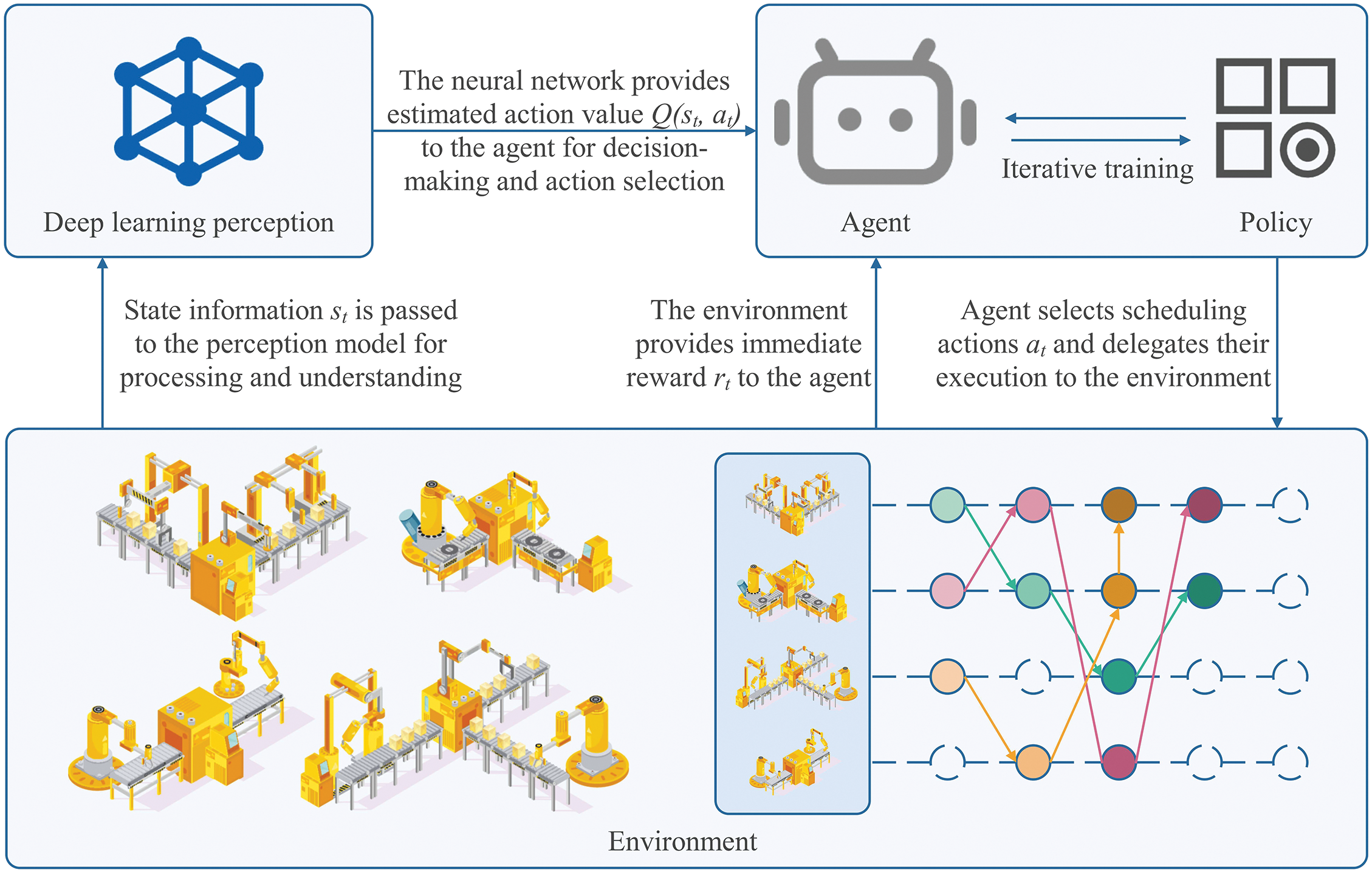
Figure 1: Deep reinforcement learning scheduling model

3.2 Problem Description

In this scheduling problem, we have a manufacturing system with a set of orders O={Oi,i=1,2,…,N}. Each order Oi comprises a sequence of jobs Ji={Jij,j=1,2,…,NJi}, where NJ={NJi,i=1,2,…,N} represents the total number of jobs for each order. These jobs must be executed in a predefined order. Additionally, the system is equipped with a set of robots R={Rm,m=1,2,…,M}, and each job is assigned to a specific robot. The constraint relationship set E={Eijm,i=1,2,…,N,j=1,2,…,NJi,m=1,2,…,M} defines which robot can execute each job.

For robots to be effective in completing orders, a description is shown as follows:

Input: Set of orders O={Oi,i=1,2,…,N}. Jobs for each order Ji={Jij,j=1,2,…,NJi}. Total number of jobs for each order NJ={NJi,i=1,2,…,N}. Set of robots R={Rm,m=1,2,…,M}. Constraint relationship set E={Eijm,i=1,2,…,N,j=1,2,…,NJi,m=1,2,…,M}. Execution time of orders P={Pi,i=1,2,…,N}, where Pi represents the actual time required to execute order Oi, meaning the total time spent actively processing the order. This does not include any waiting time before execution starts. Execution time of jobs PJ={PJij,i=1,2,…,N,j=1,2,…,NJi}.

Output: Completion time of orders C={Ci,i=1,2,…,N}, where Ci represents the time when order Oi is fully processed and considered completed. It includes both the waiting time before execution begins and the execution time itself. Completion time of jobs CJ={CJij,i=1,2,…,N,j=1,2,…,NJi}.

Objective: Maximize U¯, the average utilization of manufacturing robots, by completing orders and tasks in the minimum time. Representing each robot’s utilization as U={Um,m=1,2,…,M}, the optimal scheduling solution requires careful consideration of job sequences and robot availability.

3.3 Mathematical Model

In a smart factory, the job scheduling phase is critical to ensure that the manufacturing resources of each robot are fully utilized. This utilization is primarily reflected in the production duration (makespan) and the average machine utilization (U¯). Below are the specific formulas for calculating these metrics:

makespan=maxiCi(5)

where makespan represents the maximum completion time among all jobs, which serves as the production cycle in job scheduling. Minimizing the makespan is closely tied to maximizing the utilization of robot resources, as reducing the completion time allows for more efficient resource use.

Eq. (6) provides the formula for average machine utilization U¯:

U¯=1M∑m=1M∑i=1N∑j=1NJiPJijmaxiCi=∑i=1NPiM⋅makespan(6)

where M is the number of robots and ∑i=1NPi represents the total processing time of all jobs.

When ∑i=1NPi and M are constants, minimizing the makespan is equivalent to maximizing machine utilization. Thus, the objective is to minimize the makespan:

Minimize makespan=maxiCi=maxiCJi(NJi)(7)

This objective is subject to the following constraints:

1. Job Assignment Constraint: Each job is assigned to at most one robot:

∑m=1MXijm≤1,   i=1,2,…,N,   j=1,2,…,NJi(8)

where Xijm is a binary variable indicating whether job Jij is assigned to robot Rm.

2. Job Sequence Constraint: Jobs must be completed in the specified order:

CJi(j−1)+PJij≤CJij,   i=1,2,…,N,   j=2,…,NJi(9)

3. Completion Time Constraint: The completion time of each job must not exceed the maximum completion time of its associated job sequence:

CJij≤Ci,   i=1,2,…,N,   j=1,2,…,NJi(10)

4. Robot Occupancy Constraint: At any given time, a robot can only be assigned to one job:

∑i=1N∑j=1NJiAijm≤1,   i=1,2,…,N,   j=1,2,…,NJi(11)

where Aijm is a binary variable indicating whether robot Rm is active during Jij (1 if active, 0 otherwise).

5. Robot Availability Constraint: A robot can only execute a job if it is available at the given time:

Aijm≤Bm(t),   i=1,2,…,N,   j=1,2,…,NJi,   m=1,2,…,M,    t∈T(12)

where Bm(t) is a binary variable indicating whether robot Rm is available at time t (1 if available, 0 otherwise). This ensures that a job is only assigned to a robot when it is operational and not undergoing maintenance or other constraints.

6. Task-Robot Feasibility Constraint: A specific job Jij can only be assigned to a robot Rm if it is feasible according to the constraint relationship set E:

Xijm≤Eijm,   i=1,2,…,N,   j=1,2,…,NJi,   m=1,2,…,M(13)

These conditions collectively define the optimization problem. The goal is to find the optimal assignment of jobs to robots, minimizing the makespan, and ensuring compliance with the specified constraints.

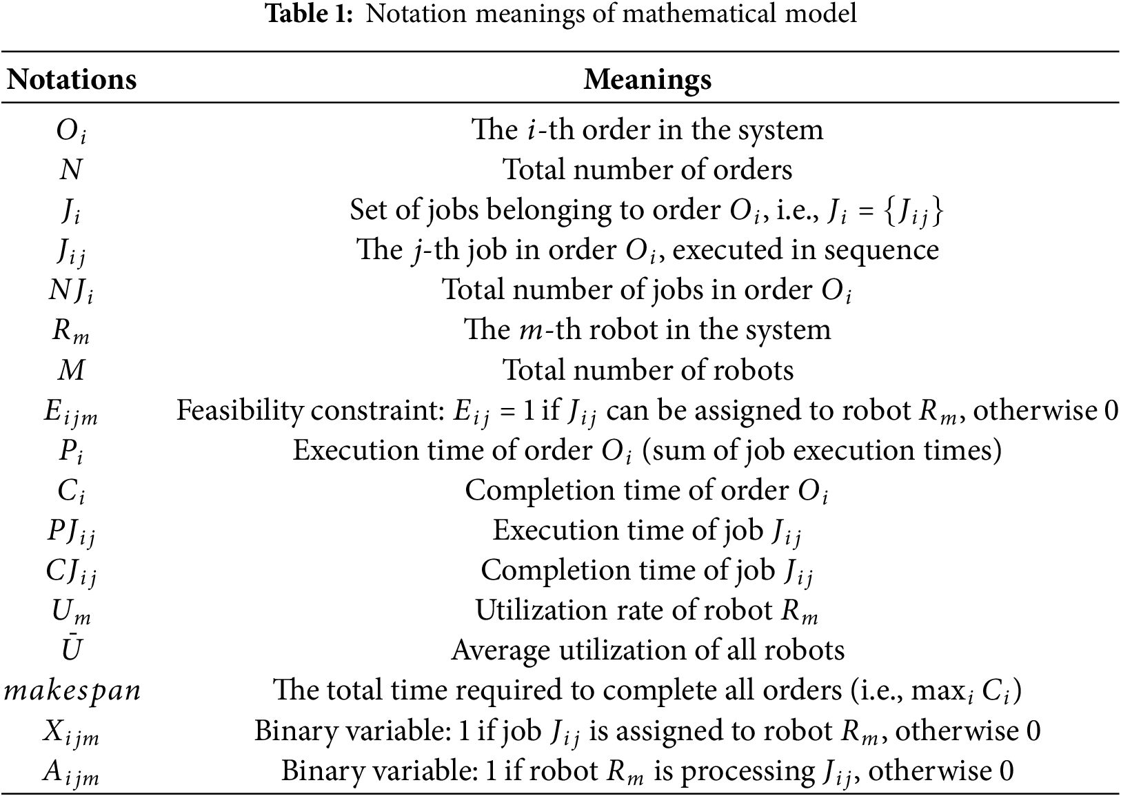
3.4 Table of Mathematical Notations

For improved readability, this paper presents notations and meanings in the Table 1.

4  Proposed Methodology

This chapter offers a thorough overview of the structure of Pathfinder and its complete algorithmic process. Fig. 2 illustrates the overall framework of Pathfinder. Each string of small circles represents an order, where each circle represents a job. The same color indicates that the jobs are executed by the same robot, and the sequence is specified by the arrows. It mainly consists of the following stages.

•   Stage I: Initialization.

Step 1: Establish simulation environment.

–   Step 2: Develop Neural Network.

–   Step 3: Implement experience replay pool.

Stage II: Extracting Experience for NN Training.

–   Step 4: Sample experience data.

–   Step 5: Train the network.

Stage III: Training RL Model for Decisions.

–   Step 6: Interact with virtual environment.

–   Step 7: Update network parameters.

–   Step 8: Store the state sequence (st, a, r, st+1) in the experience replay pool.

Stage IV: Iterative Training and Online Scheduling.

–   Step 9: Repeat training process.

–   Step 10: Enable online job scheduling.

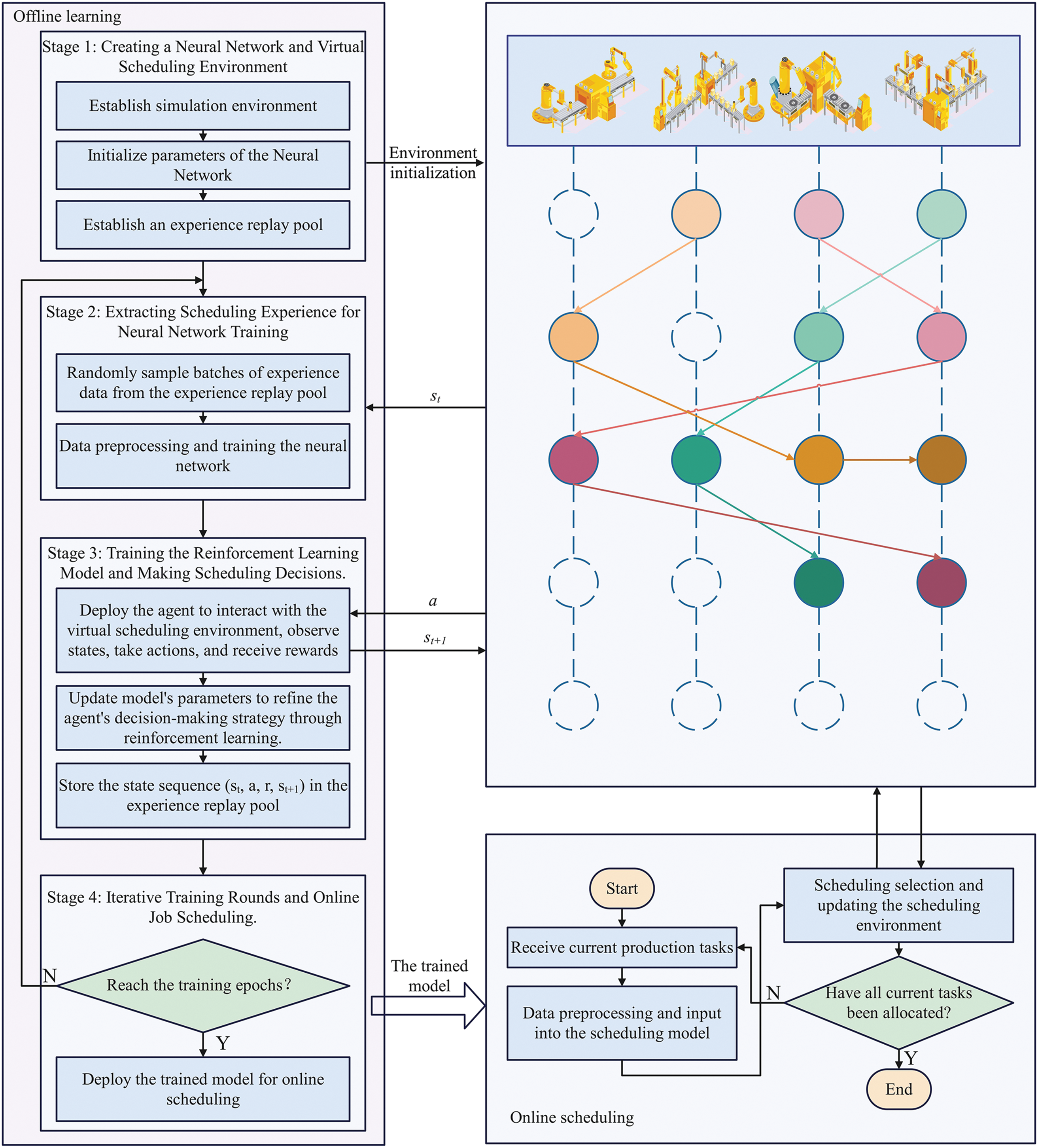
Figure 2: The structure and algorithm flow of Pathfinder

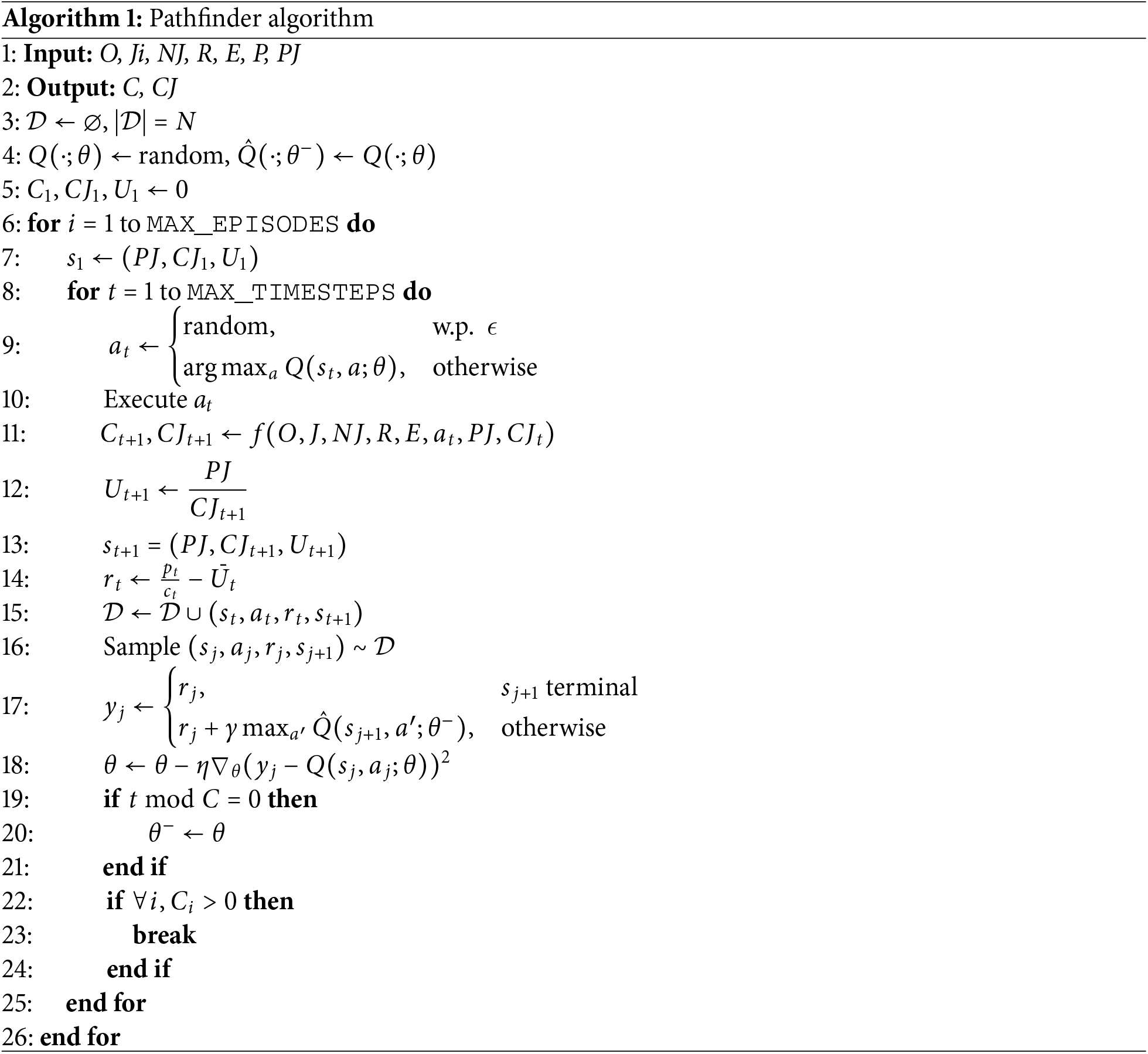
Pathfinder is introduced in Algorithm 1 in detail.

5  Details of Pathfinder

In this chapter, we will delve into the details of each stage in sequential order.

5.1 Establishment of Network Structure and Experience Replay Pool

In the stage 1, our primary focus was on constructing the neural network framework and establishing the experience replay pool. Within this subsection, we’ll delineate the comprehensive structure of both the network and the experience replay pool.

5.1.1 Network Structure

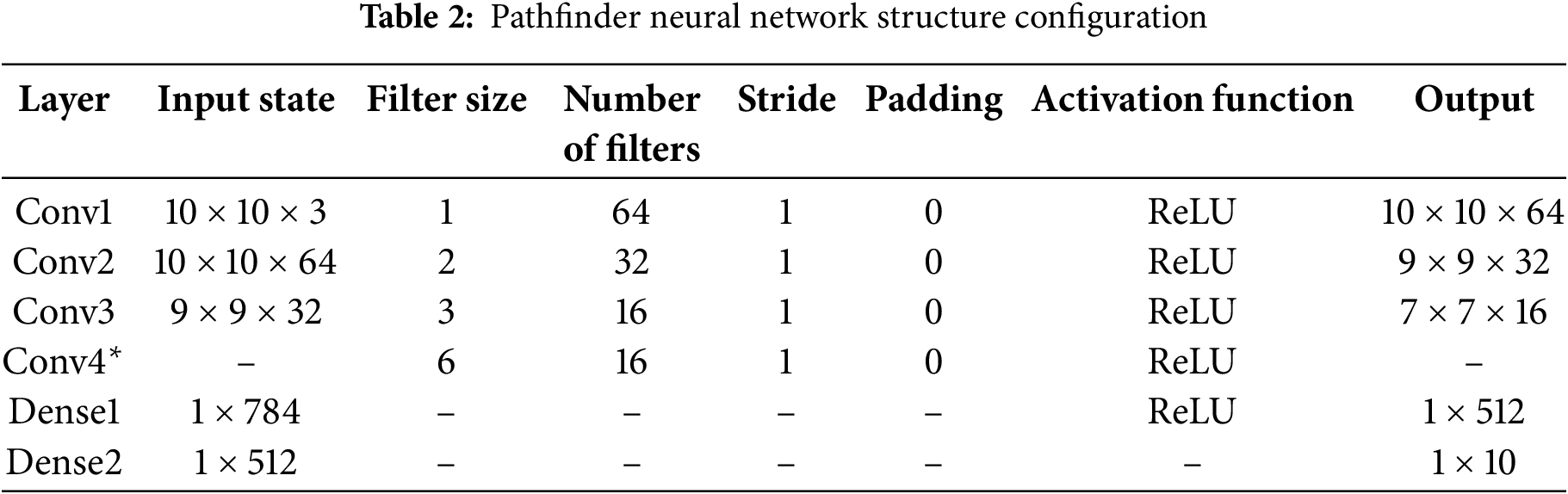
Our scheduling decision model employs a network (Fig. 3) that processes a 3D input matrix of execution time, completion time, and efficiency. The convolutional layer uses square kernels without pooling to preserve feature integrity. We maximize filters in the first layer and reduce them in later layers, keeping the stride fixed at 1. The final convolutional output is flattened and passed to fully connected layers.

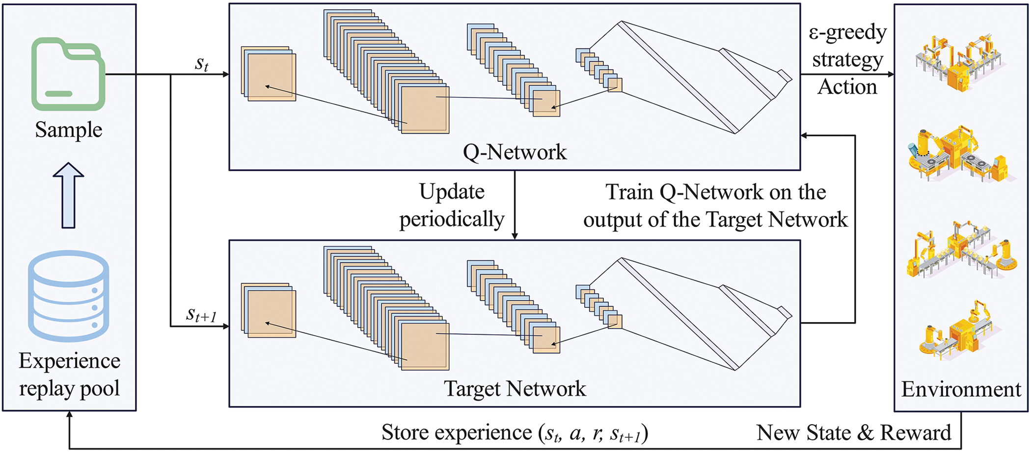
Figure 3: The structure of the Pathfinder scheduling decision model

As detailed in Table 2, the network is configured for a 10 × 10 scheduling dataset. For larger datasets (e.g., over 200 job processes or 20 jobs/orders), a fourth convolutional layer is added to enhance generalization via deeper hierarchical feature extraction.

Our Q-network’s loss function, central to training, is defined as:

L(w)=E[(r+γmaxa′Q(s′,a′,w)−Q(s,a,w))2](14)

Here, L(w) is the loss function measuring the difference between predicted and target Q-values. r is the immediate reward received after transitioning from state s to s′ via action a, with γ as the discount factor for future rewards. a′ is the next action, and w denotes the neural network weights.

With the target Q network, the loss function incorporates target Q-values alongside current Q-values, promoting more stable and effective training:

L(w)=E[(r+γmaxa′Q(s′,a′,w−)−Q(s,a,w))2](15)

where w− represents the weight parameters of the target Q network.

5.1.2 Experience Replay Pool

Pathfinder employs an experience replay pool to improve learning efficiency and stability by reusing past experiences, enhancing sample efficiency and reducing update correlation. Unlike traditional online learning, which updates parameters using only current samples, experience replay enables random sampling from historical data.

This broadens state-action mapping and improves real-time scheduling decisions. As a result, training becomes more efficient, with demonstrated gains in performance and stability.

5.2 State Representation

In stage 2, scheduling data from the experience replay pool is used to train the network. This section explains the state representation in the data.

To address dynamic job scheduling, a three-channel input overlays matrices for machines, job attributes, and scheduling efficiency. For example, in the ft06 dataset (Fig. 4), rows represent orders and column pairs denote jobs–odd columns indicate assigned machines, even columns show execution times. The total number of columns is based on the maximum jobs per order. In the red box example, job 1 of order 1 runs on robot 2 with an execution time of 1.

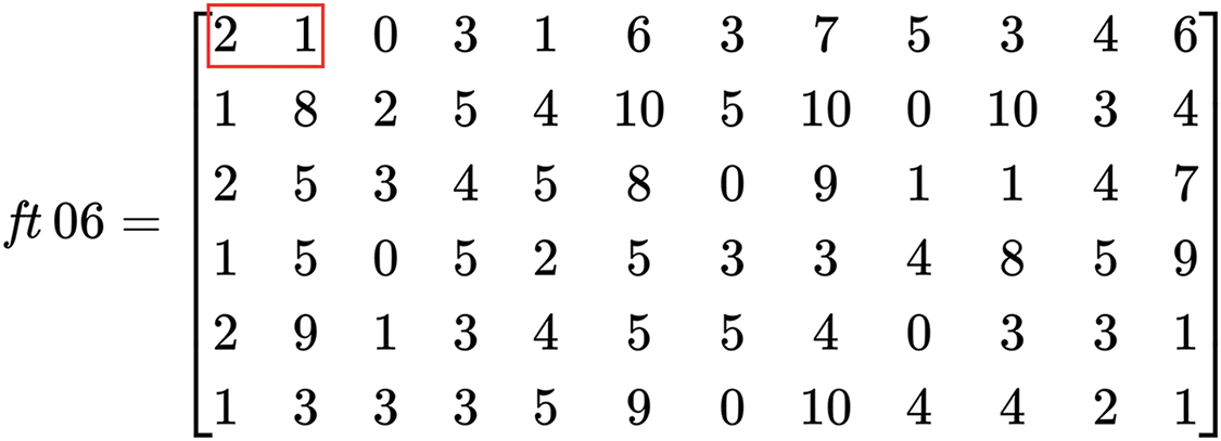
Figure 4: Illustration of the ft06 dataset matrix

The state is formally defined as a tuple of three time-dependent matrices: st=(PJ,CJt,Ut¯). Fig. 5 presents the state matrix after scheduling all jobs for order 1 in the ft06 dataset. The leftmost matrix, PJ, represents the job execution time, where each element PJij denotes the time required to execute job Jij. The central matrix, CJt, corresponds to the completion time at a given time slice t, with each entry CJijt indicating the completion time of job Jij at time t. On the right, the efficiency matrix Ut¯ is computed as the ratio of job execution time to completion time, where Utij¯ quantifies the efficiency of completing the individual job Jij.

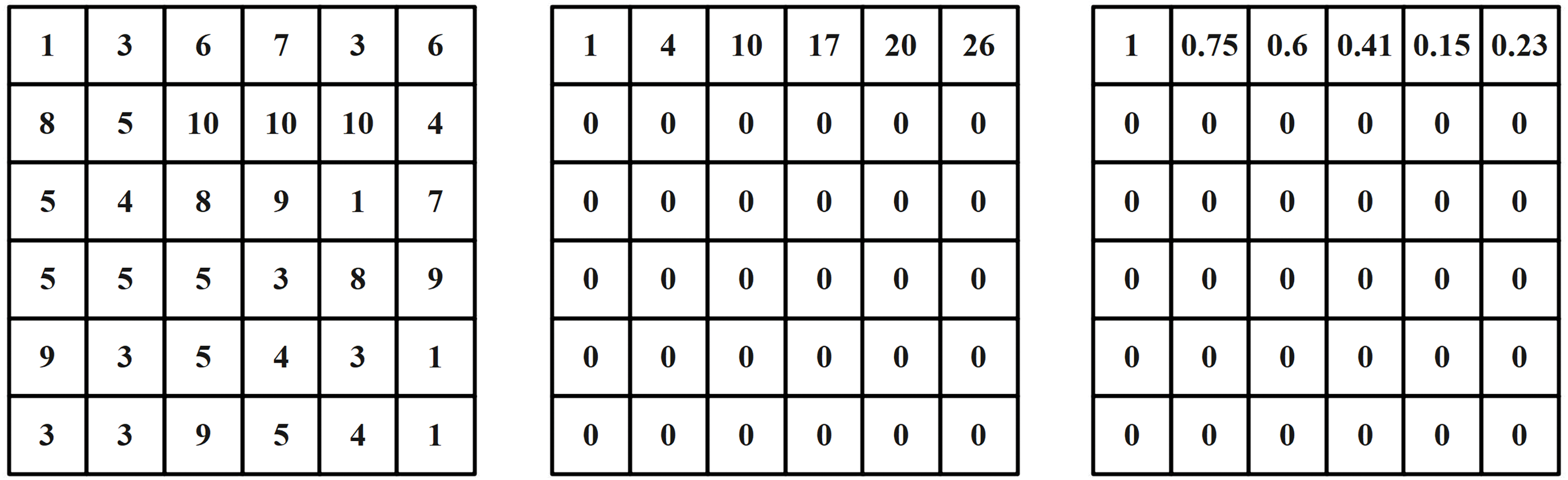
Figure 5: Schedule state matrix for ft06

5.3 Reinforcement Learning Scheduling Algorithm

In stage 3, environmental data is collected to train the reinforcement learning model, guiding algorithm updates and decision-making. This section defines the action space, decision implementation, and reward function.

5.3.1 Action Space

In customized production, scheduling is more complex than in games with clear legal actions due to job dependencies and dynamic production demands. A job may follow different scheduling paths over time, making fixed action outputs insufficient to capture real-world variability.

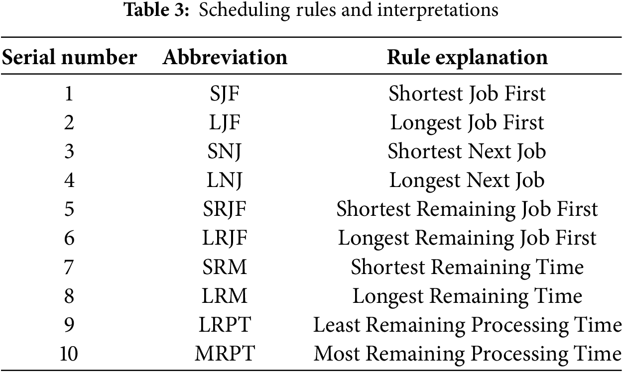
To address this, we adopt general scheduling rules instead of specific actions, improving adaptability to changing conditions. Ten commonly used rules are summarized in Table 3.

5.3.2 Action Decision

In our framework, an action is taken after each job completion, where the agent selects the next scheduling rule.

We use the ε-greedy strategy, which balances exploration and exploitation as follows:

π(a∣s)={1−ε|𝒜(s)|(|𝒜(s)|−1),for the greedy action,ε|𝒜(s)|,for the other |𝒜(s)|−1 actions(16)

here, π(a∣s) denotes the probability of selecting action a in state s, ε∈[0,1] is the exploration rate, and |𝒜(s)| is the number of possible actions. The ε-greedy strategy encourages exploration to discover better scheduling rules, while greedy selection favors the action with the highest Q-value. To ensure convergence, ε decreases over time.

To improve efficiency on large-scale scheduling data, we introduce the cur_policy strategy: when ε<0.2, the model increasingly selects actions with the highest estimated value.

As training progresses, Q-value estimates are continually updated. Unlike traditional Q-learning, deep reinforcement learning approximates Q-values via neural networks. The updated Q-value is computed as follows:

Q(s,a,w)←Q(s,a,w)+α[r+γmaxa′Q(s′,a′,w−)−Q(s,a,w)](17)

here, Q(s,a,w) is the Q-value for action a in state s, with network parameters w. α is the learning rate, r the immediate reward, and γ the discount factor. maxa′Q(s′,a′,w−) is the target Q-value for next state s′, using target network parameters w−.

5.3.3 Reward Design

The learning effectiveness of intelligent agents is directly impacted by the design of rewards. A well-crafted reward function plays a crucial role in ensuring the algorithm’s learning performance.

This paper examines the immediate reward rt obtained by applying a scheduling rule at time t. This reward reflects the change in average machine utility resulting from the rule’s enforcement and is defined as:

rt=Ut+1¯−Ut¯(18)

here, Ut¯ denotes the average machine utilization rate at time t, given by:

Ut¯=1N⋅NJi∑i=1N∑j=1NJiPJijCJijt(19)

here, CJt represents the completion time of job at time t.

To evaluate the overall workload performance, the total reward over a scheduling horizon T is computed as:

R=∑t=1Trt(20)

where R represents the cumulative reward, which reflects the scheduling efficiency over the entire workload execution. This formulation ensures that the agent optimizes scheduling decisions across different job workloads rather than at individual time steps.

6  Experiment Results and Analysis

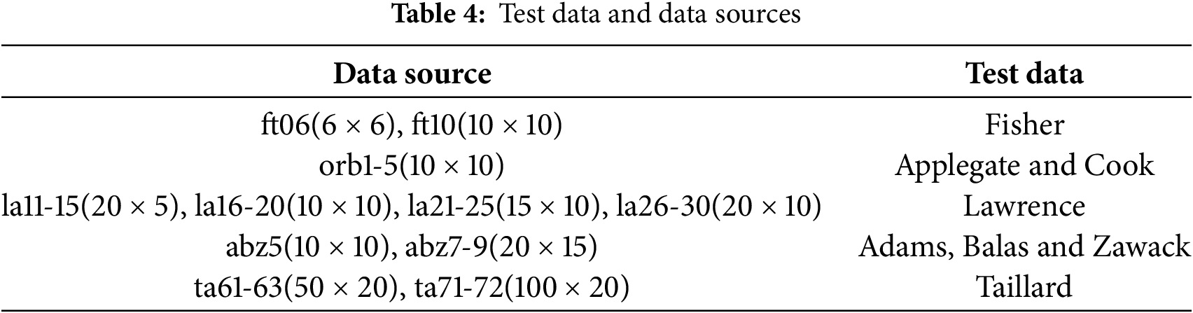
This chapter will evaluate the performance of the proposed job scheduling decision model by simulating both static and dynamic job scheduling environments. We will use classic scheduling data from the OR-library as a benchmark. Details regarding the specific test data, scale, and sources are presented in Table 4 below.

6.1 Algorithm Parameter Settings

This section outlines parameter settings used in model training. Key parameters for decision iteration, neural network hyperparameters, and reinforcement learning updates are listed in Table 5. We set 1000 training episodes, a replay pool size of 60000, and a batch size of 256. The target network updates every 200 steps, using the Adam optimizer with a learning rate of 0.0001.

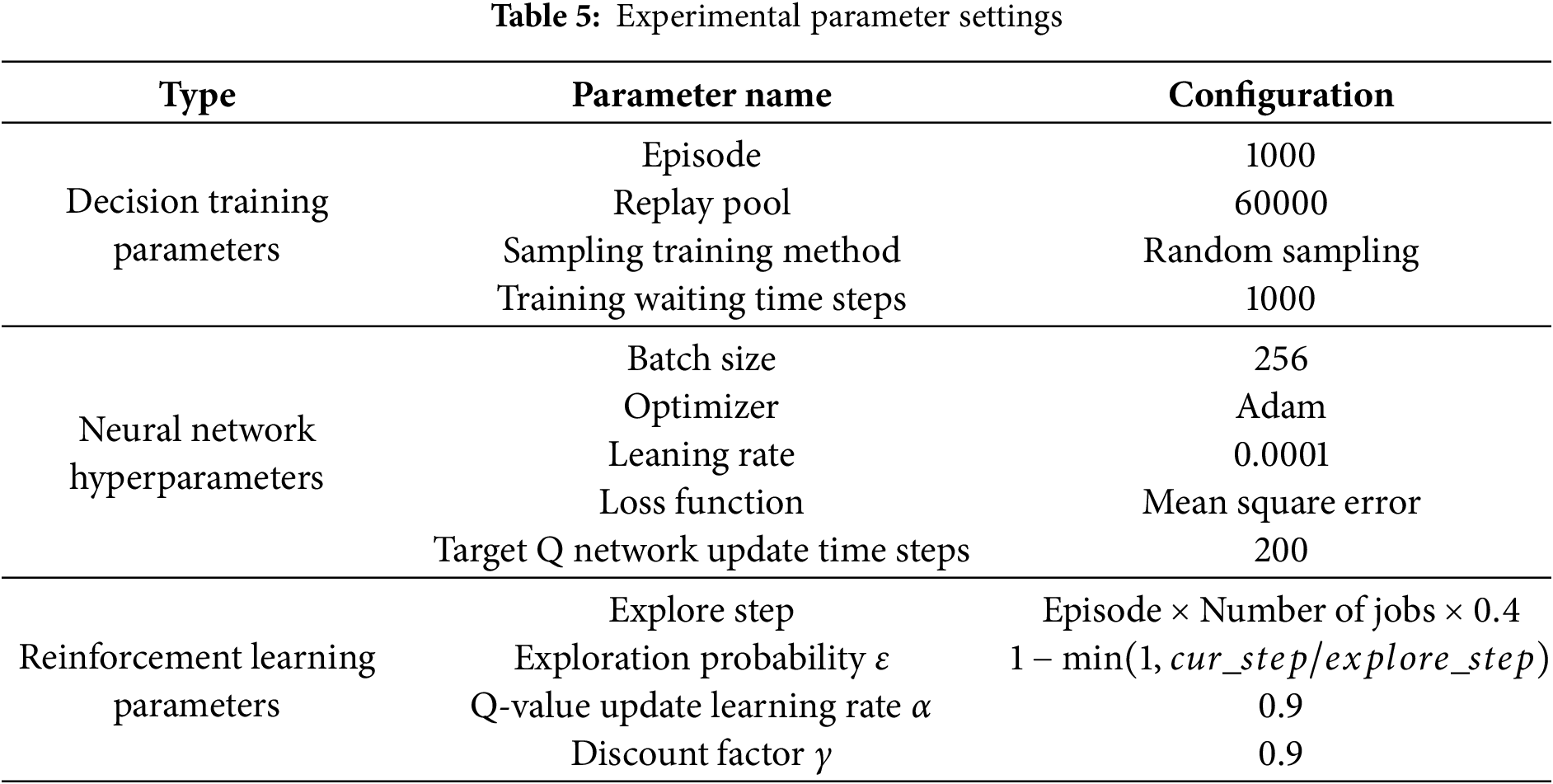
Exploration spans 40% of training, with ε decaying linearly. The learning rate and discount factor are both 0.9. For larger datasets like ta61 and ta71, the cur_policy strategy is enabled when ε<0.2 to accelerate training.

6.2 Model Convergence Analysis

This section evaluates the convergence of the decision model using the maximum scheduling completion time (makespan) as a criterion, with the benchmark abz5 chosen for testing. Results will be analyzed under different settings, including various batch data sizes, sampling training methods, exploration patterns, and numbers of scheduling rules.

To evaluate convergence without labeled data, makespan is used as a proxy loss. Over 1000 training rounds, average performance per 20-round period is reported.

Fig. 6a shows that larger batch sizes (e.g., batch256) enhance convergence speed and stability, especially under the cur_policy strategy. Fig. 6b indicates cur_policy accelerates convergence with more stable outcomes, while ε-greedy achieves better peak scores. Fig. 6c compares sampling methods, where prioritized experience replay improves convergence smoothness and reduces variance but increases training time and reduces sample diversity. Fig. 6d shows that excluding weaker rules (action8) prevents long completion times, confirming the positive impact of combining diverse rules.

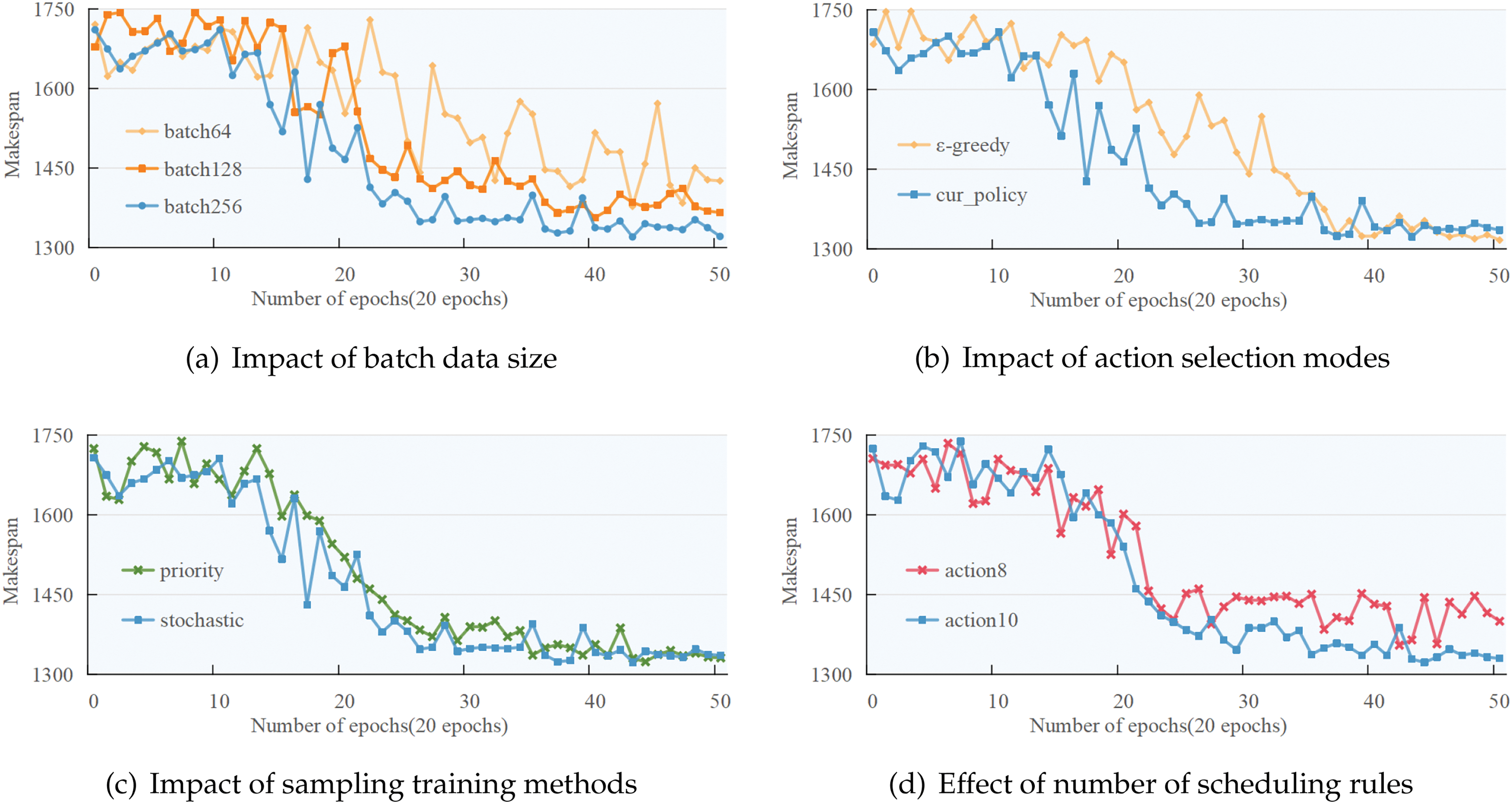
Figure 6: Convergence analysis plot under different parameter conditions

6.3 Experimental Results Comparative Analysis

Section 5 defines the model’s output as the scheduling rule best suited to the current situation. This section compares each scheduling rule’s performance. Table 6 presents results on small-scale benchmarks (6 × 6, 10 × 10, 20 × 5, and 15 × 10), evaluated against the optimal scheduling outcomes.

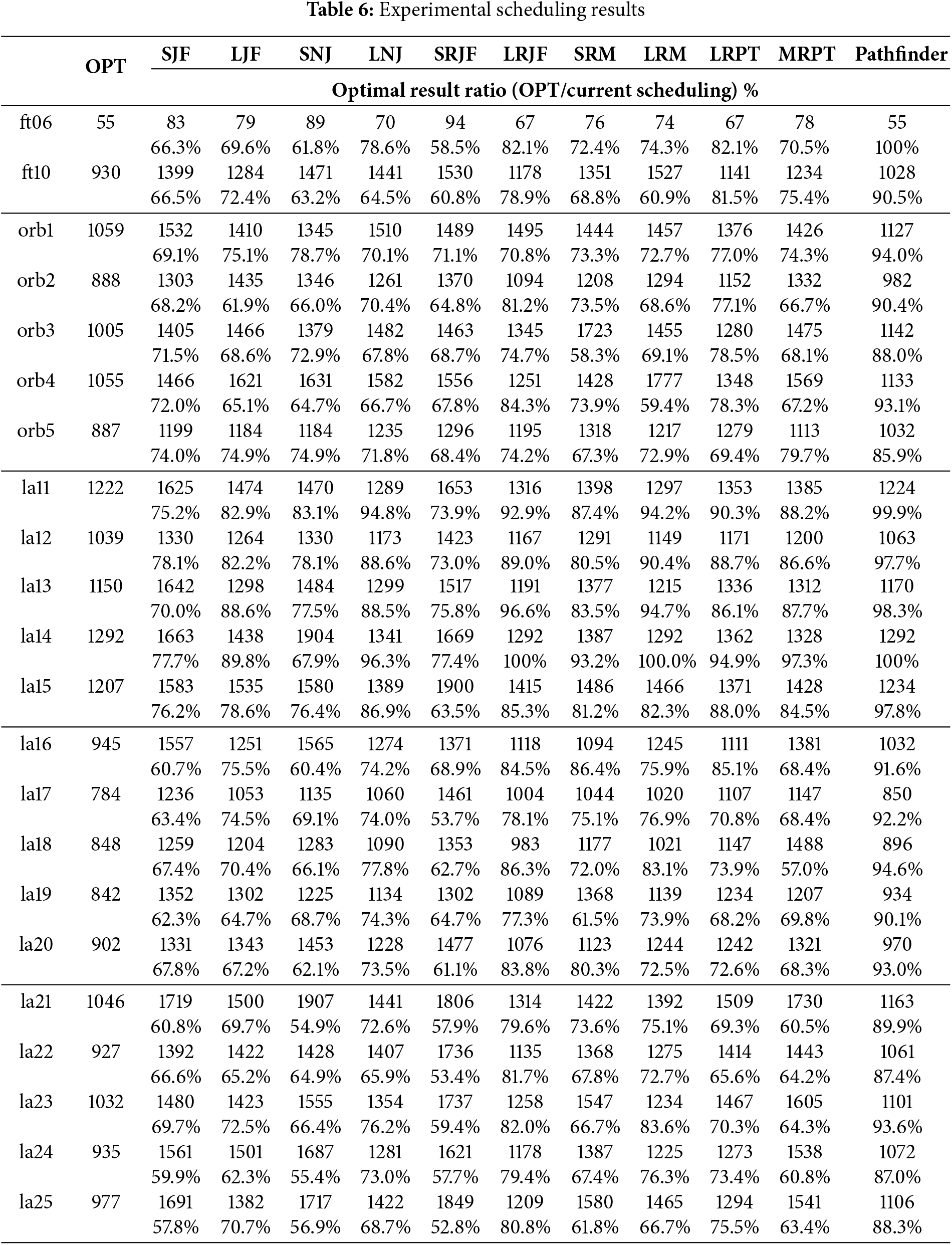
Table 7 shows the best performance of individual scheduling rules across benchmarks. LRJF consistently ranks highest, followed by LRPT, while others perform well only in specific cases. Our proposed method outperforms all single rules in terms of maximum completion time on small to medium-scale benchmarks. A paired t-test confirms it achieves at least 90% of optimal performance (p = 0.013), indicating statistical significance. Fig. 7 shows Pathfinder’s robot utilization closely matches OPT and significantly exceeds the Best Rule, confirming its overall effectiveness.

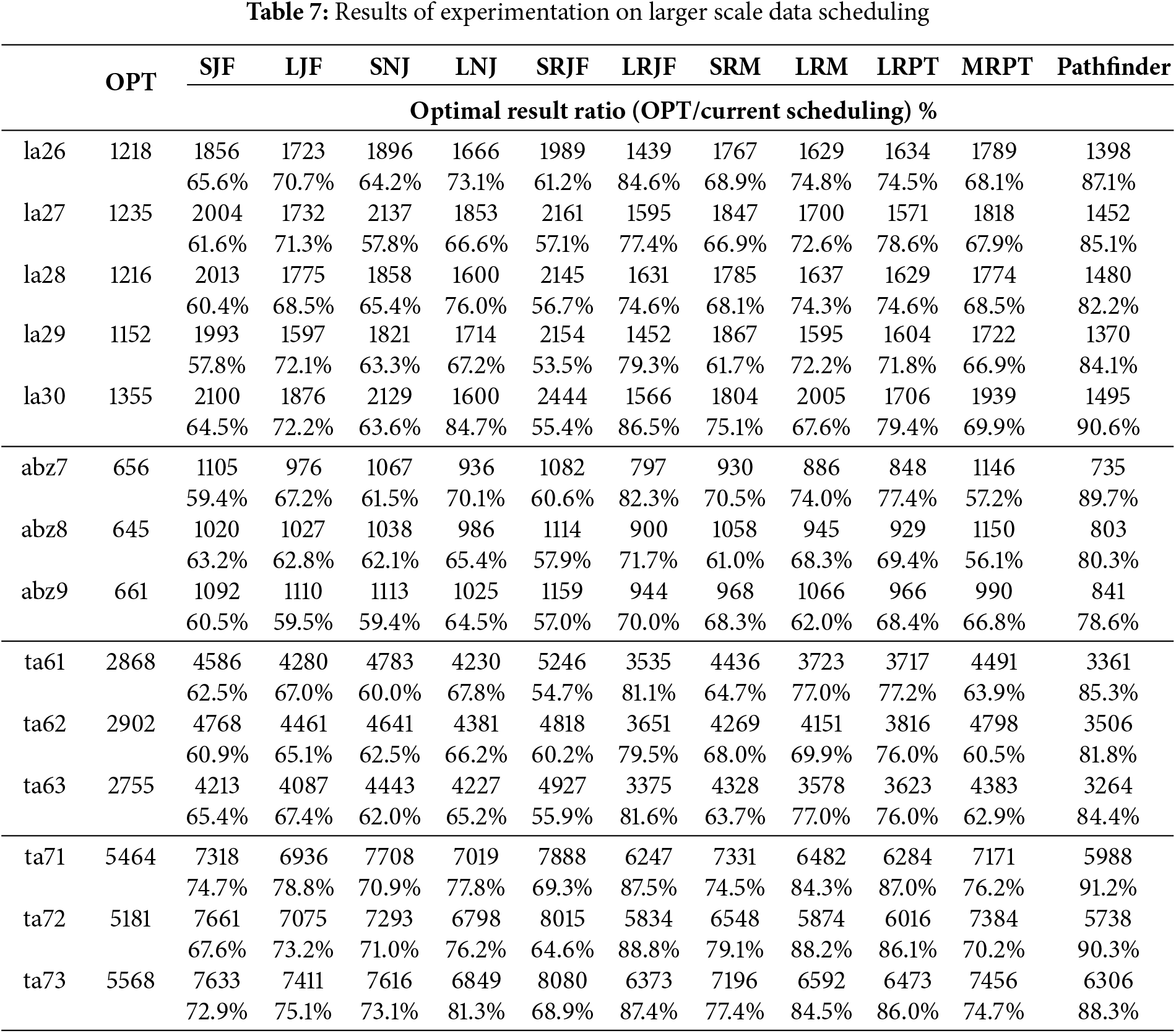
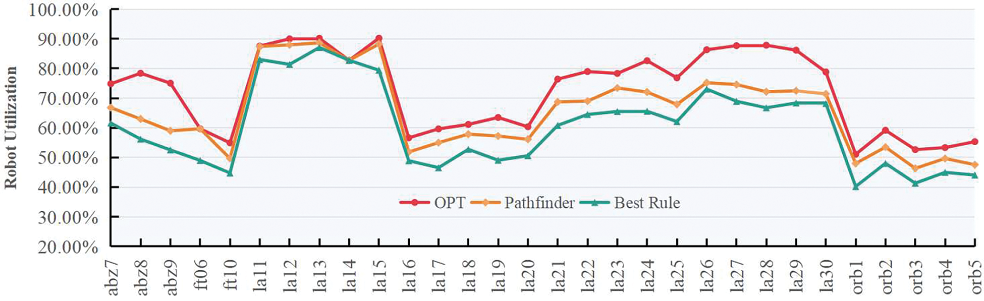
Figure 7: Comparison of utilization among OPT, Best Single Rule and Pathfinder

The model’s performance on larger-scale datasets (Table 7) shows a slight decline compared to smaller-scale results (Table 6), especially in benchmarks like abz8-9, la28, and ta62. This is likely due to increased scenario complexity, suggesting the need for more diverse scheduling rules, as single rules often yield only 60%–70% of the optimal.

A t-test confirms Pathfinder achieves at least 83% of optimal performance (p = 0.032), indicating statistical significance. Fig. 8 compares Pathfinder, Q-learning, and Actor-Critic methods. Pathfinder demonstrates strong performance and stability across scales, consistently approaching optimal solutions more closely than other methods.

Figure 8: Comparison of scheduling performance among various algorithms

Comparison of the maximum completion time ratios shows that Pathfinder, QL, and AC algorithms outperform single optimal rules, following similar trends due to the shared set of ten scheduling rules. Among them, the Actor-Critic algorithm converges fastest but may sacrifice exploration diversity, leading to performance gaps compared to Pathfinder and QL.

QL calculates rewards based on changes in machine utilization and stores Q-values in a table. While effective at small scales, its scalability is limited due to exponential growth in state space, restricting its application to 15 × 10 scheduling. Pathfinder and AC, using neural approximators, avoid this issue.

In conclusion, Pathfinder’s rule-based scheduling achieves superior performance over single rules. However, scheduling quality still depends on rule effectiveness, especially at larger scales. Expanding the rule set may further enhance performance.

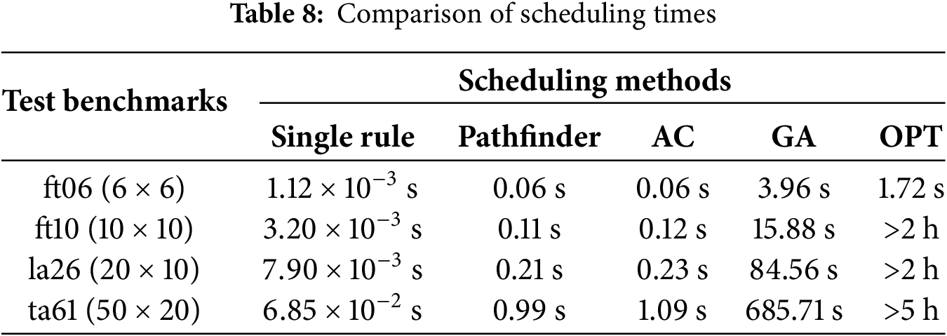
6.4 Decision Time and Robustness

Single scheduling rules exhibit the fastest completion results across all test benchmarks, completing about 20–50 times faster than the Pathfinder algorithm. Both the Pathfinder and AC algorithms demonstrate similar execution times in all benchmarks listed in Table 8. Even when facing scheduling data of size 50 × 20, the Pathfinder algorithm can complete job scheduling within 1 s. However, both the GA algorithm and the optimal results obtained through brute force experience significant increases in scheduling time as the scheduling scale grows, with the solution time of the optimal algorithm becoming intolerable in practical scheduling scenarios.

Real-world scheduling faces uncertainties such as processing time fluctuations and machine failures. Traditional methods like mathematical programming and metaheuristics must re-execute under such changes, incurring extra time costs. In contrast, deep reinforcement learning can adapt to stochastic environments and respond quickly.

We test the trained Pathfinder model on datasets of varying scales with random job and machine seeds. Some job execution times fluctuate by up to 10% to simulate real-world variability. Results, averaged over 100 random datasets, are compared with the AC algorithm and the best single scheduling rule. As shown in Fig. 9, Pathfinder consistently delivers optimal performance across all scales.

Figure 9: Experimental results of random scheduling of data

7  Conclusion

Dynamic customized production introduces complex scheduling challenges. We model it as a multi-stage decision process and propose a deep reinforcement learning approach adaptable to diverse settings. The model achieves over 90% efficiency on small-scale tasks and maintains at least 85% on larger ones, outperforming traditional methods in both speed and adaptability.

Acknowledgement: We would like to thank the College of Computer and Data Science, Fuzhou University, for their technical support and assistance during the research process.

Funding Statement: This work is supported by National Natural Science Foundation of China under Grant No. 62372110, Fujian Provincial Natural Science of Foundation under Grants 2023J02008, 2024H0009.

Author Contributions: The authors confirm contribution to the paper as follows: Conceptualization, Chenxi Lyu; methodology, Chen Dong; software, Qiancheng Xiong; validation, Yuzhong Chen; formal analysis, Qian Weng; data curation, Qiancheng Xiong; writing—original draft preparation, Chenxi Lyu; writing—review and editing, Chenxi Lyu; visualization, Zhenyi Chen; funding acquisition, Yuzhong Chen. All authors reviewed the results and approved the final version of the manuscript.

Availability of Data and Materials: The data that support the findings of this study are available within the article.

Ethics Approval: Not applicable.

Conflicts of Interest: The authors declare no conflicts of interest regarding the present study.

References

1. Jan Z, Ahamed F, Mayer W, Patel N, Grossmann G, Stumptner M, et al. Artificial intelligence for industry 4.0: systematic review of applications, challenges, and opportunities. Expert Syst Appl. 2023;216(9):119456. doi:10.1016/j.eswa.2022.119456. [Google Scholar] [CrossRef]

2. Mia MR, Shuford J. Exploring the synergy of artificial intelligence and robotics in Industry 4.0 applications. J Artif Intell General Sci. 2024;1(1):17–20. [Google Scholar]

3. Daneshmand M, Noroozi F, Corneanu C, Mafakheri F, Fiorini P. Industry 4.0 and prospects of circular economy: a survey of robotic assembly and disassembly. Int J Adv Manufact Techno. 2023;124(9):2973–3000. doi:10.1007/s00170-021-08389-1. [Google Scholar] [CrossRef]

4. Yip M, Salcudean S, Goldberg K, Althoefer K, Menciassi A, Opfermann JD, et al. Artificial intelligence meets medical robotics. Science. 2023;381(6654):141–6. doi:10.1126/science.adj3312. [Google Scholar] [PubMed] [CrossRef]

5. Ryalat M, ElMoaqet H, AlFaouri M. Design of a smart factory based on cyber-physical systems and Internet of Things towards Industry 4.0. Appl Sci. 2023;13(4):2156. doi:10.3390/app13042156. [Google Scholar] [CrossRef]

6. Soori M, Arezoo B, Dastres R. Internet of things for smart factories in Industry 4.0, a review. Int Things Cyber-Phys Syst. 2023;3:192–204. doi:10.1016/j.iotcps.2023.04.006. [Google Scholar] [CrossRef]

7. Yu W, Liu Y, Dillon T, Rahayu W, Mostafa F. An integrated framework for health state monitoring in a smart factory employing IoT and big data techniques. IEEE Int Things J. 2021;9(3):2443–54. doi:10.1109/jiot.2021.3096637. [Google Scholar] [CrossRef]

8. Kalempa VC, Piardi L, Limeira M, de Oliveira AS. Multi-robot task scheduling for consensus-based fault-resilient intelligent behavior in smart factories. Machines. 2023;11(4):431. doi:10.3390/machines11040431. [Google Scholar] [CrossRef]

9. Alpala LO, Quiroga-Parra DJ, Torres JC, Peluffo-Ordóñez DH. Smart factory using virtual reality and online multi-user: towards a metaverse for experimental frameworks. Appl Sci. 2022;12(12):6258. doi:10.3390/app12126258. [Google Scholar] [CrossRef]

10. Büchi G, Cugno M, Castagnoli R. Smart factory performance and Industry 4.0. Technol Forecast Soc Change. 2020;150(3):119790. doi:10.1016/j.techfore.2019.119790. [Google Scholar] [CrossRef]

11. Osterrieder P, Budde L, Friedli T. The smart factory as a key construct of Industry 4.0: a systematic literature review. Int J Prod Econ. 2020;221(4):107476. doi:10.1016/j.ijpe.2019.08.011. [Google Scholar] [CrossRef]

12. Arents J, Greitans M. Smart industrial robot control trends, challenges and opportunities within manufacturing. Appl Sci. 2022;12(2):937. doi:10.3390/app12020937. [Google Scholar] [CrossRef]

13. Lei J, Hui J, Chang F, Dassari S, Ding K. Reinforcement learning-based dynamic production-logistics-integrated tasks allocation in smart factories. Inte J Product Res. 2023;61(13):4419–36. doi:10.1080/00207543.2022.2142314. [Google Scholar] [CrossRef]

14. Hussain RF, Salehi MA. Resource allocation of industry 4.0 micro-service applications across serverless fog federation. Future Generat Comput Syst. 2024;154(2):479–90. doi:10.1016/j.future.2024.01.017. [Google Scholar] [CrossRef]

15. Flores-García E, Jeong Y, Liu S, Wiktorsson M, Wang L. Enabling industrial internet of things-based digital servitization in smart production logistics. Int J Product Res. 2023;61(12):3884–909. doi:10.1080/00207543.2022.2081099. [Google Scholar] [CrossRef]

16. Tricomi G, Scaffidi C, Merlino G, Longo F, Puliafito A, Distefano S. A resilient fire protection system for software-defined factories. IEEE Int Things J. 2021;10(4):3151–64. doi:10.1109/jiot.2021.3127387. [Google Scholar] [CrossRef]

17. Shi Z, Xie Y, Xue W, Chen Y, Fu L, Xu X. Smart factory in Industry 4.0. Syst Res Behav Sci. 2020;37(4):607–17. doi:10.1002/sres.2704. [Google Scholar] [CrossRef]

18. Baker KR, Trietsch D. Principles of sequencing and scheduling. Hoboken, NJ, USA: John Wiley & Sons; 2013. [Google Scholar]

19. Cebi C, Atac E, Sahingoz OK. Job shop scheduling problem and solution algorithms: a review. In: 2020 11th International Conference on Computing, Communication and Networking Technologies (ICCCNT); 2020 Jul 1–3. Kharagpur, India: IEEE; 2020. p. 1–7. [Google Scholar]

20. Marzia S, AlejandroVital-Soto, Azab A. Automated process planning and dynamic scheduling for smart manufacturing: a systematic literature review. Manufact Letters. 2023;35:861–72. doi:10.1016/j.mfglet.2023.07.013. [Google Scholar] [CrossRef]

21. Wang J, Liu Y, Ren S, Wang C, Ma S. Edge computing-based real-time scheduling for digital twin flexible job shop with variable time window. Robot Comput Integr Manuf. 2023;79:102435. doi:10.1016/j.rcim.2022.102435. [Google Scholar] [CrossRef]

22. Sharif Z, Tang Jung L, Ayaz M, Yahya M, Pitafi S. Priority-based task scheduling and resource allocation in edge computing for health monitoring system. J King Saud Univ-Comput Inform Sci. 2023;35(2):544–59. doi:10.1016/j.jksuci.2023.01.001. [Google Scholar] [CrossRef]

23. Um J, Gezer V, Wagner A, Ruskowski M. Edge computing in smart production. In: Advances in Service and Industrial Robotics: Proceedings of the 28th International Conference on Robotics in Alpe-Adria-Danube Region (RAAD 2019) 28. Cham, Switzerland: Springer; 2020. p. 144–52. [Google Scholar]

24. Mangalampalli S, Karri GR, Kose U. Multi objective trust aware task scheduling algorithm in cloud computing using whale optimization. J King Saud Univ-Comput Inform Sci. 2023;35(2):791–809. doi:10.1016/j.jksuci.2023.01.016. [Google Scholar] [CrossRef]

25. Baroudi U, Alshaboti M, Koubaa A, Trigui S. Dynamic multi-objective auction-based (DYMO-auction) task allocation. Appl Sci. 2020;10(9):3264. doi:10.3390/app10093264. [Google Scholar] [CrossRef]

26. Dutta A, Czarnecki E, Ufimtsev V, Asaithambi A. Correlation clustering-based multi-robot task allocation: a tale of two graphs. ACM SIGAPP Appl Comput Rev. 2020;19(4):5–16. doi:10.1145/3381307.3381308. [Google Scholar] [CrossRef]

27. Wei C, Ji Z, Cai B. Particle swarm optimization for cooperative multi-robot task allocation: a multi-objective approach. IEEE Robot Automa Letters. 2020;5(2):2530–7. doi:10.1109/lra.2020.2972894. [Google Scholar] [CrossRef]

28. Yun WJ, Kim JP, Jung S, Kim JH, Kim J. Quantum multi-agent actor-critic neural networks for internet-connected multi-robot coordination in smart factory management. IEEE Internet Things J. 2023;10(11):9942–52. doi:10.1109/jiot.2023.3234911. [Google Scholar] [CrossRef]

29. Zhang JD, He Z, Chan WH, Chow CY. DeepMAG: deep reinforcement learning with multi-agent graphs for flexible job shop scheduling. Knowl Based Syst. 2023;259(5):110083. doi:10.1016/j.knosys.2022.110083. [Google Scholar] [CrossRef]

30. Han BA, Yang JJ. Research on adaptive job shop scheduling problems based on dueling double DQN. IEEE Access. 2020;8:186474–95. doi:10.1109/access.2020.3029868. [Google Scholar] [CrossRef]

31. Zhou T, Tang D, Zhu H, Zhang Z. Multi-agent reinforcement learning for online scheduling in smart factories. Robot Comput Integr Manuf. 2021;72(2):102202. doi:10.1016/j.rcim.2021.102202. [Google Scholar] [CrossRef]

32. Ma H, Li R, Zhang X, Zhou Z, Chen X. Reliability-aware online scheduling for DNN inference tasks in mobile edge computing. IEEE Internet Things J. 2023;10(13):11453–64. doi:10.1109/jiot.2023.3243266. [Google Scholar] [CrossRef]

33. Zhang Y, Zhu H, Tang D, Zhou T, Gui Y. Dynamic job shop scheduling based on deep reinforcement learning for multi-agent manufacturing systems. Robot Comput Integr Manuf. 2022;78(3):102412. doi:10.1016/j.rcim.2022.102412. [Google Scholar] [CrossRef]

34. Liu R, Piplani R, Toro C. Deep reinforcement learning for dynamic scheduling of a flexible job shop. Int J Product Res. 2022;60(13):4049–69. doi:10.1080/00207543.2022.2058432. [Google Scholar] [CrossRef]

35. Alexopoulos K, Mavrothalassitis P, Bakopoulos E, Nikolakis N, Mourtzis D. Deep reinforcement learning for selection of dispatch rules for scheduling of production systems. Appl Sci. 2024;15(1):232. doi:10.3390/app15010232. [Google Scholar] [CrossRef]

36. Gui Y, Tang D, Zhu H, Zhang Y, Zhang Z. Dynamic scheduling for flexible job shop using a deep reinforcement learning approach. Comput Indust Eng. 2023;180:109255. doi:10.1016/j.cie.2023.109255. [Google Scholar] [CrossRef]

37. Li F, Lang S, Hong B, Reggelin T. A two-stage RNN-based deep reinforcement learning approach for solving the parallel machine scheduling problem with due dates and family setups. J Intell Manufact. 2024;35(3):1107–40. doi:10.1007/s10845-023-02094-4. [Google Scholar] [CrossRef]