An SAC-AMBER Algorithm for Flexible Job Shop Scheduling with Material Kit

1  Introduction

With the continuous development of the manufacturing, production, and energy industries, scheduling problems have received increasing attention in recent years [1,2]. It is primarily divided into the Job Shop Scheduling Problem (JSP) and the Flow Shop Scheduling Problem (FSP) [3]. JSP, a classic manufacturing scheduling problem, aims to allocate tasks for multiple workpieces under resource constraints to optimize efficiency [4]. Compared with the job-shop scheduling problem, the Flexible Job-shop Scheduling Problem (FJSP) relaxes the restrictions on machines so that each operation can be processed on multiple compatible machines for each job, which makes FJSP more flexible and sophisticated [5]. Traditional FJSP optimization typically focuses on minimizing makespan [6], for example, in the production of bearings, which are mainly composed of inner rings, outer rings, rollers, and cages, if one of the parts is missing, the assembly cannot be carried out, which will prolong the assembly time, and there will be a risk of not being able to deliver on time. Another example is in the aircraft processing parts process, the lack of any one part will lead to belonging to the same kit or assembly of all parts processing lag, and the subsequent welding assembly can not be carried out [7]. Thus, it is clear that the production of parts in complete sets is critical to assembly-based manufacturing. FJSP with material kit constraints needs to consider the parts in the optimization process, so that all the relevant parts can be completed as synchronously as possible to meet the assembly requirements, compared with the traditional FJSP only focuses on processing efficiency, its scheduling is more complex and close to the actual production. Therefore, it is a challenge to optimize production efficiency by making the part-alignment requirement one of the constraints of FJSP.

Most of the current researches use heuristic algorithms, meta-heuristic algorithms, and deep reinforcement learning methods to solve FJSP problems with constraints such as fuzzy processing time, new job insertion, and machine unavailability.

Many researchers have proposed using heuristic algorithms to solve the FJSP. Ding et al. [8] employed a Fluid Randomized Adaptive Search Algorithm (FRASA) to address the FJSP with fluid dynamic characteristics. Lim and Moon [9] introduced a two-stage iterative mathematical programming-based heuristic approach, utilizing a decomposition scheme that prioritizes operation allocation to minimize the makespan. Boudjemline et al. [10] investigated a multi-objective FJSP aiming to simultaneously minimize the makespan, maximum machine load, and total workload and proposed a genetic algorithm applicable across various fields using spreadsheets. Typically, due to the complexity and flexibility of flexible job shops, heuristic algorithms do not perform well in solving FJSP.

However, in some studies, metaheuristic algorithms have demonstrated superior capabilities in solving flexible job scheduling problems. Fan et al. [11] proposed a hybrid Jaya algorithm integrated with Tabu search, which employs an incremental parameter setting strategy and period estimation to accelerate the spatial search process while ensuring a sufficiently large search space. Liao et al. [12] utilized the ABC II metaheuristic algorithm to solve FJSP with additional resource constraints. Hu et al. [13] addressed the flexible assembly job shop scheduling problem considering energy consumption and environmental pollution using a multi-objective artificial bee colony algorithm. Han and Gong [14] proposed an FJSP model that considers the worker learning forgetting effect and worker collaboration, and solved this bi-objective scheduling problem using a hybrid algorithm based on the nondominated hierarchy; Wang et al. [15] constructed a comprehensive scheduling model that contains four objectives, and proposed an improved decomposed multi-objective evolutionary algorithm to solve the problem; Feng et al. [16] proposed a multi-objective FJSP model containing machine failures, emergency order insertion, and designed an improved NSGA-III algorithm for dynamic scheduling. Although traditional multi-objective evolutionary algorithms can obtain excellent Pareto solution sets, they usually require a large number of computations and are difficult to be adjusted in real time during the production process. For multi-objective trade-offs, some methods use fixed weight combinations or hierarchical indexes, which are often difficult to flexibly adjust the relationship between objectives in practical applications.

Grumbach et al. [17] proposed combining Deep Reinforcement Learning (DRL) and metaheuristic algorithms to solve the Dual-Resource Constrained Flexible Job Shop Scheduling Problem (DRC-FJSSP) with practical orientation. Song et al. [18] addressed the stochastic economic lot scheduling problem by proposing a DRL approach that learns dynamic scheduling policies for SELSP in an end-to-end manner. Lei et al. [19] proposed an end-to-end hierarchical reinforcement learning framework for the large-scale dynamic flexible job shop scheduling problem. In this framework, high-level intelligences classify the DFJSP as a static FJSP subproblem, and two low-level intelligences are responsible for job operation sequencing and machine assignment tasks, respectively; Wu et al. [20] proposed a two-tier DDQN framework for dynamic FJSP for real-time selection of scheduling rules and simultaneous optimization of the sum of job delays and the maximal completion time; Xu et al. [21] designed a dynamic environment containing multiple perturbation events and used a two-tier integrated DQN to optimize maximum completion time, average equipment utilization, and average job drag time, respectively. However, when solving multi-objective problems, the DRL methods studied above often set multiple reward functions to balance each metric, or design multi-layer intelligences to train on multi-objectives, which will increase the complexity of constructing DRL reward functions, state spaces, and intelligences.

The research on FJSP with material kit is less studied at present. Xu et al. [22] constructed a corresponding mathematical model for the processing-assembly cooperative scheduling problem in a composite parallel production line environment by considering the matching constraints; Qiu et al. [23] faced the on-line scheduling problem of a two-phase flexible assembly flow shop by considering the complex constraints of multi-product deliveries and matching assemblies; Huang et al. [24] proposed a new hybrid distribution model for the material distribution scheduling of assembly lines. However, most of these researches adopt a two-stage hierarchical construction of mathematical models in order to ensure the synergy of part assembly, which may lead to the inconsistency of the objectives of the two phases, which will complicate the trade-off mechanism and increase the complexity of the model, and the need to solve the sub-objectives of each phase before solving the overall objective will increase the computational process, which may lead to the deterioration of the quality of the solution.

From the above literature, current FJSP research focuses on dynamic constraints such as fuzzy processing time, new job insertion and machine unavailability, but workpiece flush production often has a large impact on the start time of the next stage of production, so it is necessary to consider workpiece production flush in the production process, even though a small number of studies have mentioned the conditions of flush production in the process of considering the assembly production, but these studies mainly constructed two-stage mathematical models for the assembly stage, which will increase the complexity of the model; meanwhile, in the study of multi-objective FJSP process, many researchers have faced problems such as the need for a large number of computations and multi-objective trade-offs, although they have used multi-objective heuristic and meta-heuristic algorithms to improve the scheduling performance at the same time. And while DRL methods have the advantage of being able to respond quickly to the objectives when solving multi-objective problems, they tend to set more reward functions and intelligences that increase the difficulty of constructing Markov decisions.

To summarize, few scholars have studied the FJSP problem for workpiece flush production, and most of the studies on solving multi-objective problems using DRL with the construction of multi-stage, multi-intelligent body, and multi-reward function, but it will increase the computational process. Therefore, this study integrates part flushness into the scheduling model, considers the multi-objectives of minimizing the maximum part completion time and minimizing the variance of the part completion time, and combines the two optimization objectives into a composite metric by using weighted summation. In terms of objective trade-offs, the weighted summation method fuses the two objectives into a single reward function so that the DRL intelligences can automatically learn to balance the objective weights during the training process instead of fixing the weights beforehand or simply seeking the Pareto frontiers, and the trained DRL strategies can quickly respond online without re-running time-consuming multi-objective optimization algorithms; meanwhile, this study proposes a SAC-based improvement method an Adaptive Multi-Buffer Experience Replay(AMBER) algorithm, which designs three experience buffers for the FJSP problem, and can alleviate the reward sparsity of SAC algorithm while being able to provide more effective strategies for the intelligentsia. Finally, the feasibility of the proposed method and model is verified by setting up experiments on Hurink, Brandimarte and Dauzere benchmarks. The main contributions of this paper are as follows:

(1)   A flexible job shop scheduling model is designed to incorporate kit production requirements among jobs.

(2)   The AMBER experience replay buffer algorithm is proposed, which classifies and manages experiences of varying importance in the Soft Actor-Critic (SAC) framework by designing three distinct buffers: a standard buffer, a high equipment utilization buffer, and a high productivity buffer. This approach addresses the issues of low experience utilization and learning efficiency during training.

(3)   In this study, the improved algorithm is initially trained on the Hurink dataset and fine-tuned on the Brandimarte dataset, demonstrating its effectiveness across different datasets. Additionally, the feasibility of the model under kit production constraints is further validated by randomly sampling data from the Hurink and Dauzere datasets.

The paper is organized as follows: Section 2 describes a Kit Production-Oriented Flexible Job Shop Scheduling Model. Section 3 demonstrates a SAC-AMBER algorithm for FJSP. Section 4 shows the experiment and analysis. Section 5 concludes the paper.

2  Kit Production-Oriented Flexible Job Shop Scheduling Model

2.1 Problem Description

In the Flexible Job Shop Scheduling Problem (FJSP), the production process involves N jobs{J1, J2, ···, JN}, each consisting of P operations{O1, O2, ···, OP}. Each operation can be processed on any one of multiple available machines{M1, M2, ···, MA} [25]. In FJSP, all jobs are multi-operation and multi-job: the shop floor contains multiple jobs, and each job comprises multiple operations [26]. The machines are selective, meaning each operation can be processed on multiple machines, and different machines may have varying processing times. Therefore, we must consider not only the sequence of operations but also the selection of appropriate machines for each operation [27]. At any given time, as long as the primary resources permit, different operations can be processed on different machines simultaneously.

For the FJSP, some basic assumptions should be satisfied:

(1)   All jobs are available for processing at time zero.

(2)   A machine can process only one job at a time.

(3)   Once the processing of an operation for a job starts, it cannot be interrupted.

(4)   There are no precedence constraints between different jobs.

(5)   All jobs have the same priority.

(6)   For the same job, the next operation cannot start until the previous operation is completed.

2.2 Kit Production-Oriented Flexible Job Shop Scheduling Model

As shown in Table 1, the variable list provides the definitions of each variable used in the formulas.

In the actual production process, a finished product is usually assembled from multiple parts. Therefore, in order to ensure the readiness of sets of parts in the assembly process, it is necessary to consider the balance of multiple product completion times in the production scheduling process. To address this issue, this study introduces a dual optimization objective that aims to more fully reflect the complexity and diversity of the actual production environment. The objective of minimizing the maximum completion time alone may lead to serious deviations in the completion time of certain operations, which in turn delays the subsequent assembly. Although making the material kit as a constraint can alleviate this problem, it is difficult to strictly satisfy this constraint in complex manufacturing environments, and it will limit the flexibility of the scheduling strategy and reduce the diversity of the solution space and the availability of optimal solutions. Therefore, in this study, the optimization objectives are set to minimize the production cycle time and reduce the completion time variance of different kits of products as shown in Eqs. (1) and (2). The multi-objective optimization approach helps to achieve the trade-off between different scheduling objectives and better cope with the uncertainty in the actual production.

F1=Cmax(1)

F2=Var(Gg)(2)

AVGg=1|Gg|∑p∈GgCp(3)

Var(Gg)=1|Gg|∑p∈Gg(Cp−AVGg)2(4)

The constraints are expressed as follows:

s.t.

tpkl>0,Spk≥0,∀p,k,l(5)

Cp<Cmax,∀p(6)

Ml∈M,∀l(7)

∑h∈Mpkxpkh=1,∀p,k(8)

Epk−Spk≥tpkl,∀p,k,h(9)

(Epk−tpkh−Epk−1)xpkh≥0,∀p,k,h(10)

(Eab−tabh−Epk)xpkhxabh(ypkab+1)+(Epk−tpkh−Eab)xpkhxabh(1−ypkab)≥0,∀p,k,a,b,h(11)

Eq. (5) indicates that the processing time of all operations is greater than 0, and processing can start at time zero on the machines; Eq. (6) ensures that the completion time of the last operation of each job does not exceed the makespan; Eq. (7) states that all machines are included in the machine set. Eq. (8) specifies that each operation of each job can be assigned to only one machine for processing; Eq. (9) defines the completion time of an operation minus its start time as greater than or equal to its processing time; Eq. (10) requires that operations assigned to the same machine must follow a sequential order; Eq. (11) ensures that each machine can process only one operation at any given time.

3  Deep Reinforcement Learning with SAC-AMBER for Flexible Job Shop Scheduling

3.1 Deep Reinforcement Learning with SAC

Reinforcement learning (RL) enables an agent to learn and achieve goals by interacting with the environment [28]. The agent selects actions based on the current state and adjusts its strategy through environmental rewards, aiming to maximize cumulative rewards. RL problems are typically modeled using Markov Decision Processes (MDPs), defined by the tuple <S, A, P, r, γ>, where S is the state set, A is the action set, P is the transition function, r is the reward function, and γ is the discount factor [29].

In deep RL, Soft Actor-Critic (SAC) is an off-policy algorithm combining maximum entropy learning with the Actor-Critic framework. SAC optimizes an entropy-regularized objective, maintaining policy randomness to enhance robustness and generalization. SAC has been successfully applied in various domains: Some researchers used SAC to maximize energy management systems; Some researchers designed a discrete decision-making strategy based on Discrete Soft Actor-Critic with Sample Filtering (DSAC-SF) for highway driving efficiency and safety; Some researchers proposed a multi-agent actor-critic approach with a heuristic attention mechanism for multi-agent pathfinding; and Some researchers applied SAC to intelligent passively mode-locked fiber laser (PMLFL) systems. However, its application to flexible job shop scheduling problems (FJSP) remains unexplored. This study extends SAC to discrete action spaces and proposes a novel experience replay method tailored for FJSP. Optimizing the sampling mechanism enhances SAC’s exploration capability in complex scheduling environments, offering a new solution for FJSP.

3.2 Design of an Adaptive Multi-Buffer Experience Replay Mechanism (AMBER)

For off-policy reinforcement learning, the experience replay buffer stores past interactions between the agent and the environment, enabling the agent to learn from historical data rather than relying solely on new data generated by the current policy [30]. However, traditional experience replay typically employs a single replay buffer, where experiences are stored sequentially without distinguishing their importance. This often results in the overwriting of critical experiences [31]. To address these limitations, we propose the use of AMBER (Adaptive Multi-Buffer Experience Replay) as a replacement for the traditional experience replay buffer.

The AMBER (Adaptive Multi-Buffer Experience Replay) algorithm improves off-policy reinforcement learning by introducing three buffers: the Standard Experience Buffer (SEB), the High Utilization Experience Buffer (HUEB), and the High Productivity Experience Buffer (HPEB). SEB stores all experiences for diversity, while HUEB and HPEB store critical experiences where equipment utilization exceeds threshold ϵ and productivity exceeds threshold η, respectively. At the end of each episode, AMBER classifies experiences into the corresponding buffers based on utilization and productivity, with all experiences stored in SEB. During training, AMBER samples from SEB, HUEB, and HPEB using dynamically adjusted ratios λ and β, prioritizing HUEB and HPEB to accelerate convergence and enhance learning efficiency.

The parameters ϵ and η can be dynamically adjusted based on information entropy thresholds.

The empirical distribution entropy of equipment utilization and productivity is initially computed, as expressed in Eqs. (12) and (13).

H(U)=−∑p(u)log⁡p(u)(12)

H(P)=−∑p(p)log⁡p(p)(13)

here, U denotes the set of equipment utilization rates, p(u) represents the probability distribution of utilization u, and H(U) is the entropy of equipment utilization. Similarly, P denotes the set of productivity values, p(p) is the probability distribution of productivity p, and H(P) is the corresponding entropy.

ε, η update formula, as shown in Eqs. (14) and (15):

εt+1=εt+b⋅H(U)(14)

ηt+1=ηt+b⋅H(U)(15)

here, ϵt and ηt represent the current thresholds for equipment utilization and productivity, respectively, while ϵt+1 and ηt+1 denote the updated thresholds for equipment utilization and productivity. The term b is a tuning coefficient that controls the influence of entropy on threshold adaptation, typically constrained within the range (0, 1).

As shown in Eqs. (16) and (17), the ratios λ and β are adaptively adjusted based on rewards, but it is necessary to ensure that λ and β do not exceed 1. Here, ΔR represents the change in rewards between the current episode and the previous episode, and k is a parameter that controls the adjustment speed.

λnew=λold×(1+k⋅ΔR|R|)(16)

βnew=βold×(1+k⋅ΔR|R|)(17)

3.3 Design of the SAC-AMBER Algorithm for the Flexible Job Shop Scheduling Problem (FJSP)

In this study, the SAC-AMBER algorithm is designed for the Flexible Job Shop Scheduling Problem (FJSP). As shown in Fig. 1, the SAC agent interacts with the environment, receiving experiences {St, Rt, at, St+1}, which are passed to the AMBER buffer. AMBER selects experiences based on predefined ratios and forwards them to the SAC agent network.

Figure 1: Flowchart of the SAC-AMBER algorithm

The pseudo-code for the SAC-AMBER algorithm is designed as follows (Algorithm 1):

In deep reinforcement learning, the state space, action space, reward function, and environment are critical components. The environment primarily involves the modeling of the FJSP problem, including information on the states of jobs and processing units. The following sections focus on the design of the SAC-AMBER algorithm for FJSP, specifically addressing the state space, action space, and reward function.

1.   Design of the State Space

The state is crucial in deep reinforcement learning, as it forms the foundation for the agent’s decision-making and directly influences learning efficiency and generalization capabilities. In the Flexible Job Shop Scheduling Problem (FJSP), the state space is designed at three levels S = [Sa, Sb, Sc]:

Here, Sa = [Sa,1, Sa,2, Sa,3, Sa,4] represents the state related to job features. Sa,1 denotes the machine numbers assigned to all job operations up to the current training step t. Machine numbers are indexed starting from 1, and if an operation is displayed as 0, it indicates that the operation has not yet been assigned a machine for processing. Sa,2 represents the processing times of all job operations up to the current training step t. If no machine has been selected for processing, the value is displayed as 0. Sa,3 indicates the start times of job operations. If a negative value is displayed (since the start time of the first operation could be 0, requiring differentiation), it means the operation has not yet started processing on a machine. Sa,4 represents the completion times of job operations. If a value is displayed as 0, it indicates that the operation has not yet started processing.

Sb = [Sb,1, Sb,2, Sb,3, Sb,4] represents the state related to machine features. Sb,1 indicates the status of each machine, where a value of 1 denotes that the machine has started processing, and 0 otherwise. Sb,2 represents the job operations assigned to each machine. Sb,3 denotes the total processing time each machine has completed so far. Sb,4 represents the utilization rate of each machine up to the current time step t, as shown in Eq. (18), where Tact is the actual processing time of each machine, and Tavl is the available time of each machine up to the current time step t.

MUr=TactTavl(18)

Sc = [Sc,1, Sc,2, Sc,3] represents the global state. Sc,1 indicates the number of remaining operations for each job at the current time step t. If the value is 0, it means the job has been fully processed. Sc,2 represents the total utilization rate of all machines at the current time step t, as shown in Eq. (19). Sc,3 represents the total delay time of all operations on the machines at the current time step, as shown in Eq. (20).

MtotalUr=∑l=1m(Tact×MUr)∑Tavl(19)

Ttotalla=∑l=1m(Tavl−Tact)(20)

2.   Design of the Action Space

In the flexible job shop scheduling problem, the design of the action space is crucial as it directly impacts the decision-making flexibility and scheduling efficiency of the agent. This paper adopts a two-step action design at each time step t, as illustrated in Fig. 2. First, the processing machine is selected for the current operation of each workpiece, determining the machine number and processing time. Then, the workpiece to be processed is selected, and the workpiece number, operation count, and machines to be allocated are identified. Through this design, the agent can effectively balance exploration and exploitation in complex environments, optimizing scheduling objectives and adapting to dynamic changes.

Figure 2: Flowchart of the action space

In the job selection action space, we have chosen four common rules for selecting jobs:

(1)   MTT: Select the job minimizing total processing time.

(2)   SPT: Select the job with the shortest current processing time.

(3)   SSCO: Select the job with the smallest sum of current and next operation processing times.

(4)   SNOPT: Select the job with the shortest processing time for the next operation.

In the machine selection action space, we use four rules:

(1)   SPTCO: Select the machine with the shortest processing time for the current operation.

(2)   LUR: Select the machine with the lowest utilization rate.

(3)   STPTSP: Select the machine with the shortest total processing time so far.

(4)   ECTCO: Select the machine that can complete the current operation as soon as possible.

Instead of directly outputting the corresponding workpiece operations and machine codes, the intelligences in this study output heuristic scheduling rules, which are used to decode the corresponding workpieces and machines based on the current state information, and the combination of the workpiece selection rules and machine selections designed above are combined into a hybrid rule as the action space of the intelligent body, as shown in Fig. 3 (Lines of one color in the figure connect a rule).

Figure 3: Rules of the action space

3.   Design of the Rewards

Since our model aims to minimize the makespan (maximum completion time) and ensure kit production, the reward function is designed as a weighted sum of the makespan and kit production variance. In this study, the makespan and the variance of completion times are normalized separately. Since the normalized values are unbounded, the Tanh function is applied to constrain the normalized data. Finally, the weights are automatically determined, and the objectives are combined into a composite goal. First, the two objective values are normalized as follows:

For each objective fi, where f1 represents the makespan (maximum completion time), and f2 represents the variance of job completion times, the makespan and the variance of completion times are normalized separately at the t times observation as shown in Eq. (21).

fi(t)=fi(t)−μi(t)σi(t)+ω(21)

here, μi(t) is the online mean of objective fi at time step t, and σi(t) is the online standard deviation of objective fi at time step t. ω is a small positive constant used to prevent division by zero.

The exponentially weighted moving average is used to update the mean and standard deviation, where χ ∈ (0, 1) is the smoothing parameter that controls the influence of new data on the statistics, as shown in Eqs. (22) and (23).

μi(t)=(1−χ)μi(t−1)+χfi(t)(22)

σi(t)2=(1−χ)σi(t−1)2+χ(fi(t)−μi(t))2(23)

To prevent the normalized values from becoming excessively large, the Tanh function is applied to constrain the normalized values, ensuring that the processed values fall within the range [−1, 1], as shown in Eq. (24).

fi(t)=tanh⁡(γ⋅fi(t))(24)

Therefore, the reward function is defined as shown in Eq. (25).

r(t)=ψ⋅f1(t)+κ⋅f2(t)(25)

In this objective function, f1(t) represents the makespan (maximum completion time), and f2(t) represents the variance of the completion times of critical kit products. The weights ψ and κ balance the trade-off between scheduling time and variance. To enhance the adaptability of the model, these weights are dynamically adjusted based on gradients during training. During network updates, not only are the network parameters updated, but the objective weights are also optimized.

4  Experiment and Analysis

4.1 Experimental Setup

This study utilizes three test sets of varying scales—Hurink [32], Dauzere [33], and Brandimarte [34]—to validate the feasibility and generalizability of the algorithm. Initially, the algorithm is trained on the Hurink dataset to evaluate its performance across different task scales. Subsequently, training is continued on the Brandimarte dataset to assess its robustness in large-scale and complex scenarios, ensuring stable training effectiveness. Furthermore, to verify the feasibility of the model’s design for completeness, data from the Hurink and Dauzere datasets are extracted and combined for training, further testing the algorithm’s applicability in completeness scenarios. Through comprehensive experiments across multiple datasets, the adaptability and performance of the algorithm are thoroughly validated.

A comparative experiment, as shown in Fig. 4, was designed to investigate the impact of key hyperparameters in the SAC-AMBER algorithm, such as the learning rate, soft update parameter, discount factor, entropy, Experience pool utilization threshold and Experience pool productivity threshold, all other parameters are automatically adjustable according to the training process. Each group of experiments was trained for 500 rounds and the average reward values obtained for different values of the parameters were compared separately. The figure shows that when the learning rate is 0.02, soft update parameter is 0.1, discount factor is 0.003, entropy is 0.003, Experience pool utilization threshold is 0.4 and Experience pool productivity threshold is 0.4, the reward values obtained are relatively stable.

Figure 4: Comparison of parameters

The hyperparameter settings for the SAC-AMBER algorithm are shown in Table 2:

To validate the proposed method, SAC-AMBER is compared with heuristic rules (Rule 1: SPT + STM, Rule 2: EEW + LTM) and DRL algorithms. SPT denotes the shortest processing time, EEW is the earliest end of processing, STM is the machine with the shortest total runtime, and LTM is the machine with the longest total runtime. The Gap is calculated using a formula as shown in Eq. (26), where, Cmax denotes the maximum completion time obtained by the algorithm, and Opt is the optimal solution or approximate optimal solution obtained by the exact method.

Gap=Cmax−OptOpt×100%(26)

The program in this study was executed on a computer with a Windows 10 64-bit operating system. The programming environment was based on Python 3.8, utilizing PyTorch 2.1, and the experiments were conducted on an Intel(R) Core(TM) i5-10400 CPU @ 2.90 GHz.

4.2 Experimental Analysis

4.2.1 Validation of Action Space Rule Effectiveness

In order to verify the validity of the proposed rules in the action space, this study takes MK01 as an example, and only one rule and 16 rules can be randomly selected during the training process are compared, and the maximum completion time is recorded. As shown in Fig. 5 box plot, the random rule in the figure indicates that all rules can be randomly selected in the training process, and Cmax indicates the maximum completion time obtained in the training process.

Figure 5: Box plots of the distribution of completion times for different rules

From the figure it can be seen that all the rules have an effect on the training process, but a single rule does not allow the intelligence to train to find the optimal solution, when all the rules can be chosen randomly, the maximum value of the maximum completion time obtained is smaller, and the maximum completion time values obtained are more concentrated, the median of all the results is smaller, which helps the intelligence to be trained better. Also this study recorded the frequency of each rule being selected under 100, 300, 500 and 700 rounds of training respectively as shown in Fig. 6, where percent indicates the percentage of each rule being selected during the training process.

Figure 6: Different rules for selecting frequency

From the figure, it can be seen that when the number of training times is 100, rule 9 is selected for the most tests, indicating that rule 9 is suitable to be more suitable for the intelligent body to complete the scheduling process in the early stage, and with the increase of the number of training times, the frequency of rule 11 being selected gradually increases until after the number of training times is 500, the intelligent body mainly selects rule 11, indicating that rule 11 is more suitable for the intelligent body to complete the scheduling process in the later stage.

4.2.2 Effectiveness of the AMBER Experience Pool

In order to verify the effectiveness of the proposed empirical pooling, this study designed experiments to train 500 rounds during the training process using one buffer, two buffers, and three buffers, respectively, and recorded the average reward values during the training process, as shown in Fig. 7. In the figure, one buffer indicates that only the standard buffer is used, two buffers indicate that the standard buffer and the high equipment utilization buffer are used, and three buffers indicate that the standard, high equipment utilization, and high productivity buffers are used.

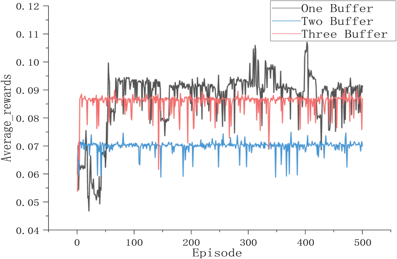
Figure 7: Comparison of different replay buffers

From the figure, it can be seen that when using one buffer, the reward value fluctuates more during the training process and is not smooth enough, when using two buffers, although the reward fluctuation of the training process becomes smaller, the overall reward value also becomes smaller, and the training effect is not good, when using three buffers can ensure that there is a smooth training process under the state of large reward value, and it has a greater improvement in the training of the intelligent body. A higher reward value demonstrates that this method achieves better training performance. The experimental results demonstrate that the three-buffer strategy achieves more stable scheduling performance and better objective values. In terms of overall policy convergence speed, training stability, and generalization ability, the three-buffer configuration clearly outperforms the two-buffer strategy. Therefore, we conclude that the three-buffer mechanism provides more effective training and is better suited for enhancing the performance of the reinforcement learning agent.

4.2.3 Experimental Analysis on the Hurink Dataset

In this study, the la-series datasets from the edata, rdata, and vdata subsets of the Hurink dataset are selected as the training datasets. To provide a clear and concise analysis, eight representative datasets were chosen from a total of 120, covering a wide range of task scales, machine counts, and constraint conditions to reflect the algorithm’s performance across different scenarios comprehensively. The SAC-AMBER algorithm is compared with heuristic rules (Rule 1 and Rule 2) and deep reinforcement learning algorithms (Song et al. [35]; Lei et al. [36]; Yuan et al. [32]), as shown in Table 3. In Table 3, the Cmax column indicates the maximum completion time obtained under the algorithm or rule, The Gap column indicates the percentage difference between the Cmax obtained by the method used and the Opt, and the Opt column indicates the optimal solution of the instance.

As can be seen from Table 4, all algorithms in SAC-AMBER are capable of obtaining the optimal solutions for the current set of instances. However, there are significant differences in how these algorithms optimize the model and make decisions during the training process. To validate the performance of the algorithm under different data sizes, we now categorize the selected datasets based on the size of a × b. If a × b < 100, it is classified as a small dataset; if 100 < a × b < 200, it is classified as a medium dataset; and if a × b > 200, it is classified as a large dataset. Based on this classification, the data is divided as shown in the table below:

In this experiment, one dataset from each of the large, medium, and small datasets is selected. To comprehensively evaluate the performance of the proposed SAC-AMBER algorithm in the FJSP, three representative types of comparative methods are selected for the experiments: heuristic scheduling rules (Rule 1 and Rule 2), classical meta-heuristic algorithms (Genetic Algorithm GA and Particle Swarm Optimization Algorithm PSO), and deep reinforcement learning methods (Deep Q-Network DQN). These methods are widely adopted in FJSP research and serve as strong references due to their representativeness and practical relevance. Heuristic rules are commonly used in real-world production systems for their simplicity and computational efficiency, offering fast and feasible solutions. Meta-heuristic algorithms like GA and PSO are well-known for their global search capability and ease of implementation, making them suitable for solving complex scheduling problems. DQN, as a popular reinforcement learning approach in recent years, has been applied to develop adaptive scheduling strategies with promising performance.

Although the problem addressed in this paper is bi-objective in nature, to align with the training mechanism of reinforcement learning methods, we adopt a weighted summation approach to convert the bi-objective problem into a single-objective optimization model. This approach is commonly used in existing reinforcement learning-based scheduling studies and contributes to training stability and model feasibility [37]. Based on this transformation, to ensure a fair comparison of scheduling performance across different types of algorithms, two classical single-objective meta-heuristic algorithms GA and PSO are selected. These algorithms are widely used in FJSP, have strong search capabilities and engineering practicability, and serve as important baselines for evaluating the effectiveness of new approaches.

The SAC-AMBER algorithm, along with Rule 1, Rule 2, GA, PSO, and DQN, is trained for 500 epochs on each dataset. The scheduling times of the algorithms are then visualized using box plots, as shown in Fig. 8. From the figure, it can be observed that, across all three dataset sizes (large, medium, and small), the SAC-AMBER algorithm achieves a smaller distribution of makespan compared to the other algorithms. The median makespan of SAC-AMBER is lower than that of the other algorithms, demonstrating better stability and training performance.

Figure 8: Box plot comparison of algorithms

As shown in Fig. 9, this paper compares the performance of SAC and SAC_AMBER on three datasets: Vdata01, Vdata26, and Vdata39. The average reward curves of the two algorithms over 500 training epochs show significant differences: SAC_AMBER demonstrates superior convergence characteristics and stability across all three datasets, with its final average reward value improving by approximately 15–25% compared to SAC. Notably, in Vdata26, SAC_AMBER achieves stable convergence after 300 episodes. Experimental results validate the effectiveness of SAC_AMBER in improving exploration strategies through the integration of the AMBER method.

Figure 9: The performance of SAC and SAC_AMBER

Fig. 10 compares the training performance of DQN, SAC_AMBER, and DDPG on three datasets: Vdata01, Vdata21, and Vdata39. SAC_AMBER shows the best convergence speed and stability across all datasets, particularly outperforming DQN and DDPG in the later stages of the large dataset Vdata39. Using Vdata as an example, SAC-AMBER achieves higher and more stable average reward values across large, medium, and small datasets in the Rdata, Edata, and Vdata categories. This demonstrates that SAC-AMBER exhibits higher training stability and superior performance compared to other reinforcement learning algorithms.

Figure 10: Algorithm comparison line plot

4.2.4 Experimental Analysis on the Brandimarte Dataset

In this study, we employ transfer learning to train the model further, which was initially trained on the Hurink dataset, using the entire Brandimarte dataset. The SAC-AMBER algorithm is compared with heuristic rules, and deep reinforcement learning algorithms, as shown in Table 5.

From Table 6, it can be observed that SAC-AMBER, after further training using transfer learning, still achieves the optimal solutions for the given benchmark instances. To validate the algorithm’s performance under different data sizes during continued training, we classify the datasets into small, medium, and large scales, following the same criteria as above. The resulting data classification is presented below.

In this experiment, one dataset from each of the large, medium, and small categories was selected. SAC-AMBER, Rule1, Rule2, GA, PSO, and DQN were trained for 500 iterations on each dataset. The maximum completion times were analyzed and visualized using box plots, as shown in Fig. 11. In MK01, MK03, and MK10 scenarios, SAC-AMBER achieved the lowest median values and narrowest distribution ranges, demonstrating its superiority in minimizing completion time and maintaining stability. Compared to other algorithms, SAC-AMBER consistently delivers optimal and stable results across scenarios.

Figure 11: Box plot comparison of algorithms

This experiment compares the reinforcement learning performance of SAC_AMBER and SAC using three datasets of different scales: MK01, MK03, and MK10, as shown in Fig. 12.

Figure 12: The performance of SAC and SAC_AMBER

The results show that SAC-AMBER consistently outperforms SAC across all environments. In MK01, SAC-AMBER achieves a 23% higher average reward and faster convergence. In MK03, it maintains a steady-state reward above 0.8, while SAC declines after 300 episodes. In MK10, SAC-AMBER remains stable, whereas SAC oscillates, highlighting its adaptability to non-stationary state spaces. These findings confirm SAC-AMBER’s robustness and superior performance.

To validate the improvements of SAC-AMBER, this study compares it with DQN and DDPG using reward comparison plots. As shown in Fig. 13, SAC-AMBER demonstrates faster convergence and greater stability, exhibiting a more rapid rise in reward curves during the early training phase and maintaining higher stability in high-complexity environments compared to the other two algorithms. By leveraging entropy adaptive adjustment, SAC-AMBER achieves an effective exploration-exploitation balance.

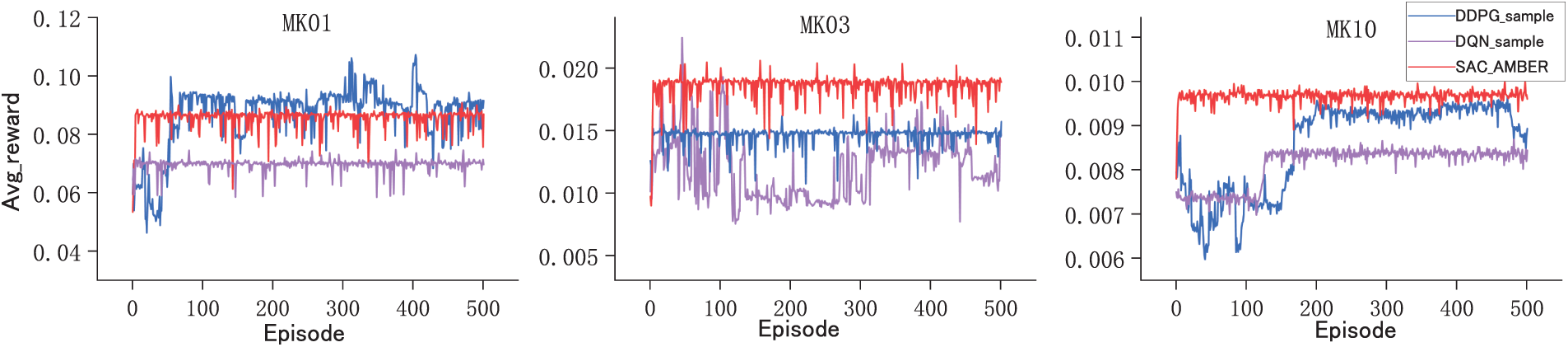
Figure 13: Algorithm comparison line plot

4.2.5 Experimental Analysis on Combined Datasets

In the previous experiments, the effectiveness of the proposed approach in maximizing the minimum completion time was validated. Next, to assess the effectiveness of the model in ensuring job-set completeness, we conducted experiments on combined datasets. Specifically, we selected sub-datasets from the Hurink and Dauzere datasets, ensuring a fixed number of machines while combining different sub-datasets. From each sub-dataset, four rows of data were selected to form a complete dataset, where the four jobs from each sub-dataset exhibited a certain level of completeness. Table 7 presents the variance results of job-set completeness for different algorithms. The GA, PSO, DQN, and DDPG algorithms used in Table 7 for performance comparison all employed the weighted sum method to transform multi-objective optimization into a single-objective problem.

From the results presented in Table 7, SAC-AMBER consistently outperforms GA, PSO, DQN, DDPG, Song et al., Lei et al. and Yuan et al. across datasets like la01, la02, and 01a, showing the lowest variance in job completion times. GA and PSO exhibit higher variance, especially with more machines, while DQN and DDPG perform moderately but still lag behind SAC-AMBER. Song et al., Lei et al. and Yuan et al.’s algorithms are also not as good as SAC-AMBER algorithm in solving the maximum completion time variance. Overall, SAC-AMBER demonstrates superior consistency and stability, particularly in large-scale and complex scheduling tasks, making it the preferred choice for consistency optimization.

To evaluate the generalization capability of the model, we applied the trained SAC-AMBER model directly to the Dauzere dataset, specifically on subsets 07a and 08a, selecting four jobs from each dataset. The corresponding Gantt charts are shown in Fig. 14.

Figure 14: Overall Gantt chart

To better illustrate job-set completeness, Fig. 10 is further divided into Figs. 15 and 16. The results reveal that job assignments on machines are relatively compact, effectively reducing idle times and minimizing the maximum completion time. Additionally, jobs from the same batch are completed at similar times across different machines, indicating strong job-set completeness.

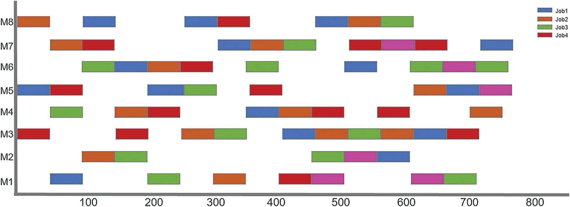
Figure 15: Part 1 Gantt chart

Figure 16: Part 2 Gantt chart

5  Conclusion

This study proposes SAC-AMBER for the Flexible Job Shop Scheduling Problem (FJSP) with job-set completeness constraints. We design a novel scheduling model that optimizes maximum completion time while incorporating job-set completeness constraints to enhance production coordination. To address low experience utilization and slow convergence in reinforcement learning, we introduce the Adaptive Multi-Buffer Experience Replay (AMBER) mechanism, which uses a multi-tiered buffer (standard, high-machine-utilization, and high-productivity) to improve experience utilization, accelerate convergence, and enhance generalization.

Experiments show that SAC-AMBER reduces maximum completion time and optimizes job-set completeness across datasets (Hurink, Brandimarte, Dauzere), outperforming traditional heuristic, metaheuristic, and other DRL methods in efficiency and solution quality, especially in large-scale problems.

This study validates reinforcement learning’s feasibility in FJSP and provides a new perspective for intelligent scheduling research. In the future, we can explore extending SAC-AMBER’s adaptive buffer mechanism to other complex scheduling scenarios with dynamic constraints, such as energy-aware flexible job shops or rescheduling under machine breakdowns, while preserving its advantages in experience utilization.

Acknowledgement: Not applicable.

Funding Statement: The authors received no specific funding for this study.

Author Contributions: The authors confirm contribution to the paper as follows: study conception and design: Bo Li; data analysis and interpretation: Bo Li; experimental data collection: Xin Yang; draft manuscript preparation: Zhijie Pei; manuscript revision and proofreading: Xiaoying Yang; literature collection and preparation: Yaqi Wu. All authors reviewed the results and approved the final version of the manuscript.

Availability of Data and Materials: The datasets used in the paper are benchmark and public datasets, which can be easily downloaded from the Internet.

Ethics Approval: Not applicable.

Conflicts of Interest: The authors declare no conflicts of interest to report regarding the present study.

References

1. Zhang W, Zheng Y, Ahmad R. An energy-efficient multi-objective scheduling for flexible job-shop-type remanufacturing system. J Manuf Syst. 2023;66:211–32. doi:10.1016/j.jmsy.2022.12.008. [Google Scholar] [CrossRef]

2. Wang X, Zhang L, Liu Y, Li F, Chen Z, Zhao C, et al. Dynamic scheduling of tasks in cloud manufacturing with multi-agent reinforcement learning. J Manuf Syst. 2022;65:130–45. doi:10.1016/j.jmsy.2022.08.004. [Google Scholar] [CrossRef]

3. Yang D, Wu M, Li D, Xu Y, Zhou X, Yang Z. Dynamic opposite learning enhanced dragonfly algorithm for solving large-scale flexible job shop scheduling problem. Knowl-Based Syst. 2022;238:107815. doi:10.1016/j.knosys.2021.107815. [Google Scholar] [CrossRef]

4. Zeng L, Shi J, Li Y, Wang S, Li W. A strengthened dominance relation NSGA-III algorithm based on differential evolution to solve job shop scheduling problem. Comput Mater Contin. 2024;78(1):375–92. doi:10.32604/cmc.2023.045803. [Google Scholar] [CrossRef]

5. Wan L, Fu L, Li C, Li K. Flexible job shop scheduling via deep reinforcement learning with meta-path-based heterogeneous graph neural network. Knowl-Based Syst. 2024;296:111940. doi:10.1016/j.knosys.2024.111940. [Google Scholar] [CrossRef]

6. Lv Z, Zhao Y, Kang H, Gao Z, Qin Y. An improved Harris Hawk optimization algorithm for flexible job shop scheduling problem. Comput Mater Contin. 2024;78(2):2337–60. doi:10.32604/cmc.2023.045826. [Google Scholar] [CrossRef]

7. Zhu X, Xu J, Ge J, Wang Y, Xie Z. Multi-objective parallel machine scheduling with eligibility constraints for the kitting of metal structural parts. Machines. 2022;10(10):836. doi:10.3390/machines10100836. [Google Scholar] [CrossRef]

8. Ding L, Guan Z, Luo D, Rauf M, Fang W. An adaptive search algorithm for multiplicity dynamic flexible job shop scheduling with new order arrivals. Symmetry. 2024;16(6):641. doi:10.3390/sym16060641. [Google Scholar] [CrossRef]

9. Lim CH, Moon SK. A two-phase iterative mathematical programming-based heuristic for a flexible job shop scheduling problem with transportation. Appl Sci. 2023;13(8):5215. doi:10.3390/app13085215. [Google Scholar] [CrossRef]

10. Boudjemline A, Chaudhry IA, Rafique AF, Elbadawi IAQ, Aichouni M, Boujelbene M. Multi-objective flexible job shop scheduling using genetic algorithms. Teh Vjesn. 2022;29(5):1706–13. doi:10.17559/TV-20211022164333. [Google Scholar] [CrossRef]

11. Fan J, Shen W, Gao L, Zhang C, Zhang Z. A hybrid Jaya algorithm for solving flexible job shop scheduling problem considering multiple critical paths. J Manuf Syst. 2021;60:298–311. doi:10.1016/j.jmsy.2021.05.018. [Google Scholar] [CrossRef]

12. Liao X, Zhang R, Chen Y, Song S. A new artificial bee colony algorithm for the flexible job shop scheduling problem with extra resource constraints in numeric control centers. Expert Syst Appl. 2024;249:123556. doi:10.1016/j.eswa.2024.123556. [Google Scholar] [CrossRef]

13. Hu Y, Zhang L, Zhang Z, Li Z, Tang Q. Matheuristic and learning-oriented multi-objective artificial bee colony algorithm for energy-aware flexible assembly job shop scheduling problem. Eng Appl Artif Intell. 2024;133:108634. doi:10.1016/j.engappai.2024.108634. [Google Scholar] [CrossRef]

14. Han K, Gong W. Memetic algorithm based on non-dominated levels for flexible job shop scheduling problem with learn-forgetting effect and worker cooperation. Comput Ind Eng. 2025;200:110845. doi:10.1016/j.cie.2024.110845. [Google Scholar] [CrossRef]

15. Wang Z, He M, Wu J, Chen H, Cao Y. An improved MOEA/D for low-carbon many-objective flexible job shop scheduling problem. Comput Ind Eng. 2024;188:109926. doi:10.1016/j.cie.2024.109926. [Google Scholar] [CrossRef]

16. Feng Y, Lin Y, Yang Z, Xu Y, Li D, Li X, et al. A two-stage individual feedback NSGA-III for dynamic many-objective flexible job shop scheduling problem. IEEE Trans Autom Sci Eng. 2025;22:1673–83. doi:10.1109/TASE.2024.3369019. [Google Scholar] [CrossRef]

17. Grumbach F, Badr NEA, Reusch P, Trojahn S. A memetic algorithm with reinforcement learning for sociotechnical production scheduling. IEEE Access. 2023;11:68760–75. doi:10.1109/ACCESS.2023.3292548. [Google Scholar] [CrossRef]

18. Song W, Mi N, Li Q, Zhuang J, Cao Z. Stochastic economic lot scheduling via self-attention based deep reinforcement learning. IEEE Trans Autom Sci Eng. 2024;21(2):1457–68. doi:10.1109/TASE.2023.3248229. [Google Scholar] [CrossRef]

19. Lei K, Guo P, Wang Y, Zhang J, Meng X, Qian L. Large-scale dynamic scheduling for flexible job-shop with random arrivals of new jobs by hierarchical reinforcement learning. IEEE Trans Ind Inform. 2024;20(1):1007–18. doi:10.1109/TII.2023.3272661. [Google Scholar] [CrossRef]

20. Wu Z, Fan H, Sun Y, Peng M. Efficient multi-objective optimization on dynamic flexible job shop scheduling using deep reinforcement learning approach. Processes. 2023;11(7):2018. doi:10.3390/pr11072018. [Google Scholar] [CrossRef]

21. Xu H, Zheng J, Huang L, Tao J, Zhang C. Solving dynamic multi-objective flexible job shop scheduling problems using a dual-level integrated deep Q-network approach. Processes. 2025;13(2):386. doi:10.3390/pr13020386. [Google Scholar] [CrossRef]

22. Xu GY, Guan ZL, Peng K, Yue L. Collaborative scheduling of machining-assembly in complex multiple parallel production lines environment considering kitting constraints. Int J Ind Eng Comput. 2023;14:749–66. [Google Scholar]

23. Qiu J, Liu J, Li Z, Lai X. A multi-level action coupling reinforcement learning approach for online two-stage flexible assembly flow shop scheduling. J Manuf Syst. 2024;76:351–70. doi:10.1016/j.jmsy.2024.08.006. [Google Scholar] [CrossRef]

24. Huang Y, Zhao L, Zhou B. An adaptive melody search algorithm based on low-level heuristics for material feeding scheduling optimization in a hybrid kitting system. Adv Eng Inform. 2024;62:102855. doi:10.1016/j.aei.2024.102855. [Google Scholar] [CrossRef]

25. Liu X, Han L, Kang L, Liu J, Miao H. Preference learning based deep reinforcement learning for flexible job shop scheduling problem. Complex Intell Syst. 2025;11(2):144. doi:10.1007/s40747-024-01772-x. [Google Scholar] [CrossRef]

26. Lv S, Zhuang J, Li Z, Zhang H, Jin H, Lü S. An enhanced walrus optimization algorithm for flexible job shop scheduling with parallel batch processing operation. Sci Rep. 2025;15(1):5699. doi:10.1038/s41598-025-89527-7. [Google Scholar] [PubMed] [CrossRef]

27. Xu W, Xu S, Liang J, Qin T, Liu D, Wang L. A discrete water source cycle algorithm design for solving production scheduling problem in flexible manufacturing systems. Swarm Evol Comput. 2025;94:101897. doi:10.1016/j.swevo.2025.101897. [Google Scholar] [CrossRef]

28. Liu Q, Guo Y, Deng L, Liu H, Li D, Sun H, et al. Two-critic deep reinforcement learning for inverter-based volt-var control in active distribution networks. IEEE Trans Sustain Energy. 2024;15(3):1768–81. doi:10.1109/TSTE.2024.3376369. [Google Scholar] [CrossRef]

29. Alagha A, Otrok H, Singh S, Mizouni R, Bentahar J. Blockchain-based crowdsourced deep reinforcement learning as a service. Inf Sci. 2024;679:121107. doi:10.1016/j.ins.2024.121107. [Google Scholar] [CrossRef]

30. Lee MH, Moon J. Deep reinforcement learning-based model-free path planning and collision avoidance for UAVs: a soft actor-critic with hindsight experience replay approach. ICT Express. 2023;9(3):403–8. doi:10.1016/j.icte.2022.06.004. [Google Scholar] [CrossRef]

31. Liang W, Liu Y, Wang J, Yang ZX. Trajectory progress-based prioritizing and intrinsic reward mechanism for robust training of robotic manipulations. IEEE Trans Autom Sci Eng. 2024;22:1–14. doi:10.1109/TASE.2024.3513354. [Google Scholar] [CrossRef]

32. Yuan E, Wang L, Cheng S, Song S, Fan W, Li Y. Solving flexible job shop scheduling problems via deep reinforcement learning. Expert Syst Appl. 2024;245:123019. doi:10.1016/j.eswa.2023.123019. [Google Scholar] [CrossRef]

33. Kasapidis GA, Dauzère-Pérès S, Paraskevopoulos DC, Repoussis PP, Tarantilis CD. On the multiresource flexible job-shop scheduling problem with arbitrary precedence graphs. Prod Oper Manage. 2023;32(7):2322–30. doi:10.1111/poms.13977. [Google Scholar] [CrossRef]

34. Xu S, Li Y, Li Q. A deep reinforcement learning method based on a transformer model for the flexible job shop scheduling problem. Electronics. 2024;13(18):3696. doi:10.3390/electronics13183696. [Google Scholar] [CrossRef]

35. Song W, Chen X, Li Q, Cao Z. Flexible job-shop scheduling via graph neural network and deep reinforcement learning. IEEE Trans Ind Inform. 2023;19(2):1600–10. doi:10.1109/TII.2022.3189725. [Google Scholar] [CrossRef]

36. Lei K, Guo P, Zhao W, Wang Y, Qian L, Meng X, et al. A multi-action deep reinforcement learning framework for flexible Job-shop scheduling problem. Expert Syst Appl. 2022;205:117796. doi:10.1016/j.eswa.2022.117796. [Google Scholar] [CrossRef]

37. Jiang T, Liu L, Zhu H. A Q-learning-based biology migration algorithm for energy-saving flexible job shop scheduling with speed adjustable machines and transporters. Swarm Evol Comput. 2024;90:101655. doi:10.1016/j.swevo.2024.101655. [Google Scholar] [CrossRef]