Fault-Tolerant Control of the Piston Position via Pressure Sensor and Its Estimation for Mini Motion Package of Electro-Hydraulic Actuator

1  Introduction

Nowadays, hydraulic systems are extensively employed in various industries, particularly in precision control fields like CNC machine tools and aircraft control systems. It is imperative to guarantee the safe and stable operation of such systems. Despite advancements in fault diagnosis and fault-tolerant control (FTC) techniques, sensor failures remain a major challenge, potentially compromising system safety and precision. In [1], the authors examine the quality risks in machining caused by equipment failures in advanced manufacturing. It proposes fault control design principles, emphasizes mechanical and hydraulic fault control, and introduces a passive safety system to minimize risks. Practical applications confirm that the approach effectively enhances quality assurance in intelligent manufacturing. However, existing works primarily focus on mechanical failures, while sensor-related failures, particularly in hydraulic control systems, are underexplored. In the CNC field, precision machining is critical, and hydraulic system balance significantly impacts accuracy. In [2], Liu focuses on improving a self-circulation hydraulic balance system to reduce workpiece deformation and enhance accuracy. It incorporates balance fluctuation dynamics into the parameter system, providing theoretical support for CNC machine tool development and enriching the fault control approaches discussed earlier. When considering Aircraft Hydraulic Systems, Zhao et al. [3] examine variable pressure hydraulic systems, which adjust output pressure to meet load demands, reducing energy consumption and heat; it focuses on designing control logic, modes, switching frequency, and status monitoring to address engineering challenges. The findings offer guidance for advancing these systems in domestic aircraft, enhancing efficiency, and promoting broader application. In the same field, Yan et al. employ AMESim modeling and simulation to analyze aircraft hydraulic systems, focusing on component behavior (e.g., spoiler, rudder) and pump dynamics [4]. Results demonstrate accurate response curves and realistic flow/pressure states, highlighting the power transfer unit balancing function. While achieving satisfactory simulation, discrepancies in parameter values remain to be addressed for further refinement and verification. Nevertheless, these studies do not consider fault-tolerant control strategies when pressure sensor faults occur, which could significantly impact actuator reliability and system safety. Applying a new approach, the paper [5] introduces a novel idea using machine learning within a digital twin framework for aircraft hydraulic systems’ health monitoring. By analyzing 20 failure scenarios, support vector machines and ensemble algorithms were tested, revealing random forest as the most effective. This method enhances early diagnostics during the design phase, offering engineers better evaluation tools for complex hydraulic systems. In [6], Ashkan Taherkhani et al. applied a second-order sliding mode observer to detect and isolate sensor faults in the air-path system of heavy-duty diesel engines, preventing potential engine damage caused by sensor failures. By leveraging the equivalent output error injection method and the Linear Matrix Inequality (LMI) tool, the approach minimizes uncertainties and disturbances, with simulations confirming its effectiveness and robustness. The study [7] differs from others by focusing on motion control of integrated electro-hydraulic servo-actuators (ISA) in Fly-by-Wire systems, which is crucial for aircraft maneuvering. A nonlinear ISA model was developed and simulated using MATLAB/SIMULINK. A PID controller, tuned via the Zeigler-Nichols method and Integral Square Error criteria, was applied to optimize output feedback and input alignment. The approach ensures system stability and precision, highlighting its effectiveness for precise actuator control. By focusing on transitioning from traditional hydraulic systems to electric or electro-hydraulic technologies in next-generation aircraft, Churn et al. highlight the use of digitally controlled brushless permanent-magnet drive systems with integrated electronics for high-performance applications. Specifically, the study examines an electro-hydraulic actuator designed for a rudder under demanding aerodynamic loads and environmental conditions. The conclusion underscores the feasibility and advantages of modernized actuation systems, enhancing efficiency and meeting stringent performance standards for large aircraft control surfaces [8]. Instead of using machine learning algorithms, the authors in [9] proposed a one-dimensional multichannel convolution neural network (1DMCNN) for diagnosing faults in aircraft hydraulic systems. The method utilizes pressure signals from multiple sensors, inputs them as multichannel data into CNN, and enhances features by examining differences between channels. The proposed approach outperforms traditional machine learning methods in terms of precision, with simulation results demonstrating its effectiveness in fault detection without complex data preprocessing or feature extraction. Although this method achieves high accuracy in fault diagnosis, it does not provide an active compensation mechanism to mitigate sensor failures in real time.

However, sensor failures resulting from loose cables or aging over time may impair the control system’s quality and potentially compromise its safety. Numerous scholars have directed their attention towards technologies aimed at mitigating the impact of sensor failures, including fault detection and isolation technology applied to automotive sensors, as evidenced in [10]. The author utilized the publication’s two unique deep neural network architectures to identify, isolate, detect, and predict multi-faults in multi-sensor systems, such as autonomous vehicles. The results obtained from the study demonstrated exceptional performance. The authors employed an alternative method in [11], whereby a comparison algorithm was utilized to detect current and speed sensor faults by comparing the reference rotor speed with the measured rate. A counter was incorporated into the diagnostic approach to mitigate the effects of encoder noise. The estimated values were not utilized in the suggested strategy for diagnosing speed sensor faults, thereby enhancing the autonomy between the diagnostic stages in the FTC method. In [12], the authors described fault diagnosis logic and signal restoration algorithms for vehicle motion sensors. In addition, the authors in [13] presented the FTC algorithm to address potential faults in the inertial motion unit (IMU) sensor. The authors developed a neural network estimator for error diagnosis and designed an error detection scheme to compare the IMU reading with the estimator. The method utilized logic rules to monitor the IMU state and a toolkit to recover the IMU information, which was then fed into the controller. A neural network estimator was also used for fault diagnosis, which employed a fault detection scheme and logic rules to monitor the IMU state. The Euler angle estimator with a neural network was used to recover the IMU information, reconfiguring the designed controller value. On the other hand, authors in [14] introduced a two-stage extended Kalman filter that can detect, isolate, and identify faults in IMU sensors. They also proposed two adaptive two-stage extended Kalman filters for detecting and estimating IMU sensor faults in different scenarios. In [15], a method for diagnosing faults in the IMU sensor of a quadrotor unmanned air vehicle system was introduced using an unknown input observer (UIO) monitoring model to isolate noise. This method could treat noise as an unknown input and exhibited high stability for non-linearity. Several studies have presented fault estimation and fault compensation algorithms. In [16], fault estimation and compensation were carried out on a laboratory multi-tank system. Studies [17,18] implemented technology for estimating sensor and actuator faults in the Electro-Hydraulic Actuator (EHA)system. Similarly, studies [19,20] applied fault estimation and compensation control to the EHA system.

For nonlinear systems, the authors of reference [21] investigated the application of a fault estimation algorithm and fault accommodation for a specific class of nonlinear switched systems. To estimate the augmented state vector and achieve asymptotically stable conditions for the error system, they created a UIO model for the expanded switched system. They used the average dwell-time method and the switched Lyapunov function technique with a prescribed H∞ performance index to guarantee stability conditions. The authors in references [22–24] employed UIO algorithms for fault and state estimation. However, in [25–27], a different approach for fault estimation in a nonlinear system was demonstrated using an unscented Kalman filter with a multiplicative model. A filter was created to estimate faults in specific class nonlinear systems, combining a Gaussian mixture model and the augmented ensemble unscented Kalman filter (AEnUKF). Especially, in [25], the authors proposed a fault estimation method for nonlinear systems with multiplicative faults using the unscented Kalman filter (UKF). By employing an augmented approach, the fault signal is treated as a state variable, and the system dynamics are reformulated accordingly. Due to the presence of non-Gaussian noise, the proposed method integrates a Gaussian mixture model (GMM) with AEnUKF to enhance fault estimation. Simulation results on a bioreactor system demonstrate that the AEnUKF-GMM algorithm outperforms the AUKF in the presence of non-Gaussian noise. To enhance the fault tolerance of wind turbines in the full-load region, the authors in [28] proposed a control structure that utilizes an MPC-based controller to maintain rated power output and a passive fault-tolerant strategy to mitigate actuator faults. Additionally, a terminal sliding mode observer is developed to handle sensor faults and estimate system states in finite time, ensuring robustness and high performance.

Ensuring absolute safety in control systems, such as aircraft control systems, requires reliable sensor operations. In critical applications like adjusting the aircraft wing angle, a malfunctioning position sensor can compromise safety. To address this risk, pressure sensors can serve as an alternative. However, faults in pressure sensors also pose significant challenges. Currently, there is a lack of real-time fault-tolerant control strategies specifically designed for pressure sensor failures in EHA systems, which are essential for flight control.

To tackle this issue, we propose a fault-tolerant control technology specifically designed for pressure sensors. Our approach employs a fault compensation method that leverages an estimation technique to correct errors originating from faulty pressure sensor readings. The key contributions of this research include:

•   Developing a mathematical model that converts load pressure variations into control parameters, enabling more accurate pressure-based control.

•   Designing a pressure sensor fault estimator using the UIO technique integrated with the Lyapunov algorithm to enhance fault detection and compensation in nonlinear EHA systems.

•   Introducing a position control error evaluation method to assess the accuracy of piston movement, ensuring improved precision in actuator control.

•   Implementing the pressure error compensation model successfully for scenarios where the system is subjected to environmental noise.

The subsequent sections of this paper are arranged as follows. Section 2 presents the mathematical model of the EHA system and the UIO model. Section 3 entails simulation results, performance assessments, and some discussions. Finally, Section 4 presents our conclusion.

2  Mathematical Model of the EHA System

In this section, we present the relevant equations corresponding to the mathematical model of the studied EHA system.

The dynamic model of a mini-motion package system, as shown in Fig. 1, can be represented as follows [20]:

mpχ¨p+Bvχ˙p+Fsp+Ffrc+ζ=AhPh−ArPr(1)

here, mp is the equivalent mass, while χp, χ˙p, and χ¨p are the position, velocity, and acceleration, respectively; Ah and Ar are the area in the two chambers; Fsp, Ffrc, Bv, and ζ are the external load force of the spring, friction force, viscous damping coefficient, and disturbance, respectively; Ph and Pr are the pressures in the two chambers.

Figure 1: Schematic model of the EHA system

The external load force can be expressed as:

Fsp=Kspχp(2)

where Ksp is spring stiffness.

The hydraulic continuity equations for the EHA system can be expressed as [20]:

P˙h=Δ1(Qpump+Q13i−χ˙pAh)(3)

P˙r=Δ2(−Qpump+Q24i+χ˙pAr)(4)

where:

Δ1=βeVch+χpAh;Δ2=βeVcr−χpAr;Q13i=Q1v−Q3v−Qi;Q24i=Q2v−Q4v+Qi;

Vch and Vcr are the initial control volumes of the first and the second chamber, respectively.

Q1v,Q2v are the flow rates through the pilot check valves, respectively.

Q3v,Q4v are the flow rates through the pressure relief valves, respectively.

Qi is the leakage flow rate.

The flow rate of the pump Qpump is given as follows:

Qpump=μpω(5)

here, μp and ω are the displacement and the speed of the servo pump.

The state equation of the EHA system can be represented by a state vector X=[X1X2X3X4]T=[χpχ˙pPhPr]T and can be expressed as:

[X˙1X˙2X˙3X˙4]=[X21mp(AhX3−ArX4−BvX2−Ffrc−KspX1−ζ)βeVch+X1Ah(Qpump+Q13i+AhX2)βeVcr−X1Ar(−Qpump+Q24i+ArX2)](6)

Eq. (6) can be expressed in the following form:

X˙=AX+Bu+g(X,u)+Dζ(7)

where A, B, D, and g(X,u) are selected the same as [20]:

A=[0100δ1δ2δ3δ400000000];B=[0000];g(X,u)=[0−Ffrcmpσ1(μpu+Q13i−Ahx2)σ2(−μpu+Q13i+Arx2)];D=[0−1mp00]

δ1=−Kspmp;δ2=−Bvmp;δ3=Ahmp;δ4=Armp.

Eq. (7) can be represented as a nonlinear discrete-time state-space model, where the simplest method to obtain a discrete model from a continuously sampled system with period T is Euler’s approximation, as:

X˙(t)≈X(t+T)−X(t)T(8)

X(t+T)=X(t)+AX(t)T+BTu(t)(9)

where t=kT,k=0,1,2,… with T is a sampling time.

Xk+1=AkXk+Bkuk+Φxkuk+Dkζk(10)

Xk=[X1kX2kX3kX4k]T

Ak=[1T00Tδ11+Tδ2Tδ3Tδ401000001];Φxkuk=Tg(Xk,uk);ζk=Tζ;Dk=TD

2.1 Unknown Input Observer (UIO) Design

Considering the following linear discrete-time systems in presence of process disturbances and sensor faults as follows:

{Xk+1=AkXk+Bkuk+Φxkuk+Dkζkyk=CkXk+fsk(11)

Eq. (11) can also be written as:

{E¯X¯k+1=A¯kX¯k+B¯kuk+Φ¯xkuk+D¯kζk+F¯fskyk=C¯kX¯k(12)

where:

E¯=[In000p];A¯k=[Ak00−Ip];B¯k=[Bk0];F¯=[0Ip];C¯k=[CkIp];D¯k=[Dk0]T;X¯k=[Xkfsk]T;Φ¯xkuk=[Φxkuk000p];

with Xk and X¯k are the original system state vector and the auxiliary state vector, respectively.

Assumption: We assume that the function Φxkuk is locally Lipschitz concerning Xk in a region ϕ containing the origin if |Φxkuk(0,0)|=0 and

‖Φxk+1uk+1−Φxkuk‖≤φ‖X^k−Xk‖(13)

The UIO for the discrete-time nonlinear systems has the following form:

{zk+1=Nkzk+Lkyk+Mkuk+HkDkΦxkukX^k=zk−Gkyk(14)

where vector z∈Rn and X^ is the estimation of X. The matrices Nk,Mk,Lk,Hk and Gk must be determined such that the observer error dynamics converge to zero asymptotically.

The dynamics error converges to zeros asymptotically and can be calculated as:

ek=Xk−X^k=HkXk−zk(15)

Hk=I+GkCk(16)

ek+1=Xk+1−X⌢k+1=HkXk+1−Nkzk−Lkyk−Mkuk−HkΦx^kuk=[HkA¯k−NkGkC¯k−LkC¯k]Xk−NkX^k+(HkB¯k−Mk)uk+HkDkΔΦk+HkDkζk(17)

where ΔΦk=Φxkuk−Φx^kuk.

Eq. (17) can be reduced to Eq. (18):

ek+1=Nkek+HkDkΔΦk(18)

If the following conditions are hold:

Nk=HkA¯k−KkC¯k(19)

HkBk=Mk(20)

HkDk=0(21)

Hk=I+GkCk(22)

Kk=NkGk+Lk(23)

Theorem 1: For a given scalar ε, if there exist real matrices Nk,Mk,Lk,Hk, Gk, and Pk with appropriate dimensions such that the inequality below is valid:

[−Pk−φTφ0n¯×n¯NkTPkC¯kT∗In¯×n¯(HkDk)TPk0n¯×p∗∗−Pk0n¯×p∗∗∗−εIp]<0(24)

Then, the state estimation fault in Eq. (24) produced by an observer in Eq. (14) tends to zero asymptotically that output estimation error satisfies ‖efk‖≤ε‖ζk‖.

Proof.

First, we consider a Lyapunov functional as follows:

Vk=ekTPkek(25)

Eq. (25) can be expressed as:

ΔVk=Vk+1−Vk=ek+1TPkek+1−ekTPkek=(Nkek+HkDkΔΦk)TPk(Nkek+HkDkΔΦk)−ekTPkek=[ekTNkT+ΔΦkT(HkDk)T]Pk(Nkek+HkDkΔΦk)−ekTPkek=ekTNkTPkNkek+ekTNkTPkHkDkΔΦk+ΔΦkT(HkDk)TPkNkek+ΔΦkT(HkDk)TPkHkDkΔΦk−ekTPkek=ekT(NkTPkNk−Pk)ek+ekTNkTPkHkDkΔΦk+ΔΦkT(HkDk)TPkNkek+ΔΦkT(HkDk)TPkHkDkΔΦk=[ekΔΦk]T[NkTPkNk−PkNkTPkρρTPkNkρTPkρ][ekΔΦk](26)

with ρ=HkDk.

Supposing that the output error satisfies the condition ‖efk‖≤ε‖ζk‖ as:

J1=[ekζk]T[1εCkTCk00−ε][ekζk]≤0(27)

where efk=yk−y^k=Ckek.

From assumption above and the Lipschitz condition, we can write [20]:

J2=[ekΔΦk]T[−φTφ00In¯][ekΔΦk]≤0(28)

with n¯=n+p.

Based on Eqs. (26)–(28) and Lyapunov algorithm, we obtain:

Γ=ΔVk+J1+J2=[ekΔΦkζk]T[Θ11Θ120∗Θ220∗∗−εIλ][ekΔΦkζk]=ξTΞξ≤0(29)

where:

Θ11=NkTPkNk−Pk+ε−1C¯kTC¯k−φTφ

Θ12=NkTPk(HkDk)T

Θ22=(HkDk)TPk(HkDk)+In¯

and

Ξ=[Θ11Θ120∗Θ220∗∗−εIp](30)

with ξ=[ekΔΦkζk]T.

Note that Ξ<0 leads to ΔVk<0 and it certainly implies that state estimation fault in Eq. (12) tends to zero asymptotically for any initial value ek(0). As the last point, Ξ<0 can be equivalently rewritten as follows:

Ξ=[−Pk−φTφ0n¯×n¯NkTPkC¯kT∗In¯×n¯(HkDk)TPk0n¯×p∗∗−Pk0n¯×p∗∗∗−εIp](31)

By using the Schur complement, Theorem 1 can be easily proved.

To design the observer, it is necessary to find matrices Gk,Kk, and Pk>0 by any means such that inequality in Eq. (31) is satisfied.

From Eqs. (19) and (23), with HkDk=0, we have:

GkCkDk=−Dk(32)

A general solution of Gk such that Eqs. (21)–(23) is satisfied is as follows:

Gk=−Dk(CkDk)†+Yk(I−(CkDk)(CkDk)†)(33)

where Yk is an arbitrary matrix of proper dimension and

(CkDk)†=[(CkDk)T(CkDk)]−1(CkDk)T

For notational convenience, Eq. (33) is rewritten as:

Gk=Uk+YkVk(34)

with

Uk=−Dk(CkDk)†,     Vk=I−(CkDk)(CkDk)†(35)

By using LMI tool of Matlab, we can find Nk, and Pk via the nonlinear matrix inequality in Eq. (24). LMI provides a powerful mathematical framework for solving control and optimization problems, particularly in observer design and fault estimation. LMIs are widely used in stability analysis and can be efficiently solved using convex optimization techniques.

[−Pk−φTφ0n¯×n¯ϕ13CkT∗In¯×n¯ϕ230n¯×p∗∗−Pk0n¯×p∗∗∗−εIp]<0(36)

where

ϕ13=A¯kTPk+(UkC¯kA¯k)TPk+(VkC¯kA¯k)TQkT−C¯kTRkTϕ23=D¯kTPk+(UkC¯kD¯k)TPk+(VkC¯kD¯k)TQkT

with Yk=Pk−1Qk, and Kk=Pk−1Rk, the state estimation fault produced by an observer in Eq. (17) tends to zero asymptotically and the observer gains of in Eq. (14) will be computed as follow: Lk=Kk(I+CkGk)−HkAkGk.

Proof. By substituting Eq. (35) into Eq. (31), we obtained Eq. (36).

Both matrices Yk and Pk are unknown in advance and were determined the using LMI tool in Matlab through Eq. (33) as following steps:

-   Compute Uk and Vk using Eqs. (31)–(35)

-   Calculate Yk and Kk based on Yk=Pk−1Qk and Kk=Pk−1Rk. U

-   Compute the observer gain using Yk and Kk.

2.2 Modeling and Control

2.2.1 Modeling the EHA Control System

To control the EHA system equipped with a pressure sensor, Eq. (1) is rewritten as follows:

Xk+1=AkXk+Bkuk+Φxkuk+Dkζk=Pload(37)

where Pload=AhPh−ArPr.

A parallel control system between position and pressure is depicted in Fig. 2 as follows:

Figure 2: A pressure sensor-based position control system

2.2.2 Controlling the EHA System

The basic parameters of the EHA system are the same as the information presented in [20]. We assume that the reference signal of the piston position is given as follows:

yk(t)=sin⁡(1.25t)(38)

The parameters for simulation are calculated in matlab according to Theorem 2.

Theorem 2: For given scalar ε, if there exist real matrices Qk, and Pk with appropriate dimensions such that LMI below is valid: By choosing positive scalars ϕ = 80, r = 0.1, and ε = 0.002. If the solution is feasible, we can solve for the matrices Pk, Qk, Lk, and Nk from inequality in Eq. (31) using the LMI algorithm. We obtained the following results:

Uk=[−0.50000000−0.5000]T;Vk=[3.33.10−16002.22.10−16];

Pk=[1.02610−6−4.54910−66.36510−17−4.54910−102.80910−72.80910−76.36510−172.03710−161.02610−6−9.29110−18−4.59210−16−6.77610−205.51410−7−7.94510−94.19910−154.23910−153.80510−155.61010−7−9.29110−185.51410−74.23910−15−4.59210−6−7.94510−93.80510−15−6.77610−204.19910−155.61010−72.81010−76.53410−15−7.82910−196.53410−151.15310−3−8.17910−13−7.82910−19−8.17910−131.15310−3];

Qk=[−1.783810−12.069210−71.397310−8−1.361210−142.252310−7−1.695710−12.442310−15−4.320410−19−1.783810−12.069210−72.252310−7−1.695710−1];Lk=[−6.368110−2−1.890810−95.221710−1−2.319310−7−1.814210−9−6.794010−22.834710−8−7.598310−11−2.099210−28.273210−118.284010−11−2.080710−2];

Nk=[1.1274.86510−44.86510−4−2.31410−111.27310−13.81410−9−1.6059.46410−17.16810−7−9.17010−8−1.3255.90310−73.62910−92.02810−381.136−9.64310−463.62910−91.35910−1−5.66910−8−1.20510−381.51910−101−5.66910−81.51910−104.19810−24.55010−32−1.65410−10−2.16410−391.042−1.65410−10−1.65710−103.72410−404.16110−2−1.77110−47−1.65610−101.0416]

We assume that the pressure sensor fault fks(t) in a unit (Pa) is given as:

fks(t)={0ift≤4.95s12104t−59.4104ift≥5s0.6104if5s≤t≤9.95s12105−12104tif9.95s≤t≤10s0ift≤18s9103t−16.2103if18s≤t≤19s11.35104−5.5103tif19s≤t≤20s3.5103ift≤25s(39)

Under the state estimation vector of the UIO, the residual vector is calculated as [20]:

rk=yk−y^k(40)

This means that rk=0 if fks(t)=0 and rk≠0 if fks(t)≠0.

The residual vector rk is used as a threshold value to help the system perform the compensation decision.

3  Results and Discussion

3.1 Simulation Results Without Fault Compensation

Using the UIO fault estimation technology and the fault compensation scheme from [20], the fault compensation results were compared to the case without compensation.

Under the effect of pressure fault (green line) as defined in Eq. (39), the response position (blue line) is deviated from the commanded position (red line) as shown in Fig. 3.

Figure 3: Comparison of the position feedback signal of the piston and the demand signal without error compensation

Additionally, the piston position response rate and its estimation in the case of no error compensation are shown in Fig. 4. Then, Figs. 5–8 illustrate the pressure feedback signals at the two chambers, the pressure fault and its estimated fault, the pressure fault and its estimation, and the piston position error, respectively, under the influence of the pressure fault. Primarily the pressure fault and its estimated fault, in Fig. 6, are achieved by an unknown input observer with high accuracy, and the piston position error has a significant deviation, as shown in Fig. 8. The significant changes in the above parameters when applying the proposed error compensation method are shown in more detail in the next section.

Figure 4: The piston position response velocity without error compensation

Figure 5: The pressure feedback signals without fault compensation

Figure 6: Residual of Pload without fault compensation

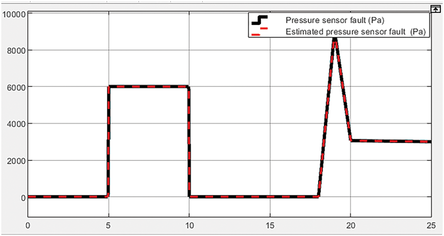
Figure 7: Pressure fault and its estimation without fault compensation

Figure 8: Piston position error without fault compensation

3.2 Simulation Results with Fault Compensation

Estimating pressure fault is performed using an unknown input observer model using the fault compensation technique. The effects of pressure fault (green line) have been minimized, as shown by the position feedback signal (blue line) compared to the reference signal (red line), as described in Fig. 9. Compared to the results without applying the fault compensation technique in Fig. 4, the quality of the position feedback signal is much better and more synchronous.

Figure 9: Comparison of the position feedback signal and demand signal with fault compensation case

Fig. 10 shows the similarity between the piston position response velocity and its estimation when applying for fault compensation. It is easy to see that the signal quality at the top and bottom has become much better. In addition, the pressure feedback signals at the two chambers under the influence of pressure fault also become more sinusoidal, as shown in Fig. 11.

Figure 10: The piston position response velocity with fault compensation case

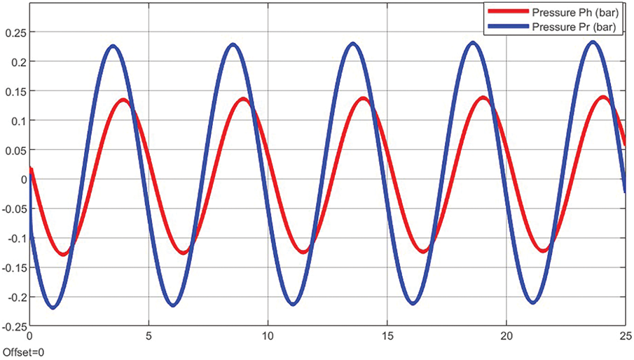
Figure 11: The pressure feedback signals with fault compensation

Fig. 12 shows the control error of Pload in the case of fault compensation. The process of fault compensation is shown in Fig. 13. The proposed fault compensation technique has significantly reduced the pressure sensor fault. The piston position error has been resolved thanks to the proposed pressure compensation process, as demonstrated in Fig. 14.

Figure 12: Residual of Pload with fault compensation

Figure 13: Pressure fault and its estimation with fault compensation

Figure 14: Piston position error with fault compensation

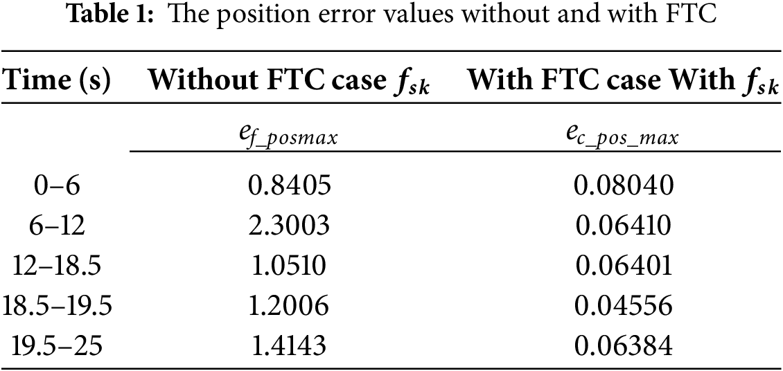
The simulation results show that, before applying the proposed fault compensation method, the position feedback signal of the piston deviates from the reference signal under the negative influence of pressure faults. The displacement velocity of the piston and the feedback pressure in the two chambers Ph and Pr are also adversely affected. Additionally, we have also identified the control error of Pload and the error emax. After applying the UIO fault estimation model, significant improvements have been made to these parameters. The position error in the case of a fault-free system, a faulty system, and when the system performs fault compensation are presented in Table 1.

3.3 Simulation Result with Uniform White Noise

To evaluate the stability of the proposed system, uniform white noise is applied in combination with the pressure sensor fault. The noise characteristics are illustrated in Fig. 15.

Figure 15: Uniform white noise

Figs. 16 and 17 present the simulation results of the system under the influence of environmental noise and pressure sensor faults, respectively. As observed in Fig. 16, when fault compensation is not applied, the response signal fails to meet the required performance, with an average error reaching up to 1.08265 mm. In contrast, with fault compensation, the response signal closely follows the reference signal, achieving an accuracy of up to 0.0212 mm.

Figure 16: System’s response to disturbances without fault compensation

Figure 17: System’s response to disturbances with fault compensation

For a clearer analysis of the estimated fault signal before and after applying fault compensation, the estimated fault values are illustrated in Figs. 18 and 19. In Fig. 19, it can be observed that the estimated fault has been effectively compensated.

Figure 18: Pressure fault and its estimation without fault compensation

Figure 19: Pressure fault and its estimation with fault compensation

Thus, even under the influence of noise in the presence of a pressure sensor fault, the compensation system ensures the response follows the reference signal.

3.4 Performance of Position Control Error

To evaluate the performance of the pressure fault compensation method, we apply a technique to assess the errors when the fault compensation technology is not applied and when it is applied, compared to the control error when there is no fault as follows:

The performance of position control error ηpos is compered between fault compensation cases and without fault compensation cases:

ηpos=|ef_posmax−ec_posmaxef_posmax|×100%(41)

where:

ec_posmax: The maximum position control error with fault compensation within a certain period of time.

ef_posmax: The maximum position control error without fault compensation within a certain period of time.

The results of the position control error performance, ηpos, are shown in Table 2. By employing the fault compensation method, our proposed system achieves a performance level exceeding 90%. Notably, when a pressure sensor fault occurs, the effectiveness of the pressure sensor fault compensation system becomes even more apparent.

4  Conclusion

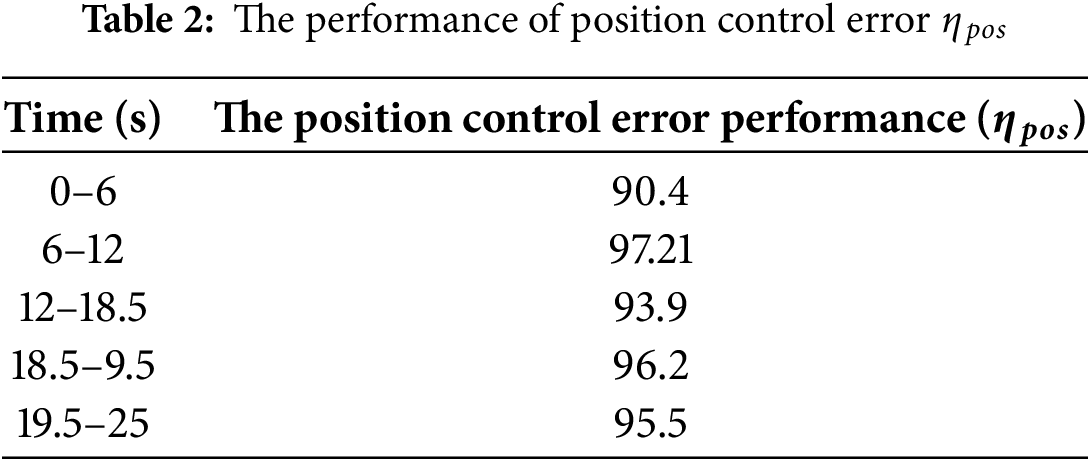
In aircraft control systems, multiple sensors can be used to ensure safety. In this paper, our objective was to control position through a pressure sensor. Furthermore, we have proposed a solution to minimize errors in the control process caused by sensor malfunctions. Here, we used fault-tolerant control technology, and a fault compensation method based on fault estimation technology. The fault estimation technology for pressure sensors was implemented through an unknown input observer estimator. Using the proposed approach, the position control error significantly improved when a pressure sensor fault occurred. Depending on the state of the fault’s impact, the fault compensation results varied. The fault compensation method ensures over 90% system performance, with its effectiveness becoming more evident under pressure sensor faults. Our proposed method faces challenges in real-time implementation due to the computational complexity of solving LMIs and sensitivity to measurement noise, which may affect fault estimation accuracy. Future research could focus on optimizing computational efficiency, enhancing robustness against uncertainties, and validating the approach on physical systems.

Acknowledgement: This work was supported by Nguyen Tat Thanh University, Ho Chi Minh City, Vietnam, provided with the facilities required to carry out this work.

Funding Statement: The authors received no specific funding for this study.

Author Contributions: The authors confirm contribution to the paper as follows: Conceptualization, Huy Q. Tran, Tan Nguyen Van, and Cheolkeun Ha; methodology, Huy Q. Tran and Tan Nguyen Van; formal analysis, Huy Q. Tran; investigation, Huy Q. Tran and Tan Nguyen Van; writing—original draft preparation, Huy Q. Tran and Tan Nguyen Van; writing—review and editing, Huy Q. Tran, Tan Nguyen Van, and Cheolkeun Ha. All authors reviewed the results and approved the final version of the manuscript.

Availability of Data and Materials: Not applicable.

Ethics Approval: Not applicable.

Conflicts of Interest: The authors declare no conflicts of interest to report regarding the present study.

References

1. He Y, Hu J, Chen X, Fei Y, Li E. Mechanical hydraulic control design of CNC equipment fault based on part quality. J Phys Conf Ser. 2021;2021(1):012014. doi:10.1088/1742-6596/2021/1/012014. [Google Scholar] [CrossRef]

2. Liu CJ. Analysis of CNC machine tool self-circulating hydraulic balance system. Acad J Eng Technol Sci. 2023;6(6). doi:10.25236/AJETS.2023.060606. [Google Scholar] [CrossRef]

3. Zhao YM, Bao YY, Zhang C, Xue F. Design and analysis of variable pressure control of aircraft hydraulic system. In: Proceedings of the 2020 5th International Conference on Mechanical, Control and Computer Engineering (ICMCCE). New York, NY, USA: IEEE; 2020. p. 815–9. doi:10.1109/ICMCCE51767.2020.00179. [Google Scholar] [CrossRef]

4. Yan T, Li P, Niu W. Research on modeling technology of aircraft hydraulic system based on AMESim. J Phys Conf Ser. 2022;2183(1):012007. doi:10.1088/1742-6596/2183/1/012007. [Google Scholar] [CrossRef]

5. Kosova F, Unver HO. A digital twin framework for aircraft hydraulic systems failure detection using machine learning techniques. Proc Inst Mech Eng Part C J Mech Eng Sci. 2023;237(7):1563–80. doi:10.1177/09544062221132697. [Google Scholar] [CrossRef]

6. Taherkhani A, Bayat F, Mobayen S, Bartoszewicz A. Dependable sensor fault reconstruction in air-path system of heavy-duty diesel engines. Sensors. 2021;21(23):7788. doi:10.3390/s21237788. [Google Scholar] [PubMed] [CrossRef]

7. Fadel MZ, Rabie MG, Youssef AM. Motion control of an aircraft electro-hydraulic servo actuator. IOP Conf Ser Mater Sci Eng. 2019;610:012073. doi:10.1088/1757-899X/610/1/012073. [Google Scholar] [CrossRef]

8. Churn PM, Maxwell CJ, Schofield N, Howe D, Powell DJ. Electro-hydraulic actuation of primary flight control surfaces. In: IEE Colloquium on All Electric Aircraft (Digest No. 1998/260); 1998 Jun 17; London, UK. doi:10.1049/ic:19980341. [Google Scholar] [CrossRef]

9. Shen K, Zhao D. Fault diagnosis for aircraft hydraulic systems via one-dimensional multichannel convolution neural network. Actuators. 2022;11(7):182. doi:10.3390/act11070182. [Google Scholar] [CrossRef]

10. Safavi S, Safavi MA, Hamid H, Fallah S. Multi-sensor fault detection, identification, isolation and health forecasting for autonomous vehicles. Sensors. 2021;21(7):2547. doi:10.3390/s21072547. [Google Scholar] [PubMed] [CrossRef]

11. Tran CD, Palacky P, Kuchar M, Brandstetter P, Dinh BH. Current and speed sensor fault diagnosis method applied to induction motor drive. IEEE Access. 2021;9:38660–72. doi:10.1109/ACCESS.2021.3064016. [Google Scholar] [CrossRef]

12. Byun YS, Kim BH, Jeong RG. Sensor fault detection and signal restoration in intelligent vehicles. Sensors. 2019;19(15):3306. doi:10.3390/s19153306. [Google Scholar] [PubMed] [CrossRef]

13. Huang S, Liao F, Teo RSH. Fault tolerant control of quadrotor based on sensor fault diagnosis and recovery information. Machines. 2022;10(11):1088. doi:10.3390/machines10111088. [Google Scholar] [CrossRef]

14. Zhong Y, Zhang W, Zhang Y, Zuo J, Zhan H. Sensor fault detection and diagnosis for an unmanned quadrotor helicopter. J Intell Robot Syst. 2019;96(3):555–72. doi:10.1007/s10846-019-01002-4. [Google Scholar] [CrossRef]

15. Zuo L, Yao L, Kang Y. UIO based sensor fault diagnosis and compensation for quadrotor UAV. In: Proceedings of the 2020 Chinese Control and Decision Conference (CCDC). New York, NY, USA: IEEE; 2020. p. 4052–57. doi:10.1109/CCDC49329.2020.9164802. [Google Scholar] [CrossRef]

16. Pazera M, Witczak M. A novel adaptive sensor fault estimation algorithm in robust fault diagnosis. Sensors. 2022;22(24):9638. doi:10.3390/s22249638. [Google Scholar] [PubMed] [CrossRef]

17. Van Nguyen T, Ha C. The actuator and sensor fault estimation using robust observer based reconstruction for mini motion package electro-hydraulic actuator. In: Intelligent computing methodologies. Cham, Switzerland: Springer; 2019. p. 244–56. doi:10.1007/978-3-030-26766-7_23. [Google Scholar] [CrossRef]

18. Gao S, Ma G, Guo Y, Zhang W. Fast actuator and sensor fault estimation based on adaptive unknown input observer. ISA Trans. 2022;129:305–23. doi:10.1016/j.isatra.2022.01.019. [Google Scholar] [PubMed] [CrossRef]

19. Van Nguyen T, Ha C. Sensor fault-tolerant control design for mini motion package electro-hydraulic actuator. Processes. 2019;7(2):89. doi:10.3390/pr7020089. [Google Scholar] [CrossRef]

20. Van Nguyen T, Ha C. Experimental study of sensor fault-tolerant control for an electro-hydraulic actuator based on a robust nonlinear observer. Energies. 2019;12(22):24337. doi:10.3390/en12224337. [Google Scholar] [CrossRef]

21. Chen H, Du D, Zhu D, Yang Y. UIO-based fault estimation and accommodation for nonlinear switched systems. Int J Control Autom Syst. 2019;17(2):435–44. doi:10.1007/s12555-018-0314-4. [Google Scholar] [CrossRef]

22. Gao S, Zhang W, Zhang Z. H−/L∞ UIO-based actuator and sensor fault diagnosis design in the finite frequency domain for discrete-time Lipschitz nonlinear systems. IET Control Theory Appl. 2022;16(14):1458–73. doi:10.1049/cth2.12323. [Google Scholar] [CrossRef]

23. Jiang T, Li T, Wang L. Based on UIO fault estimation for Markov jump systems. In: Proceedings of the 2017 Eighth International Conference on Intelligent Control and Information Processing (ICICIP). New York, NY, USA: IEEE; 2017. p. 74–8. doi:10.1109/ICICIP.2017.8113920. [Google Scholar] [CrossRef]

24. Liu Y, Wang ZD, Zhou DH. UIO-based fault estimation for a class of time-varying systems with event-triggered transmissions. IFAC-PapersOnLine. 2018;51(24):46–51. doi:10.1016/j.ifacol.2018.09.527. [Google Scholar] [CrossRef]

25. Sheydaeian Arani AA, Shoorehdeli MA, Moarefianpour A, Teshnehlab M. Fault estimation based on ensemble unscented Kalman filter for a class of nonlinear systems with multiplicative fault. Int J Syst Sci. 2021;52(10):2082–99. doi:10.1080/00207721.2021.1876959. [Google Scholar] [CrossRef]

26. Wang M, Liang T. Adaptive Kalman filtering for sensor fault estimation and isolation of satellite attitude control based on descriptor systems. Trans Inst Meas Control. 2019;41(6):1686–98. doi:10.1177/0142331218787605. [Google Scholar] [CrossRef]

27. Liu Z-X, Wang Z-Y, Wang Y, Ji Z-C. Optimal zonotopic kalman filter-based state estimation and fault-diagnosis algorithm for linear discrete-time system with time delay. Comput Mater Contin. 2022;79(4):4651–68. doi:10.32604/cmc.2022.054960. [Google Scholar] [CrossRef]

28. Ghanbarpour K, Bayat F, Jalilvand A. An MPC-based fault tolerant control of wind turbines in the presence of simultaneous sensor and actuator faults. Comput Electr Eng. 2025;122(4):109931. doi:10.1016/j.compeleceng.2024.109931. [Google Scholar] [CrossRef]