CMS-YOLO: An Automated Multi-Category Brain Tumor Detection Algorithm Based on Improved YOLOv10s

1  Introduction

Brain tumors are diseases with a high mortality rate that develop as a result of cell-specific lesions in brain tissue [1]. According to the latest statistics, the number of deaths caused by brain tumors has increased by 300% in the past three decades. In 2022, 248,300 deaths and 321,500 new incidents of malignant brain tumors occurred worldwide [2]. In the same year, the number of brain tumor deaths in China was 56,600, while the number of incident cases was 87,500. The mortality rates among males and females were 4.38 and 3.63 per 100,000, respectively, while the incidence rates were 5.88 and 6.53 per 100,000, respectively [3]. The large morbidity and mortality data reflect the diversity and complexity of brain tumor types. Common brain tumors include meningioma, pituitary tumors, and nerve sheath tumors. According to the factors of tissue origin, cell morphology, and biological characteristics, brain tumors can be classified as either benign or malignant. Most benign brain tumors are small in size and grow slowly. When they are in key functional areas, they can compress surrounding tissues such as blood vessels and nerves at an early stage. Additionally, some of these tumors exhibit invasive characteristics. Malignant tumors not only compress the surrounding tissues but may also spread through the cerebrospinal fluid and other ways to affect the function of other bodily components, inducing a series of complications and endangering the lives of patients [4]. Consequently, the prompt discovery and accurate positioning of the lesion region play a vital role in the subsequent diagnosis and treatment of brain tumors. Among the traditional brain tumor detection methods, Magnetic Resonance Imaging (MRI) can help identify the presence, location, and size of brain tumors due to its high resolution and soft tissue sensitivity, which allows for the detailed visualization of subtle changes in brain structure [5]. However, MRI images struggle to accurately distinguish brain tumors that resemble surrounding brain tissue. Additionally, its diagnostic accuracy relies on medical expertise and physicians’ experience, and the time-intensive analysis process can easily result in misdiagnosis or missed detection.

Artificial intelligence (AI) methods are demonstrating significant potential in the medical field and are profoundly changing the traditional medical model. For example, the “Chest CT Intelligent 4D Imaging System” developed by Zhejiang Provincial People’s Hospital has led the way in realizing the practical application of AI technology in medical imaging in China. It has significantly improved the efficiency and accuracy of lung nodule detection [6]. In terms of medical system construction and intelligent diagnosis, the AI hospital established by Tsinghua University will initially set up an AI hospital system. In the future, it will construct an ecological closed loop of “AI + Medicine + Education + Research”. In addition, the internal testing system of “Bauhinia AI Doctor” developed by the team has been officially launched. There are 42 AI doctors from various departments in the system, covering over 300 types of diseases. It helps doctors reduce their workload and improve work efficiency, thereby contributing to the improvement of diagnosis and treatment quality and the reduction of the misdiagnosis rate [7]. The application of these AI systems also integrates the latest medical research, clinical guidelines, and individual patient data to provide doctors with evidence-based medical support to assist complex treatment decisions [8]. Consequently, the utilization of sophisticated AI methods to facilitate the rapid and precise detection of brain tumors is of significant research value.

Over recent years, Deep Learning (DL) techniques have made breakthroughs in the field of medical image processing, particularly in lesion region segmentation [9,10], disease classification [11,12], and disease detection [13–15]. These technologies allow the automatic extraction of features and information from image data, thereby assisting physicians in clinical diagnosis. This not only alleviates the work burden of physicians but also substantially enhances the accuracy and efficiency of medical image analysis [16]. DL methods can automatically extract features related to brain tumors by analyzing brain MRI images. Therefore, key information such as the shape and size of the brain tumor is obtained. A DL network architecture can be constructed using the extracted features, which allows the precise identification of brain tumors in unknown MRI images and the further classification of the type of brain tumor [17]. The implementation of brain tumor diagnosis tasks based on DL methods can be divided into segmentation, classification, and detection. In previous studies, Tian et al. [18] proposed a fully automatic multi-tasking brain tumor segmentation network based on multi-modal feature reorganization and scale crossing attention mechanism. This framework not only takes into full consideration the complementary and shared information between modalities but also automatically learns the attention weights of each modality to acquire more targeted lesion features, thus improving the accuracy of brain tumor segmentation. Ghazouani et al. [19] utilized a three-dimensional enhanced local self-attention (3D ELSA) transformer block to enhance the local feature extraction. They proposed a three-dimensional (3D) brain tumor image segmentation network based on an ELSA Swin transformer for the first time, which achieved a Dice score of 89.77% and an average Hausdorff distance of 8.99 mm. Nevertheless, the stacking of multiple modules may deteriorate the model’s interpretability and cause it to fail to meet the actual scenarios. Li et al. [20] inserted multilevel residual blocks between the encoder and decoder of the U-Net network and incorporated the channel attention mechanism. As a result, they put forward a multi-scale deep residual convolutional neural network, which is designed to enhance the precision of brain tumor segmentation. The problem of brain tumor segmentation in three-dimensional Magnetic Resonance Imaging (3D MRI) images was solved. However, the number of samples that could be used for brain tumor segmentation was small at that time, and the model generalization ability was not verified.

In order to solve the problems of insufficient feature extraction ability of traditional models and weak model generalization ability due to the variability of the dataset, Wu et al. [21] combined the federated learning framework, improved residual network, and convolutional attention module to propose the FL-CBAM-DIPC-ResNet model for brain tumor classification. By implementing a lightweight network MobileNetV2 for feature extraction, a single model dedicated to the brain tumors’ hierarchical classification was suggested by Sankar et al. [22]. This was aimed at overcoming the problem of classifying various grades of brain tumors due to their differences in size, shape, and position. It achieved classification accuracies of 99.87% in binary classification and 99.38% in multi-class classification, respectively. Nassar et al. [23] introduced an effective method for classifying brain tumors based on a hybrid mechanism of majority voting. The method precisely identifies three categories of brain tumors by applying a majority voting operation to the outputs of five pre-trained models. However, the brain tumor data samples used for training are small in number, and a sample imbalance problem exists. Moreover, the model structure and decision-making process are relatively complex, making it difficult to intuitively explain how the model makes decisions, which is not conducive to the doctors’ understanding of the basis of the model’s judgment.

Utilizing DL techniques for the segmentation and classification of brain MRI images enables the rapid identification of brain lesions within the images. This aids doctors in formulating more precise diagnoses and improves diagnostic efficiency and correctness for medical practitioners. Nevertheless, neither of these two tasks is capable of precisely identifying the location of brain tumors. On the contrary, the detection task is capable of not only identifying the presence of a brain tumor in the image but also accurately pinpointing its location, thereby enabling the classification and localization of brain tumors. In a related study of brain tumor detection using traditional Convolutional Neural Network (CNN) and Transfer Learning (TL) methods, Ge et al. [24] proposed a novel unsupervised learning dual-branching framework, Double-SimCLR, which can simultaneously process MRI and computed tomography (CT) images to achieve multimodal feature fusion and solve the low diagnostic accuracy associated with single modality images. The method obtained 92.46% accuracy and 93.06% F1-score. Hossain et al. [25] considered the detection and classification of multi-category brain tumors and proposed the use of TL model integration to obtain the integrated model IVX16, and used the Local Interpretable Modeling Algorithm (LIME) to verify the effectiveness of the proposed model. The experimental results show that the classification accuracy of the integrated model is 96.94%, indicating that the method can effectively avoid the overfitting problem. However, developing integrated models with TL methods usually requires training multiple base models, which can substantially increase training time. Gürsoy et al. [26] proposed a fusion deep learning model Brain-GCN-Net by combining Graph Neural Networks (GNN) with CNN. It can capture global and local information, and more comprehensively analyze the intricate features within brain tumor images, achieving a classification accuracy of 93.68%. However, this method has poor performance in detecting small tumors and brain tumors that are similar to the surrounding tissue.

In addition to CNNs and TL methods, object detection algorithms, through end-to-end training, can directly localize and classify brain tumors, providing a new approach to the brain tumor detection task. Kang et al. [27] proposed a Reparametrized Convolutional YOLO architecture, RCS-YOLO, which extracts richer features and significantly improves the preciseness and rapidity of the model in detecting brain tumors. This is achieved by designing a Reparametrized convolutional shuffle (RCS) module and a practical one-shot aggregation module (RCS-OSA). As a result, the detection time is significantly reduced. Nevertheless, it does not work well when dealing with complex background images. Chen et al. [28] proposed the YOLO-NeuroBoost model for brain tumor detection, which combines the YOLOv8 network with the dynamic convolutional KernelWarehouse, Convolutional Block Attention Module (CBAM) technique. Moreover, instead of the Complete-IoU (CIoU) loss, it applies the Inner-Generalized IoU (Inner-GIoU) loss function to calculate the bounding box loss. However, the detection effect is inferior for intricate backgrounds, such as those with high noise and low contrast. Costa Nascimento et al. [29] proposed a novel generative AI approach based on the concept of synthetic computing cells combined with YOLO detection, which can detect, segment, and classify brain tumors. The experimental results demonstrated that this method achieves an accuracy of more than 95% in region detection, segmentation, and classification of brain tumors. However, the method is ineffective in the complex case where the brain tumor is located at the edge of the image. Muksimova et al. [30] proposed an entirely novel brain tumor detection method, which integrates the enhanced spatial attention (ESA) layer into the YOLOv5m model to help enhance the model’s ability to distinguish brain tumors. Experimental results show that the method obtains 92% precision and 87.8% recall, respectively, highlighting the transformative potential of deep learning in the medical field. However, the dataset used for the model is relatively homogeneous and the model’s generalization ability is poor.

Currently, most brain tumor detection methods, whether traditional CNN methods, TL methods, or target detection algorithm applications, have their limitations. In particular, detecting brain tumors with varying shapes and sizes faces challenges, including high false positive and false negative rates, and poor real-time performance. Additionally, some brain tumors are similar to the characteristics of the surrounding tissues or other lesions, which leads to increased difficulty in detection. YOLOv10 [31] retains the advantages of the previous You Only Look Once (YOLO) model, suggested the training strategy without Non-Maximum Suppression (NMS), and improved the driven module. This improvement significantly enhanced the model’s comprehensive capacity in terms of effectiveness and performance, overcoming the limitations of detection speed and accuracy in identifying brain tumors. Therefore, this paper proposes a YOLOv10s-based improved model, CMS-YOLO, for the detection of brain tumors. The model can more effectively extract features of brain tumors in the presence of complex backgrounds, thanks to the improvements in feature extraction and fusion. Furthermore, the proposed approach not only enhances the detection speed and precision but also enables real-time detection of various brain tumor types. The model helps doctors identify brain tumors quickly and accurately, thereby improving diagnostic accuracy and efficiency.

The main contributions of this paper are as follows:

•   Introducing Convolutional Medical UNet extended block (CMUNeXt Block) in the backbone of the YOLOv10s model innovatively proposes the C2f_CMUNeXtB module to enhance the model’s extraction of global context information.

•   Add the Multi-scale Attention Aggregation (MSAA) module to the neck to enable the model to achieve multi-scale fusion of brain tumor features, thereby enhancing the model’s capability to handle intricate backgrounds and reduce background interference.

•   By replacing the conventional bounding box loss with the Shape-IoU loss function, the model is enabled to prioritize the size and shape of the bounding box, thereby enhancing the accuracy of bounding box regression and the detection of small tumors.

The paper is organized as follows: Section 2 clarifies the dataset and evaluation metrics utilized in this research, and details the data processing methods. Section 3 describes the framework of the proposed methodology. Section 4 elaborates on the parameter settings for model training, describes the training process of the proposed model, and presents a comparison with state-of-the-art algorithms. Section 5 provides a detailed overview of the research conclusions, and the limitations of this study, and examines possible directions for future investigation.

2  Materials and Methods

In this section, we will describe the dataset used in this study, the data processing methods employed, and the various evaluation metrics used to assess the model’s performance.

2.1 Data Sources

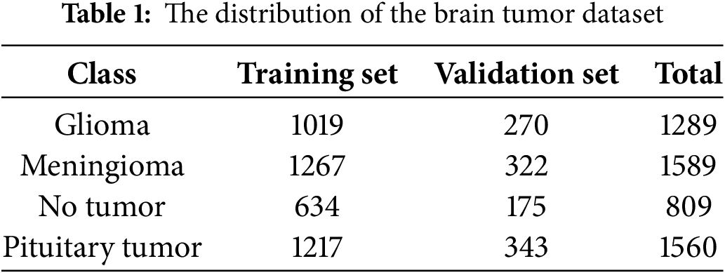
The “MRI for Brain Tumor with Bounding Boxes” dataset was acquired from Kaggle to validate the performance and effectiveness of the model. The dataset acquisition link is as follows: https://www.kaggle.com/datasets/ahmedsorour1/mri-for-brain-tumor-with-bounding-boxes (accessed on 20 June 2025). The dataset comprises 5249 axial, coronal, and sagittal brain MRI images with detailed annotations of tumor types, locations, and sizes, which are often used for the automated detection and classification of brain tumors for research. Comprising three types of brain tumor images: glioma (1289 images), meningioma (1589 images), and pituitary tumor (1560 images), along with normal brain images (809 images). Additionally, these images were partitioned into a training set including 4737 images and a validation set containing 512 images. Fig. 1 displays the sample diagram of the dataset.

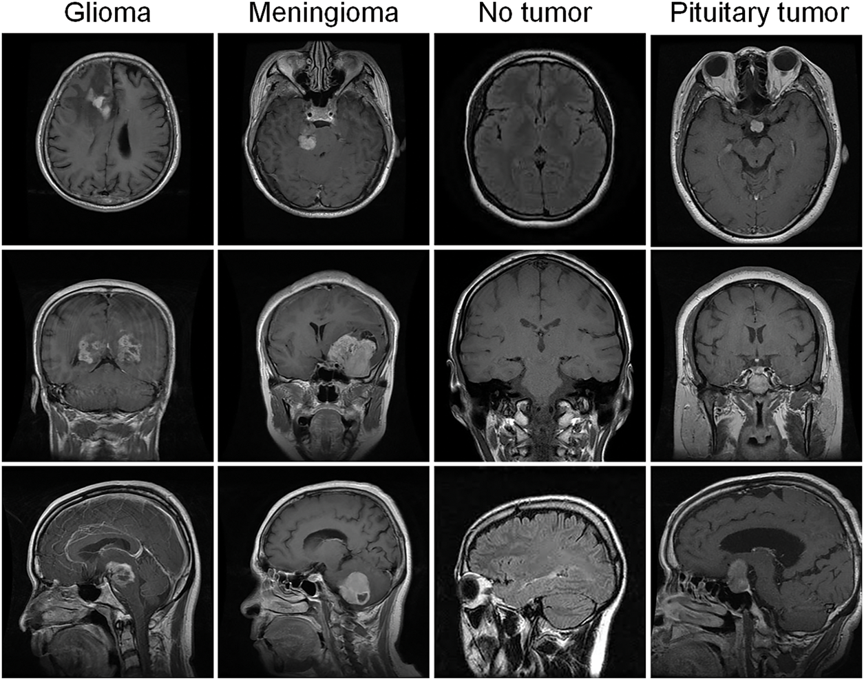
Figure 1: Sample plot of the dataset

2.2 Data Processing

In this study, the dataset was processed using data screening, data normalization, and data division to enhance the quality and diversity of samples and improve the model’s capability to handle unknown data.

(1)   Data screening: The dataset is screened to ensure its quality and annotation completeness.

(2)   Normalization: There are great differences among features in the dataset, which can impact the model training. Therefore, before training the model, it is crucial to normalize the data to adjust the feature values of various dimensions to similar ranges. This process ensures the model’s stability during gradient updating in training and improves the model’s performance. The Min-Max normalization method is adopted, and its expression is shown in Eq. (1):

xnorm=x−xminxmax−xmin(1)

In this context, xnorm represents the normalized data, x indicates the initial data, xmax and xmin indicate the maximum and minimum values in the dataset, respectively.

(3)   Data division: Although the initial dataset was split into a training set and a validation set, the number of samples in the validation set is too small to demonstrate how the model performs with unknown data. There is also a risk of insufficient generalization ability and overfitting. Therefore, considering the model’s training needs, the dataset is divided into an 8:2 ratio. Specifically, 80% of the data is designated for the training set, while 20% is allocated for the validation set.

Following the data processing described above, two images without annotations were excluded, and the final training set consists of 4137 images, while the validation set contains 1110 images. Table 1 shows the distribution of the brain tumor dataset.

2.3 Evaluation Metrics

Utilizing metrics such as a confusion matrix, precision, recall, F1−score and mean average precision (mAP) for assessing the effectiveness of the suggested brain tumor detection approach.

The confusion matrix, also known as the classification matrix, serves to assess the model’s classification capabilities, clarify the relationship between the actual labels and the predicted outcomes, and help understand the model’s performance across various categories. For multi-categorization problems, each cell in the confusion matrix represents the number of samples that are actually in one category but are predicted to be in another. After normalizing the confusion matrix, each cell represents the proportion of samples that are actually of one class but predicted to be of another class. In this way, the classification accuracy can be obtained intuitively to evaluate the model’s performance.

Precision (P) denotes the ratio of true positive samples to all the samples predicted positive by the model. It aims to evaluate the model’s ability to identify brain tumors accurately. The higher the precision, the lower the false positive rate. Recall (R) refers to the portion of true positive samples that the model accurately recognizes among the overall amount of actual positive samples. It is used to measure the comprehensiveness of the model in detecting brain tumors. The higher the recall, the lower the false negative rate. The F1−score indicates the harmonic average of precision and recall, which takes both P and R into comprehensive consideration and is used to balance the relationship between them. The calculation formulas of these three indicators are shown in Eqs. (2)–(4):

P=TPTP+FP(2)

R=TPTP+FN(3)

F1-score=2×(P×R)P+R(4)

In the above formula, TP (True Positive) denotes the number of samples that are correctly predicted as positive and are positive; FP (False Positive) is used to reflect the false detection situation of the model, which denotes the number of samples that are forecasted as positive but in fact negative. FN (False Negative) reflects the miss-detection situation of the model, which represents the total amount of samples that are predicted to be negative but are truly positive.

The precision-recall (P-R) curve is plotted with recall on the horizontal axis and precision on the vertical axis, providing a graphical evaluation of model performance across varying threshold settings. Average Precision (AP) is defined as the area under the P-R curve, where higher values of AP indicate better average precision of the model. The calculation of AP is shown in Eq. (5):

AP=∫01P(R)dR(5)

The mean Average Precision (mAP) is obtained by taking the average of the AP values throughout all categories, as illustrated in Eq. (6). This metric assesses the algorithm’s average performance within all categories. mAP50 is defined as the mAP value when the Intersection over Union (IoU) threshold has been set at 0.5. mAP50-95 represents the mAP when the IoU threshold ranges from [0.5, 0.95].

mAP=∑i=1NAPiN(6)

where, N refers to the number of categories.

3  Methodology

In this section, we will analyze the overall structure of the model and the various methods employed within it.

3.1 Overall Model Structure

Figs. 2 and 3 illustrate the simplified structural diagram of this study and the basic framework of the model proposed in this paper. Moreover, Fig. 3 further illustrates the detailed diagrams of each part presented in Fig. 2. Fig. 4 presents the internal structure of each module in the model. This model is further improved using the YOLOv10s algorithm, comprising three primary parts: the Backbone, Neck, and Head. These different parts are responsible for feature extraction, feature fusion, and target classification and localization, respectively.

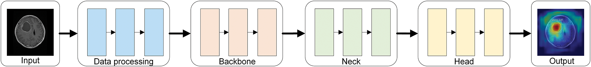
Figure 2: Simplified diagram of the research methodology

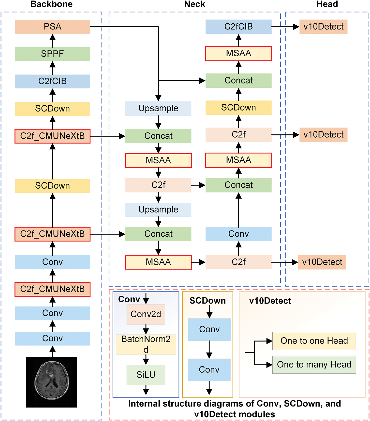
Figure 3: The overall architecture of the CMS-YOLO model

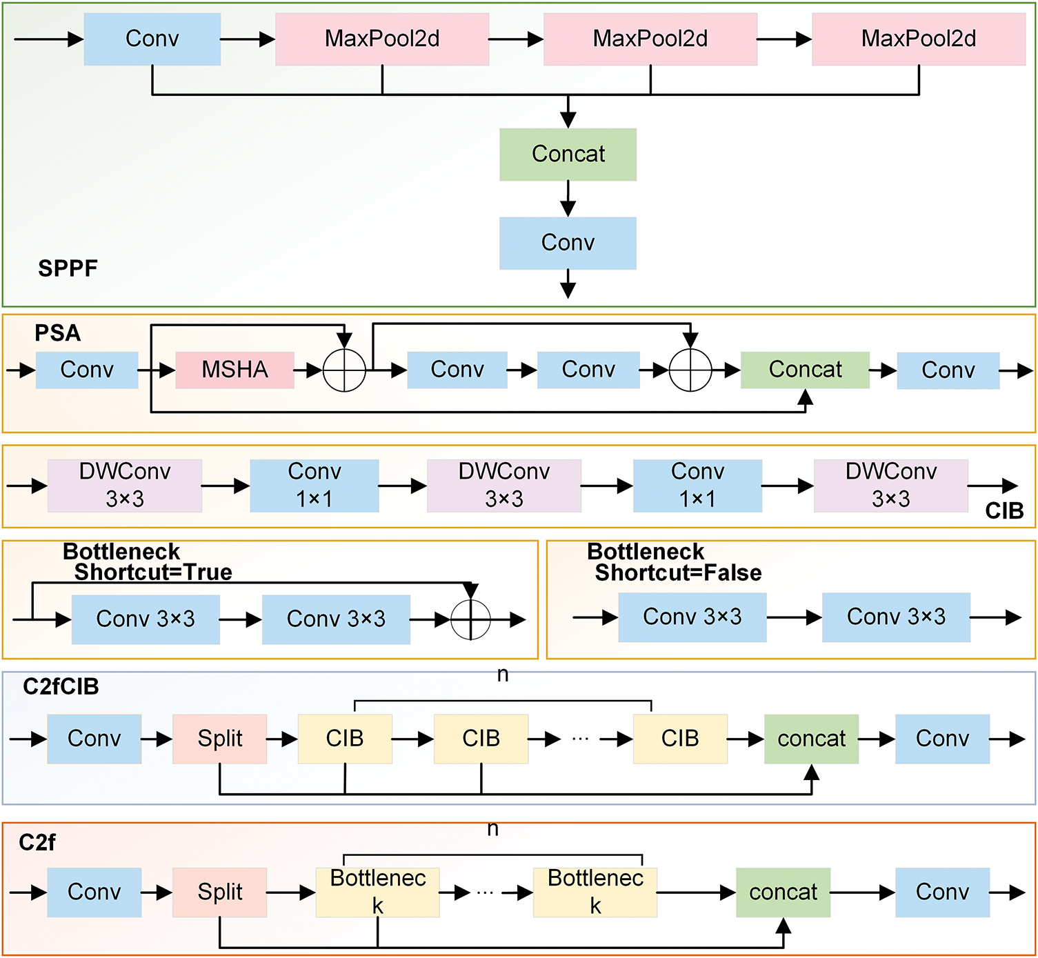
Figure 4: The internal structure diagram of each module

The CMUNeXt Block is introduced in the CSP Bottleneck with 2 Convolutions (C2f) at the Backbone stage, and the C2f_CMUNeXtB module is creatively suggested. The CMUNeXt Block adopts large kernel separable convolution to extract global information, addressing the network’s challenge of capturing global information by fully extracting and mixing the long-range spatial location information in brain tumor images with the fewest possible parameters.

In the Neck stage, the MSAA module is introduced before the predictive feature layer to conduct refined processing on the features obtained through concatenation. This helps address the deficiencies in feature extraction and fusion, reduces background interference, and enhances the algorithm’s capacity to process intricate backgrounds.

During the Head stage, the Shape-IoU loss function is employed, enabling the model to learn the target’s shape characteristics more accurately by focusing on the bounding box’s size and shape. This process enables the model to focus on the core region of the brain tumor, thereby not only improving its anti-interference ability but also enhancing its capacity to detect brain tumors in intricate scenarios and its robustness.

3.2 C2f_CMUNeXtB Module

In CMUNeXt Block [32], the conventional convolution is replaced with Depthwise Convolution (DW Conv) and Pointwise Convolution (PW Conv). The CMUNeXt Block first adopts the DW Conv with a large kernel to extract the global information of each channel. After that, two PW convolutions are employed to realize that the number of channels initially increases and subsequently decreases, thereby establishing an inverted bottleneck structure. This structure enables the comprehensive combination of spatial and channel information, realizing the efficient extraction of global context information. The overall process is represented as Eqs. (7)–(9):

f1=BN(δ(DWConv(a)))+a(7)

f2=BN(δ(PWConv(f1)))(8)

Y=BN(δ(PWConv(f2)))(9)

where a is the output of the previous layer, Y is the output feature map of CMUNeXt Block, δ is the GELU activation function layer, and BN represents the Batch Normalization layer. DWConv is the DW convolution, and PWConv is the PW convolution. Fig. 5 illustrates the structure of the C2f_CMUNeXtB module.

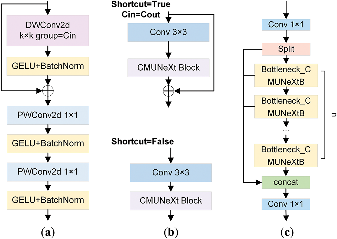
Figure 5: The diagrammatic illustration of the C2f_CMUNeXtB module and its related components. (a) illustrates the structure of the CMUNeXt Block. (b) displays the overall layout of the Bottleneck_CMUNeXtB module. (c) exhibits the structural diagram of the C2f_CMUNeXtB module

As an essential part of the YOLOv10s network, the C2f module enables the network to handle complex brain tumor MRI image features by extracting and transforming features through operations of feature transformation and fusion. The C2f_CMUNeXtB module is proposed by introducing the CMUNeXt Block to improve the Bottleneck structure, which reduces the number of network parameters and the computation while enhancing the model’s capacity to extract the global context information from brain tumor MRI images and enriches the expression of features.

3.3 MSAA Module

The MSAA module is recognized for its capacity to fuse features at varying scales and for its exceptional capability to handle complex backgrounds [33]. On the other hand, the YOLOv10s model is inadequate at extracting fine details from complex scenes, resulting in a decrease in detection performance. Given this, the MSAA module is added to compensate for the insufficient feature extraction and information fusion inside cross-layer spliced features.

MSAA aims to enhance the model’s capability to identify and comprehend image details by combining various scale features. Fig. 6 presents the structure of the MSAA module. It consists of two branches: spatial and channel. In the spatial refinement path, the number of channels is first reduced through a 1 × 1 convolution kernel, and then the results of three convolutions with different sizes are summed up. Finally, a series of spatial feature aggregation operations are carried out. Through the above operations, multi-scale information fusion is achieved in the spatial dimension. The extraction and fusion process of features in the spatial path can be expressed as Eqs. (10) and (11):

Y1=f3(f(x1))⊕f5(f(x1))⊕f7(f(x1))(10)

Y2=f(Y1⊗σ(f7(Pmax(Y1))))(11)

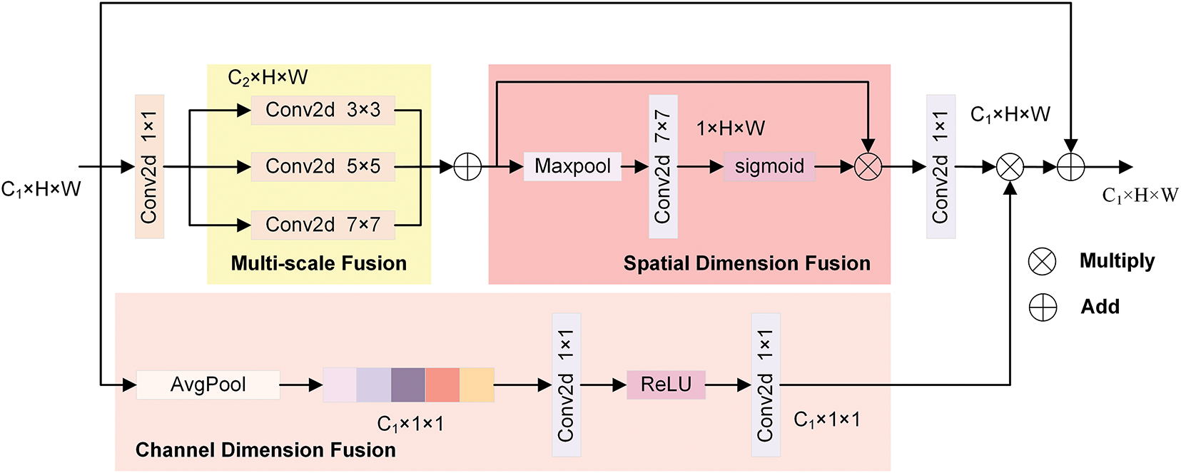
Figure 6: The structural chart of the MSAA module

where ⊕ and ⊗ stand for denotes pixel-by-pixel summation and multiplication, respectively. Y1 is the multi-scale fusion output, Y2 is the spatial dimension fusion output, and x1 is the input feature, f denotes 1 × 1 convolution operation, f3, f5 and f7 denotes convolution layers with kernel dimensions of 3 × 3, 5 × 5 and 7 × 7, respectively, Pmax is the maximum pooling, and σ is the Sigmoid activation function. During this process, leveraging spatial refinement path to perform a weighted integration of spatial features in the feature map.

On the channel aggregation path, the feature map dimensionality is first reduced using average pooling. Subsequently, the channel attention maps are generated using convolution and Rectified Linear Unit (ReLU) activation functions, thereby enhancing the features of the designated channels. The aggregation on the channel path is shown in Eq. (12):

Y3=f(ε(f(Pavg(x1))))(12)

where Y3 is the channel dimension fusion output feature map, Pavg is the average pooling, and ε is the ReLU activation function. After multipath processing, the output feature maps of the channel aggregation paths and the output feature maps of the spatial refinement branches are fused by multiplication, and the overall calculation of the MSAA module is shown in Eq. (13):

Y=x⊕(Y2⊗Y3)(13)

By utilizing the MSAA module to fuse features at different scales, the feature characterization ability is enhanced, and the background interference in MRI images is reduced. Thus, the model’s capacity to recognize tumors of various sizes is significantly enhanced, as is its performance in detecting brain tumors.

3.4 Shape-IoU Loss Function

The target detection loss consists of classification loss (lcls) and bounding box regression loss (lreg). lcls is used to evaluate the difference between the predicted and actual categories. Meanwhile, lreg is utilized to measure the positional discrepancy between the predicted and Ground Truth (GT) boxes. In YOLOv10s, the lcls is computed using the binary cross-entropy loss (BCELoss) function, which helps address a situation of class imbalance in the dataset. The lreg is calculated using the Complete-IoU (CIoU) loss. However, the lreg based on IoU usually only focuses on the geometric correlation between the GT box and the anchor box. This approach calculates the loss by considering the relative positions and forms of the bounding boxes while neglecting the impact of intrinsic attributes that characterize the bounding boxes themselves. This results in an inability to adaptively adjust to different detectors and detection tasks in practical applications and also leads to poor model generalization ability. This paper considers replacing the CIoU method with Shape-IoU [34] for calculating the lreg. Fig. 7 illustrates the description of Shape-IoU. The formula for the computation of the Shape-IoU loss function follows Eqs. (14)–(19):

IoU=|B∩Bgt||B∪Bgt|(14)

ww=2×(wgt)s(wgt)s+(hgt)s(15)

hh=2×(hgt)s(wgt)s+(hgt)s(16)

Dshape=hh×(xc−xcgt)2c2+ww×(yc−ycgt)2c2(17)

Ωshape=∑t=w,h(1−e−wt)θ,θ=4(18)

LShape-IoU=1−IoU+Dshape+0.5×Ωshape(19)

where Bgt and B denote the GT box and the prediction box, respectively. s is the scale factor, which is related to the proportion of targets in the dataset. wgt and w are the widths of the GT box and the Anchor box, respectively, hgt and h are the heights of the GT box and the Anchor box, respectively, (xcgt,ycgt) and (xc,yc) are the center coordinates of the GT box and the Anchor box, respectively. The value of ww and hh, which represent the horizontal and vertical weight coefficients, respectively, are contingent upon the geometry of the GT box. The value of θ determines the importance of the shape cost, and the value of this parameter is in the range of 2 to 6.

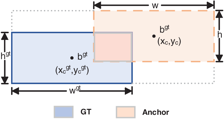
Figure 7: The diagram of the GT Box and Anchor Box in Shape-IoU

Shape-IoU raises the precision of regression with bounding boxes by concentrating on their size and shape during the loss calculation. This method significantly increases the accuracy and efficacy of tumor detection in MRI images by reducing background interference.

4  Experiments and Results Analysis

Following a description of the dataset used and the related techniques, this section focuses on analyzing the experimental results. Specifically, we will elaborate on the details of the experimental setup and analyze the experimental results obtained from the model training. In addition, ablation experiments are conducted to analyze the role of each component in the model thoroughly, and the visualization methodology adopted in this study is introduced to present the research results intuitively.

4.1 Experimental Setting

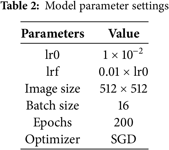
This study was conducted on a computing platform equipped with a Windows 11 operating system, an Intel 14600k processor, and an RTX 4060 Ti 24 G ×1 graphics card. The code used for the experiments was in the Python programming language, using the PyTorch deep learning framework. The model training parameters are presented in Table 2, and the model is trained using the Stochastic Gradient Descent (SGD) optimization algorithm with an output image size of 512 × 512. The initial learning rate (lr0) during training was 1 × 10−2, and the final learning rate (lrf) was 0.01 times the lr0. For model training, the Batch size was set to 16, while the number for training iterations (Epochs) was 200. Model training is conducted on large-scale dataset rows using pre-trained weight parameters to optimize the model’s performance. These settings ensure that key features can be effectively extracted from the input images during model training while also taking into account the high demand for computational resources during the training process.

4.2 Experimental Results

4.2.1 Compare with the Baseline Model

The experiment was conducted using the previously mentioned parameter settings, with YOLOv10s as the Baseline model. Fig. 8 displays the normalized confusion matrices of the Baseline model and the CMS-YOLO model. The detection results of the Baseline model and the CMS-YOLO model for various tumor types are presented in Tables 3 and 4, respectively. Fig. 9 shows the F1−score, mAP50 and mAP50-95 of the baseline model and the CMS-YOLO model on various types of brain tumors. It can be observed that the Baseline model achieves classification accuracies of 89.0% for gliomas, 97.0% for meningiomas, 99.0% for healthy MRI images, and 92.0% for pituitary tumors. In contrast, the CMS-YOLO model’s classification accuracy is 93.00%, 99.00%, 98.00%, and 93.00%, respectively. Compared with the Baseline model, the detection accuracy of the CMS-YOLO model for tumor-free MRI images has decreased by 1%, which has a relatively small impact on the overall evaluation of the model. On the other hand, the detection accuracy for glioma has increased by 4%, and the detection accuracies for both meningioma and pituitary tumors have increased by 1%. These results indicate that the improvement of the network structure by the CMS-YOLO model significantly improves the ability to capture the subtle features of brain MRI images, offering superior stability and reliability, and enabling more precise detection of brain tumors.

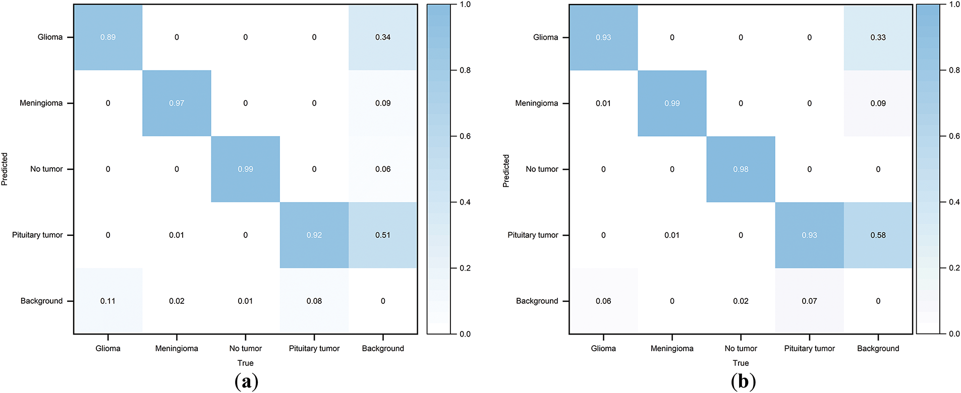
Figure 8: Normalized confusion matrix. (a) The normalized confusion matrix of the Baseline model. (b) The normalized confusion matrix of the CMS-YOLO model

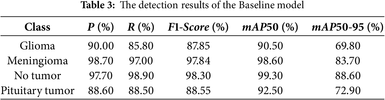
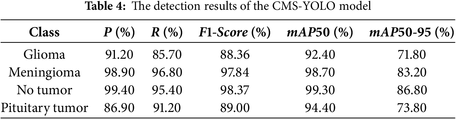
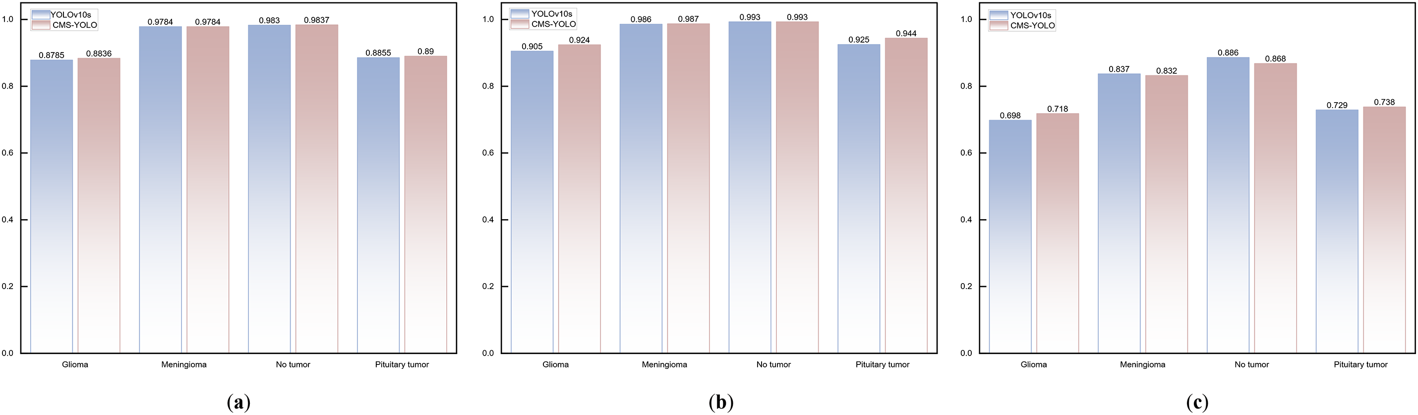
Figure 9: The comparison results of the Baseline model and CMS-YOLO for various brain tumor detection. (a) The comparison results of the F1-score between the Baseline Model and CMS-YOLO in different brain tumors. (b) The comparison results of the mAP50 between the Baseline Model and CMS-YOLO in different brain tumors. (c) The comparison results of the mAP50-95 between the Baseline Model and CMS-YOLO in different brain tumors

Figs. 10 and 11 illustrate the training processes of the Baseline and the CMS-YOLO models, and Fig. 10 shows the loss changes of the two models. After 200 Epochs, the detection performance of both models is steadily improving. On all three losses, the CMS-YOLO model has lower losses than the Baseline model, indicating that the method’s performance has been significantly improved. It can better fit the training data and has an increased capacity for generation.

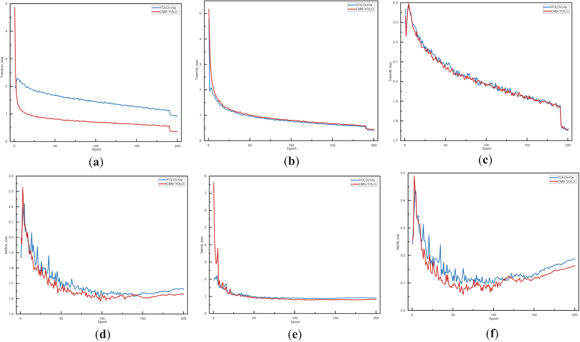
Figure 10: The loss variation of the YOLOv10s and the CMS-YOLO model. (a) The bounding box loss of YOLOv10s and the CMS-YOLO model on the training set. (b) The classification loss of YOLOv10s and the CMS-YOLO model on the training set. (c) The distribution focal loss of YOLOv10s and the CMS-YOLO model on the training set. (d) The bounding box loss of YOLOv10s and the CMS-YOLO model on the validation set. (e) The classification loss of YOLOv10s and the CMS-YOLO model on the validation set. (f) The distribution focal loss of YOLOv10s and the CMS-YOLO model on the validation set

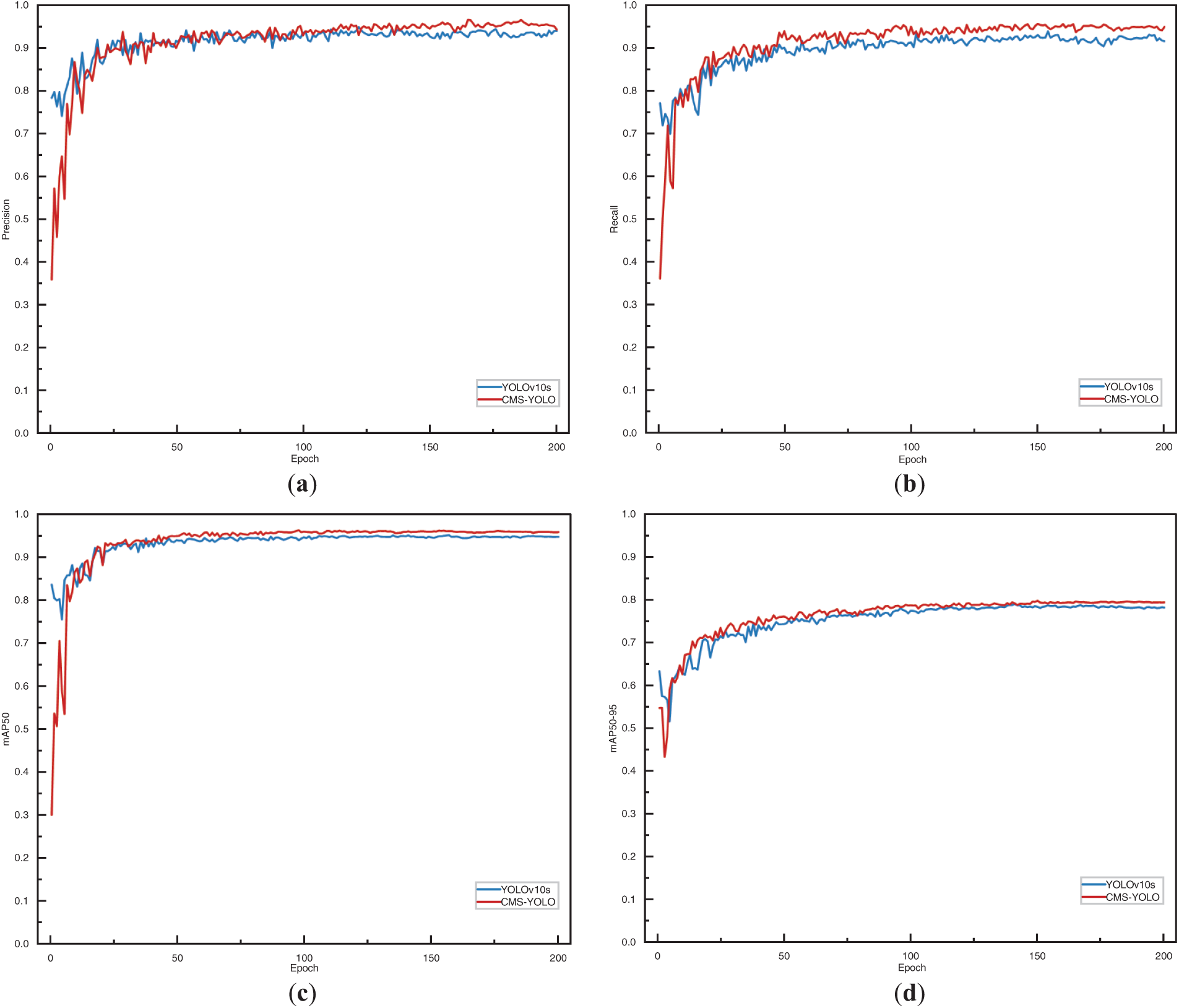
Figure 11: The performance metrics of the YOLOv10s and the CMS-YOLO model. (a) The precision of the YOLOv10s and the CMS-YOLO model. (b) The recall of the YOLOv10s and the CMS-YOLO model. (c) The mAP50 of the YOLOv10s and the CMS-YOLO model. (d) The mAP50-95 of the YOLOv10s and the CMS-YOLO model

Fig. 11 shows the performance metrics of the model. As shown in the figure, it can be seen that the two models exhibit higher volatility during the initial stages of training, However, as the number of Epochs increases, the model gradually tends to stabilize. Notably, the CMS-YOLO model demonstrates marginally outperforms the Baseline model in terms of both convergence speed and overall performance, indicating a discernible improvement.

Fig. 12 displays the detection results of the CMS-YOLO model. Comparing the GT labels brain tumor MRI images with the model’s predicted results, it is evident that the model’s predicted results match the real labeling when it detects these three types of brain tumors, and no tumor MRI images, and the confidence is relatively high. The result demonstrates that the CMS-YOLO model can accurately identify and classify brain tumors, validating the effectiveness of the method.

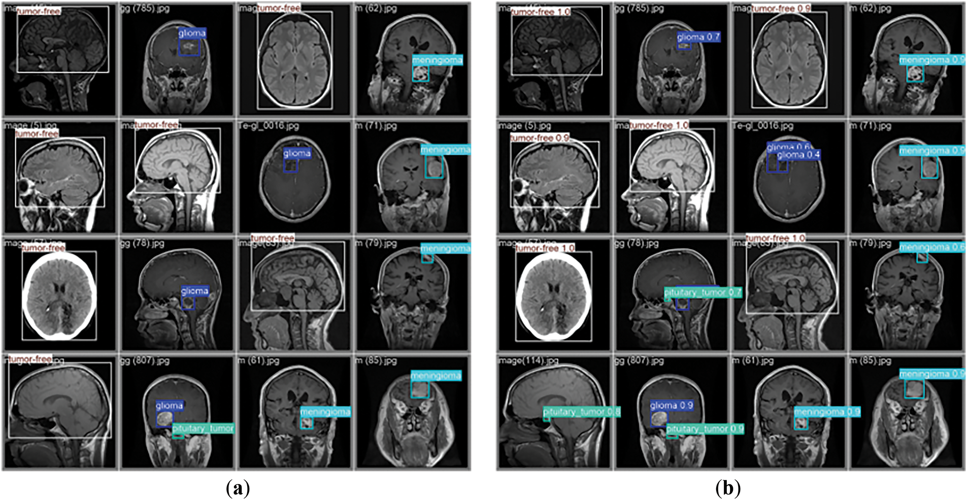
Figure 12: Model detection results. (a) The diagram of the GT annotation. (b) The results of the CMS-YOLO prediction

4.2.2 Comparative Analysis of Different Algorithms

This study conducts multiple sets of comparison tests on the dataset used to train the CMS-YOLO model, verifying the efficacy of the suggested model on the same dataset. The outcomes are displayed in Table 5. The CMS-YOLO model achieves a precision of 94.80%, which is the second highest among all algorithms, with a 1% improvement over the original model. Furthermore, the CMS-YOLO model outperforms all other algorithms in the recall, F1−score, and mAP50, achieving values of 93.60%, 94.20%, and 96.20%, respectively, which are the highest among all algorithms. The mAP50-95 of the CMS-YOLO model is improved by 1% compared to the original model, indicating that the CMS-YOLO model performs better overall. In contrast, YOLOv5 and YOLOv8 performed well, but their recall, mAP50 and mAP50-95 was lower than that of the CMS-YOLO model. This may be because the change in the model structure enables better feature extraction and feature fusion, thereby helping to capture the subtle features in the MRI images more precisely. In addition, the data processing method enhances the dataset’s quality and avoids problems such as gradient explosion during model training.

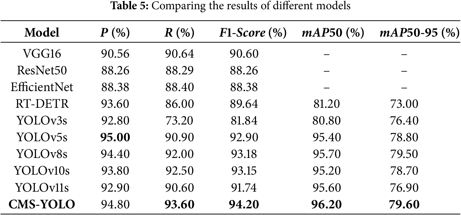
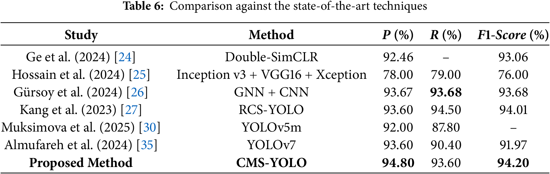
The performance results of several research techniques detecting brain tumors are shown in Table 6. The CMS-YOLO model proposed in this study attains the highest precision and F1−score, and achieves the second-highest recall, demonstrating the superiority of the CMS-YOLO model. This achievement can primarily be attributed to:

(1)   The optimized C2f module can capture more global context information. Moreover, with the addition of the MSAA module, it can achieve different scale feature fusion, which makes it possible to acquire more detailed feature information.

(2)   Modifying the loss function can improve the accuracy of bounding box regression, enhance the model’s adaptability to small targets and complex backgrounds, and increase the model’s robustness to shape changes.

4.3 Ablation Experiment

In order to verify the effectiveness and role of the introduced components, and the effect of different configurations on the performance of the CMS-YOLO, a series of ablation experiments were conducted on the brain tumor dataset. The results of the experiments are shown in Table 7. The evaluation metrics used include F1−score, mAP50, and mAP50-95.

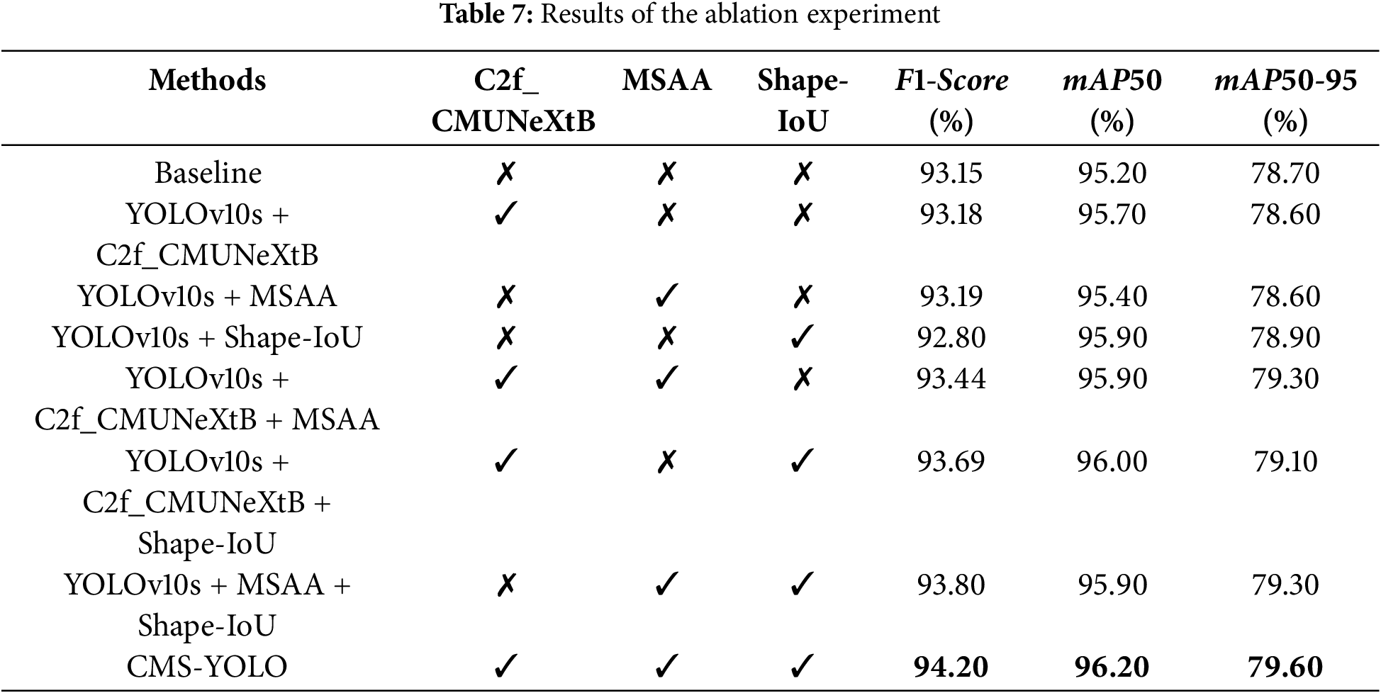
“✓” indicates that the component was introduced into the model, and a “✗” indicates that the component is excluded from the model. When C2f_CMUNeXtB, MSAA, and Shape-IoU are respectively introduced into the baseline network, the model’s precision either slightly decreases or increases, but the improvement of mAP50 is significant, suggesting that these modules or methods play a positive role in improving the model’s detection accuracy. When the C2f_CMUNeXtB and MSAA modules are introduced simultaneously, the model’s performance is significantly improved, with F1−score, mAP50, and mAP50-95 of 93.44%, 95.9% and 79.4%, respectively. This demonstrated that these two modules working together can capture the features more fully and have a synergistic effect on the model’s performance. In addition, performance is further improved by introducing MSAA and Shape-IoU simultaneously. Ultimately, the integration of these three components into the model achieves the highest performance, highlighting the significant contributions of C2f_CMUNeXtB, MSAA, and Shape-IoU. Each of these elements positively influences the model’s detection capabilities and their combined interaction results in optimal performance.

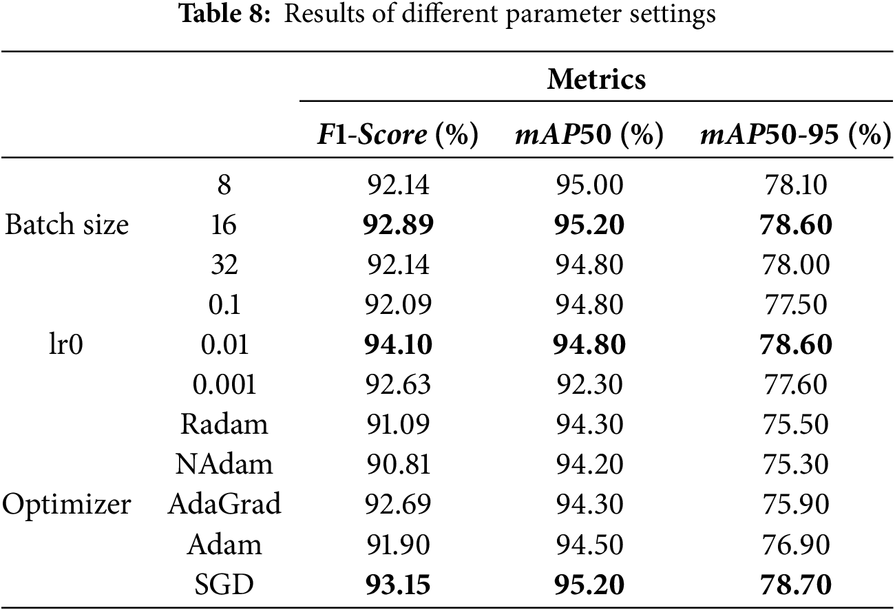
Table 8 presents the results of the evaluation metrics of the model with various parameter settings. As can be seen from the table, the F1−score, mAP50, and mAP50-95 of the model are enhanced as the Batch size increases, and the model presents optimal performance when the Batch size is 16. However, in general, the change of each metric is small when the Batch size changes. This may be attributed to the fact that the Batch size mainly affects whether the gradients can stably and accurately reflect the direction and magnitude of the model parameter updates during training. However, under the data distribution and model architecture employed in this experiment, this stability has a limited impact on the model performance, indicating that the effect of Batch size on the model is weak. When the value of lr0 is 0.01, the performance of each metric is excellent. The fluctuation of the metrics is significant under different values of lr0, which may be because the learning rate directly affects the convergence state of the model. When the lr0 is set too large, it causes the model to skip the optimal solution and be prone to overfitting. Conversely, when it is too small, it leads to slower convergence of the model. This indicates that the model is more sensitive to the lr0. With different optimizers, there are noticeable differences in each metric. The model achieves the best performance across all metrics when using the SGD optimizer, indicating that the SGD optimizer can update model parameters more effectively and find the optimal solution in this study. This demonstrates the model’s high sensitivity of optimizer selection. These results highlight the critical roles of Batch size, lr0, and optimizer in optimizing metrics such as F1−score, mAP50, and mAP50-95, and improving the model’s overall performance. Therefore, in practical applications, appropriate parameters should be selected according to the specific data distribution and task requirements.

4.4 Grad-CAM Visualization

Visualization methods provide insight into the internal workings of a model, facilitating an understanding of how the model makes predictions and enhancing model transparency and trust. Gradient-weighted Class Activation Mapping [36] (Grad-CAM) is a common method for explaining model decisions. It operates by assigning weights to the feature maps of a convolutional layer based on the gradient of the target class with respect to the final output. This enables Grad-CAM to generate a class activation map that highlights the regions of the input image upon which the model focuses when making class-specific predictions, thereby offering insight into the model’s decision-making process.

Fig. 13 shows the original images and the Grad-CAM visualization results of glioma, meningioma, pituitary tumor, and no tumor. The model frames out the lesion area and highlights it in red when it identifies a tumor. The algorithm identifies the entire brain region as healthy when no lesion is seen in a tumor-free picture. This visualization method provides an intuitive representation of how the model focuses on image regions and identifies different brain tumors. This enhances physicians’ understanding of how the model makes decisions. It serves as a valuable diagnostic aid, supporting more accurate clinical assessments.

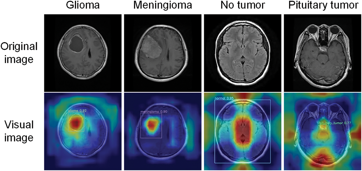
Figure 13: Visualization results

5  Conclusion

In this study, we propose the CMS-YOLO algorithm, which is specifically designed to identify brain tumors in MRI images. This method is capable of accurately localizing brain tumors and reducing the occurrence of false positives and false negatives, which are caused by the complex background and the diversity of brain tumors in morphology and size. Redesigning the C2f module to more effectively capture global context information, which helps to extract deeper lesion region features. By incorporating the MSAA module to aid in the fusion of multi-scale features in terms of both channel and spatial dimensions, the algorithm enhances the model’s capability to handle complex backgrounds and improves the extraction of features from small targets, thereby increasing the model’s detection accuracy. The Shape-IoU loss function takes into account the impact of the bounding box’s shape and scale on its regression when it is introduced, addressing the missed detection rate caused by differences in the morphology and size of brain tumors. This enhancement significantly improves the model’s precision and robustness in detecting and localizing brain tumors. Experimental results demonstrate that the algorithm’s precision and recall reach 94.80% and 93.60%, respectively, and it attains a mAP50 of 96.20% and a mAP50-95 of 79.60%, These values surpass those of other state-of-the-art methods, and the enhancement of these metrics highlights the effectiveness and generalization ability of the proposed method for detecting brain tumors in MRI images.

In clinical decision-making, the interpretability of the model is particularly important. This study utilizes the Grad-CAM visualization method to explain the model’s decision-making process, facilitate the researchers’ understanding of the model’s internal operation mechanism, and provide doctors with a basis for informed decision-making. These results show that the proposed model not only achieves faster and more accurate detection of brain tumors but also assists doctors in early diagnosis in practical scenarios, thereby reducing diagnostic time. This can help to speed up the treatment process and gain valuable treatment time for patients in critical condition. Although CMS-YOLO shows better results in achieving fast and accurate detection of brain tumors, there are still some limitations in this study. Regarding the dataset, various categories have been considered comprehensively. However, the number of brain tumor categories it covers is still few, making it challenging to cover the diversity of brain tumor features comprehensively. This limits the model’s ability to learn and recognize various types of complex brain tumor features to a certain extent. As the YOLOv10 algorithm requires high computational resources in its structural design, it inevitably brings about a more significant consumption of computational resources when making further improvements to the model. Meanwhile, in terms of research resources, the performance of the hardware devices is limited and unable to support large-scale data-parallel computing.

In future studies, (1) further exploration of the model’s detection performance on more categories of brain tumors is planned, especially brain tumors with complex features and blurred edges; (2) exploring advanced lightweight fusion models. This has an opportunity to decrease the number of network parameters and enhance the capability to capture complex features. Additionally, introducing a broader range of diverse datasets to improve the model’s generalization capacity and performance; (3) Conduct further clinical validation of the model to test its reliability and generalizability in different clinical settings, thereby providing reliable support for clinical diagnosis and treatment.

Acknowledgement: The authors would like to express their gratitude for the valuable feedback and suggestions provided by all the anonymous reviewers and the editorial team.

Funding Statement: This work was supported in part by the National Natural Science Foundation of China under Grants 61861007; in part by the Guizhou Province Science and Technology Planning Project ZK [2021]303; in part by the Guizhou Province Science Technology Support Plan under Grants [2022]264, [2023]096, [2023]412 and [2023]409.

Author Contributions: The authors confirm their contribution to the paper as follows: Study conception and design: Li Li, Xiao Wang, Qinmu Wu; data collection: Li Li, Xiao Wang, Qinmu Wu, Zhiqin He; analysis and interpretation of results: Li Li, Ran Ding, Linlin Luo, Zhiqin He; draft manuscript preparation: Li Li, Xiao Wang. All authors reviewed the results and approved the final version of the manuscript.

Availability of Data and Materials: To validate the model, we used the following public dataset: https://www.kaggle.com/datasets/ahmedsorour1/mri-for-brain-tumor-with-bounding-boxes (accessed on 10 June 2025).

Ethics Approval: Not applicable.

Conflicts of Interest: The authors declare no conflicts of interest to report regarding the present study.

References

1. Berghout T. The neural frontier of future medical imaging: a review of deep learning for brain tumor detection. J Imaging. 2025;11(1):2. doi:10.3390/jimaging11010002. [Google Scholar] [PubMed] [CrossRef]

2. Bray F, Laversanne M, Sung H, Ferlay J, Siegel R, Soerjomataram I, et al. Global cancer statistics 2022: GLOBOCAN estimates of incidence and mortality worldwide for 36 cancers in 185 countries. A Cancer J Clin. 2024;74(03):229–63. doi:10.3322/caac.21834. [Google Scholar] [PubMed] [CrossRef]

3. Han B, Zheng R, Zeng H, Wang S, Sun K, Chen R, et al. Cancer incidence and mortality in China, 2022. J Natl Cancer Cent. 2024;4(01):47–53. doi:10.1016/j.jncc.2024.01.006. [Google Scholar] [PubMed] [CrossRef]

4. Wang F. Research on brain tumor lesion detection algorithm based on deep learning [dissertation]. Wuhan, China: Wuhan Institute of Technology; 2023. (In Chinese). doi:10.27727/d.cnki.gwhxc.2023.000089. [Google Scholar] [CrossRef]

5. Batool A, Byun Y. Brain tumor detection with integrating traditional and computational intelligence approaches across diverse imaging modalities—challenges and future directions. Comput Biol Med. 2024;175(1):108412. doi:10.1016/j.compbiomed.2024.108412. [Google Scholar] [PubMed] [CrossRef]

6. Ge M. Zhejiang Provincial People’s Hospital: seize the new track of artificial intelligence and cultivate new quality productive forces in the medical field. China Health. 2025;04:103–5. (In Chinese). doi:10.15973/j.cnki.cn11-3708/d.2025.04.040. [Google Scholar] [CrossRef]

7. Deng H. Heavyweight! Tsinghua University Establishes Artificial Intelligence Hospital [Internet]. Beijing, China: Tsinghua University; 2025 [cited 2025 Apr 27]. Available from: https://www.tsinghua.edu.cn/info/1182/118501.htm. [Google Scholar]

8. Zhou X, Liu H, Wang T, Liu X, Liu F, Kang D. Challenges and future directions of medicine with artificial intelligence. Chin J Clin Thorac Cardiovasc Surg. 2025;32(02):244–51. (In Chinese). [Google Scholar]

9. Chai J, Li A, Zhang H, Ma Y, Mei X, Ji Ma. 3D multi-organ segmentation network combining local and global features and multi-scale interaction. J Image Graph. 2024;29(03):655–69. (In Chinese). [Google Scholar]

10. Zhao J, Liu L, Yang X, Cui Y, Li D, Zhang H, et al. A medical image segmentation method for rectal tumors based on multi-scale feature retention and multiple attention mechanisms. Med Phys. 2024;51(05):3275–91. doi:10.1002/mp.17044. [Google Scholar] [PubMed] [CrossRef]

11. Song Z, Luo C, Li T, Chen H. Classification of thoracic diseases based on attention mechanisms and two-branch networks. Comput Sci. 2024;51(S2):219–24. (In Chinese). [Google Scholar]

12. Subash J, Kalaivani S. Dual-stage classification for lung cancer detection and staging using hybrid deep learning techniques. Neural Comput Appl. 2024;36(14):8141–61. doi:10.1007/s00521-024-09425-3. [Google Scholar] [CrossRef]

13. Wang Y, Yang K, Wen Y, Wang P, Hu Y, Lai Y, et al. Screening and diagnosis of cardiovascular disease using artificial intelligence-enabled cardiac magnetic resonance imaging. Nat Med. 2024;30(5):1471–80. doi:10.1038/s41591-024-02971-2. [Google Scholar] [PubMed] [CrossRef]

14. Qureshi K, Alhudhaif A, Ali M, Qureshi M, Jeon G. Self-assessment and deep learning-based coronavirus detection and medical diagnosis systems for healthcare. Multimed Syst. 2022;28(4):1439–48. doi:10.1007/s00530-021-00839-w. [Google Scholar] [PubMed] [CrossRef]

15. Cai Y, Luo M, Yang W, Xu C, Wang P, Xue G, et al. The deep learning framework iCanTCR enables early cancer detection using the T-cell receptor repertoire in peripheral blood. Cancer Res. 2024;84(11):1915–28. doi:10.1158/0008-5472.CAN-23-0860. [Google Scholar] [PubMed] [CrossRef]

16. Diao X, Wang X, Qin J, Wu Q, He Z, Fan X. A Review of the application of artificial intelligence in orthopedic diseases. Comput Mater Contin. 2024;78(02):2617–65. doi:10.32604/cmc.2024.047377. [Google Scholar] [CrossRef]

17. Mohamed M, Mahesh T, Vinoth K, Guluwadi S. Enhancing brain tumor detection in MRI images through explainable AI using Grad-CAM with Resnet 50. BMC Med Imaging. 2024;24(1):107. doi:10.1186/s12880-024-01292-7. [Google Scholar] [PubMed] [CrossRef]

18. Tian H, Wang Y, Xiao H. Full-automatic brain tumor segmentation based on multimodal feature recombination and scale cross attention mechanism. Chin J Lasers. 2024;51(21):129–38. (In Chinese). [Google Scholar]

19. Ghazouani F, Vera P, Ruan S. Efficient brain tumor segmentation using Swin transformer and enhanced local self-attention. Int J Comput Assist Radiol Surg. 2024;19(2):273–81. doi:10.1007/s11548-023-03024-8. [Google Scholar] [PubMed] [CrossRef]

20. Li P, Li Z, Wang Z, Li C, Wang M. mResU-Net: multi-scale residual U-Net-based brain tumor segmentation from multimodal MRI. Med Biol Comput. 2024;62(3):641–51. doi:10.1007/s11517-023-02965-1. [Google Scholar] [PubMed] [CrossRef]

21. Wu B, Shi DH, Lü D. Brain tumor classification based on federated learning with improved CBAM-ResNet18. Comput Syst Appl. 2024;33(04):39–49. (In Chinese). doi:10.15888/j.cnki.csa.009469. [Google Scholar] [CrossRef]

22. Sankar M, Baiju BV, Preethi D, Ananda K, Sandeep KM, Mohd AS. Efficient brain tumor grade classification using ensemble deep learning models. BMC Med Imaging. 2024;24(1):297. doi:10.1186/s12880-024-01476-1. [Google Scholar] [PubMed] [CrossRef]

23. Nassar SE, Yasser I, Amer HM, Mohamed MA. A robust MRI-based brain tumor classification via a hybrid deep learning technique. J Supercomput. 2024;80(2):2403–27. doi:10.1007/s11227-023-05549-w. [Google Scholar] [CrossRef]

24. Ge Y, Xu L, Wang X, Que Y, Piran M. A novel framework for multimodal brain tumor detection with scarce labels. IEEE J Biomed Health Inform. 2024;2024:1–14. doi:10.1109/JBHI.2024.3467343. [Google Scholar] [PubMed] [CrossRef]

25. Hossain S, Chakrabarty A, Gadekallu T, Alazab M, Jalil Piran M. Vision transformers, ensemble model, and transfer learning leveraging explainable AI for brain tumor detection and classification. IEEE J Biomed Health Inform. 2024;28(3):1261–72. doi:10.1109/JBHI.2023.3266614. [Google Scholar] [PubMed] [CrossRef]

26. Gürsoy E, Kaya Y. Brain-GCN-Net: graph-convolutional neural network for brain tumor identification. Comput Biol Med. 2024;180(1):108971. doi:10.1016/j.compbiomed.2024.108971. [Google Scholar] [PubMed] [CrossRef]

27. Kang M, Ting C, Ting F, Phan R. RCS-YOLO: a fast and high-accuracy object detector for brain tumor detection. In: Proceedings of the Medical Image Computing and Computer Assisted Intervention (MICCAI); 2023 Oct 8–12; Vancouver, BC, Canada. doi:10.1007/978-3-031-43901-8_57. [Google Scholar] [CrossRef]

28. Chen A, Lin D, Gao Q. Enhancing brain tumor detection in MRI images using YOLO-NeuroBoost model. Front Neurol. 2024;15:1445882. doi:10.3389/fneur.2024.1445882. [Google Scholar] [PubMed] [CrossRef]

29. Costa Nascimento J, Gomes Marques A, Nascimento Souza L, Mattos Dourado C, Silva Barros A, Albuquerque V, et al. A novel generative model for brain tumor detection using magnetic resonance imaging. Comput Med Imaging Graph. 2025;121(10):102498. doi:10.1016/j.compmedimag.2025.102498. [Google Scholar] [PubMed] [CrossRef]

30. Muksimova S, Umirzakova S, Mardieva S, Iskhakova N, Sultanov M, Cho Y. A lightweight attention-driven YOLOv5m model for improved brain tumor detection. Comput Biol Med. 2025;188(3):109893. doi:10.1016/j.compbiomed.2025.109893. [Google Scholar] [PubMed] [CrossRef]

31. Wang A, Chen H, Liu L, Chen K, Lin Z, Han J, et al. YOLOv10: real-time end-to-end object detection. arXiv: 2405.14458. 2024. [Google Scholar]

32. Tang F, Ding J, Wang L, Ning C, Zhou K. CMUNeXt: an efficient medical image segmentation network based on large kernel and skip fusion. arXiv:2308.01239. 2023. [Google Scholar]

33. Liu M, Dan J, Lu Z, Yu Y, Li Y, Li X. CM-UNet: hybrid CNN-Mamba UNet for remote sensing image semantic segmentation. arXiv:2405.10530. 2024. [Google Scholar]

34. Zhang H, Zhang S. Shape-IoU: more accurate metric considering bounding box shape and scale. arXiv:2312.17663. 2023. [Google Scholar]

35. Almufareh MF, Imran M, Khan A, Humayun M, Asim M. Automated brain tumor segmentation and classification in MRI using YOLO-based deep learning. IEEE Access. 2024;12(2):16189–207. doi:10.1109/ACCESS.2024.3359418. [Google Scholar] [CrossRef]

36. Selvaraju R, Cogswell M, Das A, Vedantam R, Parikh D, Batra D. Grad-CAM: visual explanations from deep networks via gradient-based localization. In: Proceedings of the IEEE International Conference on Computer Vision (ICCV); 2017 Oct 22–29; Venice, Italy. doi:10.1109/ICCV.2017.74. [Google Scholar] [CrossRef]