
 Submit a Paper
 Propose a Special lssue
 Open Access
ARTICLE

A YOLOv11 Empowered Road Defect Detection Model
1 Anhui Conch Global Intelligent Technology Co., Ltd., Wuhu, 241204, China
2 School of Computer Science and Information Engineering, Shanghai Institute of Technology, Shanghai, 201418, China
* Corresponding Author: Peng Luo. Email:
Computers, Materials & Continua 2025, 85(1), 1073-1094. https://doi.org/10.32604/cmc.2025.066078
Received 28 March 2025; Accepted 24 June 2025; Issue published 29 August 2025
 View Full Text
 Download PDF
Abstract
Roads inevitably have defects during use, which not only seriously affect their service life but also pose a hidden danger to traffic safety. Existing algorithms for detecting road defects are unsatisfactory in terms of accuracy and generalization, so this paper proposes an algorithm based on YOLOv11. The method embeds wavelet transform convolution (WTConv) into the backbone’s C3k2 module to enhance low-frequency feature extraction while avoiding parameter bloat. Secondly, a novel multi-scale fusion diffusion network (MFDN) architecture is designed for the neck to strengthen cross-scale feature interactions, boosting detection precision. In terms of model optimization, the traditional downsampling method is discarded, and the innovative Adown (adaptive downsampling) technique is adopted, which streamlines the parameter scales while effectively mitigating the information loss problem during downsampling. Finally, in this paper, we propose Wise-PIDIoU by combining WiseIoU and MPDIoU to minimize the negative impact of low-quality anchor frames and enhance the detection capability of the model. The experimental results indicate that the proposed algorithm achieves an average detection accuracy of 86.5% for mAP@50 on the RDD2022 dataset, which is 2% higher than the original algorithm while ensuring that the amount of computation is basically unchanged. The number of parameters is reduced by 17%, and the F1 score is improved by 3%, showing better detection performance than other algorithms when facing different types of defects. The excellent performance on embedded devices proves that the algorithm also has favorable application prospects in practical inspection.Keywords
Roads are a crucial component of a country’s infrastructure, closely linked to economic development and everyday life. However, over time, road structures can deteriorate due to factors such as climate change and insufficient maintenance. This deterioration can result in various road defects, including cracks, fissures, and potholes. Such defects can create a chain reaction that complicates vehicle operation and may even lead to life-threatening traffic disasters, posing risks to public safety and property [1]. In light of these issues, it has become essential to develop efficient and accurate mechanisms for detecting road defects.
Early road defect detection relied on manual inspection, which was dependent on personal experience. This approach often led to inconsistent results and required substantial human resources. Consequently, the detection process was inefficient, the results were subjective, and ensuring accuracy became challenging. With advancements in image processing technology, various methods such as threshold segmentation, edge detection, and wavelet transformation have emerged for road defect detection. However, images of road defects often feature complex backgrounds with low contrast between the defects and their surroundings. To effectively extract meaningful features from these images, more sophisticated image processing techniques are typically necessary. Additionally, road defect images are susceptible to a range of factors, including variations in lighting, shadows, angles, and weather conditions, which can negatively impact the performance of image processing-based detection methods, resulting in diminished robustness during practical applications.
Road defects are very diverse, typically including cracks, potholes, and other types of damage [2], and the dataset may contain many confounding factors. For example, the complexity and variability of road conditions, along with factors such as light, water pollution, and oil pollution, will affect the algorithm’s recognition performance. Therefore, this paper adopts the RDD-2022 dataset, which has relatively complete road defects categories, and the categories mainly include longitudinal cracks, transverse cracks, mesh cracks, and road repair. The YOLO series algorithm has recently been upgraded, with YOLOv11 achieving notable advancements in both accuracy and detection speed. It is essential to integrate road defect detection with this latest algorithm. To address these challenges, this paper proposes a new model that enhances YOLOv11 for detecting road defects by employing techniques such as multi-scale feature combination and a diffusion network. The specific contributions of this paper include:
(1) WTConv (Wavelet Transform Convolution) [3] is added to some of the C3k2 modules in the backbone network, which helps the model see a larger area and effectively gather important low-frequency information using fewer parameters.
(2) MFDN (Multi-scale fusion and diffusion networks) is introduced in the neck structure to combine feature information from various levels, allowing the model to focus more on local details.
(3) Adown (Adaptive Downsample) [4] is used in the downsampling module to obtain richer feature information while reducing redundant information.
(4) In terms of the loss function, the advantages of WiseIoU [5] and MPDIoU [6] are combined to solve the problem that traditional IoU is not sensitive enough to center shifts. We reduce the negative impact of low-quality anchor frames to enhance the model’s detection capabilities.
This paper organizes its structure as follows: Section 2 will give an overview of the primary algorithms for detecting road defects, Section 3 introduces the overall structure of the model and the improved design, Section 4 presents information about the experiments, Section 5 conducts the comparative experiments and result analysis, Section 6 introduces the limitations of this paper and the subsequent solutions, and Section 7 concludes the paper.
In recent times, the advancement of deep learning technology has been nothing short of astonishing. Algorithms that utilize deep learning for object detection are adept at identifying complex patterns within images and efficiently isolating features, even in challenging backgrounds. As a result, deep learning has emerged as a dominant force in the field of object detection, greatly enhancing the progress of systems for detecting road defects. These algorithms can be categorized into two types: two-stage and single-stage, based on how they generate candidate target regions.
Popular two-stage detection algorithms such as Fast R-CNN [7], Faster R-CNN [8], Mask R-CNN [9], Cascade R-CNN [10], and SPPNet [11] have been widely studied in the field. Building on this foundation, Li et al. [12] integrated SENet with Faster R-CNN to bolster the model’s attention mechanism, thoroughly investigating SENet’s influence across various levels and showcasing its effectiveness in pavement crack detection. Meanwhile, Tang et al. [13] tackled the challenge of limited sample sizes by incorporating a transfer learning approach rooted in multi-source adaptive balanced TrAdaBoost during network training, which significantly boosted crack detection accuracy. In another study, Chen et al. [14] leveraged DenseNet as the backbone for Mask R-CNN and employed a feature pyramid network to fuse multi-scale features, yielding superior detection outcomes. Additionally, a novel approach presented in [15] introduced a Cascade R-CNN framework that combines the MS-Feature Pyramid Network with a dual-channel attention fusion algorithm, enabling robust adaptability to road defects across diverse backgrounds. Due to the slow processing speed of the two-stage algorithm, the model structure is relatively complex, and it usually requires more computing resources and memory, which is often difficult to implement on embedded systems. With the development of technology, one-stage object detection algorithms have developed rapidly. This is because the generation of candidate boxes and the classification regression operation are combined into one, and a separate Region Proposal Network (RPN) is not required. Therefore, single-stage algorithms have a more concise structure and faster detection speed while also reducing the cost of model deployment. Although the detection accuracy of single-stage algorithms may lag behind that of two-stage algorithms, the gap is gradually closing as the technology develops.
Among single-stage detection algorithms, RetinaNet, SSD, and YOLO are widely recognized. Li et al. [16] introduced a novel detection module by leveraging MobileNet and SSD, incorporating receptive field enhancement and deep separable convolution fusion to enrich feature information. This approach significantly boosted algorithm accuracy while maintaining real-time detection capabilities. Meanwhile, Liu et al. [17] tackled data scarcity by designing an unsupervised generative adversarial network with a self-attention mechanism. They combined MobileNetV2 with the CBAM attention mechanism and refined YOLOv4 using Focal loss for confidence optimization. The resulting algorithm demonstrated faster inference speeds, reduced memory consumption, and proved effective in practical applications. Roy et al. [18] enhanced YOLOv5 by integrating DenseNet into its backbone network. They employed the CBAM attention module and an additional feature fusion layer for deep feature extraction, complemented by Swin-Transformer for detection head optimization. These modifications led to superior overall performance compared to contemporary models. Similarly, Fang et al. [19] augmented ShuffleNetV2 with the ECA attention module, creating Shuffle-ECANet, which was then integrated into YOLOv5s. They utilized BiFPN in the neck network to enhance feature representation and adopted Focal-EIOU for localization loss, resulting in higher-quality anchor boxes. This streamlined model size, improved detection speed, and made it more suitable for embedded systems. Chen et al. [20] focused on intelligent road surface defect detection by employing the K-means algorithm with 1-IoU as the sample distance to recluster anchors, optimizing anchor box parameters. They also integrated the CBAM attention mechanism to strengthen feature extraction. These enhancements led to notable improvements in both accuracy and detection speed over the baseline model. In another study [21], SPD-Conv was introduced into YOLOv8’s backbone network to replace traditional convolution, while the ASF-YOLO neck network architecture was adopted. To minimize redundant computations, the FasterNet module was incorporated into C2f, and Wise-IoU was used to optimize the loss function. Experimental results confirmed the algorithm’s effectiveness in real-time detection tasks.
The YOLOv11 algorithm, the most recent addition to the YOLO series, was released by Ultralytics on 30 September 2024. Its structural design is depicted in Fig. 1 YOLOv11 structure diagram. A comparison of YOLOv11 with previous algorithms reveals the following innovations.
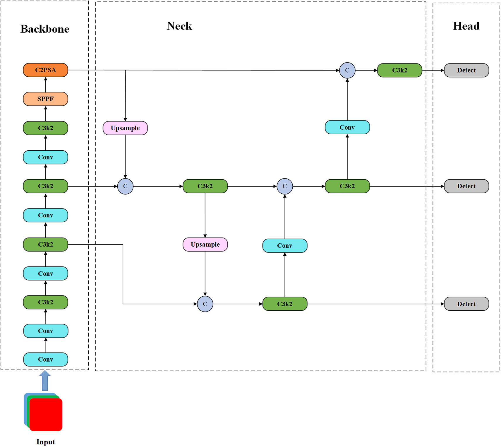
Figure 1: YOLOv11 structure diagram
Replace the C2f module with the C3k2 module, as shown in Fig. 2. (a) represents the structure of C2f in YOLOv8, (b) represents the structure of C3k2 in YOLOv11, (c) represents the structure of C3k in C3k2, and (d) represents the structure of Bottleneck. Bottleneck serves as the basic module of C2f in YOLOv8 and C3k2 in YOLOv11. An option exists for utilizing a shortcut to propagate richer gradient information, which aids in constructing complex CSP structures (Cross Stage Partial). In C3k2, there is flexibility regarding the use of C3k. When set to False, the standard structure of C3k2 resembles that of C2f, employing a fixed Bottleneck layer. When true, the C3k structure gets utilized, allowing for the setting of different sizes of convolutional kernels during C3k initialization. This adaptability better accommodates the features of images of varying sizes. Therefore, C3k2 offers more flexible feature extraction options compared to C2f.
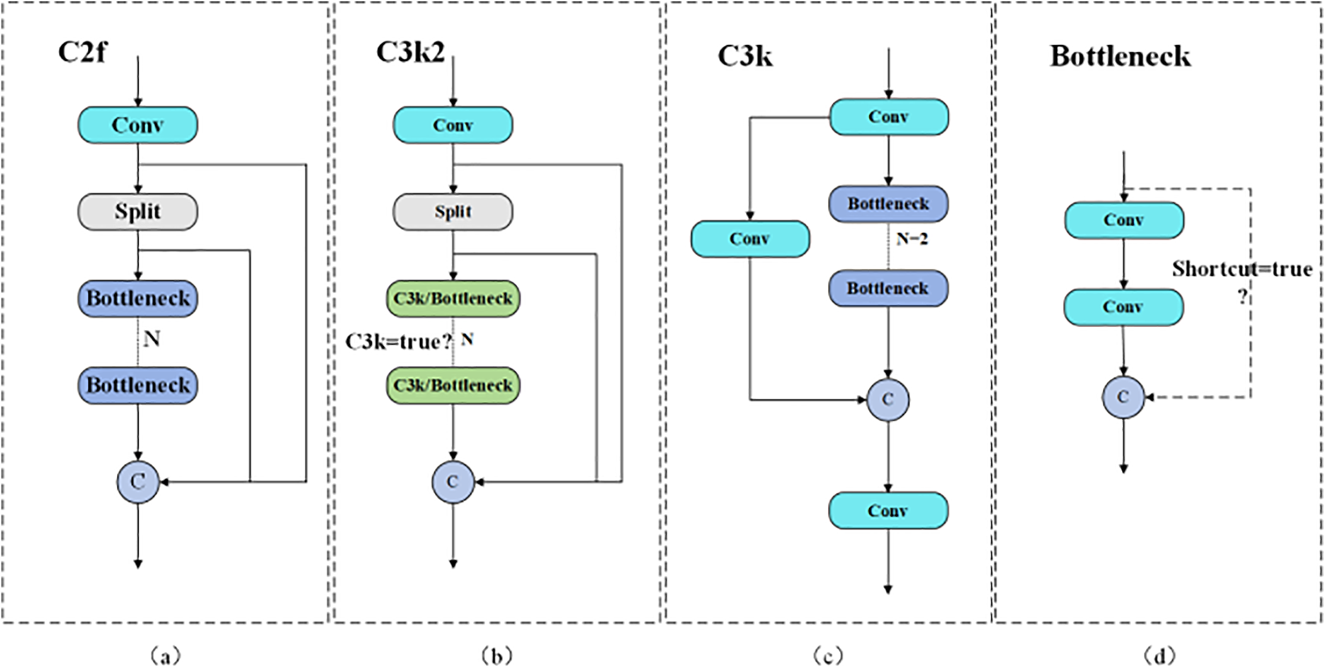
Figure 2: Comparison of C2f and C3k2 modules
Another important innovation of YOLOv11 is the addition of the C2PSA module after the SPPF module, as shown in Fig. 3. C2PSA combines the CSP structure and PSA (Pyramid Squeeze Attention) to obtain richer information about the echelon flow while making the model pay more attention to spatial information. The innovation of YOLOv11 in the detection head is the use of depth-separable convolutions, as shown in Fig. 4. In the classification branch of the head, YOLOv11 replaces the original 3 × 3 ordinary convolution with a combination of DWConv (Depthwise Convolution) and 1 × 1 ordinary convolution, which greatly reduces the number of parameters and the amount of calculation in the detection head while ensuring the performance of the network.
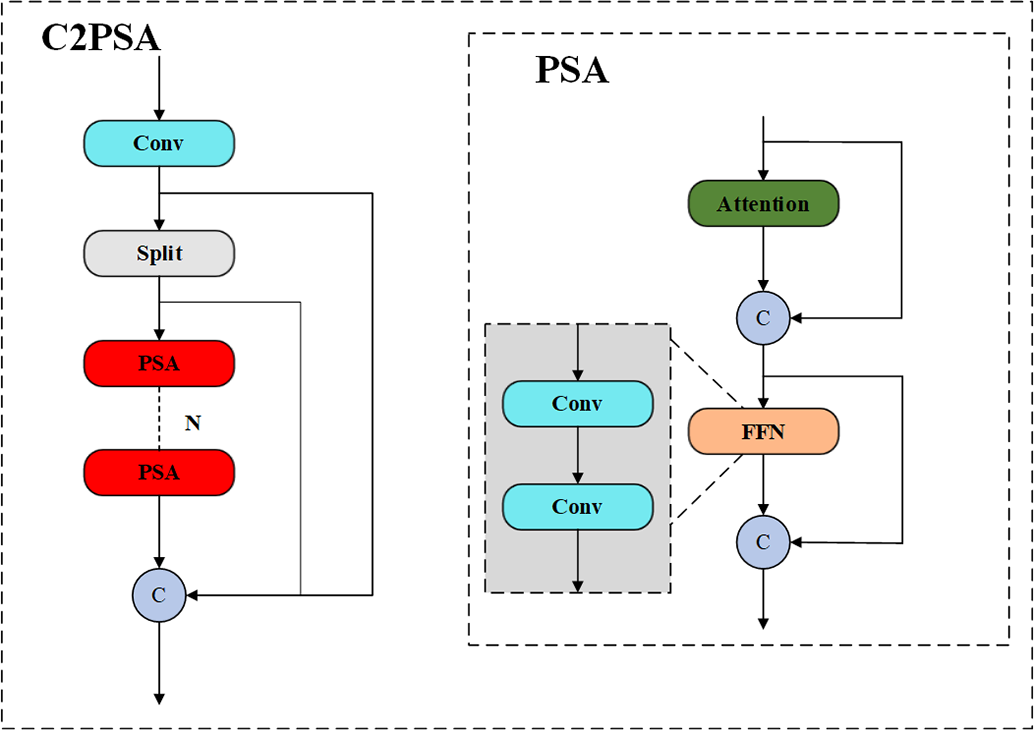
Figure 3: Structural diagram of C2PSA
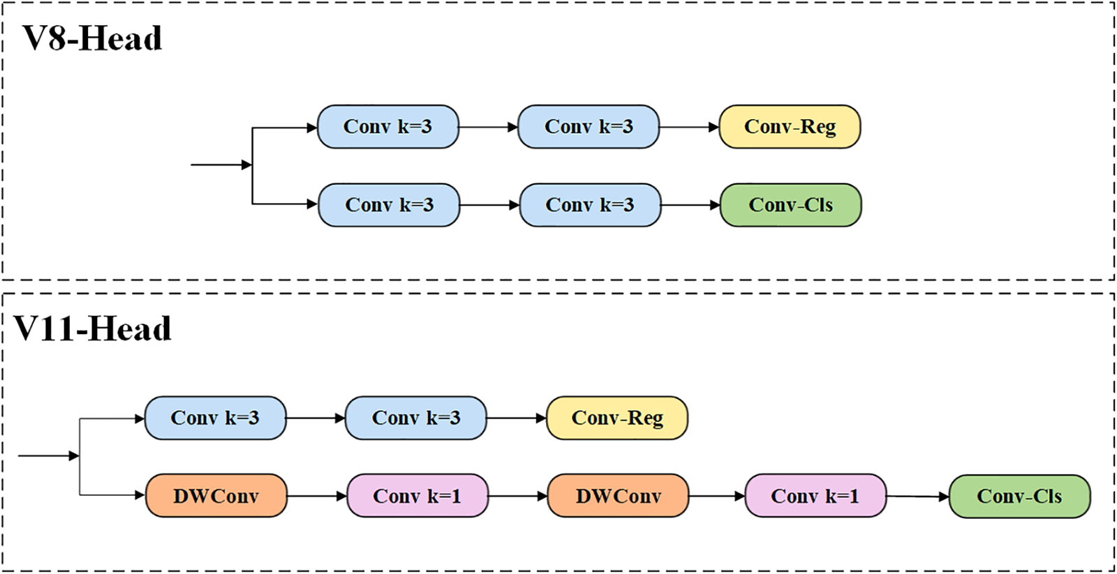
Figure 4: Comparison of the head structures of YOLOv11 and YOLOv8
In comparison to earlier algorithms, YOLOv11 enhances detection accuracy and simultaneously minimizes model parameters, leading to improved computational efficiency. This makes it particularly well-suited for deployment on devices with limited resources.
This paper’s algorithm is an improved version of YOLOv11, which aims to enhance the model’s feature extraction ability, make the model more robust, and perform better on resource-constrained devices. The structure is shown in Fig. 5. Fig. 6 presents the overall flowchart of this paper.
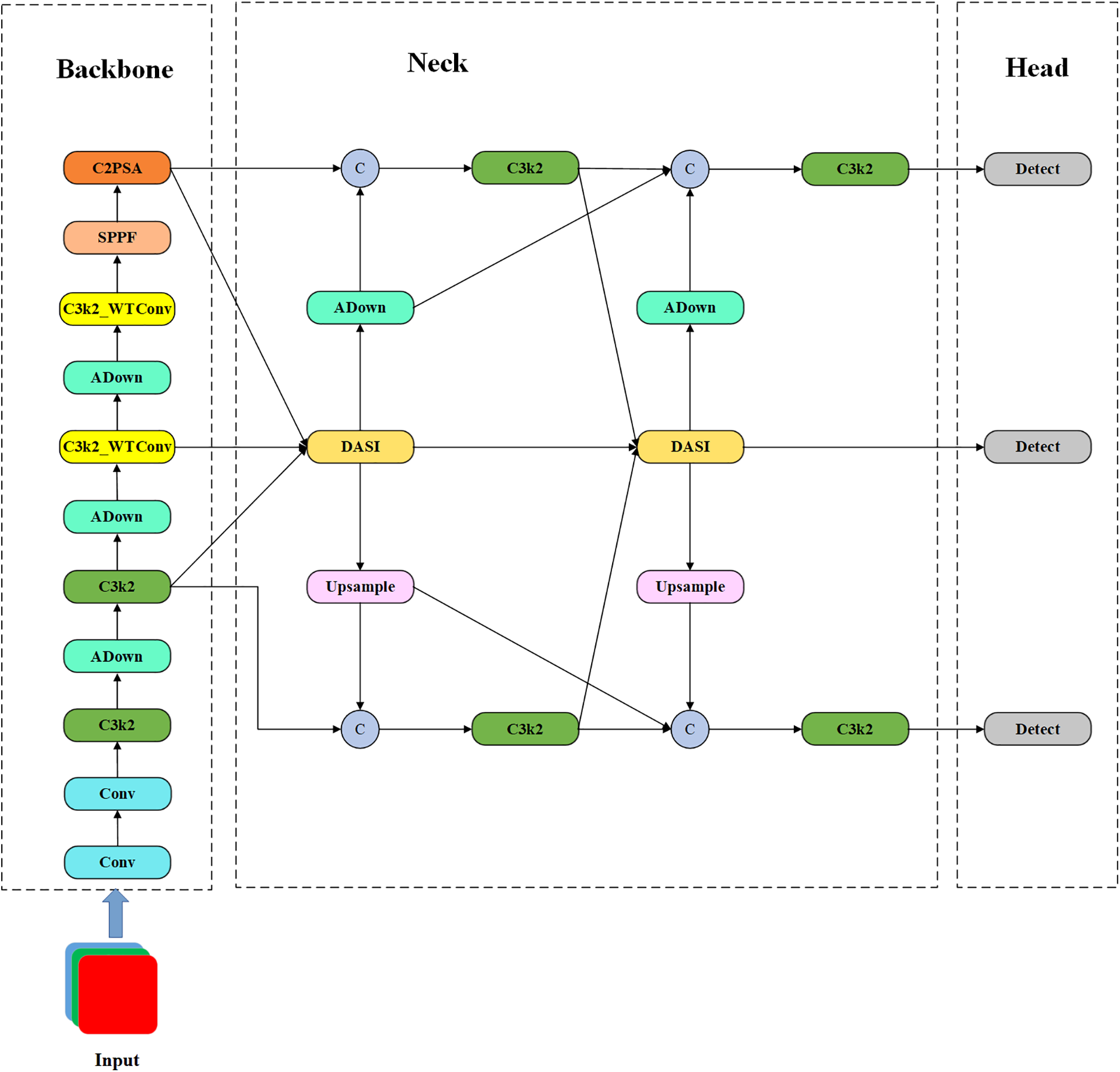
Figure 5: Structure of the empowered YOLO model
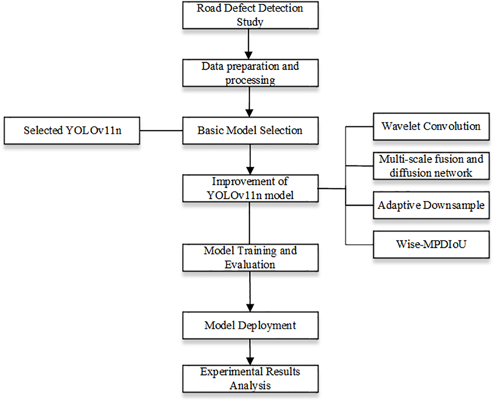
Figure 6: Flowchart of this paper
3.3 Wavelet Transform Convolution
The C3k2 module in YOLOv11 has been demonstrated to enhance the model’s capacity to extract richer gradient information; however, the receptive field size is constrained. Therefore, this paper adds WTConv to C3k2, as shown in Fig. 7, which mainly replaces the second ordinary convolution with WTConv in the Bottleneck part. Achieving a larger receptive field with fewer parameters enables the model to concentrate more on low-frequency information, thus enhancing its road defect detection ability.
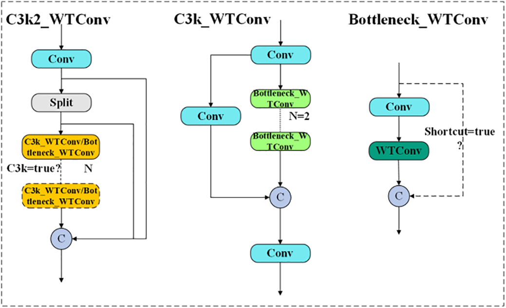
Figure 7: C3K2_WTConv structure diagram
Due to the simplicity and efficiency of the Haar wavelet, WTConv selects it as the wavelet basis. The one-dimensional Haar wavelet basis is mainly represented by a low-pass filter and a high-pass filter. The two-dimensional Haar WT is built on the basis of the one-dimensional Haar wavelet, and the four filters used are shown in Eq. (1).
For the input image
As depicted in Fig. 8, a 3 × 3 convolution carries out on the low-frequency component of
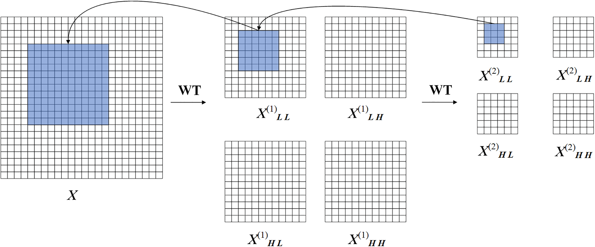
Figure 8: Convolutional diagram in the wavelet domain
The inverse wavelet transform (IWT) is the inverse process of the wavelet transform, and in the algorithm, the reconstruction of the decomposed components is achieved by transposing the convolution. Therefore, in order to obtain a higher receptive field, the WTConv downsamples the image information using a WT operation, then performs a convolution operation, and finally reconstructs the information using an IWT and outputs it, as shown in Eq. (4).
As shown in Fig. 9, by performing two WT, two IWT, and a convolution operation, a larger receptive field can be obtained with a smaller convolution kernel, which enhances the model’s focus on low-frequency information. At the same time, the algorithm can filter out some high-frequency noise, improving the model’s anti-interference ability.
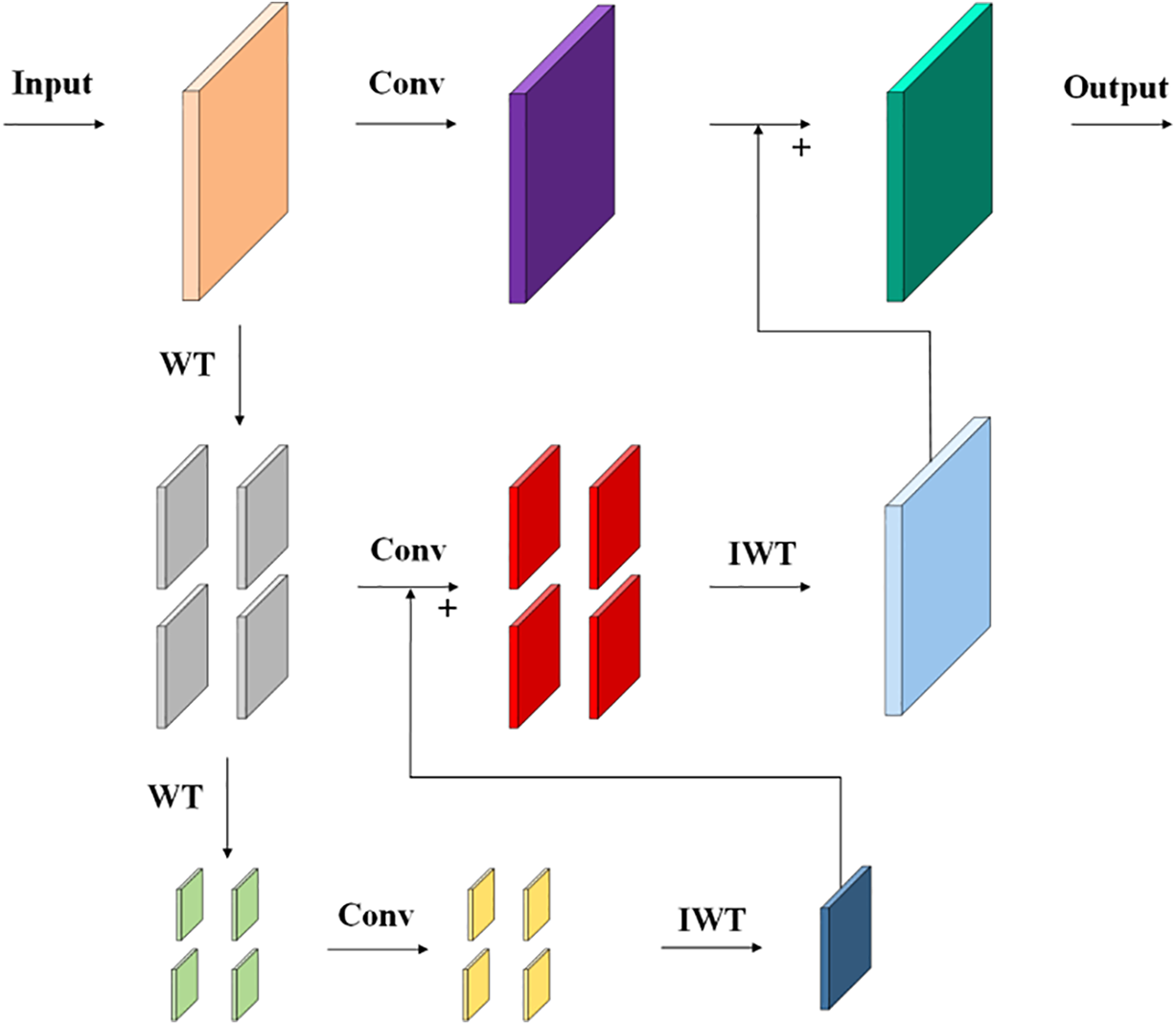
Figure 9: WTConv operating schematic
3.4 Multi-Scale Fusion and Diffusion Network
YOLOv11 retains the FPN and PAN architectures in its neck structure to integrate features of varying scales. Nevertheless, the unavoidable information loss during upsampling and downsampling processes hampers the effective exchange of contextual details. To address this limitation, this study introduces a multi-scale fusion and diffusion network designed to bolster the interaction between features of different sizes, ultimately enhancing the model’s precision in detecting road defects. The architecture is illustrated in Fig. 10.
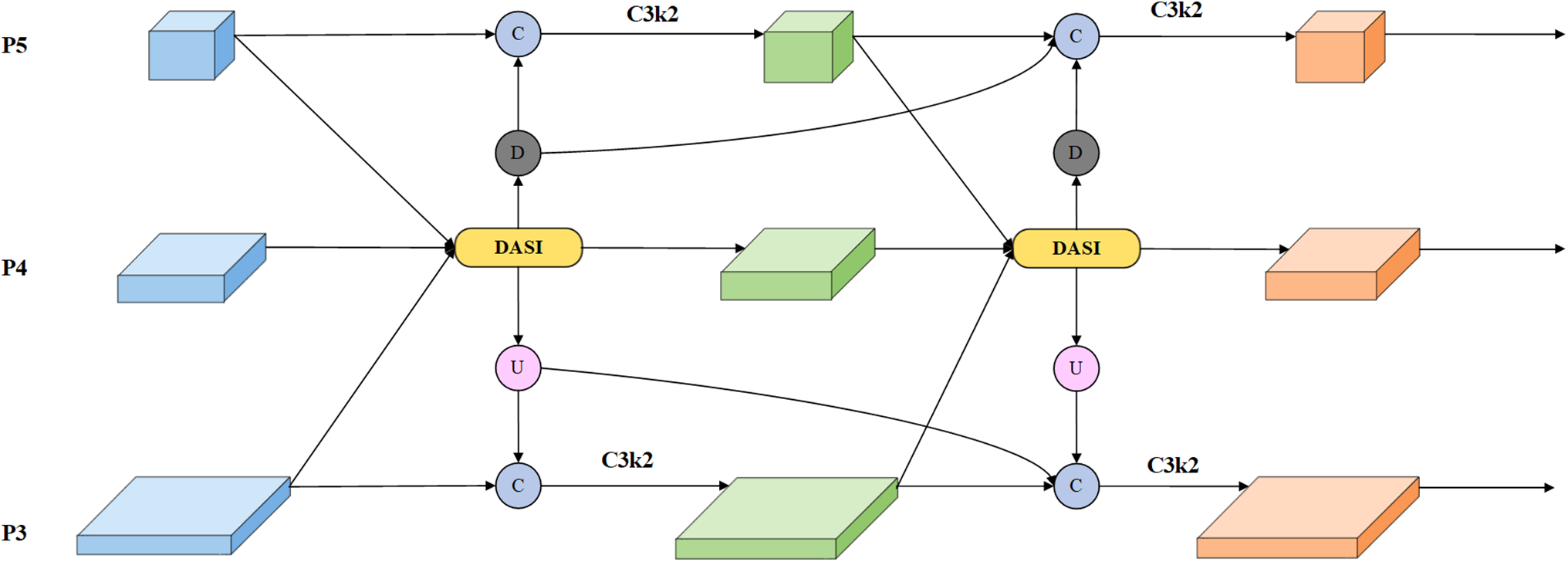
Figure 10: Multi-scale fusion and diffusion network structure diagram
The characteristics of road defects can be divided into low-dimensional features and high-dimensional features according to their location in the network. Low-dimensional features are learned in the early layers of the network and usually focus on local regional information of the data. High-dimensional features can express more complex and abstract concepts and pay more attention to contextual information. In the MFDN framework, the DASI [22] module initially combines features from various scales within the P3, P4, and P5 layers. This integrated feature data is then propagated to the P3 and P5 layers via a diffusion process. Following this, the features from the P3 and P5 layers are merged once more with the initially combined data from the P4 layer. Through this iterative fusion of features across different scales, the issue of feature degradation resulting from repeated sampling in the original neck structure is mitigated. Ultimately, the second round of fused data is diffused back to the P3 and P5 layers and combined yet again with both the original feature map and the data from the first fusion, further minimizing any loss of information. To achieve effective fusion of features of different sizes, the DASI module is used in this paper, as shown in Fig. 11. In order to achieve the fusion of different dimensional feature information, operations such as convolution and linear interpolation are used to align the high-dimensional feature
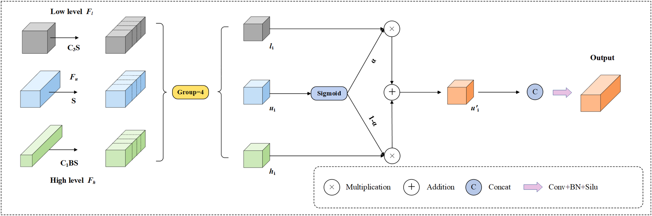
Figure 11: Structural diagram of DASI
Among them,
YOLOv11 relies on conventional striding convolutions for downsampling, a method that can sometimes overlook finer details in defects due to its inherent limitations. To address this issue, this study proposes the use of Adown as a replacement for traditional convolutions during downsampling. Adown not only bolsters the model’s ability to extract features but also trims down the overall parameter count, making the system more efficient.
As illustrated in Fig. 12, the input feature map undergoes initial smoothing via average pooling. This refined feature map is then divided into two segments along the channel dimension. The first segment is processed using a standard strided convolution for downsampling, while the second segment employs max pooling to eliminate unnecessary noise and redundant data. Following this, the channel count is fine-tuned using point-by-point convolution. Ultimately, the two segments are merged along the channel dimension, resulting in a downsampled output feature map that retains critical structural information. Adown uses different downsampling methods simultaneously through branches, and the final output feature map retains more feature information, while maximizing the retention of valid information and reducing the number of parameters and calculation of the model.
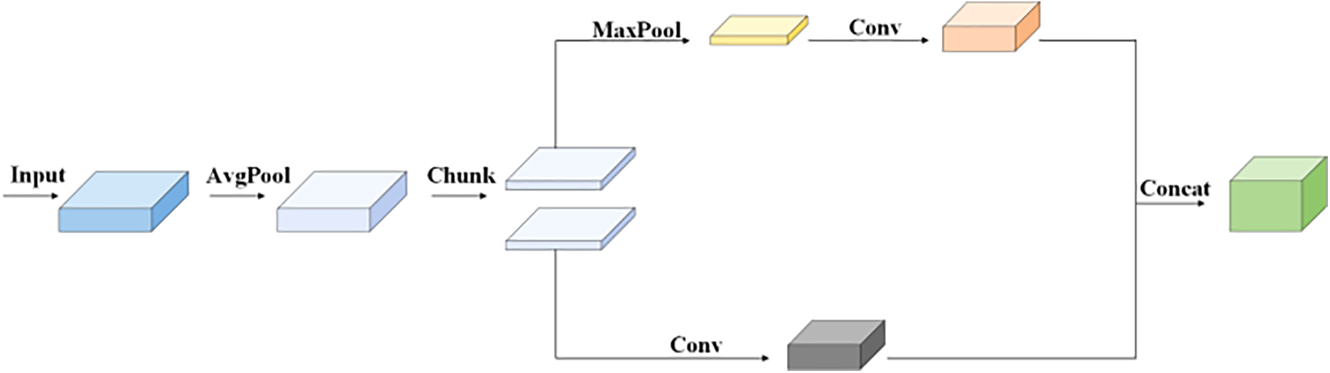
Figure 12: Structural diagram of ADown
In YOLOv11, the CIoU serves as the bounding box loss function, cleverly incorporating the aspect ratios of both the ground truth and predicted boxes, building upon the foundation of DIoU. The formula for this calculation is outlined below:
In this context, denotes the overlap ratio between the actual and predicted frames, while
Among them,
where
Among them,
4.1 Datasets and Experimental Environment
This research makes use of the RDD2022 open-source dataset, which is a goldmine of images showing road defects. The dataset includes pictures taken by in-vehicle cameras and drones, closely replicating real-life situations for detecting road defects. This, in turn, beefs up the model’s capacity to work well in different scenarios. The paper zeroes in on several kinds of road defects: D00 (longitudinal cracks), D10 (transverse cracks), D20 (mesh cracks), and Repair (road repair). For the experimental analysis, a grand total of 4373 images of Chinese roads were picked. These images were then divided into training, validation, and test sets in an 80:10:10 ratio. Some of the samples in the dataset are shown in Fig. 13. In this paper, traditional feature selection is not used, but automatic feature extraction is carried out through the modeling framework. The data processing aspect is mainly using YOLOv11’s logo data processing process, isometric scaling of the data, linear interpolation, etc., to ensure that the size of the input image is the same, and subsequent normalization.
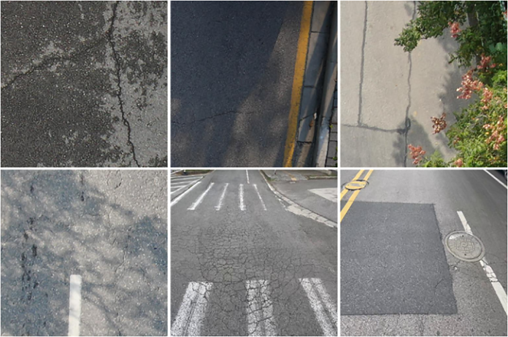
Figure 13: Example of a dataset image
To make sure the experiment is on the up-and-up, all the experiments in this paper, apart from the embedded deployment experiment, are carried out in the same experimental setup with the same configuration parameters. The experiments described in this paper were run on a server that has Ubuntu 22.04 as its operating system. The details of the specific experimental environment are laid out in Table 1, and the experimental parameters are listed in Table 2.
To comprehensively validate the efficacy of the algorithm proposed in this paper for road defect detection, multiple metrics are employed, including the F1 score, the number of floating-point operations per billion (GFLOPs), and the mean average precision of all classes at an IoU threshold of 0.5 (mAP@50%). The corresponding formulas are presented as follows:
where P denotes accuracy and R represents recall, the F1 score is the reconciled mean of P and R, a summed consideration of accuracy and recall. AP is the area under the PR curve for a single category, and mAP is a combined consideration for all the categories and is the main evaluation metric of the detection algorithm.
5.1 Loss Function Comparison Experiment
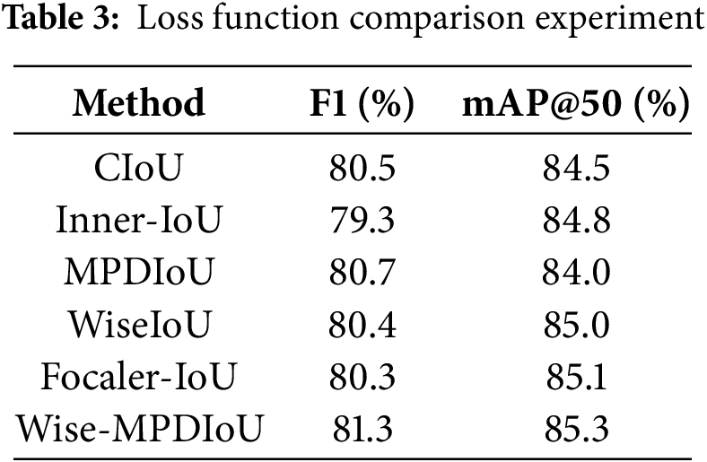
To further substantiate the benefits of Wise-MPDIoU relative to other loss functions, this study undertakes a comprehensive examination of several alternatives as a control group, including CIoU, inner-iou [23], MPDIoU, WiseIoU, and focaler_iou [24]. All experiments are conducted using the YOLOv11 benchmark model, with detailed results presented in Table 3. As indicated in Table 3, the Wise-MPDIoU loss function demonstrates superiority over its counterparts, as evidenced by enhancements in both the F1 score and mAP. Specifically, when compared to the benchmark loss function, the F1 score exhibits an improvement of 0.8%, while mAP@50% sees an increase of 0.8, leading to a notable enhancement in the algorithm’s efficacy for road defect detection.
To thoroughly evaluate how each enhancement module influences the model’s overall performance, this study carries out ablation experiments. The findings from these experiments are detailed in Tables 4–6.
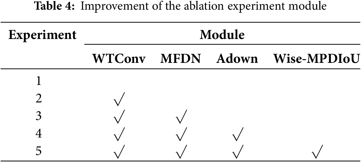
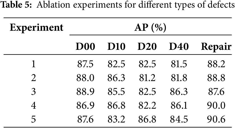
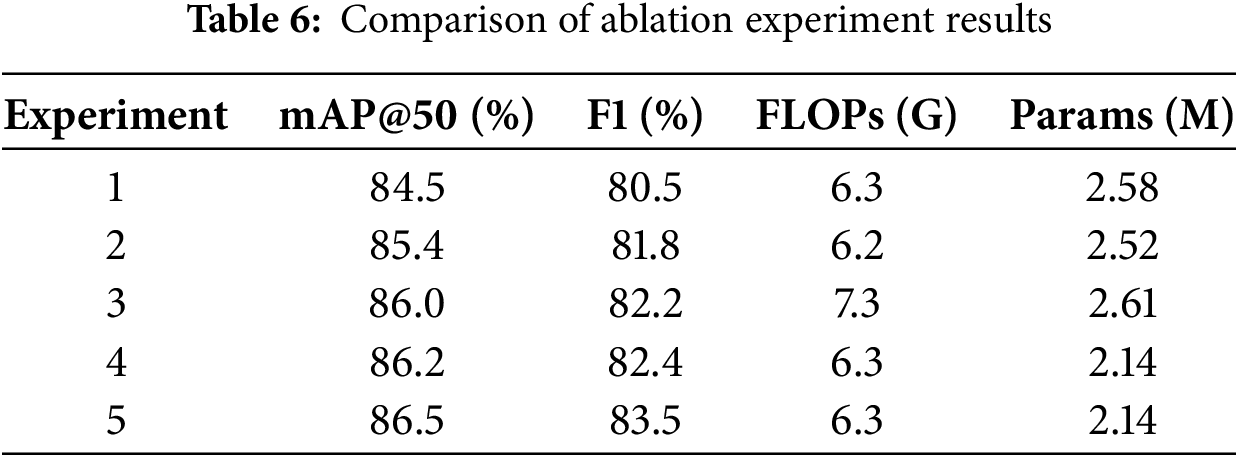
As can be seen from Table 4, experiment 1 represents the baseline model without using the improved module, experiment 2 represents the model after adding WTConv to the baseline model, experiment 3 uses the MFDN module on top of the previous experiments, experiment 4 continues on experiment 3 by replacing the global downsampling module with Adown, and experiment 5 continues on experiment 4 by adding Wise-MPDIoU, which represents the paper’s final algorithm. As can be seen from Table 5, the algorithm in this paper improves the accuracy of each type of road defect compared to the benchmark algorithm. As can be seen from Table 6, Experiment 2, after adding WTConv, the algorithm’s mAP@50% improved by 0.9%, the F1 score improved by 1.3%, and there was a small decrease in the number of model parameters and computation. Experiment 3 after using MFDN, the algorithm mAP@50% continued to improve by 0.6%, the F1 score improved by 0.4%, and there was a partial rise in the number of model parameters and computation. Experiment 4 continues with the addition of the Adown module, although the model’s mAP@50% and F1 score only improved by 0.2%, but the number of algorithmic parameters and the amount of computation has been reduced, and there has been a 17% reduction in the number of model parameters compared to the baseline. In the final experiment 5 after using the Wise-MPDIoU loss, the algorithm mAP@50% improved by 0.3%, the F1 score improved by 1.1%, the final algorithm improved by 2.0% compared to the benchmark algorithm mAP, the F1 score improved by 3.0%, and the parameter quantity has been reduced by 17%. The optimized algorithm enhances road defect detection accuracy and decreases parameter count, improving it better suited for embedded device implementation.
5.3 Comparison Experiment of Different Target Detection Algorithms
In order to more comprehensively evaluate the advantages of this algorithm over other object detection algorithms of the same scale, this paper compares this algorithm with YOLOv3-tiny, YOLOv5n, YOLO-7tiny, YOLOv8n, YOLO-9tiny, YOLO10n, and the benchmark model YOLOv11n on the RDD2022 dataset. The comparison results are shown in Table 7.
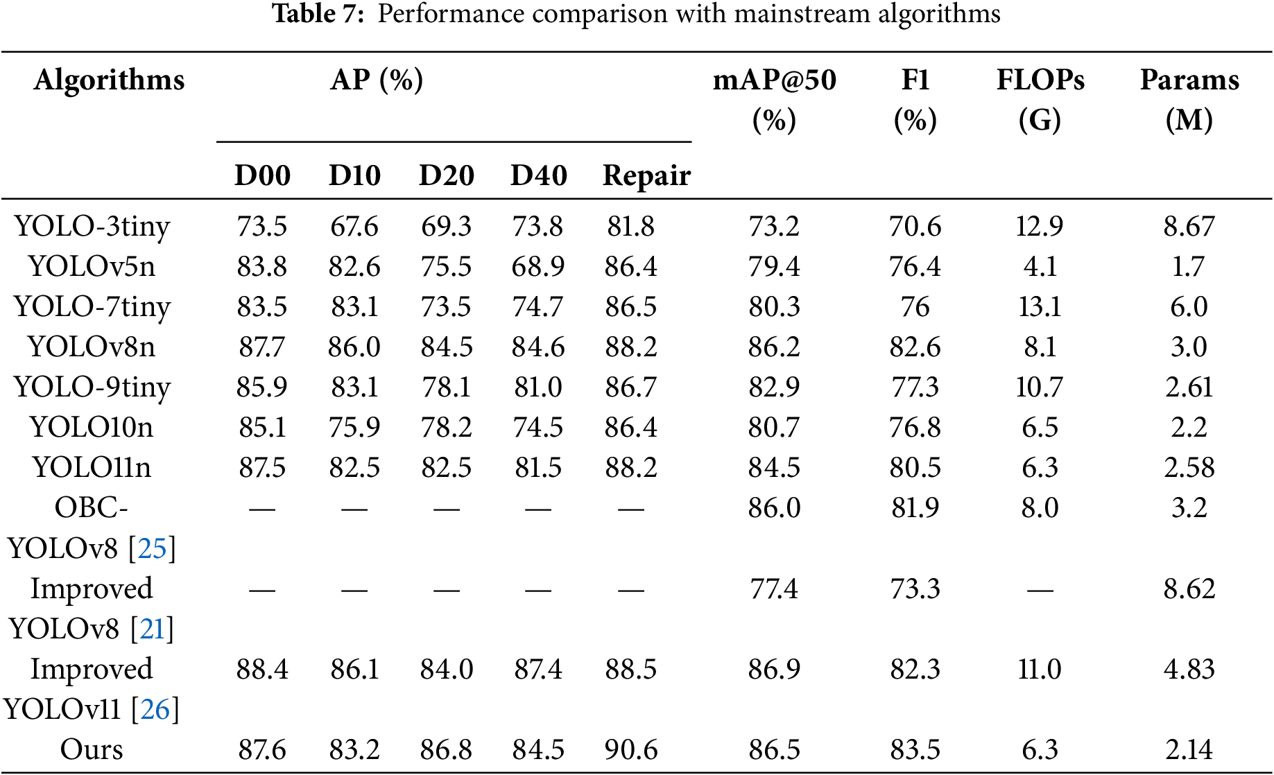
Although the detection accuracy of YOLOv11n is lower than that of YOLOv8n in the dataset used in this paper, the advantage of YOLOv11n is more obvious in terms of computational volume and the number of parameters, and the research goal of this paper is not purely to pursue the detection accuracy, which synthesizes the consideration of computational cost and detection accuracy. Secondly, YOLOv11 is the latest version in 2024, and choosing YOLOv11 as the benchmark can ensure the cutting-edge and sustainability of the research. In summary, YOLOv11n is chosen as the benchmark model in this paper. The algorithm achieves an mAP@50% of 86.5%, with an F1 score of 83.5%, which is the highest among all algorithms, proving that the algorithm has high detection accuracy in road defect detection. The algorithm’s computational complexity and parameters stand at 6.3 GFLOPs and 2.14 million, placing it slightly above YOLOv5n but beneath the majority of other object detection methods. Nonetheless, when evaluated on computational accuracy, this algorithm outperforms YOLOv5n by a considerable margin. In summary, the present algorithm demonstrates superior computational efficiency compared to its counterparts, making it particularly adept for detecting road defects. At the same time, this paper adds the comparison experiments on the research results of other researchers, also in the part of the RDD2022 Chinese dataset, OBC-YOLOv8 and Improved YOLOv8 have a certain gap with this paper’s model in terms of the computational accuracy and computational scale, and the Improved YOLOv11, although it has a little advantage in terms of the detection accuracy, is almost twice as good as the present paper’s algorithm in terms of the computational volume and the number of parameter part. Algorithm is twice as much as the algorithm of this paper, and the comprehensive performance is better. However, it is almost twice as much as this paper’s algorithm in the calculation amount and parameter part, with better comprehensive performance.
To better demonstrate the algorithm’s enhanced capability in identifying road defects, we performed visual comparisons with alternative algorithms from three distinct viewpoints: (a) images captured from a motorcycle showcasing various defect types, (b) aerial images displaying multiple defects, and (c) images of defects obscured by shadows, as depicted in Fig. 14. In the first comparison (a), our algorithm achieved the highest average confidence for defect detection while exhibiting neither false positives nor missed detections. In the second comparison (b), aside from our algorithm and YOLOv9-tiny, all other algorithms exhibited varying degrees of false detections and missed detections, whereas our approach maintained a higher confidence level. Lastly, in the shadowed defect comparison (c), our algorithm demonstrated notable confidence and proved to be the least affected by shaded areas.
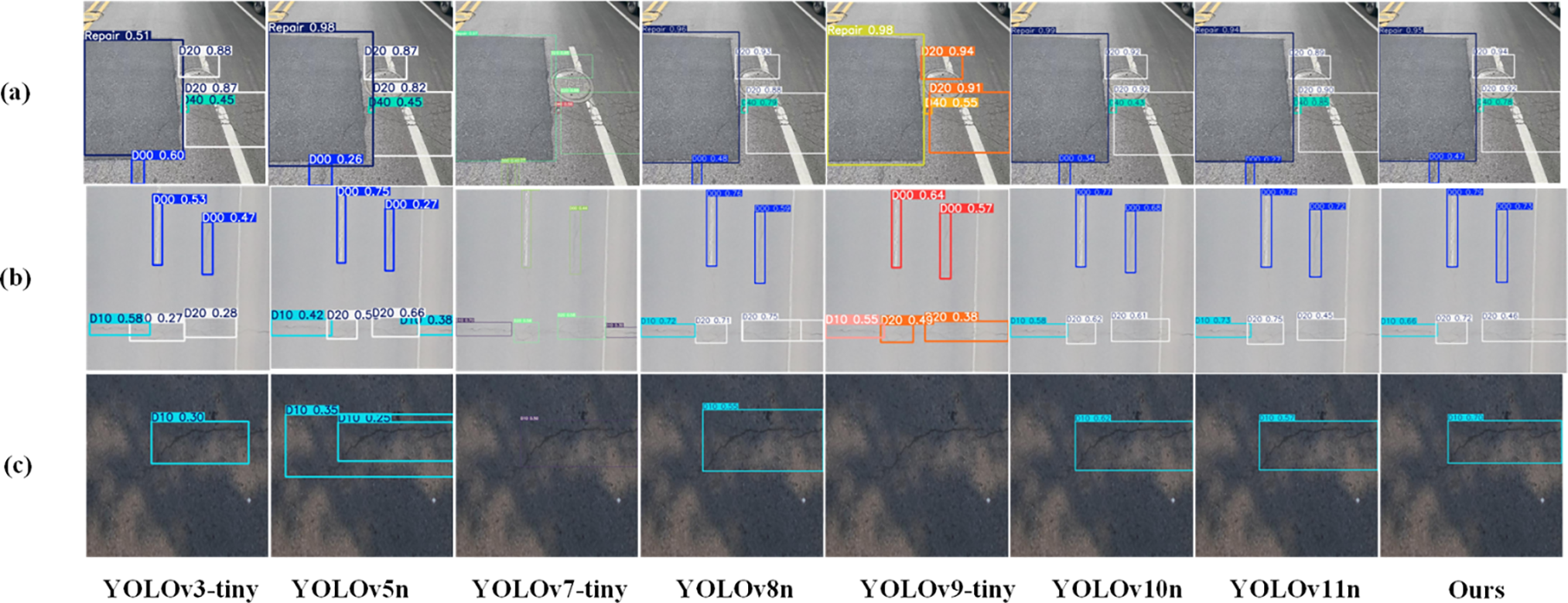
Figure 14: Visual comparison with mainstream algorithms
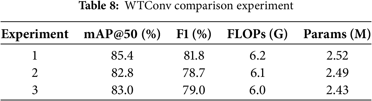
WTConv allows the model to focus more on low-frequency information, the main role of the neck network is to fuse different scales of information, and the excessive use of the neck network may lead to the loss of high-frequency information. Due to the fact that road defect images have many complex targets, including small cracks and composite damages, the loss of high-frequency information may lead to inaccurate target localization or even miss detection and misdetection. In order to verify the detection effect of WTConv in the model, this paper designs a comparison experiment, experiment 1 replaces the part of the backbone network, experiment 2 replaces the part of the neck network, and experiment 3 replaces all. As can be seen from Table 8, adding WTConv to the backbone network only provides a better balance of accuracy and computational cost, with more obvious advantages over experiments 2 and 3.
5.5 Multi-Country Road Defect Generalization Experiment
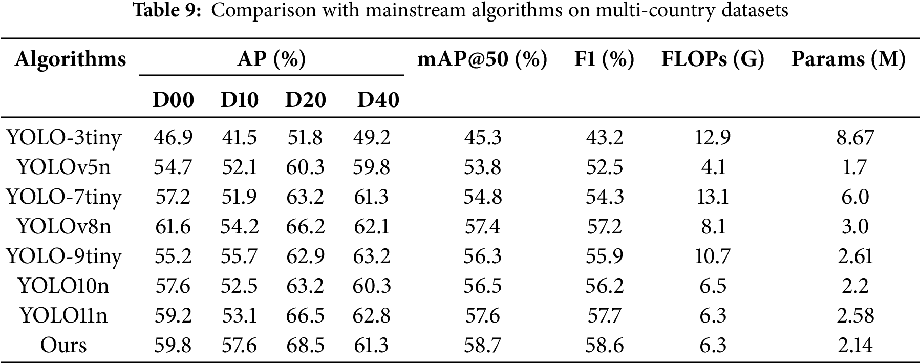
In order to evaluate the performance of the algorithm on road defects detection more comprehensively, this paper combines road defects data from Japan, Czech Republic, United States, and India, and obtains 17,000 images after retaining the common categories and filtering out the untargeted data, which are divided into a training set, a validation set, and a test set in accordance with 8:1:1 for training. The experimental results are shown in Table 9, and it can be concluded that the algorithm of this paper still has better comprehensive performance in road defect data containing more countries.
5.6 Embedded Device Deployment Experiment
To assess the practical effectiveness of the algorithm discussed in this paper, it has been implemented on the Raspberry Pi 4B embedded device. The relevant specifications are detailed in Table 10. The Raspberry Pi is popular for its affordability and energy efficiency, making it an ideal platform for evaluating the algorithm’s performance in real-world applications. The baseline model YOLOv11n and the algorithm discussed in this study were implemented on a Raspberry Pi, with the experimental outcomes illustrated in Fig. 15. The results reveal that the proposed algorithm achieved neither false positives nor missed detections. When compared to the baseline model, this algorithm demonstrates a higher detection confidence, signifying improved accuracy in identifying road defects. In the upper left corner of the image, the FPS is displayed. Given the Raspberry Pi’s resource constraints, the detection speed is relatively modest. Nonetheless, it is evident that the detection speeds for both the proposed algorithm and the baseline model are quite similar, hovering around 0.57. As the newest entry in the YOLO series, YOLOv11 is distinguished by its excellent detection speed and adaptability for deployment. Consequently, the detection speed achieved by the algorithm in this study satisfies the criteria for real-time detection, and with its superior accuracy and reduced parameter count, it is particularly well-suited for integration into embedded systems.
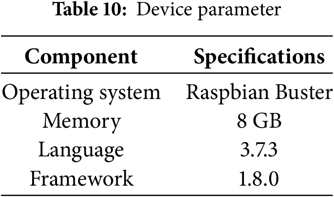
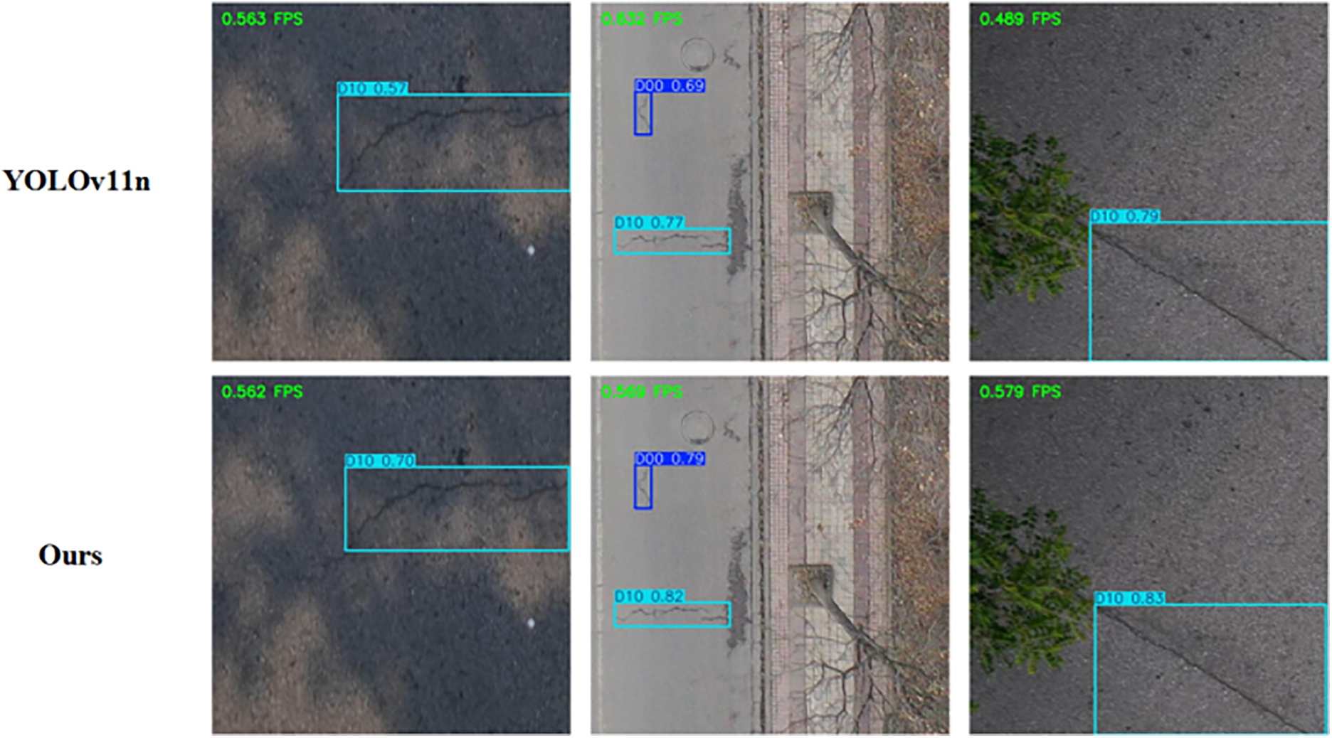
Figure 15: Comparison of embedded deployment results
Although the algorithm in this paper has achieved effective improvement in road defect detection, it still has certain limitations: although the algorithm in this paper achieves real-time performance on embedded devices, it may still be insufficient in actual detection, and subsequent consideration will be given to improving the detection speed through further optimization of the algorithm. The detection ability of the dataset in the face of rare or composite defects needs to be examined, and subsequent work will further expand the dataset or improve the generality of the model through data enhancement.
Given the issues of low accuracy, false positives, and missed detections in current road defect detection algorithms, this paper introduces a novel method based on YOLOv11. Key components of the proposed algorithm include C3K2_WTConv, MFDN, ADown, and Wise-MPDIoU. We conducted a series of comparative and ablation studies using the RDD2022 dataset, as well as tests on the Raspberry Pi embedded device. The results from these experiments highlight the algorithm’s effectiveness in enhancing road defect detection precision, achieving an mAP of 86.5%. Additionally, the approach significantly decreases the number of model parameters, making it feasible to deploy on devices constrained by resources. The findings reinforce the algorithm’s practical viability, showcasing its potential for real-world implementation. Future work focuses on further compressing the model size through knowledge distillation or pruning to improve the inference speed and enhance the practical value of the model for road inspection in real-world environments.
Acknowledgement: Thank the reviewers for their valuable comments on this article.
Funding Statement: The authors received no specific funding for this study.
Author Contributions: The authors’ contributions to this paper are as follows: Research ideas and direction design: Xubo Liu, Yunxiang Liu, Peng Luo; Data processing: Xubo Liu, Yunxiang Liu; The experiment was conducted: Xubo Liu, Yunxiang Liu, Peng Luo; Statistical summary: Yunxiang Liu, Peng Luo; Embedded device experiment: Xubo Liu; Thesis writing: Xubo Liu. All authors reviewed the results and approved the final version of the manuscript.
Availability of Data and Materials: The data that support the findings of this study are openly available at https://github.com/sekilab/RoadDamageDetector (accessed on 20 June 2025).
Ethics Approval: Not applicable.
Conflicts of Interest: The authors declare no conflicts of interest to report regarding the present study.
References
1. Yang X, Zhang J, Liu W, Jing J, Zheng H, Xu W. Automation in road distress detection, diagnosis and treatment. J Road Eng. 2024;4(1):1–26. doi:10.1016/j.jreng.2024.01.005. [Google Scholar] [CrossRef]
2. Khan MAA, Alsawwaf M, Arab B, AlHashim M, Almashharawi F, Hakami O, et al. Road damages detection and classification using deep learning and UAVs. In: Proceedings of the 2022 2nd Asian Conference on Innovation in Technology (ASIANCON); 2022 Aug 26–28; Ravet, India. Piscataway, NJ, USA: IEEE; 2022. p. 1–6. doi:10.1109/ASIANCON55314.2022.9909043. [Google Scholar] [CrossRef]
3. Finder SE, Amoyal R, Treister E. Wavelet convolutions for large receptive fields. In: Proceedings of the European Conference on Computer Vision (ECCV); 2024 Sep 29–Oct 4; Milan, Italy. Cham, Switzerland: Springer Nature; 2024. p. 363–80. [Google Scholar]
4. Wang CY, Yeh IH, Mark Liao HY. YOLOv9: learning what you want to learn using programmable gradient information. In: Proceedings of the Computer Vision—ECCV 2024; 2024 Sep 29–Oct 4; Milan, Italy. Cham, Switzerland: Springer Nature; 2024. p. 1–21. doi:10.1007/978-3-031-72751-1_1. [Google Scholar] [CrossRef]
5. Tong ZJ. Wise-IoU: bounding box regression loss with dynamic focusing mechanism. arXiv:2301.10051. 2023. [Google Scholar]
6. Ma SL, Yong X. MPDIoU: a loss for efficient and accurate bounding box regression. arXiv:2307.07662. 2023. [Google Scholar]
7. Girshick R. Fast R-CNN. In: Proceedings of the 2015 IEEE International Conference on Computer Vision (ICCV); 2015 Dec 7–13; Santiago, Chile. Piscataway, NJ, USA: IEEE; 2015. p. 1440–8. doi:10.1109/ICCV.2015.169. [Google Scholar] [CrossRef]
8. Ren S, He K, Girshick R, Sun J. Faster R-CNN: towards real-time object detection with region proposal networks. IEEE Trans Pattern Anal Mach Intell. 2017;39(6):1137–49. doi:10.1109/tpami.2016.2577031. [Google Scholar] [PubMed] [CrossRef]
9. He K, Gkioxari G, Dollár P, Girshick R. Mask R-CNN. In: Proceedings of the 2017 IEEE International Conference on Computer Vision (ICCV); 2017 Oct 22–29; Venice, Italy. Piscataway, NJ, USA: IEEE; 2017. p. 2980–8. doi:10.1109/ICCV.2017.322. [Google Scholar] [CrossRef]
10. Cai Z, Vasconcelos N. Cascade R-CNN: high quality object detection and instance segmentation. IEEE Trans Pattern Anal Mach Intell. 2021;43(5):1483–98. doi:10.1109/TPAMI.2019.2956516. [Google Scholar] [PubMed] [CrossRef]
11. He K, Zhang X, Ren S, Sun J. Spatial pyramid pooling in deep convolutional networks for visual recognition. IEEE Trans Pattern Anal Mach Intell. 2015;37(9):1904–16. doi:10.1109/tpami.2015.2389824. [Google Scholar] [PubMed] [CrossRef]
12. Li Q, Xu X, Guan J, Yang H. The improvement of faster-RCNN crack recognition model and parameters based on attention mechanism. Symmetry. 2024;16(8):1027. doi:10.3390/sym16081027. [Google Scholar] [CrossRef]
13. Tang J, Mao Y, Wang J, Wang L. Multi-task enhanced dam crack image detection based on faster R-CNN. In: Proceedings of the 2019 IEEE 4th International Conference on Image, Vision and Computing (ICIVC); 2019 Jul 5–7; Xiamen, China. Piscataway, NJ, USA: IEEE; 2019. p. 336–40. doi:10.1109/icivc47709.2019.8981093. [Google Scholar] [CrossRef]
14. Chen Q, Gan X, Huang W, Feng J, Shim H. Road damage detection and classification using mask R-CNN with DenseNet backbone. Comput Mater Contin. 2020;65(3):2201–15. doi:10.32604/cmc.2020.011191. [Google Scholar] [CrossRef]
15. Chen L, An S, Zhao S, Li G. MS-FPN-based pavement defect identification algorithm. IEEE Access. 2023;11(20):124797–807. doi:10.1109/access.2023.3329250. [Google Scholar] [CrossRef]
16. Li P, Sun L, Xie Z, Shan J. Road crack image detection algorithm based on improved MobileNet-SSD. Laser J. 2022;43(7):123–7. [Google Scholar]
17. Liu C, Yao Y, Li J, Qian J, Liu L. Research on lightweight GPR road surface disease image recognition and data expansion algorithm based on YOLO and GAN. Case Stud Constr Mater. 2024;20(13):e02779. doi:10.1016/j.cscm.2023.e02779. [Google Scholar] [CrossRef]
18. Roy AM, Bhaduri J. DenseSPH-YOLOv5: an automated damage detection model based on DenseNet and Swin-Transformer prediction head-enabled YOLOv5 with attention mechanism. Adv Eng Inf. 2023;56(12):102007. doi:10.1016/j.aei.2023.102007. [Google Scholar] [CrossRef]
19. Wan F, Sun C, He H, Lei G, Xu L, Xiao T. YOLO-LRDD: a lightweight method for road damage detection based on improved YOLOv5s. EURASIP J Adv Signal Process. 2022;2022(1):98. doi:10.1186/s13634-022-00931-x. [Google Scholar] [CrossRef]
20. Chen J, Zou C, Wang S, Xia L, Chen Z. Research on rapid detection method of pavement defects by improving YOLOv5. Electron Meas Technol. 2023;46(10):129–35. [Google Scholar]
21. Sun Z, Zhu L, Qin S, Yu Y, Ju R, Li Q. Road surface defect detection algorithm based on YOLOv8. Electronics. 2024;13(12):2413. doi:10.3390/electronics13122413. [Google Scholar] [CrossRef]
22. Xu S, Zheng S, Xu W, Xu R, Wang C, Zhang J, et al. HCF-Net: hierarchical context fusion network for infrared small object detection. In: Proceedings of the 2024 IEEE International Conference on Multimedia and Expo (ICME); 2024 Jul 15–19; Niagra Falls, ON, Canada. Piscataway, NJ, USA: IEEE; 2024. p. 1–6. [Google Scholar]
23. Zhang H, Xu C, Zhang S. Inner-IoU: more effective intersection over union loss with auxiliary bounding box. arXiv:2311.02877. 2023. [Google Scholar]
24. Zhang H, Zhang S. Focaler-IoU: more focused intersection over union loss. arXiv:2401.10525. 2024. [Google Scholar]
25. Zhang S, Liu Z, Wang K, Huang W, Li P. OBC-YOLOv8: an improved road damage detection model based on YOLOv8. PeerJ Comput Sci. 2025;11(11):e2593. doi:10.7717/peerj-cs.2593. [Google Scholar] [PubMed] [CrossRef]
26. Luo Z, Jiang Y, Li W. A road defect detection model based on improved YOLOv11n. Microelectron Comput. 2025;1:1–13. [cited 2025 May 10]. Available from: https://link.cnki.net/urlid/61.1123.TN.20250225.1018.010. [Google Scholar]
Cite This Article
 Copyright © 2025 The Author(s). Published by Tech Science Press.
This work is licensed under a Creative Commons Attribution 4.0 International License , which permits unrestricted use, distribution, and reproduction in any medium, provided the original work is properly cited.
 Downloads
 Citation Tools