
 Submit a Paper
 Propose a Special lssue
 Open Access
REVIEW

From Spatial Domain to Patch-Based Models: A Comprehensive Review and Comparison of Multimodal Medical Image Denoising Algorithms
1 University School of Computing, Sunstone, Rayat Bahra University, Mohali, 140104, Punjab, India
2 Chitkara University Institute of Engineering & Technology, Chitkara University, Rajpura, 140401, Punjab, India
3 Marwadi University Research Centre, Department of Engineering, Marwadi University, Rajkot, 360003, Gujarat, India
* Corresponding Author: Ayush Dogra. Email:
Computers, Materials & Continua 2025, 85(1), 367-481. https://doi.org/10.32604/cmc.2025.066481
Received 09 April 2025; Accepted 26 July 2025; Issue published 29 August 2025
 View Full Text
 Download PDF
Abstract
To enable proper diagnosis of a patient, medical images must demonstrate no presence of noise and artifacts. The major hurdle lies in acquiring these images in such a manner that extraneous variables, causing distortions in the form of noise and artifacts, are kept to a bare minimum. The unexpected change realized during the acquisition process specifically attacks the integrity of the image’s quality, while indirectly attacking the effectiveness of the diagnostic process. It is thus crucial that this is attended to with maximum efficiency at the level of pertinent expertise. The solution to these challenges presents a complex dilemma at the acquisition stage, where image processing techniques must be adopted. The necessity of this mandatory image pre-processing step underpins the implementation of traditional state-of-the-art methods to create functional and robust denoising or recovery devices. This article hereby provides an extensive systematic review of the above techniques, with the purpose of presenting a systematic evaluation of their effect on medical images under three different distributions of noise, i.e., Gaussian, Poisson, and Rician. A thorough analysis of these methods is conducted using eight evaluation parameters to highlight the unique features of each method. The covered denoising methods are essential in actual clinical scenarios where the preservation of anatomical details is crucial for accurate and safe diagnosis, such as tumor detection in MRI and vascular imaging in CT.Keywords
A denoising technique’s primary job is to minimize the background noise and, thus, enhance image quality for better visualization and diagnosis via better feature extraction and object recognition. Denoising can be considered a preliminary process before the final image is delivered. However, a significant limitation of denoising is the trade-off between reducing noise and preserving critical anatomical landmarks. In natural images, the noise induced by camera sensors is neither additive nor uniform over different grey levels [1]. The case of medical imaging is different from that of natural imaging in the sense that in medical imaging, the noises are signal-dependent with surfaces that are impossible to miss, making it hard for the conventional denoising techniques to remove them. The aftermaths of applying various spatially variant, direction-sensitive transformations to these images may result in further degradation if the process is not monitored and appropriately controlled. The nature of the image is affected by the nature and proximity of noise, making it very difficult to extract meaningful information, structures, and subtle elements from the debased image, vital for the diagnostic process [2].
Many imaging modalities exist in the medical field, of which CT and MRI imaging are the two most common and most popularly used. As the trend toward laboratory tests faded over time, the diagnosis process through images took over due to its efficiency and effectiveness. Some of the imaging techniques also provide results in real time. However, some challenges remained in the form of sensor noises or other environmental noises, along with artifacts. For the image to be clear, it must have a high signal-to-noise ratio (SNR), and these modalities can provide excellent results if all the prerequisites are achieved with utmost care. Nevertheless, if these pre-requisites are not addressed appropriately, the images may turn out to be noisy and of no use at all [2–6].
Real-world challenges such as time constraints for processing, computational resource limitations, and the need for seamless integration into existing diagnostic processes sometimes constrain the application of denoising techniques in clinical practice. High-throughput environments, e.g., radiology departments or emergency rooms, require fast image processing without compromising diagnostic accuracy. In addition, not every clinical environment will possess the memory and processing power required by some advanced algorithms, deep learning models. These limitations emphasize the importance of developing useful and adaptable denoising methods.
Multimodal denoising methods that combine complementary data from multiple spaces—spatial, frequency, and learned feature spaces—have been increasingly recognized as a response to these challenges. Multimodal techniques can capitalize on numerous strengths to better preserve noise elimination with clinically important features, whereas single-domain approaches may be vulnerable to complex patterns of noise or modality-based distortion. Consequently, this study emphasizes the necessity and growing relevance of hybrid and multimodal denoising models that are tailored to the pragmatic needs of real-world medical imaging environments.
Challenges in Medical Image Denoising:
Medical image denoising has a unique and more challenging problem set than natural image denoising, which has been well researched. Medical images are characterized by highly specific anatomical and pathological features, which have to be preserved with the utmost precision for an effective diagnosis, unlike natural images, which may contain broad and redundant structures at times. Clinical expertise can be compromised if even minor structural features get lost in denoising.
In addition, in comparison to natural image sensors, noise characteristics specific to sensors in medical imaging devices (e.g., CT, MRI, and PET) are often more complex and varied. An example includes the non-stationary, non-Gaussian nature of MRI images, which are prone to Rician noise, and CT scans, which are often affected by Poisson noise.
Because of privacy, ethical, and cost concerns, there is a lack of extensive, annotated training data for medical images, another key difference. The existence of vast datasets in the natural picture domain is the complete opposite. In addition, clinical constraints such as low-dose imaging (to reduce radiation exposure) lead to inherently noisier images, so effective denoising is harder. Because of privacy, ethical, and cost concerns, there is a lack of large, annotated training data for medical images, which is another key difference. The existence of huge datasets in the natural image world is in direct contrast to this. In addition, clinical constraints such as low-dose imaging (to reduce radiation) yield naturally noisier images, rendering effective denoising more difficult.
Finally, the structural preservation and diagnostic integrity need to be taken most seriously in medical image denoising, unlike natural images, where perceptual quality is often sufficient. In a clinical environment, where deceptive features can lead to misdiagnosis, oversmoothing or hallucinating details techniques that are permissible in natural picture improvement are not suitable. Because of such issues, denoising medical images is not merely a technology problem but an area that necessitates a tremendous level of inter-disciplinary perception that combines experience of medical imaging modalities and clinical relevance along with expertise of image processing.
As compared to existing literature, this paper presents a comprehensive and comparative study of 80 denoising algorithms covering the three principal distributions of noise (Gaussian, Poisson, and Rician). This paper is a more practical guide for researchers and industries as it systematically ranks performance based on eight specified evaluation measures, as opposed to existing surveys that only focus on algorithmic concepts. The research also proposes issues specific to every modality and recommends an organization of denoising algorithms based on areas of application (spatial, transform, and sparse). Further, it presents clinical constraints like computational expense and time, and data diversity and angle dependency on PSNR as issues that have often been neglected in past analyses.
Additionally, imaging through these modalities is expensive, posing another challenge. These reasons push forward the case of the need for image refinement solutions through image processing. Fortunately, due to advancements in image processing, there are plenty of tools available. However, research will improve these techniques and make them suitable specifically for processing medical images. The trend also indicates the rise in popularity of image processing tools for medical images as the number of publications increased drastically in recent years (Fig. 1) [7–10].
Figure 1: Number of publications published with keywords or title CT denoising and MRI denoising from 2009 to 2023 (Source: Google Scholar)
Therefore, putting forth three crucial arguments in favour of the need for a workable denoising technique:
1. A low-resolution (LR) medical image can be converted into a high-resolution (HR) image without repeating the scan with denoising’s help. This is particularly important in cases where rescanning is not feasible or poses a risk to the patient’s health. Additionally, denoising can improve the accuracy of medical image analysis by reducing the impact of noise on image features and patterns. This is especially important in fields such as radiology and pathology, where accurate interpretation of medical images is critical for diagnosis and treatment planning. Finally, denoising can help reduce radiation exposure in medical imaging by allowing for lower-dose scans that still produce high-quality images.
2. By denoising and enhancing a low-radiation image, a high-quality image can be produced, reducing the need for high radiation exposure, as in a CT scan. This is particularly important for patients who require multiple scans over time, as repeated exposure to high levels of radiation can increase the risk of cancer.
3. Denoising brings forth a clearer image, reducing the time for diagnosis by medical professionals. In addition, enhanced images can reveal subtle details that may have been missed in the original scan, leading to more accurate diagnoses and better treatment plans [11,12].
The remainder of this paper is organized as follows: Section 2 provides a detailed overview of the medical imaging modalities. Section 3 categorizes and discusses traditional and advanced denoising techniques across spatial, transform, and sparse domains. In Section 4, various Thresholding methods used in denoising have been covered. Section 5 covers the image noise models and artifacts. Section 6 outlines the evaluation metrics used for performance analysis. Section 7 presents the experimental results and comparative assessments. Section 8 discusses limitations, clinical relevance, and future research directions. And concludes the paper with key findings and contributions.
2 Medical Imaging Modalities (CT and MRI)
The new era of technology heralded a revolution in medicine. As we know it today, the practice of medicine results from years of research that went into the development of modern imaging techniques. Since the discovery of the “X-Rays” in 1895, the domain of imaging in medicine has grown by leaps and bounds. As the understanding of these rays grew, it had significant implications for medical imaging. During the period between the discovery of X-rays by Roentgen and the invention of CT scans in 1972 by Hounsfield, the field of medical imaging evolved at a slow pace. The change came with the development of the CT device. It changed how we saw the human body. The X-Ray generated a black-and-white image, in which it was challenging for a clinician to demarcate various body parts. The CT device transmitted the X-Rays simultaneously, measuring the degree of the attenuation coefficient of different tissues to the X-Rays [11]. With the CT came the “Hounsfield Scale,” a quantitative grayscale for describing the human body parts’ radio density. Thus, it increased our potential for visualization of the human body as it was more sensitive than the conventional X-Ray systems. This increased screening, diagnostic, and monitoring capabilities also helped us understand the human anatomy more clearly. However, the recent advances in technology have focused on improving the quality of images produced by these modalities [12]. Medical imaging has made significant progress in giving precise and thorough information about the human body with the development of new technologies. The development of CT scans and MRI devices changed radiology by enabling the study of inside organs and tissues to be seen in greater detail. Healthcare workers may now identify and diagnose illnesses at an earlier stage thanks to these modalities, which have shown to be more sensitive than traditional X-ray systems. Also, they have aided in tracking the development of illnesses and gauging the success of therapies. The quality of the pictures generated by these modalities has been further enhanced by recent technological developments, increasing their usefulness in medical diagnosis and treatment planning. We may anticipate even more advanced imaging technologies as a result of ongoing research and development, which will help us better comprehend the human anatomy and treat patients.
3 Conventional Denoising on Medical Images
As mentioned previously in the introduction, the noise in medical images is signal-dependent, i.e., it varies with the signal’s intensity. The majority of conventional cutting-edge techniques are ineffective in addressing this noise issue. Their inability to adapt to signal-dependent noise characteristics is the primary cause. These techniques frequently presume a fixed statistical model for noise, which may not accurately depict the complex and variable nature of noise in medical images. For instance, Coifman et al. (1995) demonstrated that a widely used denoising technique based on Gaussian assumptions performed inadequately when applied to medical images with non-Gaussian noise distributions [13]. This emphasizes the demand for more sophisticated denoising methods that can manage the various noise patterns present in medical images. For enhancing the accuracy and dependability of medical image analysis, it will be essential to create algorithms that can adapt to signal-dependent noise characteristics.
3.1 Filtering in Spatial Domain
Spatial filtering is performed by convolution of the image with a kernel capable of modifying an image in a particular way on the pixel level. In spatial domain filtering, neighbourhood operations are performed with a fixed-size array (kernel) designed to smooth, sharpen, or extract edges. The low-frequency information includes equal intensity areas. In contrast, the high-frequency information represents the intensity variations within an image. The smoothing process is equivalent to low-pass filtering, and the extraction of edges is equivalent to high-pass filtering of the image. The kernel is used to perform averaging as a neighbourhood operation on the pixels of the image to modify them spatially, i.e., the pixel under consideration is replaced with the weighted average of the pixels in its neighbourhood. This neighbourhood averaging operation can be described mathematically as [14].
Fig. 2 shows the generic process of image denoising. It shows how denoising process can be carried out. First the noise is added to source image then preprocessing like histogram equalization, noise estimation, etc. is performed on the noisy image. Then image denoising algorithms is applied and at last the denoised image is produced.
Figure 2: A generic image denoising process
Eq. (1) shows that the calculations are performed over a square window of size m
The simplest example of the neighbourhood averaging operation is box filter or mean filter. The name box filter is assigned due to its frequency response resembling a box. A simple 3
Fig. 3 shows the image denoising techniques and various its classification. The average filter possesses some properties like zero shift, i.e., the object position is not shifted after the operation due to its zero-phase, which implies a symmetric filter mask with a real-valued transfer function. It is well known that the smoothing operator affects the finer scales more than the coarser scales, which means that it should have the monotonically decreasing transfer function so that a particular scale does not get annihilated while simultaneously preserving the smaller scales. Additionally, the smoothing should be the same in all directions, i.e., it should be isotropic. In discrete spaces, this goal is hard to achieve. So, it can be seen as a potential challenge to design kernels that deviates the least from isotropy [16].
Figure 3: Denoising methods classifications
The time-domain representation or the inverse Fourier transform of this box function is a Sinc function. A filter can be represented either in IIR (Infinite Impulse Response) form or FIR (Finite Impulse Response) form. When expressed in FIR form, the time domain’s impulse response needs to be truncated, making the filter perform poorly near the edges. Due to sharp cut-offs in the frequency domain, this filter also introduces ringing near the shapes’ boundaries in the images. Another drawback of the mean filter is that a pixel with the least significance can also influence the average value of pixels in its neighbourhood, affecting the pixels’ values near edges, which leads to the loss of essential details in the image. The filter also deviates from isotropy when the mask size is increased beyond a specific limit, which leads to the decision that the choice of mask size is subjective to the data in hand [18]. In [14], authors presented effective ways in which the mean filter can be used to handle complex images and in [19], non-linear mean filters were used to denoise the medical images and detect edges for effective diagnosis.
It is possible to derive better smoothing filters by knowing the relation between the Fourier transform pairs’ compactness and the smoothness. In the case of mean/box filters where the smaller size of filter masks resulted in degraded transfer functions, the larger mask sizes improved the transfer function at the cost of increased overshoot along with compromised isotropy. The edges or intensity variations are regarded as discontinuities in space, and the Fourier transform’s envelope of a signal having discontinuities in space decays in the frequency domain. This paves the way for the synthesis of efficient filters called the Binomial filters. The 1-D Binomial filter mask can be written as [20,21]
It is the convolution of the elementary binomial smoothing mask,
These masks have values of binomial distribution hence the name Binomial filters. The transfer functions of Binomial filters are monotonically decreasing with zero value at the highest spatial frequency. As the order of the filter is increased, the transfer function tends toward Gaussian distribution. Similarly, in 2-D Binomial filters, when order is increased, the filter loses its isotropic nature. It tends towards an anisotropic character as the transfer function increases in the direction of diagonals. While these linear filters effectively deal with zero-mean Gaussian noise, they cannot appropriately tackle impulse noise [20–23].
Further improvement in mean filters came through Alpha-trimmed mean filters designed for Gaussian noise with underlying impulse noise components. This filter lies on the boundary of mean filters and median filters, where the value of
where
The linear filters are useful in the case of Gaussian noise but perform poorly in the case of binary noise. Additionally, it is generally assumed that every pixel carries information. So, in linear filtering, the information simply gets carried to the neighbouring pixels rather than elimination. The task at hand remains to identify these pixels and eliminate them. The rank-value or median filters do this task [27,28]. The non-linear filters select the medium value of intensity arranged in ascending order based on the array position [29]. As an impulse will be surrounded by the pixels of almost equal intensity, it falls on the sorted array’s extremes; hence it gets replaced with other appropriate pixels. Besides, edges and constant neighbourhoods are also preserved as they are regarded as fixed points. For a single unnecessary discontinuity, lower window sizes are used, whereas larger window sizes are used for the groups of infected pixels [30].
The median filter operation tends to remove thin corners and lines, and its performance is rather unsatisfactory in signal-dependent noise. So, the issue of MRI imaging will not be addressed effectively with this kind of filtering [31]. Later on, other more efficient median filter variants were introduced, trying to solve the associated problems by adaptive measures. The first such evolved variant is Centre Weighted Median Filter (CWMF) [27,32,33], which gives more weight to the window’s central value. It provides a controlling power over the smoothing behaviour of the filter. The CWMG is effective in preserving relatively thinner and sensitive details while removing the white or impulse noise. A similar other example is Neighbourhood Adaptive Median Filter (NAMF) [33], which changes the neighbourhood’s size during filtering operation providing greater flexibility. It has been found that repeated median filtering applied on a sequence of length L converts into a sequence, which becomes invariant to further median filtering. It happens after (L-2)/2 iterations, and it is an advantage in the case of coding but a disadvantage for smoothing a variety of noises. While the median filters are useful in suppressing impulse noise, non-impulsive noise is filtered better by linear average filters. So, a Dual-Window Modified Trimmed Mean (DWMTM) filter was proposed, which blended both linear and median filters’ qualities to remove the impulsive noise the non-impulsive noise simultaneously [34,35]. As linear filters are known for smearing the edges (high-frequency information), a low-order low-pass linear filtering system is used to avoid this [32]. The later improvements in median filtering came in the form of Tristate median filter (TMF) and Decision based median filtering (DBMF) [36,37]. In TMF, the standard median filter is blended with the Centre-Weighted Median Filter (CWMF) to balance the trade-offs between the two. In DBMF, apply a decision map to choose an appropriate substitute value for the central pixel. In DBMF, a decision is made according to the assumption that the corrupted pixel takes minimum and maximum values within the dynamic range (0, 255). If the pixel lies within this range, it is considered a noise-free pixel and is left unaltered otherwise; it is replaced by the median or its neighbouring value [36,38–41].
Extensive research has been carried out for denoising of medical images using median filters and evolution of median filter paved the way. A variety of median filters have been developed over the years to effectively tackle the problem of medical image denoising [42,43]. In [44], median filter and adaptive median filter were studied and used for removing salt and pepper noise from the medical images (MRI and CT) and satisfactory results were obtained. In [45], various parameters influencing the performance of median filter were explored and compared. Various median filter based techniques were reviewed and discussed in detail in [42,37] for denoising of CT and MRI images. The study concluded Adaptive Median Filter (AMF) the most effective in removing salt and pepper noise from CT images. Another manuscript presented a comprehensive performance analysis of the Neutrosophic Set (NS) methodology applied to median filtering for the purpose of eliminating Rician noise from magnetic resonance images. A Neutrosophic Set (NS), an integral component of the theoretical framework of neutrosophy, delves into the examination of the genesis, essence, and extent of neutralities, alongside their intricate interplays with diverse ideational spectra. The experimental findings indicated that the NS median filter exhibits superior denoising efficacy in both qualitative and quantitative assessments when juxtaposed with alternative denoising methodologies [46]. The application of multi-stage directional median filters to MRI images was discussed in [47] and, an improvement was indicated over wavelet method. In the literature mentioned above, the utilization of the median filter technique was observed as a means to address a singular form of noise that pervades medical images. As a result, in the work conducted by Ye Hong Jin et al. [48], the median filter was employed in conjunction with wavelet transform to successfully combat the presence of mixed Gaussian and impulse noise. The experimental findings demonstrated superior efficacy compared to the exclusive utilization of median filtering and wavelet transform based filtering methodology.
Order statistic filters were best suited for impulse noises, which are rarely encountered in medical images. However, the variants of the median filter proposed later on were designed to deal with other noises and impulse noise present in the image; more robust filters are there to explore which are more effective than the median filters. One such example is of Gaussian filter. Gaussian filters are mainly used to eliminate the Gaussian noise present in the image. It is a non-linear, isotropic operator based on Gaussian equation, written as [49–51]
This 2D distribution is used as a “Point Spread Function” (PSF) for Gaussian smoothing. To perform a smoothing operation on an image, this function (equation) is reduced to a discrete approximation. Theoretically, due to its non-zero values, a large size of convolution kernel is required for efficient smoothing but, due to compromised speed of operation, the kernel is truncated above three standard deviations from the means to create a fixed size lower-order mask. When convoluted with the image, this mask produces a resultant image free from Gaussian noise and high-frequency details. The choice of
A smoothing technique’s primary goal is to smooth out intensity variations in an image while preserving meaningful edges and contours. These techniques are called edge-aware smoothing techniques. An edge defining an object in the scene becomes a contour, which means that edges can be detected using local tools, while for contours, some global tools are needed. Applying such tools to an image may boost trivial textures and details and pose serious computer vision problems [54]. To prevent this, images are smoothed first to remove the trivial textures and details, and after that, some more sophisticated tools are applied to boost the relevant details. One such example is the Local Laplacian filter, in which the profile of the discontinuities is maintained. The application of local Laplacian filter may change the magnitude of the variation without losing the shape of the discontinuity (as depicted in graphical representation). This solves the problem of generation of halos, gradient reversal artifacts, and shifted edges. This comes at the price of high computational cost. Many attempts have been made to improve the speed of the operation [55–57].
An image is composed of pixels having individual intensities placed at specific spatial locations. Let us assume that the range of values within the image is between [0, 1], and due to the discrete nature of images, the spatial coordinates will be integers. In Gaussian filtering, only the spatial aspect of images is explored. An improvement in the Gaussian filter was proposed as a Bilateral filter in which both the spatial and the range parameters are considered while filtering. So, the bilateral filter equation is a modification of the Gaussian equation, written as [58,59]
where,
Despite the superior performance of the bilateral filter compared to the Gaussian filter, the denoising capabilities exhibited were still deemed to be below the expected standard. The existing body of literature unambiguously demonstrates that, in order to compensate for the inherent limitations of the bilateral filter, it was conventionally utilized in conjunction with an alternative methodology. For instance, in the works of [63–65], the bilateral filter was implemented on the sub-bands of images derived from the process of multi-resolution decomposition of the original image. In the studies conducted, the image was decomposed using simple and complex wavelets. However, in the research conducted by Vinodhbabu et al. in [66], a different approach known as the Dual-Tree Complex Wavelet Transform (DTCWT) was employed for image decomposition. In a study conducted in [65], the utilization of sub-sampled pyramids and non-subsampled directional filters was observed. Additionally, in another study conducted by K. Thakur, the Shearlets were employed for the purpose of image decomposition [67]. In the study conducted by Tao Wang, the bilateral filter technique is employed for the purpose of decomposing the medical image into sub-bands. Subsequently, the K-SVD algorithm is applied to the high-frequency sub-band in order to generate visually appealing outcomes [68]. In the work conducted by Mohamed Elhoseny, a Convolutional Neural Network (CNN) is employed in conjunction with a bilateral filter for the purpose of denoising medical images [69]. Furthermore, in [70], the determination of optimal values for space and range parameters was achieved through the utilization of an image-driven approach. This approach demonstrated superiority over conventional bilateral denoising techniques across various benchmarks. In the study conducted in [71], a neural network was employed to enhance the efficacy of the bilateral filter and shows the application of neural networks as an effective system to reduce noise, where a bilateral filter can be used to perform edge-preserved image denoising. The suggested LDA employs statistical functions of mean and median of output pixels results. In [72] the bilateral filter was combined with the Non Local Means (NLM) filter to achieve optimal denoising capabilities.
Later improvements came in the form of Joint/Cross Bilateral filter (CBF) and Guided image filter (GIF). Both of the filters used a guidance image to guide the smoothing towards an edge-aware approach. The guidance image having precise high-frequency details is used as an estimator to evaluate the edge-stopping function
Here,
In literature [80], demonstrates the use of cross- bilateral filter along with PCA (Principal Component Analysis) to denoise medical images where, supplementary image for CBF was generated by applying and PCA to image and then applying preliminary smoothing using wavelet transform on the first principal component generated from the image. Similarly in [81], guided filter was used with DWT to preserve more edges compared to fast guided filter. In [82], iterative guided filter was used to denoise PET-MR (Positron Emission Tomography-Magnetic Resonance) and PET-CT (Positron Emission Tomography-Computed Tomography) and it showed a significant reduction in RMSE (Root Mean Square Error). Finally in [83], a novel guided decimation box filter was introduced along with HPSO (Hybrid Particle Swarm Optimization) to effectively denoise medical images. This method was tested on various test retinal, MRI and Ultrasound images and results showed a significant improvement in terms of PSNR, SSIM and FSIM assessment parameters.
Unlike the above-described filters, if the blurring or degrading function of an image is known, the quickest way to restore the image is Inverse filtering. Initially, it is a form of the high-pass filter, so it tends to increase the noise levels of an image but, as the whole idea of Inverse filtering revolves around accurately predicting the blur or the noise model and then filtering the input image through the inverse of that predicted noise model, it can be manipulated to act as an low-pass filter by introducing thresholding in it. So, if the blurred image is modelled as [84]:
where,
In [92], DWT was used parallelly with Wiener filter to denoise MRI and CT images while simultaneously enhancing the images. Similarly, in [93] and [94], the proposed methodology employed a cascaded configuration of the Dual-Tree Complex Wavelet Transform (DTCWT) to generate distinct frequency bands for the purpose of analysis. The outcome exhibited better balance in terms of smoothness and accuracy compared to the Discrete Wavelet Transform (DWT), while also demonstrating reduced redundancy in comparison to the Stationary Wavelet Transform (SWT). N. Jacob and M. Kazubek previously showed the use of the Wiener filter in conjunction with wavelets in [87] and [95] to eliminate Additive White Gausian Noise (AWGN) from general images, and this use was later extended to medical images. In [96], author presented a simple and effective Wiener filtering (WF)-based iterative multistep image denoising method that used the denoised image as input. The denoising process ended when image energy adapted to a circumstance. This technique effectively removed noise while preserving edges. Weiner filter based on Neutroscopic Set approach were also used to denoise MRI images. In this technique Wiener filter was used on True and False membership sets to reduce the indeterminacy and remove Rician noise from MRI images [91].
The domain transform filtering is aimed towards preserving the geodesic distance between curve’s points. The input signal is adaptively warped so that an edge-preserving filtering can be implied in real time. For this an isometry between the curves is defined. It is an fast iterative process applied to original samples of an image, targeted to achieve an optimum trade-off between convergence and operation of smoothing. The domain transform filter is also capable of working on arbitrary scales of an image in real time and its kernel stops operation at firm edges. Despite of these advantages, the domain transform filter was rotationally invariant. So, applications like content matching are not feasible with this kind of filtering. While the domain transforms filter deals with the
An arbitrary noisy signal
where,
In previous works the notion of an edge or an high frequency detail was based on large difference values or large gradients and different contrasts. According to this notion, fine details or textures having fine scale tend to be ignored. The property that differentiates key edges from textural details, called oscillations, were captured by the new multiscale decomposition method based on local extrema [104]. It is a non-linear approach for effectively extracting fine-scale details irrespective of their contrast. According to local extrema based decomposition, the details are defined as fine-scale oscillations between local extrema. So, in this method, smoothing is performed recursively at multiple scales with extrema detection. As a result, high contrast textures are smoothed without affecting salient edges. This makes it an efficient approach for multiscale decomposition [104,105]. The linear and some of the non-linear filtering processes introduced halos in the filtered results. This was due to the inability of the filter to differentiate between fine details because of relative nearness of those details with each other. When filter couldn’t differentiate what to filter and what not to filter, halos are generated at the boundaries of the objects having very fine and closely located details. Weighted Least Square (WLS) filter solves this problem by minimizing the cost function, depicting the difference between the noisy image and its smoothed version. The weighted square error equation which is required to be minimum is given as
In the realm of image denoising, the process of optimization in image processing entails the identification of the most optimal solution to a given problem, as determined by a pre-established objective function. The objective of optimization algorithms is to iteratively adjust model parameters in order to minimize or maximize a given function. Optimization is frequently employed in the field of image processing to identify optimal parameters that result in improved image quality, encompassing the reduction of distortion and the enhancement of details. In contrast, regularization in the field of image processing entails the incorporation of constraints or penalties into optimization problems in order to enhance the quality of outcomes. The utilization of this technique serves the purpose of mitigating overfitting, diminishing noise, and augmenting the visual fidelity of images through the facilitation of specific attributes. Regularization techniques encompass various methods such as L1 regularization (also known as Lasso) [101], L2 regularization (commonly referred to as Ridge) [111–113], Total Variation (TV) regularization, and additional approaches. Complex image processing problems are solved via regularization and optimization. In image deblurring, an optimization method finds the optimal image that minimizes the blurred image’s difference from the predicted sharp image. Regularization terms can be applied to this optimization issue to smooth the sharp image and prevent deblurring artifacts.
One such approach adopted over time to improve the denoising is by regularization of the algorithm called Gradient Descent (GD). Gradient descent is a widely employed optimization algorithm utilized in the process of minimizing a loss function while training machine learning models. The problem is associated with finding a minimum
The regularization function is
The task is to find minimum value of function
The value of
Putting this value in Eq. (15) gives
The linear regression model loses its accuracy when the feature coefficients are reduced. The loss in accuracy is compensated with the “Bias” of model equation. This bias does not depend on feature data. Regularization is one of the ways to tweak the bias according to situation. In this paper, the regularizations explored are Beltrami regularization (BR) [116], regularization with Disc or quadratic priors (QP) [117,118], Huber priors (HP) [119], Log priors (LP), Total Variation (TV) [120,121], etc. All regularization produced different results both visually and parametrically. In total variation (TV), the regularization term is replaced by
And its gradient is given by
All the regularization priors have their own advantages and disadvantages but their operation is totally application dependent.
In the context of medical images, Gradient Descent has been used to match the observation (known as deep image prior) where a randomly initialized convolutional network was used for the reconstruction image’s parametrization [122]. Furthermore, in [123], authors offered a total variation-based edge-preserving denoising algorithm. Their model functional contained a unique edge detector built from fuzzy complement, non-local mean filter, and structure tensor to solve the issues like staircasing effect and detail loss originating from denoising models like Rudin-Osher Fatemi [124].
The Co-occurrence filter (CoF) is based on Bilateral filter. In bilateral filter, a Gaussian is used on the range values to preserve strong edges whereas in CoF, co-occurrence matrix is used [125–127]. The co-occurrence matrix consists weights according to the frequency of co-occurrence of pixels in an image, i.e., frequently occurring pixels have high weight values and vice versa. The filtering process is then carried out according to these weights. CoF is suitable for images with high graphics and differentiable textures but it is not suitable for images with high noise levels [128–130]. Table 1 shows the various regularization techniques that are used for image denoising.
Also, the Haralick feature matrix is large in dimensions, consuming high memory space [159]. There exists a practical relevance of variational solver’s approximations in image processing. While the diffusion or Lagrange equation based solvers are slow and restricted in their performance, the filter based variational energy reduction was an efficient solution. This approach was termed as Curvature filtering. It was based on reduction of regularization with non-increasing energy, applicable to models dominated by regularization with increasing data-fitting energy and decreasing regularization energy. In curvature filtering, discrete filtering is applied to evaluate images with reduced energy for variational models, dominated by regularization with the help of Total variation (TV) or Curvature regularization. This helps in design of faster filters with lesser regularization [160,161]. Despite these pros, this filtering is unstable for certain parameters and may induce artifacts and over-smoothness with lost details. In Savitzky-Golay filters (S-GF), smoothing is achieved when data points adjacent to each other are successively fitted with a polynomial of lower degree with the help of a method called local linear least squares. An analytical solution to the problem of least squares is found when data points are spaced equally. The solution is a set of coefficients which are used to perform convolution with data-sets to provide the estimates of the smoothed signal. Tables of coefficients based on different polynomials were published by Abraham Savitzky and Marcel Golay in 1964 [162–165].
Another filter based on the composition of linear operators and non-linear morphological operators called Bitonic filter was proposed in [166]. This filter was better than median filter in terms of preserving edges and had robustness in its operation because it can be applied to a wide variety of signal with different types of noises. It inherently assumed that signal is bitonic, i.e., having a single maxima or minima in the filter range. The main achievement of this filter was that it was able to reduce noise in different areas of an image containing consistent regions and discontinuities without introducing any additional artifacts and deformities because of independence from data sensitive parameters which helped the filter to locally adapt to noise levels in the image. It also do not require any prior knowledge of the characteristics of the noise present. The tests on various datasets revealed that bitonic filter is efficient in reducing non-uniform noise distributions while preserving edges in a non-iterative way. The filter was faster, stable and not dependent on parameters like anisotropic diffusion, Non-local Means (NLM) and Guided filter, etc. [166,167]. On the other hand, it is sensitive to structuring element’s shape. Three other variants of bitonic filter were proposed later as an improvement over the standard bitonic filter. These variants were the Structurally Varying Bitonic filter (SVB), Multi-resolution Structurally Varying Bitonic filter (MRSVB) and Locally Adaptive Bitonic Filter (LABF) [168]. The LABF was proved to be better than even BM3D filtering for higher levels of Additive White Gussian Noise (AWGN). These evolutions of bitonic filter combined anisotropic Gaussian operator with robust morphological operation. These morphological operations were kept structurally varying to deal with the situation of sensitivity towards structuring element. The multi-resolution framework improved the results even further [168,169].
The Kuwahara filter is an adaptive non-linear filter named after Michiyoshi Kuwahara and developed for processing and analysis of angiocardiographic images. In Kuwahara filter, mean
The Partial Differential Equation (PDE) based smoothing became popular after proposal of Anisotropic diffusion filtering or Perona-Malik diffusion filtering. This filtering was proposed to smooth the images without affecting the “semantically meaningful” edges. PDEs offer several advantages in image processing and computer vision field. PDE based methods help in finding stable algorithms with well-posed scenarios, allowing reinterpretation of classical techniques under a unifying, continuous and rotationally invariant framework [172–176]. PDE based smoothing techniques can also offer more invariance as compared to the classical techniques and, describe new ways of enhancement of line-like, coherent structures, preserving structures and simplifying shapes. The general diffusion equation is given as [173,177]
Fig. 4 shows the anisotropic diffusion filtering by using different conduction coefficients. In the context of image filtering, the concentration of grey value at certain locations is considered. Based on the above explanation, the direction of filtering can be taken towards either linear diffusion filtering or non-linear diffusion filtering. The problem associated with linear-diffusion filtering was that, it dislocated edges while moving from finer scale to coarser scale in scale-space representation. So, identified structures did not provide the right location which could be traced back to the original image at coarser scales. Therefore, Perona and Malik proposed a non-linear diffusion technique to prevent localization problems of linear diffusion filtering techniques. The diffusivity is reduced by applying an inhomogeneous process, at locations where there is maximum likelihood of existence of an edge. They introduced a scalar-valued diffusivity instead of a diffusion tensor as
Figure 4: Anisotropic diffusion filtering using different conduction coefficients
Or, as Perona-Malik wrote it
In the above equation,
In local mean filter, mean of the pixels in a fixed sized window is taken to smooth the image. Unlike local mean filter, Non-Local Means (NLM) filter considers the mean of all the pixels in an image. This results in a clear image with less loss of details. The discrete NLM algorithm for an image
where,
Anisotropic diffusion and NLM filtering are two very well researched techniques in the domain of image denoising and restoration due to their robustness and excellent outcomes. In the context of medical images they have been used not only for denoising but for enhancement also. In [183], a Lattice-Boltzmann method based anisotropic diffusion model was proposed to address the instability problem of conventional anisotropic diffusion model. The proposed model was not only faster but more efficient than the model presented by Perona-Malik in [178]. In [184] and [185], anisotropic diffusion filter was used with wavelet transform to eliminate various types of noises from medical images. Additionally, anisotropic diffusion filtering method has been extensively explored for the denoising of Ultrasound images also.
NLM filter has shown promising results in reducing noise while preserving important details in various medical imaging modalities such as MRI, CT scans, and ultrasound. Additionally, the Non-local Means filter has been found to be effective in improving the accuracy of image analysis tasks like segmentation and registration in medical imaging applications. In 2006, faster and optimized version of NLM was used to filter 3D MRI images. The proposed methodology leveraged the inherent redundancy of information within an image to effectively eliminate undesirable noise [186]. An adaptive version of NLM was later used in [187] to denoise medical images. The proposed methodology utilized the singular value decomposition (SVD) algorithm and the K-means clustering technique for the purpose of robustly classifying blocks within images that are affected by noise. In [19] and [188] again, NLM was used to denoise medical images. In [189–191], NLM was used in hybrid with Bilateral filter, PCA and Sparse coding respectively to assist NLM to effectively denoise CT and MRI images. These hybrid techniques were meant to address the limitations and trade-offs between the different denoising techniques employed.
3.3 Frequency Domain Filtering
Frequency domain filtering is based on transforming the image to frequency domain and then applying an appropriate thresholding operation to choose relevant coefficients and then applying inverse transform to bring back the image in spatial domain. The basis of filtering in frequency domain is Multi-Scale Decomposition (MSD), a technique frequently used in image fusion algorithms [192,193]. In all major frequency domain techniques like Wavelets, Shearlets, etc., the image is first decomposed into its low frequency approximate and high frequency detail sub-bands. The approximate sub-band is coarser and high-frequency detail sub-bands and relatively finer. As the noise affects only the finer sub-bands, thresholds are applied to those high-frequency sub-bands, keeping coarser level as it is. Finally, the image is recovered back by applying inverse of the transform initially applied. This type of strategy is very helpful in understanding the dynamics of the noise and often very useful in removing a variety of noises. Some noises like periodic noises are removed efficiently only by frequency domain filtering. In most basic frequency domain operations like Fourier Transform (FT), Discrete Cosine Transform (DCT), images are just transformed and then thresholding operation is applied to the coefficients [194,195]. The various thresholding techniques are discussed in later section.
Fig. 5 shows the multi-scale decomposition using spatial filtering. In FFT denoising, the image is first transformed to frequency domain using Fast Fourier Transform (FFT), then a fraction is decided for the coefficients which are to be kept. The rest of the coefficients are discarded and after that the image is reconstructed back. The Inverse filtering is explained in earlier sections, K-space filtering and Point Spread Function (PSF) are some of the techniques based on FT [196–198]. The K-space filtering is an extension of the Fourier concept and it is defined by frequency and phase space of data [199]. Similarly, the PSF is used to characterize the distortions in an image caused by the system and then it helps in designing an appropriate image restoration algorithm. This helps in improving the spatial resolution of the image [197]. In Shape Adaptive Discrete Cosine Transform (SADCT), orthonormalization of set of generators constrained to randomly shaped area of interest is considered. These generators act as basis for separable Block-Discrete Cosine Transform (B-DCT), thus forming “Shape Adaptive” Discrete Cosine Transform. Gram-Schmidt procedure is used to perform orthonormalization with support on the region. This method was quite costly in terms of computations hence, more speedy solution were sought and they didn’t require iterative orthogonalizations or costly matrix inversions [200]. In [201], DCT was used with Ant Colony Optimization (ACO) algorithm to effectively denoise medical images.
Figure 5: Multi-scale decomposition using simple spatial filtering
The Fourier transform suffered with the problem of non-sparsity, time-frequency localization and lower speeds. This changed with the introduction of Wavelet Transform. In Fourier transform, sines and cosines are used as basis-functions, for representation of signals. In wavelet transform, fast-decaying, finite length oscillating functions called “mother wavelets” are used as basis-functions. From these, smaller versions called “daughter wavelets” are derived, which are used for the representation of the signal. Mathematically, the continuous wavelet transform can be expressed as [202]
These orthogonal basis functions help in sparsely representing the signal. They follow the principle of orthogonality which says that the inner product of two orthogonal vectors or functions is always zero. Mathematically,
The mother wavelet functions can be defined as:
Scaling function is given as:
And the transformed signal can be reconstructed as
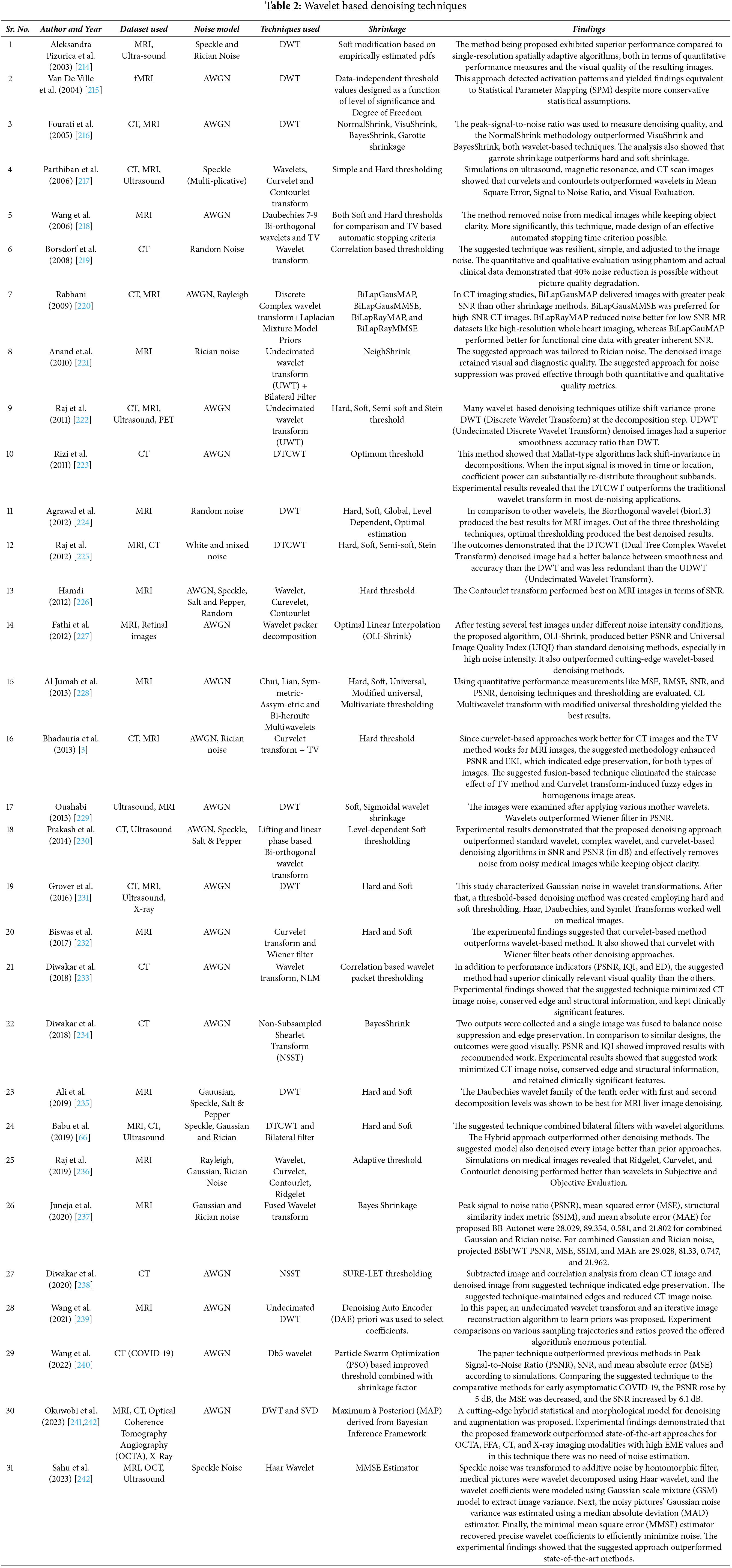
S. Mallat proposed an orthonormal filter bank based multi-scale/multi-resolution representation framework for images in [205,206]. Orthonormal low-pass and high-pass filter banks were used separate the images based on the frequency content present in the images, in that framework. These separated sub-bands are then subjected to thresholding operation to remove the noise present within. The factors that influence the performance of the Wavelet transform are the choice of mother wavelet, levels of decomposition and the type of thresholding applied. Availability of different types of mother wavelets viz. Daubechies (db), Haar (db2), Biorthogonal (bior), Reverse Biorthogonal (rbio), Symlet (sym), Coiflet (coif), Fejer-Korovkin (fk), etc. provide flexibility in terms of operation. A suitable “mother wavelet” can be chosen based on the requirement while choosing an optimum level of decomposition is also very important [204–208]. The wavelet transform evolved over time with introduction of Dual Tree Complex Wavelet Transform (DTCWT) [209], Curvelets [210], Contourlets [211] and Shearlets [212,213]. These transforms tried to achieve more directionality, shift invariance and better artifact mitigation capabilities. In the realm of signal processing, the Dual-Tree Complex Wavelet Transform (DTCWT) overcomes the challenge of shift-variance that plagues conventional wavelet transforms. Conversely, Curvelets, a specialized transform, exhibit remarkable prowess in effectively representing and analyzing curved features within images. Contourlets, conversely, were designed with the primary objective of capturing and representing continuous contours and boundaries within images, thereby rendering them highly advantageous for the execution of intricate operations such as image segmentation and object recognition [203]. Table 2 summarizes the various wavelet based denoising techniques.
In a parallel manner, Shearlets were devised to effectively address the anisotropic characteristics present in images, encompassing edges and textures, through the acquisition of their directional attributes across various scales. The recent progressions in wavelet transforms have significantly enhanced the precision and efficacy of algorithms used in signal and image processing. This has facilitated the ability to conduct more meticulous analysis and manipulation of intricate data. The main type of artifact arousing from X-lets is ringing artifact due to Gibbs phenomena. Ringing artifacts occur at sharp discontinuities in image due to finite approximations. Better noise reduction was also achieved by adopting optimum sets of parameters in Self-Organizing Migration Algorithm (SOMA). In SOMA, parameters like levels of decomposition, type of wavelet, and the type of thresholding were found for wavelet shrinkage denoising to achieve maximum performance [243]. This algorithm is fairly explored in [243–246].
The Wavelet transform successfully encodes the energy of the signal into fewer significant coefficients with remaining insignificant coefficients related to the signal independent noise. In threshold system for denoising, the threshold is required to separate the structural information from the noise. But practically it tends to over-smooth the signal. The efficiency of the denoising algorithm depends on the effective modelling of the inter-scale and intra-scale dependencies between the decomposition levels, presented by the Wavelet transform. Several techniques aimed at exploitation of these dependencies to improve their performance. Additionally, the imposition of down-sampling on Wavelet transform makes it translation variant [13]. As a result of this, visual artifacts in the form of Gibbs phenomena are introduced in the image. To address these issues, in [247], Linear Minimum Mean Square Error (LMMSE) was used for wavelet coefficients in place of soft thresholding. LMMSE scheme achieves efficiency by reducing the statistical estimation error through adaptive spatial classification of Wavelet coefficients. Despite being suitable for the denoising of many images, it proved to be unsuitable for weakly correlated images in the scale space.
Block Matching and 3D filtering method is a state-of-the-art image denoising technique proposed by Dabov et al. in [248]. BM3D is the one of the best techniques for denoising available till now. It is a transform domain technique based on enhanced sparse representation. Grouping of similar 2D image patches (blocks) to form 3D groups is done to achieve enhanced sparsity. After that, collaborative filtering is done on these 3D groups in three steps viz. transformation, shrinkage and inverse transformation. The collaborative filtering outputs revels the finest details shared by the groups, simultaneously preserving unique features present in each block [247]. In [249], BM3D and other state-of-the-art techniques were used and compared on MRI images. It was found that Unbiased Non-Local Means filter and BM3D hyrid with Spatially Adaptive Principal Component Analysis performed better than the other techniques. Pulse Coupled Neural Networks (PCNN) are 2-dimensional neural network, modelled using the cat’s visual cortex system. Its proposition goes back to 1989 when the concept of linking field was explained by Reinhard Eckhorn through which a correlation between attribute linking and perceivable functions could be set up [250,251]. Then after 1994, this neural model was adapted in image processing with name PCNN and till now it has found its application in various fields of image processing and computer vision like motion sensing, feature retrieval, segmentation, enhancement, restoration, fusion, region growth and denoising, etc. What makes this network attractive for computer vision application is its inspiration which comes from the operation of neurons in the primary visual field. So, in context of an image a pixel is represented by a neuron in PCNN. The color information is taken as an outside stimulus and the local stimuli is received from the surrounding neurons by setting up a connection. Then these stimuli are merged in an activation system and an output pulse is generated when the combination reaches a decided threshold. A time series of pulse outputs is generated by iteratively repeating this process. Then different functions are carried out using that time series [251,252].
A simplified version of PCNN known as spiking cortex model was also introduced in 2009. The threshold function for the PCNN is an evolution of neural analog threshold given as
where,
Here,
and
PCNN is a non-linear denoising method with a slow response and parameter dependence [251].
In Total Variation (TV) regularization, it is assumed that the signal with too much irrelevant details have high total variation. This means that absolute gradient’s integral is high. So, minimum total variation is aimed in case of image smoothing by simultaneously preserving relevant edges. A general TV-
where,
Total variation (TV) regularization based image denoising techniques are explored extensively for medical images. In 2006, a new denoising scheme based on TV minimization and wavelets was proposed for medical images [218]. Later in 2011, by examining the needs of medical image characteristics from the perspective of image denoising, a denoising algorithm based on partial differential of total variation was presented [129]. Subsequently, a new technique based on TV was proposed for medical images corrupted by Poisson noise. The study formulated the denoising issue using Bayesian statistics. This was done by establishing a nonnegativity-constrained minimization problem. This problem’s objective function had two terms: the Kullback-Leibler divergence for data fitting and the Total Variation function for regularization. The regularization parameter weighted the term. This paper aimed to propose a powerful computational method for tackling the constraint issue. The Newton projection method resolved the internal system using the Conjugate Gradient approach. This approach was preconditioned and optimized for the application [127].
Later on, many more techniques based on TV were proposed specifically for the denoising of medical images, e.g., [3,120,254,255]. In [120], simple TV regularization was used to denoise medical images whereas in [3] and [255] TV regularization is used along with Curvelet transform and Anscombe transform respectively to carry out the denoising process. These hybrid methods produced excellent result in effectively reducing the Poisson noise problem prevailing in medical images. In [254], Fractional order TV was used with alternating sequential filters to achieve fusion of noisy medical image modalities. Dang NH Thanh in presented an excellent review and a comprehensive analysis of several significant techniques for Poisson noise removal in medical images. These techniques included the modified TV model approach, the adaptive non-local total variation method, the adaptive TV method, the higher-order natural image prior model approach, the PURE-LET method, the Poisson reducing bilateral filter, and the variance stabilizing transform-based methods [7].
Markov properties are the properties, followed by a set of random variables called undirected graphical fields. These fields are also called Markov Random Fields (MRF) [256]. In terms of representation of dependencies, MRF is very similar to Bayesian network. The only difference that exists is that the Bayesian networks are acyclic and directed. A random variable forms an MRF if local Markov properties are satisfied. There are these properties named, Pairwise Markov property, Local Markov property, Global Markov property. In these properties, dependencies of the variables with respect to other variables are declared. The Global Markov property is strongest, followed by Local Markov Property, followed by Pairwise Markov property. Performing a full Maximum-A-Posteriori (MAP) for inference in MRF is very slow [257,258]. To address this problem a suboptimal inference algorithm called Active Random Field (ARF) was proposed by Adrian Barbu in [259]. It is a combination of Markov and Conditional Random Fields. The ARF provides a strong MAP optimum with lower number of iterations and it avoided overfitting by employing a validation sets to detect overfitting. Results showed that the one iteration Active Field of Experts (FOE) was as efficient as 3000 iteration FOE.
The prior modelling of an image is used in many computer vision applications. These prior models are used whenever there is noise and uncertainty in picture. The prior models are also known as depth maps or flow fields. For low level vision problems, methods are developed for learning priors. The priors are then computed for large neighbourhood systems, and for that sparse image patch representations are exploited. One of the important methods for sparse coding is Gaussian Mixture Models (GMM) [161,260] and Generalized Gaussian Mixture Models (GGMM) [261]. The models of prior probability are called Fields of Experts (FoE) [262]. In other words, Fields of Experts are used to model natural images for which the standard database of natural images is trained. Due to large dimensions of images and their non-gaussian statistics, modelling of the image priors is a difficult task. A number of attempts have been made to overcome these difficulties and to model the statistics of small image patches as well as of entire images. So, the major goal in this field is to develop a framework for learning generic and expressive prior models for low level vision problems.
Generally, the Field-of-Experts model is defined as
where,
The FoE model share some similarities with Convolutional Neural Networks (CNNs) where, filters banks are applied in a convolutional manner, to the whole image and the filter responses are modelled by using a non-linear function. The only significant difference lies in the training of both models. The convolution networks are trained for specific applications in a discriminative fashion while, the FoE models are trained in a generic manner by learning a generic prior which can be used in different applications. This is because of the probabilistic nature of FoEs [262].
The traditional patch prior based systems for image denoising were computationally complex due to large search windows used to evaluate pairwise similarity. The evaluation of the similarity is needed to generate correlation between the pixels of the target image. As, in natural images, redundancy is primarily presented at a semi-local level. Based on this observation, the patches (local neighbourhood sets) which are used to represent the images are made to collaborate. This collaboration is independent of the spatial position of the pixels. On the prior assumption that the noise infecting the image is additive in nature, the denoising process aims at estimating the an image out of its noisy version. So, a simplified model of the noise is required to effectively denoise the image. To obtain a simplified noise model approximated by a white Gaussian noise, stabilization of the noise variance is done with the help of Anscombe transform. The generalized degradation model for an image is written as
where,
Apart from Gaussian Mixture Model (GMM), Laplacian Mixture Models (LMM) are also used in the image denoising paradigm. The Gaussian Mixture Model (GMM) is an appropriate choice for datasets that exhibit clusters resembling the Gaussian distribution. On the other hand, the Laplacian Mixture Model (LMM) demonstrates greater resilience to outliers and data that deviates from the Gaussian distribution. The Gaussian Mixture Model (GMM) may encounter challenges when dealing with heavy-tailed data and outliers due to the inherent nature of the Gaussian distribution, which is characterized by light tails. The LMM may exhibit an inclination to overestimate the quantity of clusters when confronted with noise, owing to the heightened susceptibility of the heavy tails of the Laplace distribution to the presence of noise. The Gaussian Mixture Model (GMM) exhibits heightened sensitivity towards the covariance structure of the data, whereas the Laplacian Mixture Model (LMM) places comparatively diminished emphasis on the estimation of the covariance matrix owing to the presence of exponential tails. In essence, the selection between Gaussian Mixture Models (GMM) and Laplacian Mixture Model (LMM) is contingent upon the inherent attributes and properties of the data that is being subjected to modelling. In [220], Bivariate LMM was used to denoise medical images.
GGMM prior is more flexible and it can model natural images better than GMM prior and Expected Patch Log-Likelihood (EPLL) framework is used often for optimization [263]. EPLL is a classical external patch prior based framework and it is more efficient when compared to internal patch priors, in case of images with higher noise levels [154]. Some other examples of external patch priors based methods include Gradient Histogram Preservation (GHP) [264–266].
Fig. 6 illustrates the patch-prior-based denoising process. It is known that for natural images particularly, Gaussian potential is not suitable. Therefore, filters that fire rarely on natural images are sought out. To identify such filters, a well-known and consistent observation is followed. According to this observation, the power spectrum of natural images tends to decrease with increasing spatial frequency. So, filters with power concentrated in high spatial frequencies are considered for maximum likelihood. The perfect example of such filters is Roth and Black filters, which are frequently used in the case of GSM priors. However, these filters exhibit some drawbacks in lower and upper bounds on the maximum likelihood of the training set. These drawbacks are addressed by considering the possible rotations of basis set (BRFOE) of the filter. To carry out this operation, a basis rotation algorithm is applied to the set of the filters, having power spectrum same as the Roth and Black filters. This results in filters with more structure and extended bounds [267].

Figure 6: Patch-prior based denoising
In comparison to several parametric methods discussed earlier, the nonparametric methods rely on the data to decide the structure of the model. This implicit model is called as regression function and this idea of nonparametric estimation is called as kernel regression. Several concepts related to the general theory of kernel regression has been presented earlier for, e.g., edge-directed interpolation, bilateral filter, moving least squares and normalized convolution. The study of their relation with the general kernel regression theory has been done in [268] and an adapted non-linear kernel regression framework was proposed. In general, this method of filtering is very similar to local linear filtering process and suffers poor reconstruction on edge areas because of its non-adaptiveness near the edges.
Despite the efficacy of the orthonormal bases in sparsely representing the signal, they are inadequate for some specific signals of interest. Instead of orthonormal bases, sparse-based denoising techniques require a trained dictionary to sparsely represent a signal. So, by using an algorithm for sparse approximation a signal

In [279], GSR was used with dictionary learning for the denoising and fusion of CT and MRI images. Sparse coding-based methods has also been explored extensively for multi-modal medical images for, e.g., in [281], a novel global approach based on sparse representation and NLM was adopted to denoise multi-modal medical images. This method effectively denoises images while preserving sensitive tissue details. A sparse coding-based dictionary learning method has also been employed to denoise 3-D medical images [282]. On the same note, a deep learning based framework (unsupervised) was proposed for the denoising of 2-D as well as 3-D medical images [157]. Later on, a combination of medical image denoising and fusion was achieved by hybrid variation sparse representation based on a decomposition model [283] and sparse dictionary learning via discriminative low rank [284].
The fundamental objective of the Weighted Nuclear Norm Minimization (WNNM) technique is to effectively utilize the inherent properties of low-rank and sparse structures that are inherently present within matrices of data. This formulation entails the optimization of a convex objective function that comprises two fundamental components. The first component is the nuclear norm of a matrix with low rank, which quantifies the overall magnitude of the singular values of the matrix. The second component is the weighted ℓ1-norm of a matrix that is sparse, indicating that it contains a significant number of zero or near-zero elements. The utilization of the nuclear norm facilitates the achievement of low-rank approximation by effectively capturing the latent structures that are intricately embedded within the data that is subject to noise. Conversely, the weighted ℓ1-norm is employed to impose sparsity, thereby enabling the representation of noise or outliers in a concise manner [285,286].
The optimization problem linked to Weighted Nuclear Norm Minimization (WNNM) is characterized by its intricate complexity, primarily due to its combinatorial properties and non-convex nature, which stem from the inclusion of the nuclear norm. As a result, the utilization of efficient proximal algorithms, coupled with the incorporation of proximal gradient techniques, is employed to approximate the solution. The aforementioned iterative methodologies employ iterative processes to iteratively modify the low-rank and sparse components, taking into account the weighted regularization factors [287]. In order to guarantee the convergence of a computational algorithm, it is common practice to incorporate adaptive step size selection methodologies and convergence acceleration techniques, such as the renowned Nesterov’s acceleration method [288–290].
The effectiveness of Weighted Nuclear Norm Minimization (WNNM) relies on the prudent choice of the regularization weights, which have a crucial function in achieving a harmonious equilibrium between the low-rank and sparse elements. The weights in question encapsulate a pre-existing understanding of the data and its noise properties, allowing for customization to suit particular applications. The selection of weights that are optimal in nature results in representations that have been denoised or compressed, thereby effectively retaining crucial features while removing any noise or extraneous data components [286].
The fundamental foundation of WNNM resides in its capacity to exploit the concurrent utilization of low-rank approximation and sparse representation. The confluence of these factors results in heightened denoising efficacy, versatility in accommodating diverse noise distributions, and resilience in the face of fluctuating noise intensities. Moreover, the Weighted Nuclear Norm Minimization (WNNM) algorithm can be expanded to incorporate situations that involve the processing of multichannel data, temporal correlations, and heterogeneous noise structures [285]. In [291], the concept of nuclear-norm minimization was used with Rolling guidance filter and CNN to achieve effective multi-modal medical image denoising. In [292], also, WNNM was used to denoise 3-D medical images. Given the inherent complexity of the original problem pertaining to low-rank approximation, the prevailing approach commonly employed involved the utilization of nuclear norm minimization as a means to achieve matrix low-rank approximation. Notwithstanding, the solution derived through the process of nuclear norm minimization typically exhibits a deviation from the solution of the initial problem. A proposition is put forth for the denoising of MR images through the combination of a nonlocal self-similarity scheme with a pioneering low-rank approximation scheme [293].
Adaptive Clustering is a sophisticated computational methodology that effectively tackles the intricacies of unsupervised clustering by employing a dynamic approach to modify cluster attributes in accordance with the specific characteristics of local data. Conventional clustering algorithms frequently encounter difficulties when confronted with data points that manifest diverse densities, shapes, or sizes. The technique known as Adaptive Clustering effectively mitigates the aforementioned limitations by employing a dynamic estimation process to determine the most optimal number of clusters. Additionally, it adapts the parameters of each cluster to more accurately capture the nuanced distribution of the data [294,295].
Progressive PCA Thresholding iteratively captures and retains the most useful features in high-dimensional data, solving its problems. Traditional Principal Component Analysis (PCA) reduces dimensionality, but tiny eigenvalues, due to their cumulative effect, can cause information loss in high-dimensional data. A staged eigenvalue thresholding procedure defines Progressive PCA Thresholding. Eigenvalues are ordered in decreasing order of importance and kept above a dynamically defined threshold in each stage. This progressive technique considers just the most impactful eigenvalues and their eigenvectors, resulting in a parsimonious data representation that keeps its intrinsic variance. Progressive PCA Thresholding also uses adaptive regularization to account for data structure differences across dimensions. The approach finds dimensions with low variance and suppresses their contributions to the main components using data-driven sparsity constraints, improving the reduced representation. Progressive PCA Thresholding shines in genomics and hyperspectral imaging, where data dimensionality surpasses sample quantity. Eigenvalue thresholding and sparsity-driven regularization enable adaptive feature extraction while reducing noise and small fluctuations [295].
Similarly, ACVA works on the idea that images have local structures or patches with different noise and image properties. The approach starts with adaptive clustering of related patches. This clustering algorithm groups patches with similar features based on noise levels and structural patterns. After adaptive clustering, ACVA uses variation-adaptive filtering in each cluster. This filter uses local variation data to dynamically alter its settings. ACVA reduces noise while keeping vital characteristics by responding to image patch texture and content fluctuations [296]. Also, Adaptive Soft-Thresholding (AST) Based on Non-Local Samples (NLS) is e technique where adaptive signal modelling is used with adaptive soft thresholding to achieve effective denoising performance [297].
3.4 Deep Learning Based Denoising
In the current scenario, Convolution Neural Networks (CNNs) and Machine learning based image denoising techniques are being rapidly explored and used in medical image denoising [298]. The Denoising Convolutional Neural Network (DnCNN) is an advanced computational framework specifically engineered for the purpose of image denoising. The proposed system utilized a multi-layered convolutional neural network architecture to acquire knowledge of the complex relationship between input images contaminated with noise and their corresponding clean, denoised counterparts. The DnCNN model has been meticulously designed to efficiently eliminate noise from images by capitalizing on its innate capacity to acquire knowledge and depict intricate noise patterns and image structures via the network’s hierarchical feature extraction procedure.
The fundamental principle underlying DnCNN involves the utilization of a residual learning framework, wherein the neural network is trained to accurately forecast the residual noise element that exists between the input signal contaminated with noise and the intended clean output signal. The utilization of a residual-based methodology enables the neural network to effectively concentrate its attention on the specific noise components that require elimination, rendering it highly suitable for the task of image denoising. The architecture of DnCNN is comprised of a multitude of convolutional layers, typically arranged in a cascaded fashion. The aforementioned layers systematically and incrementally extract and enhance visual attributes of an image, all the while inherently encapsulating the inherent characteristics of noise. The utilization of batch normalization layers is a common practice in order to achieve stabilization and acceleration of the training process [299].
In the context of medical image denoising, in [300], a proposition for a strategy known as content-noise complementary learning (CNCL) was proposed. This strategy, while straightforward in nature, has proven to be highly efficient. It involved the utilization of two deep learning predictors, each tasked with learning the content and noise of the image dataset in a complementary manner. A novel medical image denoising pipeline was introduced, employing the Convolutional Neural Network with Cascaded Non-Local (CNCL) strategy. The pipeline is realized as a Generative Adversarial Network (GAN), with an exploration of multiple representative networks such as U-Net, DnCNN, and SRDenseNet as the predictors. Similarly, in [301], methodology involved the utilization of residual learning as a prominent learning approach, coupled with the incorporation of batch normalization as a means of regularization within the deep model [301], and in [302], a Genetic Algorithm (GA)-based methodology was introduced to facilitate the exploration of optimal genetic traits for the purpose of optimizing network structures.
In addition to general-purpose models, several advanced deep learning architectures specifically for medical image denoising have been made available in recent years. Since U-Net and its extensions (like Attention U-Net and U-Net++) are capable of learning both local and global context, they are especially popular due to their ability to maintain subtle anatomical details in noisy medical images. In the same vein, by enhancing hierarchical feature extraction and encouraging gradient flow in deep layers, Residual Dense Networks (RDNs) and SRDenseNet have been adapted for denoising purposes. Low-dose CT and MRI reconstruction is now employing architectures such as DRUNet, which was developed for blind denoising, and FFDNet, which is for adaptive denoising under varying noise levels. Table 4 summarizes the various deep learning based image denoising techniques.
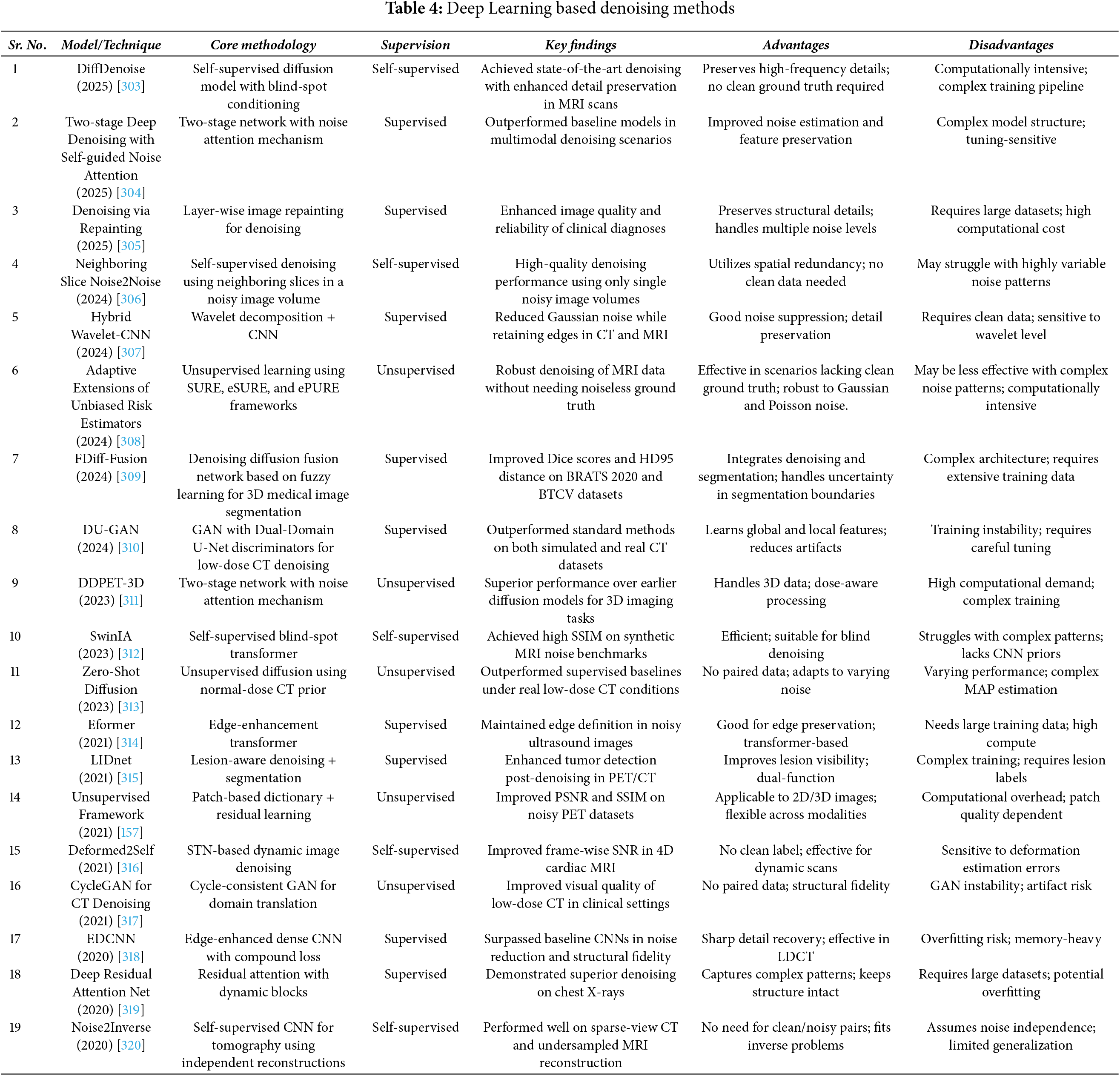
Additionally, through data-driven prior learning, GAN-based models (e.g., Noise2Noise GAN and Pix2Pix for MRI Denoising) have shown promising results in producing outputs that are perceptually improved.
3.5 Hybrid Deep Learning for MRI/CT Image Denoising (2019–2024)
Noise, such as thermal noise in MRI and quantum noise in low-dose CT, can frequently disrupt medical imaging and obscure critical information. Spatial filters (such as Gaussian smoothing, bilateral filters, Non-Local Means, BM3D, and anisotropic diffusion) and frequency-domain transforms (including wavelet and Fourier filtering) exemplify conventional denoising techniques that perform adequately but fail to effectively capture intricate details. In recent years, deep learning (DL) has emerged as a formidable alternative, effectively learning to transform noisy images into clean ones with remarkable efficacy [321,322]. Metrics such as PSNR and SSIM indicate that pure deep learning approaches, such as CNN denoisers, generally outperform classical filters [322]. However, they may encounter issues like as excessive smoothing, artifacts, or inadequate generalization to novel noise distributions [321,323]. This has resulted in hybrid approaches that combine conventional denoising filters or transformations with deep neural networks to optimize outcomes. These hybrids leverage domain expertise, such as edge preservation, frequency sparsity, and self-similarity, to enhance the performance and stability of data-driven models.
Recent study indicates the existence of numerous varieties of these hybrid techniques. A 2024 assessment of 104 papers revealed that CNN-based models were the most prevalent, comprising approximately 40%, followed by encoder-decoder networks at around 18%, Transformers at about 13%, GANs at approximately 12%, and others thereafter. This illustrates the variety of deep learning architectures that have been examined. The types of noise discussed encompass Gaussian (about 35% of articles), speckle (16%), Poisson (14%), Rician (7%), and more variants. We shall now examine some significant hybrid approaches categorized into two primary groups: Deep Learning utilizing Spatial Filters and Deep Learning employing Frequency-Domain techniques. We discuss the methodologies and architectures employed, the datasets and evaluation metrics applied, the application domains (such as low-dose CT and rapid MRI), the comparative efficacy of each approach, as well as the advantages, disadvantages, and emerging trends associated with each method.
3.5.1 Deep Learning Meets Spatial Filters
This group of hybrid approaches combines standard spatial-domain denoising filters with a deep learning framework. The goal is often to add inductive biases to neural networks, like edge-awareness or self-similarity, or to employ a classic filter as a way to improve the output of a network. Some important instances are:
a) Non-Local Means and Deep NetworksNon-Local Means (NLM) uses redundancy by averaging similar patches throughout the whole image. Deep models have taken this principle of self-similarity and used it. For instance, CNLNet (2025) includes an NLM filtering layer in a CNN design for brain MRI denoising [324]. The network does this by combining learnt feature extraction with the NLM’s capacity to use repeated structures. This makes it better at keeping details than a CNN alone. In fact, when you put CNLNet (with NLM) and an equal CNN without NLM next to each other, you could see that CNLNet made brain MR images that were cleaner and more accurate in terms of structure. Liu et al. (2022) also suggested a “dense hybrid convolutional network” that combines a deep CNN with a typical non-local filter in a blind denoising environment [325]. Putting non-local activities or attention processes inside networks is becoming more common. This was based on the success of non-local neural networks in computer vision, which showed that modeling long-range pixel interactions can greatly improve denoising performance [324]. Attention-based denoisers that use modern transformers naturally capture global self-similarity, which is similar to NLM. This makes it harder to tell the difference between learnt and non-local filtering methods. Overall, adding NLM principles to DL has helped reduce noise without making small details less clear, but it has made the network more complicated.
b) BM3D and CNN HybridsBM3D (Block-Matching and 3D filtering) is a standard denoising technique that puts similar 2D patches into 3D stacks and uses collaborative filtering, like hard-thresholding in the transform domain. BM3D works well for moderate noise, while pure CNNs currently commonly have higher PSNR. There have been attempts to merge them via hybrid methods. One way to do this is to use a two-stage cascade, where first a CNN denoiser is used and then BM3D, or the other way around. For example, Krylov’s 2019 technique showed a hybrid DnCNN + BM3D pipeline with an automatic way to choose BM3D’s strength parameter [326]. The goal of this strategy was to allow the CNN get rid of most of the noise while the BM3D took care of the remaining structured noise, keeping the anatomical features intact. According to Krylov, the hybrid did better than either DnCNN or BM3D alone in PSNR at different degrees of noise. When ground truth is not available, another way is to utilize BM3D as a teacher to train a network. For example, researchers have utilized BM3D-denoised images as stand-ins for real noisy scans to train deep models, taking use of BM3D’s known reliability. One study, on the other hand, discovered that a network trained on BM3D outputs did a little worse than one trained on real clean images. This suggests that BM3D can assist start a network, but it can eventually do better than BM3D with the right supervision. Iterative reconstruction methods sometimes use BM3D as a regularizer in low-dose CT. Recently, learning-based variants of these plug-and-play systems have come out. In general, BM3D+DL hybrids can help keep structures intact and make denoisers work better, although they do add extra processing steps. They also have the same problems as BM3D (fixed transform thresholding), which could limit their eventual performance if the CNN’s full potential is not used [327].
c) Bilateral and Guided Filtering with Deep LearningBilateral filters (BF) smooth out edges by averaging pixels with similar intensity (range filter) in a spatial vicinity. They are useful because they keep edges while getting rid of light noise. Wagner et al. (2022) came up with a strong hybrid method for low-dose CT that puts trainable Joint Bilateral Filters (JBF) into a deep pipeline [323]. A CNN first predicts a guidance image (an initial denoised version), and then a collection of trained bilateral filter layers uses that guidance to clean up the noisy input. This hybrid worked much better on CT scans with noise and artifacts that were not in the training set because it combined the high capacity of CNNs with the known dependability of bilateral filtering. For instance, when the hybrid JBF method was tested on CT slices with metal artifacts (which were not visible during training), it raised PSNR by a few percent and RMSE by 6–10% compared to utilizing the CNN alone. The trainable BFs operate as a safety net, making sure that the network does not make outputs that are quite abnormal. Another study (Maier et al. 2019) showed that adding known linear filter operations to neural networks can definitely lower the limits on errors [328]. In reality, a shallow CNN taught to operate like a bilateral filter (BFnet) can do better than a hand-made filter by learning the best kernels while still being easy to understand. Guided filters (also called edge-aware filters) have been used as post-processing for DL denoisers to make edges even sharper. In the non-subsampled shearlet domain, a 2024 study paired a CNN with an edge-guided filter. This gave CT images a PSNR that was 3–4 dB greater than using wavelet denoising alone [329]. In general, bilateral filter hybrids improve edge retention and stability, making the denoising more resistant to varied amounts of noise and stopping the “blurring” that a pure CNN might cause around delicate structures.
d) Anisotropic Diffusion and Deep Prior FusionAnisotropic diffusion (AD) is a type of filtering that smooths an image while stopping diffusion across borders. It is based on the Perona–Malik filter. This is a well-known way to get rid of noise and keep edges. Researchers have recently been looking into how to combine these types of diffusion models with deep learning. One way to learn or manipulate the diffusion coefficients is to utilize a CNN. For example, deep image prior with non-local regularization added a non-local diffusion prior to the loss function of an untrained network, which made denoising better without any help [326]. Another example is MPDenoiseNet (2025), which is a multi-path network that has Anisotropic Diffusion blocks and convolutional layers [330]. There are two paths in MPDenoiseNet that process the image. One path has regular CNN layers that target various types of noise, while the other path has a differentiable anisotropic diffusion module that smooths the image without losing the edges. The outputs are then combined (in their case, with Transformer-based attention) and sent to a U-Net for final reconstruction [330]. This design successfully combines model-based and learning-based methods. The diffusion blocks keep the structure intact, and the CNN/Transformer parts get rid of complicated noise. According to reports, MPDenoiseNet was able to denoise images as well as the best ones, such the Restormer transformer, while utilizing a lot fewer parameters. This was possible because of these efficient diffusion-inspired modules [330]. Adding AD helps with stability since it directly models the smoothing process, which cuts down on streak artifacts and over-smoothing. One problem is that it can be hard to tune the diffusion settings, even if you know how to do it. These hybrids may also need to carefully balance the learnt and fixed operations to avoid artifacts like the staircase effect from diffusion or noise that is still there because of not learning enough. Deep/diffusion hybrids, on the other hand, show a potential path by adding interpretability and physical reasoning to neural networks for denoising.
3.5.2 Deep Learning Meets Frequency-Domain Techniques
Another class of hybrid denoisers operates (partly or wholly) in the frequency domain. These methods leverage transforms like wavelets, Fourier, discrete cosine transform (DCT), or more specialized multiscale transforms (Shearlets) in conjunction with deep networks. The rationale is that many medical images have sparse representations in certain transform domains (e.g., wavelet coefficients) and that filtering in those domains can be very effective at separating noise from signal. Hybrid approaches can integrate transforms as a pre-processing step, post-processing step, or even embed the transform within a network architecture.
a) Wavelet-Enhanced Deep Networks
Wavelet transforms break images down into sub-bands with different resolutions, such as low-frequency approximations and high-frequency details. In these sub-bands, noise can often be found and set to a certain level. There have been a number of studies that have used wavelet methods and CNNs together to clean up medical images. The MWDCNN (Multi-Stage Wavelet Denoising CNN) by Tian et al. (2023) [331] is a good example. This network has wavelet transform blocks built into it. After an initial conv layer, it does two stages of wavelet decomposition and augmentation (denoising) before using an inverse wavelet transform and more CNN refinement to put the image back together [331]. The network learns to filter wavelet coefficients using layers that may be trained, which reduces noise in each sub-band. MWDCNN may recover fine details better than solely spatial CNNs because it uses both signal processing (hard/soft thresholding effect in wavelet domain) and discriminative learning. It did better than well-known denoisers, like regular CNNs, in both quantitative and visual quality.
Zangana and Mustafa (2024) did another study that was simpler. They first used a wavelet transform on the noisy image, then used a CNN to remove noise from the approximation coefficients (the low-frequency part) while either throwing away or thresholding the detail coefficients. Finally, they put the image back together. This hybrid reduced noise much more than just wavelet thresholding, and it did not lose any image information [307]. The CNN’s concentration on the coarse structure (where most energy is) and the wavelet’s ability to separate out high-frequency noise are what make it useful. In the same way, DST-Net (2021) added a Discrete Shearlet Transform (a directed multiscale transform similar to wavelets) to a CNN, which made it better at removing noise from images with fine textures [324]. That gave rise to recent work in 2024 that merged CNNs with Non-subsampled Shearlet Transforms (NSST) to clean up CT scans. For example, a method-noise CNN (which learns to remove only noise residual) was used in the shearlet domain and paired with Bayesian thresholding of shearlet coefficients [332]. This hybrid had the best PSNR/SSIM across a range of noise levels when compared to techniques that only used spatial or transform methods.
The wavelet/shearlet-based hybrids tend to fare better at keeping the structure of the image intact—edges and textures are better preserved—and they often work well across different levels of noise because thresholding in a transform domain does not care much about noise variation (up to a point). One drawback of using fixed transforms is that they could make the network less flexible (the network has to function within the limits of the transform), and the transform operations use more processing power. Still, because medical image characteristics are generally multi-scale, wavelet-integrated deep denoisers have been highly useful, especially for low-dose CT scans where keeping edges (such bone borders) is very important.
b) Fourier/DCT Domain Approaches
Sometimes the Fourier domain (k-space for MRI) or DCT is used for hybrid approaches. It is customary to work in k-space while reconstructing MRI images. Some researchers have tried filtering noise in frequency space using learning models to get rid of noise in fully sampled MRI images. For instance, a network might take an image’s FFT, use a deep filter to get rid of high-frequency noise, and then invert it back. These kinds of methods can naturally get rid of noise that is not correlated in space, which shows up as broad-spectrum components. One problem is that the noise in the MRI images (magnitude images) is Rician, which does not turn into a simple distribution in k-space after reconstruction. So, most DL MRI denoisers still work in the image domain. But in CT, there are hybrid dual-domain networks that can denoise both image data and projection data (Fourier/Radon domain). DuDoNet (2019) [333] is one example. It had two branches: one worked with sinogram data and the other with reconstructed images. It used cross-domain regularization to combine Fourier-space processing with image-space CNN. Compared to single-domain networks, these dual-domain methods did a better job of getting rid of noise and artifacts in low-dose CT scans. They take advantage of the fact that some noise or artifacts might be easier to fix before back projection (in CT) or before inverse FFT (in MRI).
Another intriguing change is that people are now seeing conventional DCT filtering as a neural network. DCT2Net (Herbreteau & Kervrann 2022) showed that a typical DCT-based denoiser (which applies a blockwise DCT, thresholds coefficients, and transforms back) can be made into a shallow CNN and adjusted using learning. They built a network that can be understood using DCT kernels and even suggested a mix of the learnt DCT2Net and the original DCT approach. The network takes care of textured patches that are hard to understand, while the classical DCT filter takes care of smooth areas [334]. This gave results that were around the same quality as BM3D but with a lot fewer layers. It also helped me grasp how frequency filters work with CNNs. DCT2Net was shown on natural photos, but the approach can also be used in medical imaging to make denoising solutions that are easy to see.
In short, frequency-domain hybrid methods add multi-resolution and frequency-selective filtering to deep learning. They are especially useful for things like low-dose CT (where noise has a strong high-frequency component and transform-domain denoising can get rid of noise before reconstruction) and rapid MRI (where undersampling artifacts/noise can be dealt with in k-space). The biggest problem is that working in the transform domain can make network design more difficult, especially when working with MRI data that is hard to understand. If the two domains are not carefully balanced, mistakes in one domain might cause artifacts in the other. However, so far, the results demonstrate that these hybrids typically do better than solely spatial CNNs on objective criteria and keep the quality of diagnostic images better (clearer edges, less oversmoothing).
3.5.3 Datasets and Evaluation Metrics
Researchers have evaluated these denoising methods on a variety of datasets, using standard image quality metrics:
• Datasets (CT): The Mayo Clinic Low-Dose CT dataset (from the 2016 AAPM Challenge) is a typical standard for low-dose CT denoising. It has pairs of clinical CT scans with normal doses (NDCT) and quarter doses (LDCT). This dataset is used to train a lot of deep learning models, like GANs and CNNs [325]. Some people use the LoDoPaB dataset (a big public low-dose CT set) or fake phantoms. Some studies employ private clinical CT scans (such abdomen or head CTs) with extra noise added to make it look like a lower dose. For example, Wagner et al. (2022) trained on belly CTs and then tested on a separate set of CTs with metal inserts and head CTs to see if the model could generalize.
• Datasets (MRI): It is tougher to get ground-truth MR images that do not have noise. So, a lot of MRI denoising publications use simulated noise. The BrainWeb MRI phantom and the McGill dataset are two resources that are often used. They provide fake MRI scans with known noise levels (Gaussian or Rician). Some studies use many scans of the same person (for example, averaging multiple acquisitions for ground truth). The NYU fastMRI dataset, which was originally created for faster MRI, has been changed by adding fake noise to fully-sampled data. Researchers typically employ brain MRI datasets (T1-weighted brain scans from IXI or the Human Connectome Project) with added noise to test denoisers [324]. There have also been MICCAI challenges that focus on removing noise from MR images, such the MRI denoising challenge at MICCAI 2013, which used genuine noisy scans and fake ground truth. Overall, brain MRI is the most prevalent type of denoising study. However, some research use HCP data to look at diffusion MRI (DWI) denoising, and others look at cardiac or abdominal MRI with added noise.
• Metrics: Peak Signal-to-Noise Ratio (PSNR) and Structural Similarity Index (SSIM) are the two main quantitative measurements. Almost all of the papers use these to compare the quality of denoising. PSNR is a logarithmic measure of the pixel-wise MSE, and SSIM measures how good an image looks by comparing its local structure, contrast, and brightness. Many studies also talk about Root Mean Square Error (RMSE), which is directly connected to PSNR, and sometimes Mean Absolute Error (MAE). Some research employ more complex metrics, like Feature SIMilarity (FSIM) and Entropy Difference (ED), to measure how well texture is preserved [329]. In clinical settings, task-specific metrics can show up, including how denoising affects diagnostic tasks (like how well lesions can be seen or how accurate segmentation is) or radiologist opinion scores. Some low-dose CT investigations look at how accurate the CT numbers are (Hounsfield unit errors) and how many streak artifacts there are. When looking at these measures, denoising methods are usually compared to classical baselines like the Gaussian filter, NLM, and BM3D, as well as alternative DL approaches like DnCNN, GAN models like DAGAN, transformer models, and so on. In general, hybrid approaches have greater PSNR/SSIM than their classical counterparts (sometimes by several dB PSNR) and are typically as good as or better than pure deep models. For instance, a Shearlet-CNN hybrid got about 3–4 dB more PSNR than regular wavelet denoising at all noise levels. On a given CT dataset, a bilateral-CNN hybrid from another work raised PSNR from about 40.0 to about 41.5 and SSIM from 0.90 to 0.93 compared to a baseline CNN. These numbers show that hybrid methods can improve image quality in a measurable way.
It is important to remember that PSNR and SSIM may not reveal the full story. For example, some approaches, like GANs, put more weight on visual realism than PSNR, whereas a pure MSE-trained CNN may produce high PSNR but lose little details. So, qualitative evaluation and clinical validation are still very important. Many studies provide radiologist ratings or sample images to show that diagnostic information is still there or has been improved.
3.5.4 Performance Comparison and Discussion
The landscape of denoising approaches now spans from pure classical methods to pure deep learning, with hybrids in between. Table 5 provides a high-level comparison of representative methods:
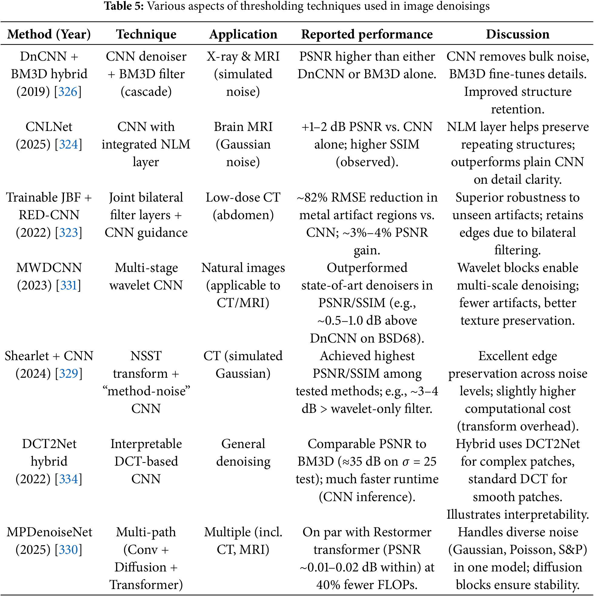
A few trends start to show up when you look at these comparisons. First, hybrid approaches typically work just as well or better than pure deep models when it comes to denoising, especially when there is not a lot of training data or when generalization is really important. For example, adding trainable bilateral filters to a CNN made it far more robust on CT data with structures that were not observed during training (like metal implants) [323]. This shows how classical filters may protect against new changes by enforcing recognized image priors, such as smoothness with edge preservation.
Second, hybrids are better at keeping anatomical details. A lot of pure DL models, especially those that optimize MSE, can make outputs that are too smooth. These outputs may have high PSNR but may also blur fine edges or textures that are critical for diagnosis. On the other hand, approaches like NLM-CNN or wavelet-CNN intentionally limit the solution to keep fine structures by using non-local averaging or thresholding in the detail sub-bands. Because of this, some approaches show higher SSIM and outcomes that are often clearly sharper. For instance, the CNLNet’s brain MRI outputs displayed tiny vessels more clearly than a regular CNN denoiser, thanks to the non-local filtering part.
Third, hybrid methods can help get around some of the problems with deep learning. The worries are about overfitting and not being able to generalize. For example, a network might work well with one scanner’s noise level but not with another’s. Classical approaches are usually not affected by the exact training data, even though they are not as powerful. When used together, technologies like Wagner et al.’s JBF pipeline made the network less likely to give outputs that did not make sense when it was faced with strange noise. This brought the outcome closer to a physically reasonable solution [323]. In the same way, hybrid models often need smaller networks or datasets: Using the DCT basis, DCT2Net got BM3D-level performance with a 2-layer network. This efficiency is useful in medicine, where there may not be a lot of training data or computing power available.
But there are some downsides to hybrid techniques as well. Adding classical parts can make the design more complicated and add more hyperparameters. In addition to all the network hyperparameters, a wavelet-CNN must also choose the type of wavelet, the number of levels, the thresholding approach, and so on. It can be hard to get the best results by tuning these. Some hybrids may also take on the failure modes of the classical element. For example, an anisotropic diffusion module could make “staircase” artifacts or get rid of little texture that a purely learnt model might have kept. Also, the extra processing (transforms or iterations) can make the algorithm run longer. Many CNN denoisers work in real time on recent GPUs, but a hybrid that uses iterative diffusion or needs many transform steps can be slower (albeit still quicker than iterative model-based approaches like total-variation minimization). In practice, studies say that the extra work is tolerable. For example, MWDCNN’s multi-stage technique is still rather quick, while DCT2Net is as fast as a tiny CNN. But these technologies need careful engineering to stay useful in the clinic.
3.5.5 Advantages and Limitations of Key approaches
To summarize the pros and cons of each hybrid strategy:
a) CNN + Spatial Filter (post-processing): (e.g., CNN → BM3D or CNN → bilateral filter)Advantages: Simple to use; takes advantage of CNN’s ability to remove noise and the filter’s ability to keep edges. Can greatly cut down on artifacts (the filter “cleans up” the CNN output). Helps in generalization (the filter smooths out noise that has not been observed before).Limitations: It is a two-step procedure, so you cannot train it all the way through, but the user may change the settings on validation data. Could smooth out some of the specifics that the CNN brought back (if the filter is too aggressive). Needs careful adjustment of the parameters, like the BM3D threshold or the bilateral sigmas. A little more time to make an inference because of the extra step.
• CNN with Integrated Filter Layer: (e.g., NLM or bilateral as a layer in the network)
Advantages: Full training means that the network may learn how much filtering to use in different situations. Keeps details because of the built-in previous (not local or edge-aware). Can be understood (you can look at the filter weights). Often gives better detail (higher SSIM) for the same PSNR.
• Limitations: Makes the network more complicated (non-local activities might use a lot of memory, and bilateral filtering in a net need to be set up in a certain way). Could make training take longer. If the integrated filter is not set up right, it could not be needed (the network could learn to get around it). Needs a lot of training data to set the filter parameters just right.
• Deep + Transform-Domain: (wavelet/shearlet + CNN)
Advantages: Multi-resolution analysis makes denoising better at all scales. It gets rid of fine noise in high-frequency bands and smooths out large-scale changes in low-frequency bands. Often great at not over-smoothing, which gives it outstanding visual quality (sharp edges). Can be more resistant to variations in noise level (thresholding schemes work with different σ).
• Limitations: Transform adds computations. The method might be changed to fit some noise statistics (for example, wavelet thresholding assumes that the noise is mostly additive Gaussian). If the noise has a structure that is not well captured in the transform domain (such MRI Rician noise or streak artifacts), the transform alone may not be enough and the network will need to make up for it. Also, if you design a neural network around a fixed transform, it might not be able to learn a different representation that is even better.
• Deep + Model-Based Iterative (Diffusion/PDE or Optimization):
Advantages: Includes strong physical priors (such edge continuity and noise smoothness) that can make denoising much more stable and reliable. Usually needs less training data and can sometimes work without supervision (for example, deep image prior with a regularizer). Can give estimates of uncertainty (with plug-and-play methods, the classical part can be understood).
Limitations: It can be slow because it goes through steps again and over. It is hard to find the right balance between data fidelity and prior (or between learnt component and classical component). If you rely too much on previous, the network might not denoise enough, and if you rely too little, it might hallucinate. When using diffusion + CNN hybrids, you have to make sure that the diffusion process does not smooth out important pathology too much (for example, tiny lesions can be viewed as noise). These methods are also harder to put into practice and think about in theory.
In real life, the method you use may depend on the area of application. For example, in low-dose CT, keeping edges and HU accuracy is very important. In this case, a wavelet or bilateral hybrid that is good at keeping edges could be the best choice. A review from 2024 found that encoder-decoder CNNs with MSE loss do very well on objective metrics, GANs make outputs that look real, and Transformers do a good job of capturing global context. However, adding physical priors like non-local means or diffusion can help with the last few problems in low-dose CT denoising [335]. For MRI, where noise is generally smoother and small features in texture (such in brain tissue) are important, non-local and wavelet approaches have proved popular. Some MRI approaches, like Noise2Noise, are self-supervised, but they generally use deep learning without any classical filters. When there is not much real clean data for training, hybrid approaches are very useful since they can denoise data using domain knowledge without having to learn everything from data.
Deep learning techniques eliminate the need for human feature engineering by learning to recognize complex noise distributions and image structures from data automatically. Especially, when learned on diverse sets of datasets, they display better generalization between modalities (e.g., MRI and CT) and noise types (e.g., Gaussian, Poisson, and Rician). They are well suited for real-time or nearly real-time clinical uses because they can perform inference very rapidly once they have been trained.
For supervised learning, they require large annotated datasets, which in some cases are difficult to obtain in medical imaging due to access and privacy restrictions. If the training set is not representative, performance can degrade on rare anatomical variations or out-of-distribution data. Clinical adoption is hindered by the extensive computing resources needed for model training and the lack of interpretability. These are some common problems associated with Deep Learning methods.
Trends
From 2019 to 2024, CNN and GAN denoisers have changed from simple ones to more complex hybrids. The growth of attention and Transformer models for denoising is a clear trend. These models use the idea of non-local filtering implicitly. One example is the use of the Swin Transformer architecture for LDCT denoising (like STED-Net), which has shown good results. Transformers can find long-range correlations in a way that is similar to NLM, so you may think of them as trained non-local filters. We think that there will be hybrids that combine Transformers with traditional methods. For example, a Transformer that operates on wavelet coefficients or a CNN+Transformer mix with a spatial filter in between. One example of this is MPDenoiseNet’s use of Restormer blocks with diffusion.
Hybrid designs that are tailored to a certain domain are also becoming more popular. Researchers are customizing architectures for certain types of imaging or noise. There are hybrids that use NLM or spectrum filters to help deep models with ultrasound and OCT denoising (in addition to MRI/CT). These hybrids deal with speckle noise, which has multiplicative statistics. Our major focus is MRI/CT, but the success in those areas supports the hybrid model. New methods are coming out for MRI that combine parallel imaging (removing undersampling artifacts) with denoising networks. These methods effectively combine reconstruction and denoising (for example, a network might conduct partial Fourier inversion and denoising at the same time). In the same way, several methods for fast MRI use classical compressed sensing priors or filters, such as total variation or wavelet sparsity, to help train deep reconstruction models.
We also witness an increase in self-supervised or unsupervised denoising that uses classical filters. One method is Noise2Self/Void, which does not need clean targets. These are not hybrid in the sense that they do not mix algorithms, but they do use classical denoisers for pretraining or as part of the loss (for example, they make sure that the network output matches the input when it is re-noised and re-denoised by a classical filter). In the world of supervised hybrid, plug-and-play (PnP) frameworks are becoming more popular. For example, PnP ADMM with a CNN denoiser instead of a proximal operator is an example of using a deep denoiser as part of an iterative reconstruction technique. This effectively adds deep learning to the standard optimization loop, and it has worked quite well for tasks like sparse-view CT or parallel MRI. It is a little outside of what we do (more reconstruction than pure denoising), but it shows the hybrid idea well [335].
Challenges
Despite the advancements, several challenges remain for hybrid denoising methods:
• Generality vs. Specificity: It is hard to make a hybrid that works well for all types of noise and ways of doing things. Many of the models we use today are customized in some way. For example, a network might only be trained to function with Gaussian noise at a given level or with the features of one scanner. One of the main goals is to make a denoiser that works for a lot of different situations. One assessment said, “There is a lot of work to be done to make standardized denoising models that work well on a wide range of medical images.” To do this, hybrids may need to be able to change the strength or style of their filters dependent on the input. This might be done with adaptive filters or meta-learning. Some new works use noise level estimation networks to change filters, which is similar to older methods that changed filters based on how much noise they thought there was.
• Validation and Clinical Acceptance: It is not enough to see gains in PSNR/SSIM; the key test is if the denoising makes the diagnosis more accurate. One problem with hybrid approaches is making sure that the extra complexity does not bring failure modes that a radiologist would not predict. For instance, a GAN-based technique might make up a structure, while a conventional filter might make one look blurry. If something goes wrong, a hybrid may do either in the worst situation. We need to do a lot of tests on different clinical cases. So far, a lot of studies have reported results based on simulated noise. It is still hard to close the gap between genuine clinical noise and MRI noise, which might be non-Gaussian, change in space (because of coil sensitivity), and so on. Some hybrids may not have been tried in certain situations. It is good to see that studies like Wagner et al. (2022) explicitly analyzed CT images from different hospitals with different sorts of artifacts to see how strong they were.
• Computational Load: Many hybrids try to be efficient, however mixing approaches might make models heavier. Transformers are strong but use a lot of memory, and multi-stage wavelet networks make calculations take longer. Denoisers that do not use too many resources are needed, especially for use on scanners or edge devices like an MRI machine’s console. You may use methods like knowledge distillation or pruning on these hybrids to make them easier to understand. Also, techniques like DCT2Net suggest that we can use classical ideas to make lightweight networks that work like heavy networks. Finding the right balance between how complicated a model is and how well it works is an engineering problem that lies ahead.
• Theoretical Understanding: People often talk about how deep learning is a “black box,” whereas hybrids can be easier to understand because they have known parts. But it is still hard to think about them in a theoretical way. For example, what is the specific job of a non-local layer in a deep net? Does it really copy the way the NLM works, or is it something else? How can we be sure that a diffusion-inspired block will not erupt or converge inside a training loop? Researchers are still attempting to figure these things out in math and computational imaging. Sometimes they use optimization and differential equations to help them understand neural networks. A better theoretical basis could help us figure out how to best design hybrid models, like how many CNN layers and how many diffusion iterations to use.
• Integration with Clinical Workflow: Lastly, outside problems with algorithms, there is the issue of where these hybrids fit into the workflow. You could connect a super-fast pure CNN directly to a scanner’s reconstruction pipeline. A hybrid that runs slowly could be utilized as a tool for offline post-processing. Some radiology workflows can handle processing images in 5 s or less, while others need it to happen in less than a second. The adoption will depend on showing that the (maybe) extra time and effort leads to a clear improvement in diagnosis. Trends like AI tools that the FDA has allowed will need to be thoroughly tested. Hybrids that use both techniques may need to meet the safety standards for both the learning part and the deterministic half. Many hybrids try to make AI outputs more dependable, for example, by minimizing hallucinations. This could actually make them easier to accept because they produce outputs that seem more like what radiologists anticipate from a “filtered” image than from an AI-generated image.
Simply put, Hybrid deep learning techniques have proven to be a useful way to remove noise from medical images. They combine the best parts of deep neural networks (which learn from data and capture complex patterns) with the best parts of classical filters and transforms (which offer theoretical guarantees, edge-aware smoothing, and multi-scale decomposition). Over the years, many approaches have shown that certain combinations can do better than either component alone, with greater PSNR/SSIM, better visual integrity, and more robustness across different datasets. In MRI denoising, hybrids help save small anatomical details and deal with non-Gaussian noise; in CT denoising, they keep edges and make sure that lowering the radiation dose does not affect the diagnostic content. For example, research on low-dose CT shows that CNN-based denoisers combined with bilateral or wavelet filtering make images that are both quantitatively closer to standard-dose images and qualitatively free of too much noise and algorithmic artifacts [334,335].
Even though there has been evident progress, there are still problems that need to be solved before a “one-size-fits-all” denoising solution can be found. The tendency is toward hybrids that are more flexible and smarter. For example, networks that can learn when to trust the classical prior and when to trust the data, or even neural networks that copy classical filters in a way that makes sense. Transformers and advanced generative models (diffusion models) are new tools for capturing picture statistics. We expect that in the future, these will be combined with standard denoising approaches, possibly employing diffusion models as learnt priors, which would be like a modern PnP scheme. There is also a movement for standardized evaluation, which means making public benchmarks with genuine noisy medical images (not just simulated noise) so that approaches can be compared equitably. These kinds of standards would assist figure out if hybrids really do have an edge in clinical settings.
In conclusion, hybrid denoising methods are a big step toward making denoising useful in the real world. They make it easier for clinicians to trust classical, predictable behavior while yet using deep learning’s data-driven magic. As a recent assessment put it, “while the progress in developing novel models for denoising medical images is evident, significant work remains to be done in creating models that perform robustly across a wide spectrum of images” [321]. Hybrid approaches are a good way to get this level of robustness. Researchers are working on denoisers that can deliver clarity from noise across all medical imaging modalities, ultimately helping with timely and accurate diagnosis without compromising image integrity. They are doing this by combining the reliable foundations of spatial and frequency-domain filtering with the adaptability of deep learning.
4 Thresholding in Image Denoising
Thresholding is a way of modifying the empirical coefficients belonging to a noisy signal to achieve best possible estimate of the true or a noise free signal. It can be applied in two ways to a sub-band of a decomposed image. The first way is to apply threshold to each individual coefficient and the other way is to apply threshold to a group of coefficients which is called block thresholding. The most popular examples of coefficient-to-coefficient thresholding is VisuShrink, Bayesian Shrinkage, firm shrinkage, and non-negative garrote shrinkage. In block thresholding, a local or global block thresholding estimator is introduced through which, empirical coefficients are selected in groups in accordance with the adaptive threshold function [336]. To carry on this operation, the different resolution sub-bands of the noisy images are divided into non-overlapping blocks and then according to the threshold all the coefficients within the block are either killed or kept. The order of the block size is chosen as
Step 1: Noisy data transformation with the help of a suitable transform.
Step 2: The empirical coefficients obtained at each level of decomposition (also called resolution levels) are grouped to form nonoverlapping blocks of length
Step 3: The empirical coefficients in a block are squared and then summed together to obtain a value. If the obtained value is above the threshold defined by equation
Step 4: Reconstruction of the denoised coefficients by taking inverse transform [340].
Basically, there are two types of thresholding:
1. Hard Threshold: In hard threshold, absolute values are checked. Coefficient values lying at or below the threshold are modified. The coefficients above the threshold are kept unchanged while coefficients below or at threshold are replaced with zeros. For a given coefficient
2. Soft Threshold: In soft thresholding operation, coefficients are reduced by the size of the threshold. Coefficients lying above the threshold are also affected. This type of thresholding is also referred as “shrinkage” in the literature [338] because application of soft thresholding reduces the coefficient amplitudes resulting in overall signal level reduction (shrinkage). This fact is also evident from Fig. 6a–d. For the same parameters described above the soft thresholding can be described as [337]:
To demonstrate the effect of various thresholds on the noisy signal, samples of values are taken from the noisy and clean MRI image. Various thresholds are then applied to the noisy signal after wavelet decomposition, and the denoised signal obtained is compared with the clean sample. The similarity between the clean signal and the result obtained from particular threshold should be high for effectiveness. These are some of the widely used shrinkage algorithms.
The denoising thresholds for the data are decided from one of the following methods:
(a) Empirical Bayes: In this, independent prior distribution of measurements is assumed, provided by a mixture model. This method tends to work better because of the weights generated by the measurements [342].
(b) SURE (Stein’s Unbiased Risk Estimator): This method decides the threshold based on quadratic loss function. So, the risk is estimated for a certain threshold value and then minimizing that risk provides the selection of threshold [343].
(c) BlockJS (Block James-Stien): It deals with determination of optimum block size and hence threshold. It optimizes to achieve better local and global adaptivity [344].
(d) Minimax Estimation: It uses a fixed threshold in order to achieve minimum Mean Square Error (MSE). It is basically a statistical principle used to design better estimators [345].
(e) FDR (False Discovery Rate): It is suitable for sparse representation based denoising methods. In this the ratio of False positives to all positives is controlled. A minimax estimator is obtained if the ratio is kept ½ [346].
Fig. 7 shows the graphical analysis of various thresholding techniques. (a) Variation of Soft thresholding with threshold level. (b) Variation of Hard thresholding with threshold level. (c) Variation in pixel intensities with various kind of thresholds. (d) Variation in pixel intensities with hard and soft thresholds.
(f) Universal threshold: This is simply the minimax multiplied by a factor proportional to
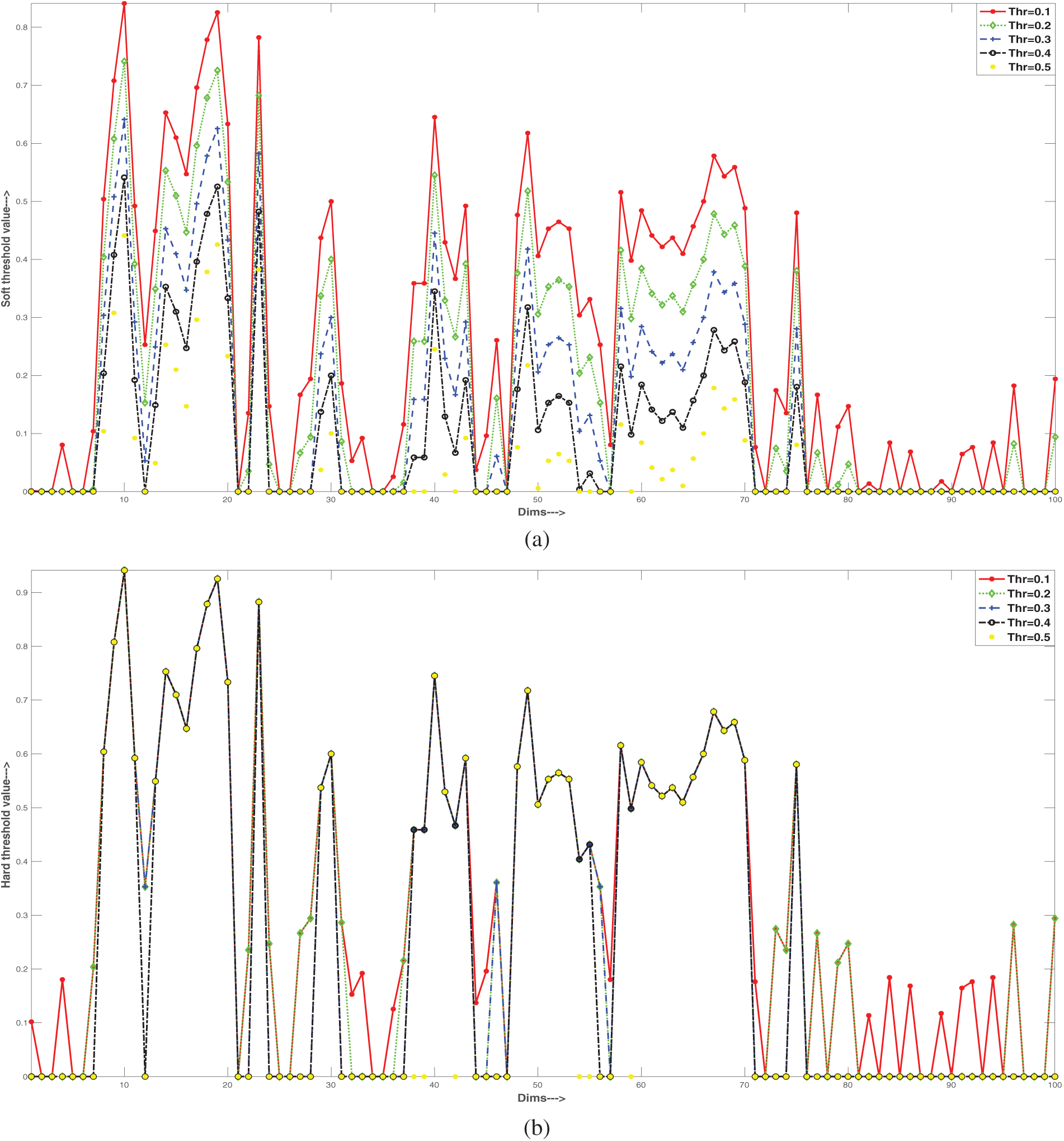
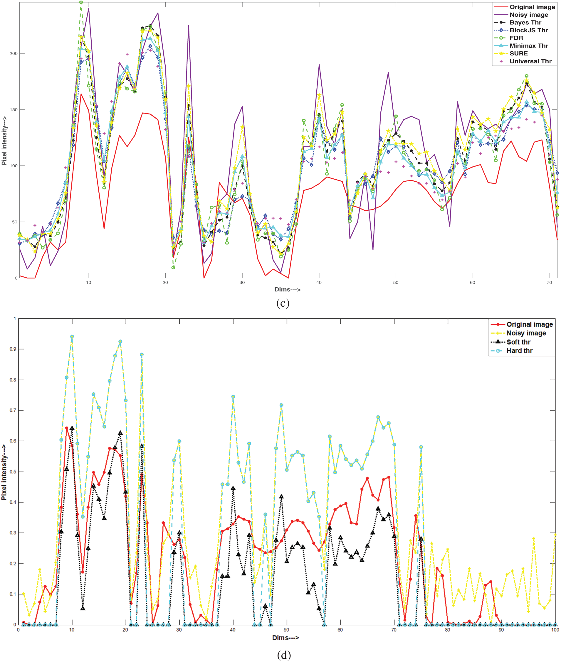
Figure 7: Graphical analysis of various thresholding techniques. (a) Variation of Soft thresholding with thresholding level. (b) Variation of Hard thresholding with thresholding level. (c) Variation in pixel intensities with various kind of thresholds. (d) Variation in pixel intensities with hard and soft thresholds
Table 6 summarizes the various thresholding techniques used for image denoising.
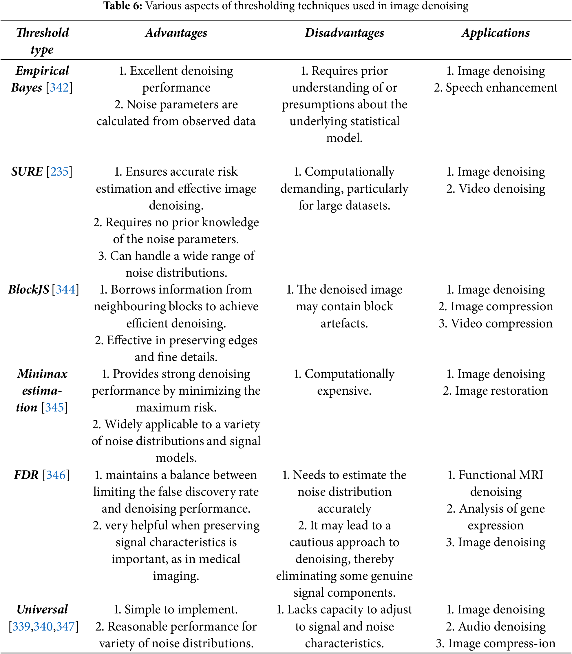
5 Image Noise Models and Artifacts
To simulate and examine the impact of noise on images, medical imaging often employs three types of noise modeling, namely Gaussian, Poisson and Rician. Poisson noise is related to the randomness of photon counting, whereas Gaussian noise is a kind of random fluctuation that follows a normal distribution. On the other hand, Rician noise happens when the means of the signal and noise are non-zero. Researchers can develop algorithms and approaches to efficiently mitigate or eliminate the effects of various types of noise on medical imaging by understanding and precisely modeling these types of noise. Table 7 provides an insight into some basic properties of these noises.
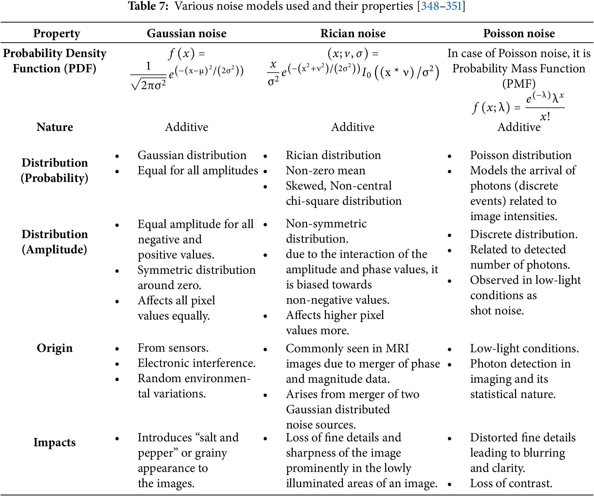
Fig. 8 illustrates the various artifacts commonly found in CT and MRI images. Magnetic resonance imaging (MRI) artifacts can result from the hardware of the MR scanner or a patient’s interaction with the device. Artifacts and foreign objects in the patient’s body might impair examination quality or be mistaken for a pathology. To prevent making incorrect diagnoses and learn how to eliminate them, understanding the artifacts and their origins is crucial. The medical history of patients is largely unknown to radiologists. Radiologists may struggle to distinguish between diseases and artifacts due to a lack of information. Artifacts can also be caused by specific patient circumstances, such as metallic implants or movement during the scan. To properly identify and reduce these abnormalities, radiologists must keep current on the most recent methods and MRI technological developments. It is important to note here that while acquisition level artifacts are modality specific, the post-processing artefacts are similar for both the modalities (Fig. 8) [352–355].
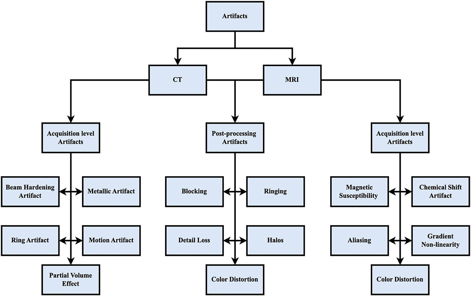
Figure 8: Block diagram showing various artifacts found in CT and MRI images
Denoising techniques as the basis of image fusion
Denoising techniques play a pivotal role in multi-modality medical image fusion. This field aims to combine information from various imaging modalities, such as magnetic resonance imaging (MRI), computed tomography (CT), and positron emission tomography (PET), to enhance the overall quality and information content of medical images. The success of image fusion heavily depends on the quality of the input images, and denoising is a crucial pre-processing step in this context. Through denoising techniques images are broken down into their coarser and finer versions, allowing for noise reduction while preserving important details. This is especially important in fusion techniques as noise can negatively impact the accuracy and clarity of the final fused image. Denoising techniques, such as wavelet denoising and Gaussian filtering, play a crucial role in enhancing the signal-to-noise ratio and facilitating a more accurate fusion process. By reducing noise, denoising facilitates the fusion algorithm in combining the most relevant and reliable information from each imaging modality, ultimately leading to enhanced diagnostic capabilities and improved medical decision-making.
Assessment parameters play a very important role in the validation process of an image denoising algorithm. These parameters play a crucial role in maintaining the integrity of image fidelity. Through meticulous parameter selection and precise calibration, researchers and developers can guarantee the optimal performance of the denoising algorithm across a diverse spectrum of images and noise intensities. Table 8 summarizes the various assessment parameters.

While using the metrics like PSNR and SSIM it is also crucial to consider the validation strategies. Some studies employed hold-out validation or k-fold cross-validation to ensure that denoising performance was similar across multiple data subsets. Moreover, model robustness is also an important but less-researched aspect of medical image denoising. Due to differences in scanners, acquisition protocols, and patient motion, clinical images often exhibit all manner of noise patterns under practical conditions. Some methods exhibited greater adaptability in handling such uncertainty, particularly ones that employed deep learning as well as sparse representation. However, many strong methods that perform well with simulated noise may fail in certain real-world noise distributions. These deviations should not influence a robust denoising method, as it should also generalize across unseen noise conditions. Model robustness estimation could be strengthened by using diverse collections of data, including clinical and publicly available images with varying amounts of noise. Table 9 summarizes the datasets that are used in image denoising.
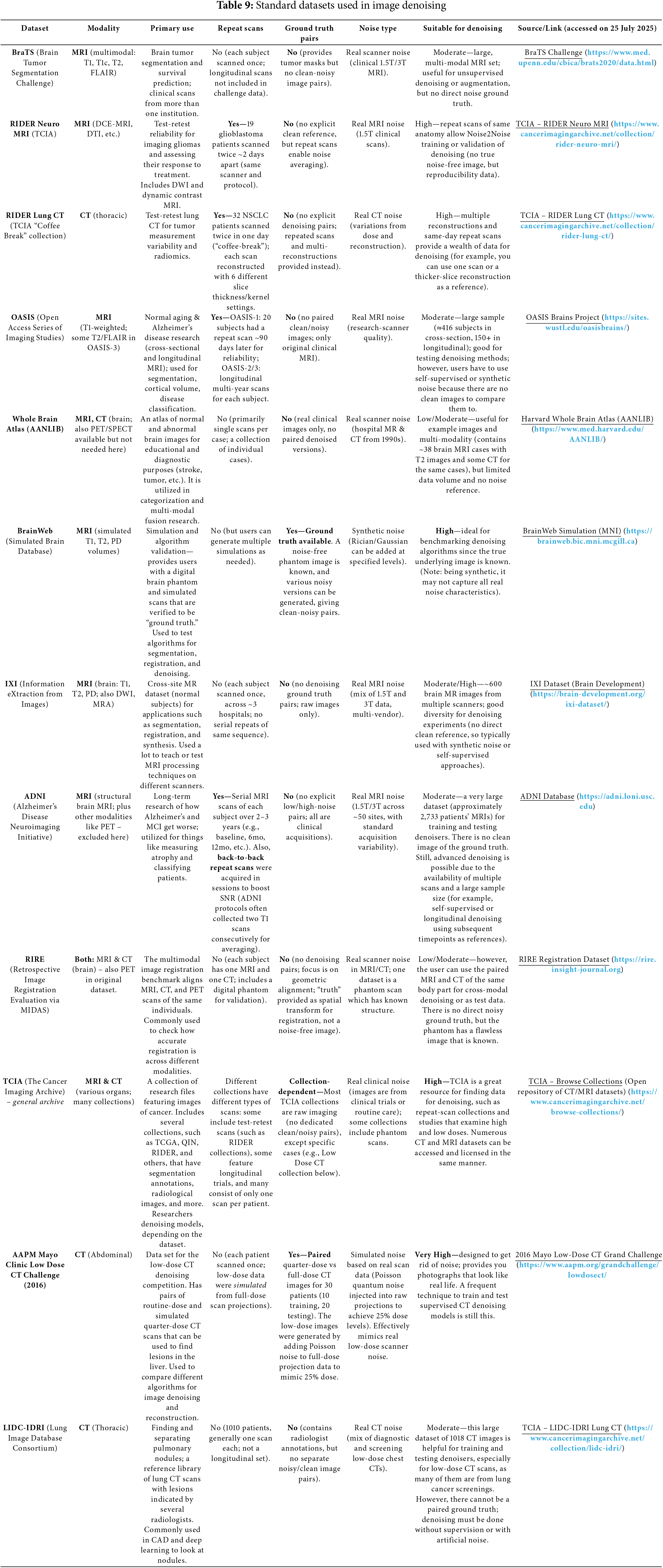
7 Experiments, Results and Discussions
We have performed the experiments on a single prime dataset of images, specifically an MRI image. The MRI image frame has been extracted from the raw images available at the Harvard Whole Brain Atlas (https://www.med.harvard.edu/AANLIB/) (accessed on 25 July 2025). Three types of artificial noises are injected which have common occurrence in MRI images. These noises are Poisson, Rician and Gaussian. Two different variances of Gaussian noise (0.01 and 0.05) are studied to highlight the performance of different techniques under different circumstances for same noise type. As the basic properties of the noise are known, non-blind image denoising approach has been adopted to denoise images. The experiment is performed by using MATLAB R2018b on a system equipped with an Intel Core i7 processor (2.6 GHz, 16 GB RAM) and running Windows 10.
We have tested 80 different method on these test images. These techniques (in the same order as graphs) are: Mean (Mean or Average filter), Binomial filter,
Fig. 9 illustrates the input images that are used in experiments. (a) This is the clean image, (b) gaussian noise of 0.01 variance, (c) gaussian noise of 0.05 variance, (d) poisson noise, and (e) rician noise. These techniques fall under specific categories of image denoising techniques depicted in Fig. 3. Both subjective and objective aspects of assessment are discussed to present a thorough picture of image denoising paradigms. The objective assessment of the results is done using parameters discussed in Table 8. Presenting tabled values would not be feasible due to a large number of values so we have presented the results in graphical form. Also, due to large range of values, the Logarithmic scale is used for the representation to present a relative picture of results.

Figure 9: Images under study (a) Original noise-free source image and original image infected with (b) Gaussian noise of 0.01 variance (Imrg1), (c) Gaussian noise of 0.05 variance (Imrg5), (d) Poisson noise (Imrpoi) and (e) Rician noise (Imrri or Imrrician)
Figs. 10–13 illustrate the denoising visual results of various techniques for dataset Imrg1, Imrg5, Imrpoi, and Imrrician respectively. The notations for dataset are kept according to the properties of the image and the type of noise present in them for instance Imrg1 represents an MRI image with Gaussian noise of 0.01 variance, Imrg5 represents an MRI image with Gaussian noise of 0.05 variance, Imrpoi represents an MRI image with Poisson noise and Imrrician represents an MRI image infected with Rician noise. For the sake of minimalism, we have incorporated visual results of few very important and best performing denoising techniques. To compensate a detailed statistical study of the results have been done and included in this review.

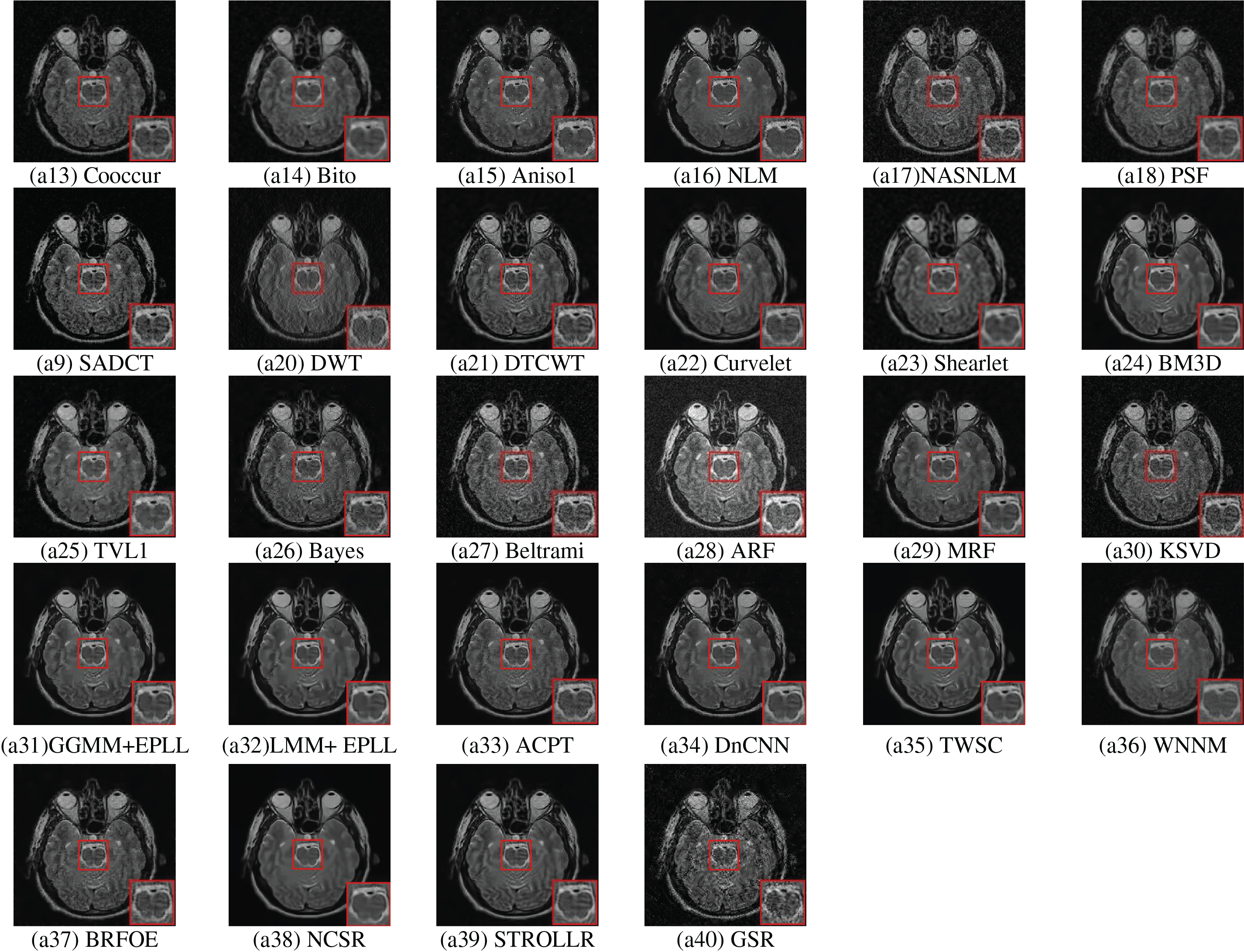
Figure 10: Denoising visual results of various techniques for Imrg1 (MRI image infected with Gaussian noise of 0.01 variance) image
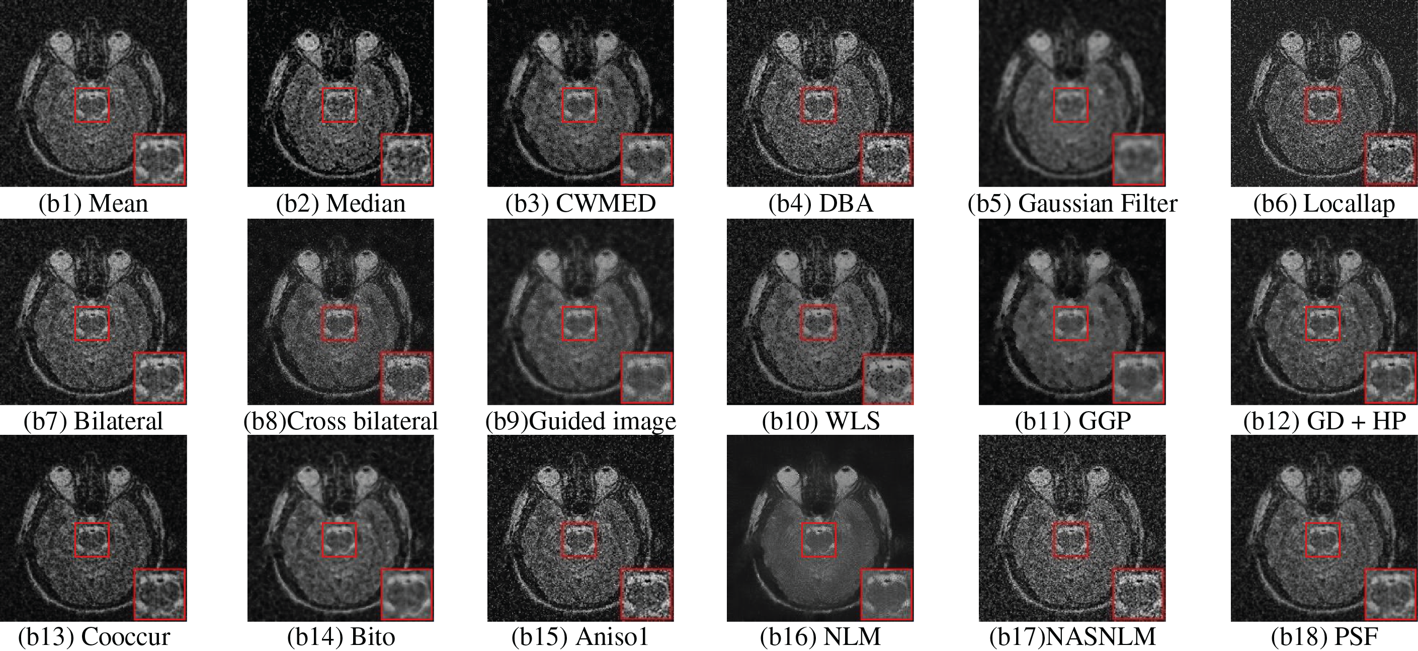

Figure 11: Denoising visual results of various techniques for Imrg5 (MRI image infected with Gaussian noise of 0.05 variance) image


Figure 12: Denoising visual results of various techniques for Impoi (MRI image infected with Poisson) image
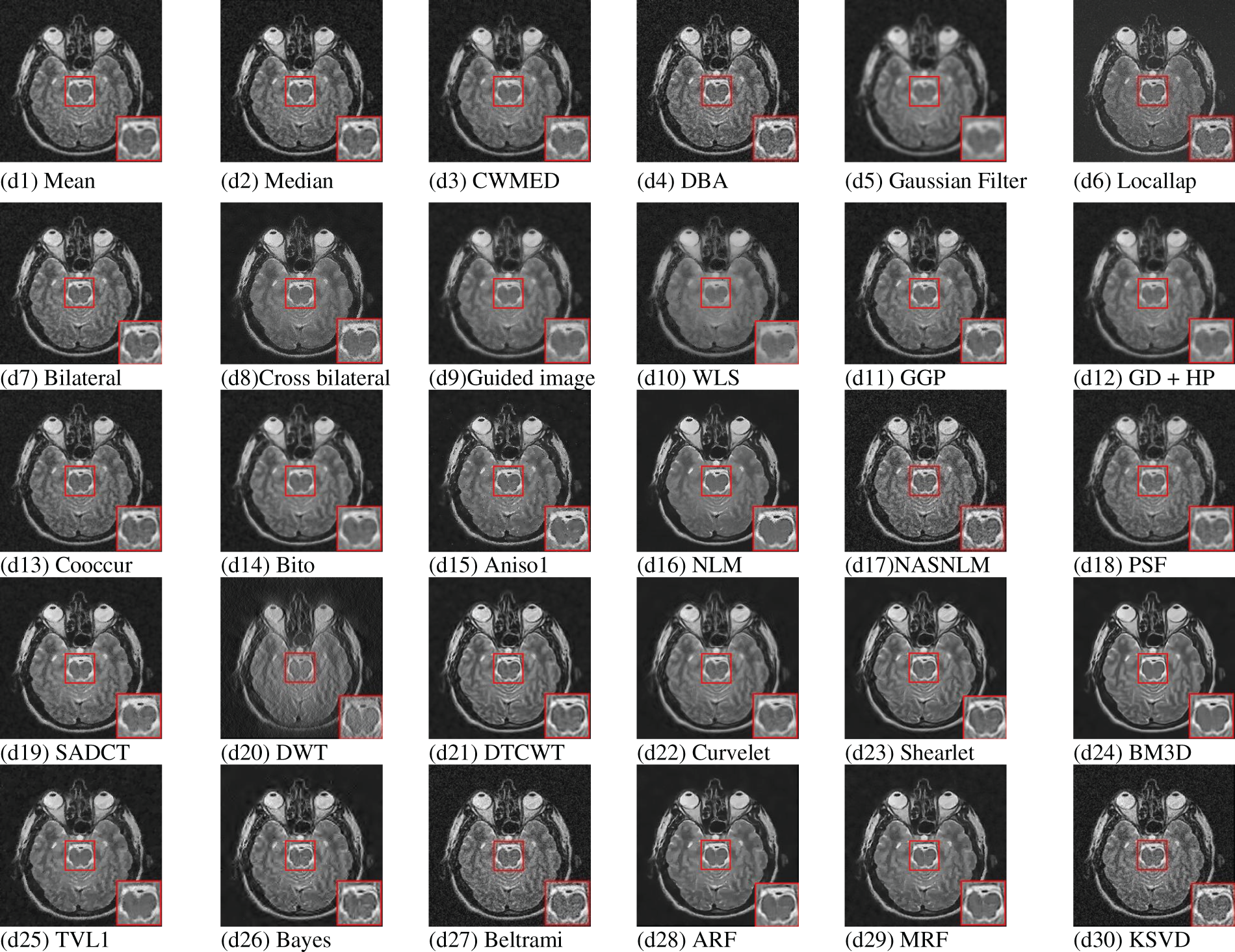
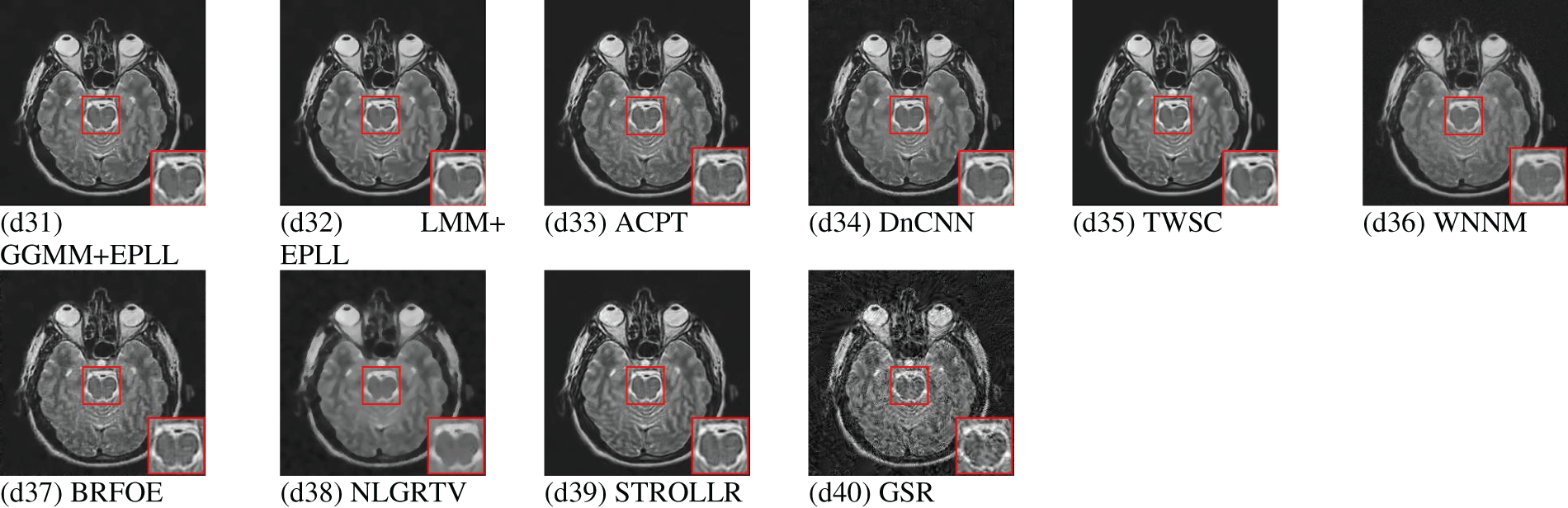
Figure 13: Denoising visual results of various techniques for Imrri (MRI image infected with Rician) image
The visual observations reveal some key points regarding qualitative comparison of various denoising methods:
a. The basic spatial filtering (mean, median, bilateral filter, etc.) work fairly in the case of low noise. As the intensity of the noise increases, these filters exhibit poor results both visually and objectively on assessment parameters.
b. The same conclusion (as in (a)), can be applied to miscellaneous filtering techniques, X-lets and even sparse based and patch-based techniques. They completely distort the image further making them devoid of any useful details.
c. The Low rank representation techniques like STROLLR, adaptive clustering techniques like ACPT, some sparse coding based denoising techniques and even some X-lets work well on low level Gaussian noise infected images.
d. The techniques like NLM, STROLLR, BM3D and most of the X-lets completely smoothen (including all edges and textures) the high intensity noise infected images.
e. Rician noise, due to is peculiar characteristics is very difficult to remove. We observed that in the case of Rician noise X-lets perform fairly well. Perhaps the shrinkage algorithms are effective in tackling such noise.
f. Most of the techniques worked well for Poisson noise. Some of the techniques are able to remove this noise without losing any significant details. It can also be seen that denoising techniques, in case of Poisson noise tends to affect the overall image brightness (as compared to Rician noise), in case of Beltrami regularization and MRF based denoising only, the image brightness increases.
g. As usually, the X-lets introduce ringing artifacts into the denoised image. The effect of these artifacts become more profound when the noise intensity increases. Therefore, as seen from above results, the artifacts are more profound in case of Imrg5 denoised image datasets.
h. Sparse and Low rank representation-based methods perform well on nearly all types of noise.
The Pons area of the axial view has been highlighted for all the images and from the first basic observation it is quite clear that the high levels of noise is still a standing problem even for some of the most sophisticated denoising algorithms. First of all, in case of noise infected images, the pons area is severely affected. The Basilar artery is totally invisible in image with high noise level and partially visible in other types (low level) of noises. The right and left globes are the areas still visible but even they are severely affected by high levels of noise.
In case of low levels of Additive White Gaussian Noise (AWGN), spatial filters and the X-lets were unable to properly restore the Basilar artery, the parts below the Vermis area. The techniques like DnCNN, TWSC and NCSR are able to provide near perfect restoration but significant details has been lost in the process. The classic techniques like NLM and BM3D have also provided good results but some techniques like GSR are not able to remove the noise up to the desired levels.
The case of high levels of Additive White Gaussian Noise (AWGN) is complex and challenging. While most of techniques failed drastically to preserve even the large structures and textures, some of the techniques like BM3D, DnCNN, NCSR and TWSC are able to restore the Basilar artery. Ringing artifacts are very prominent in the images denoised using X-lets and some techniques removed very small amounts of noise from the images. Some of the areas are completely removed and images are damaged to the extent where no meaningful information can be deducted.
The Poisson noise affects the image very differently. The first challenge to tackle this type of noise is that it is not uniform. The lack of uniformity makes it difficult to deal with. The edge preserving spatial filters seem effective in this case. While BM3D performed well result from NLM filter are not satisfactory. For X-lets, DTCWT perform fairly good while the others distort the image. The Rician noise seems very similar to the low level Gaussian noise visually. The results are also evident of this fact and the techniques perform equally good on Rician noise affected images.
Fig. 14 illustrates the values of various assessment papameters like (a) contrast, (b) coorelation, (c) dissimilarity, (d) energy, (e) entropy, (f) PSNR, (g) MSE, (h) SSIM for different denoising techniques (Represented on a Logarithmic scale).


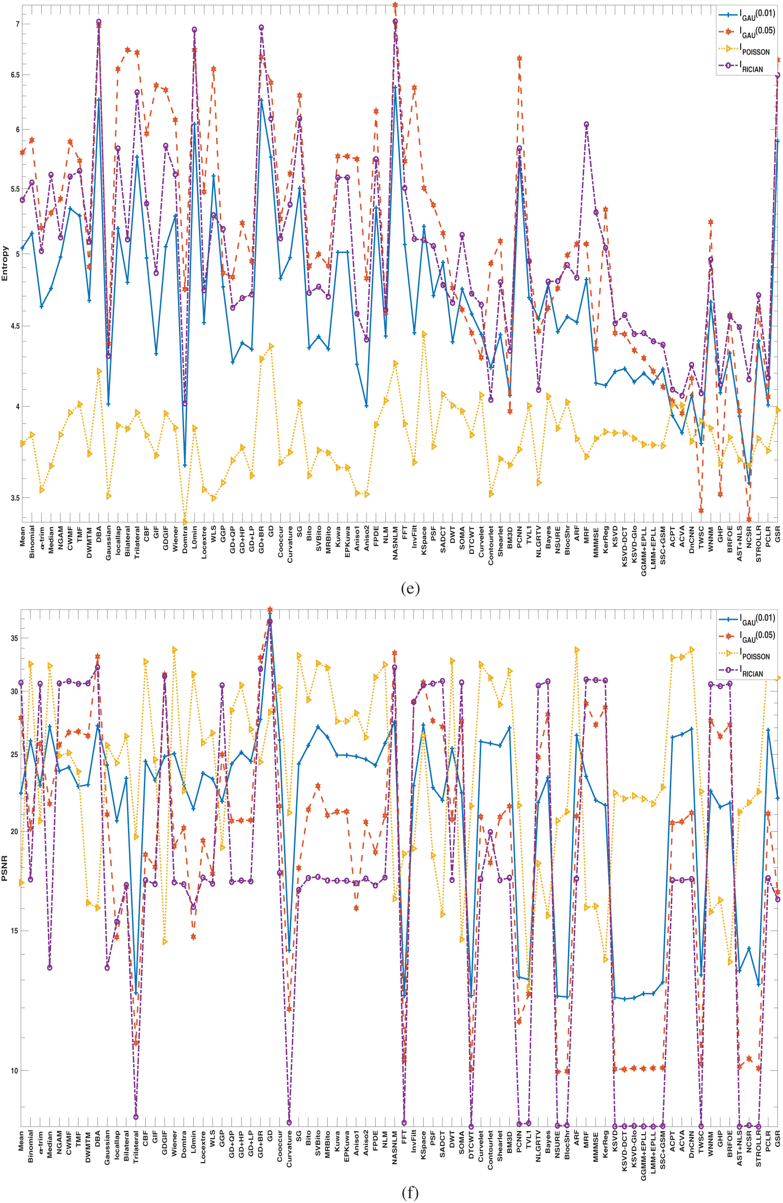
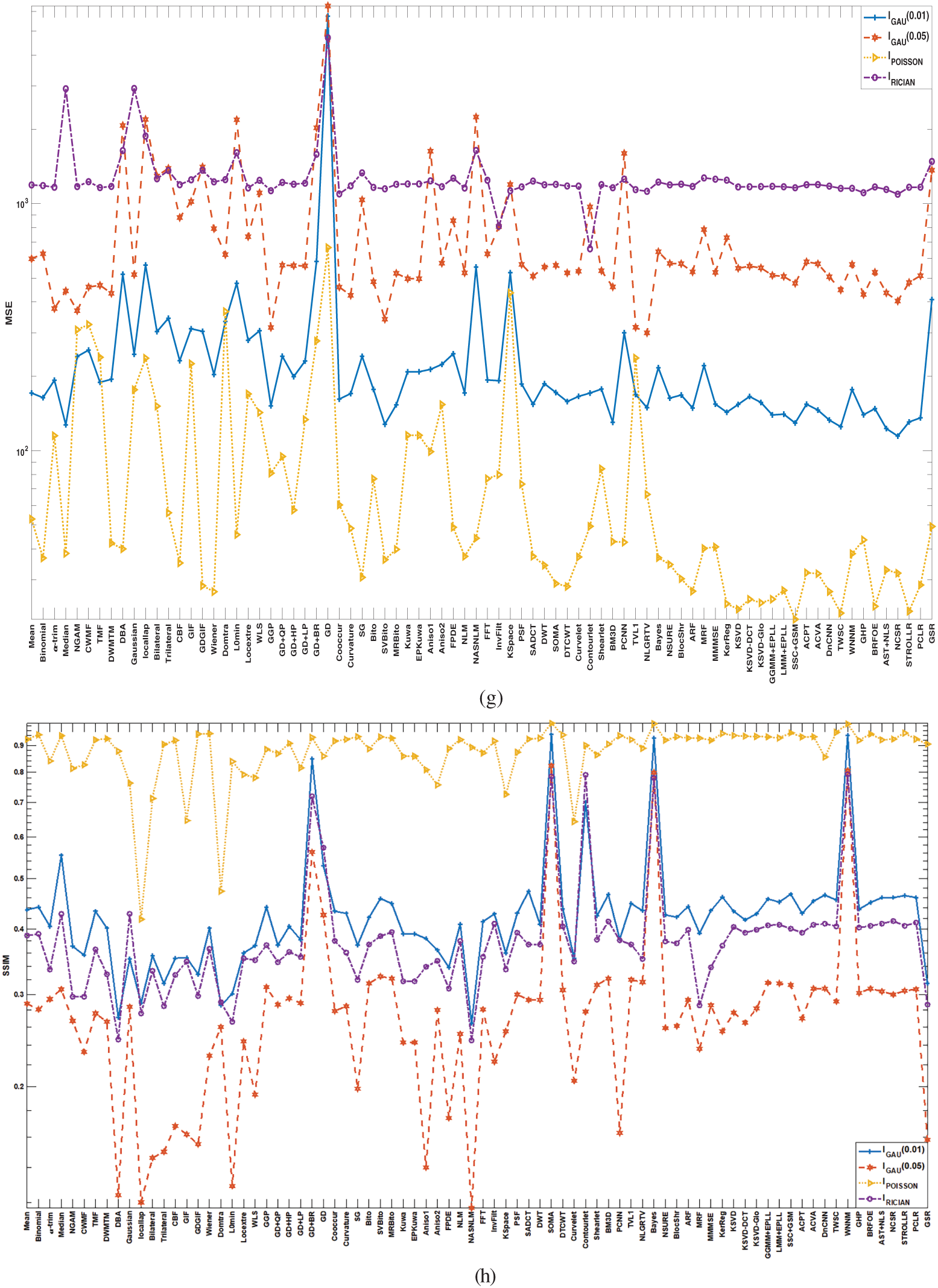
Figure 14: Values of various assessment papameters for different denoising techniques (Represented on a Logarithmic scale)
Table 10 summarizes the strengths and weaknesses of various denoising techniques.
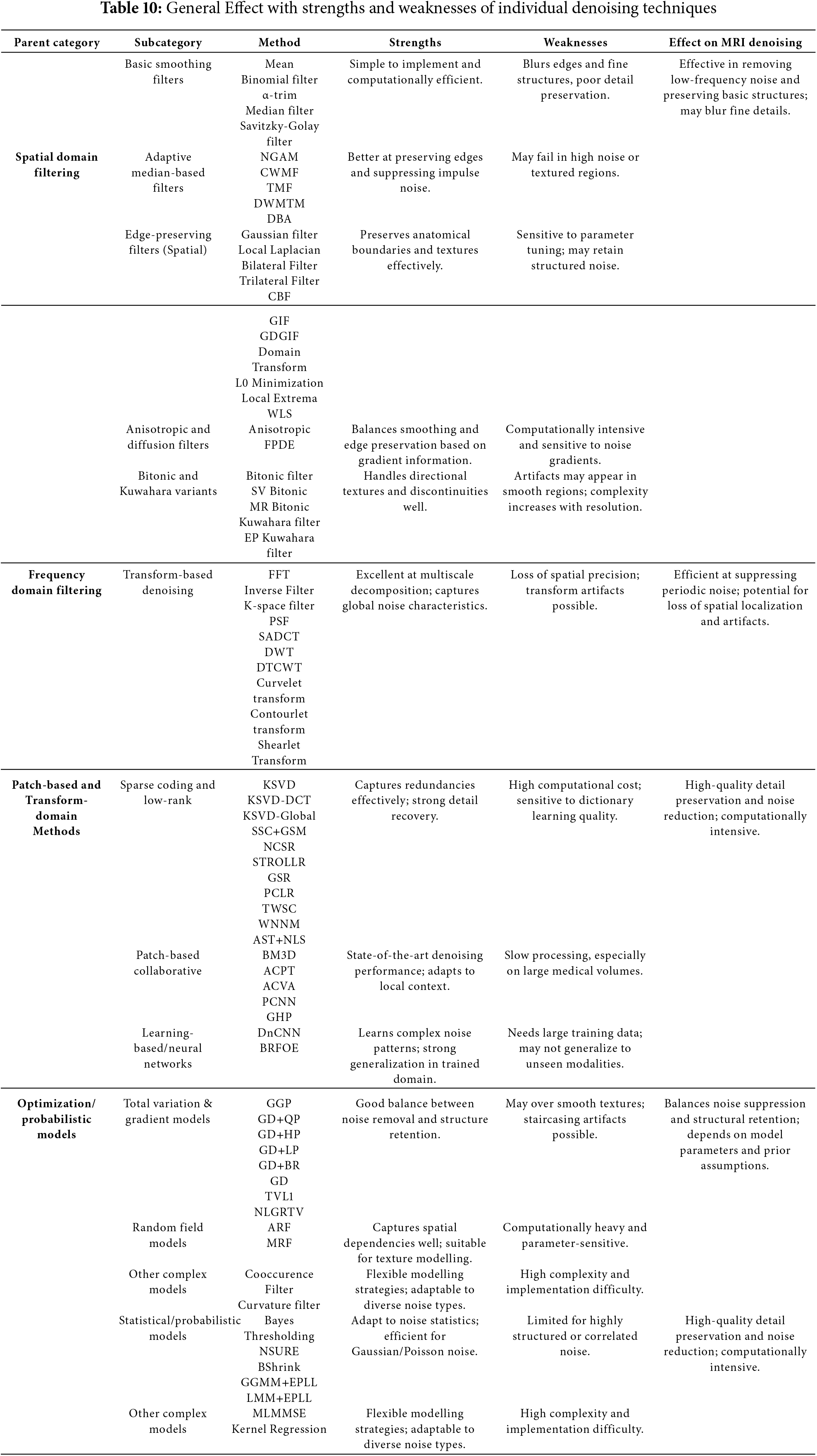
Tables 11–14 summarize the top five performing techniques for different input image dataset.
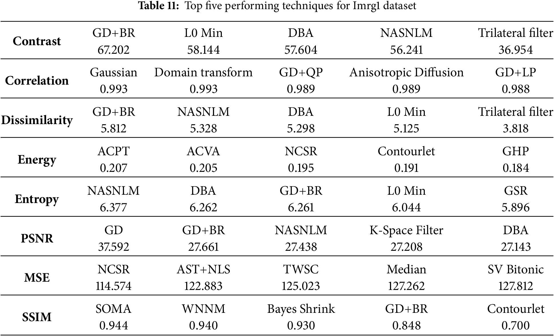
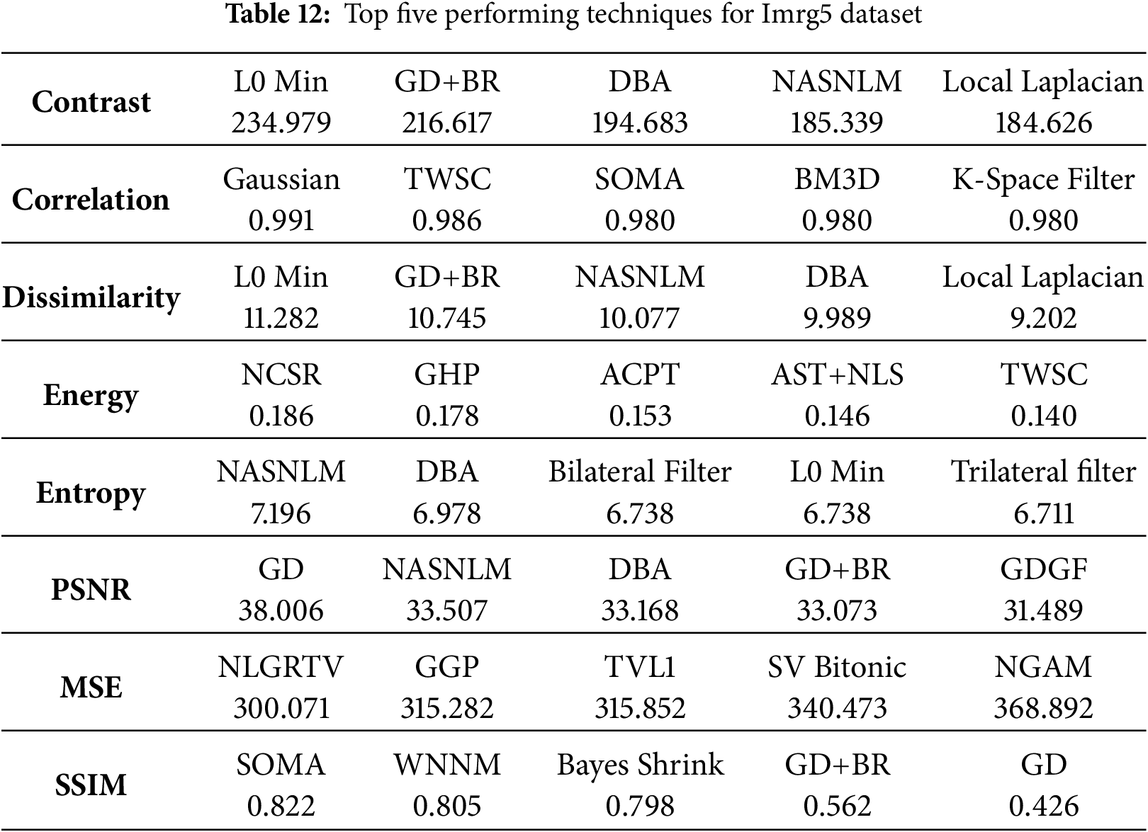
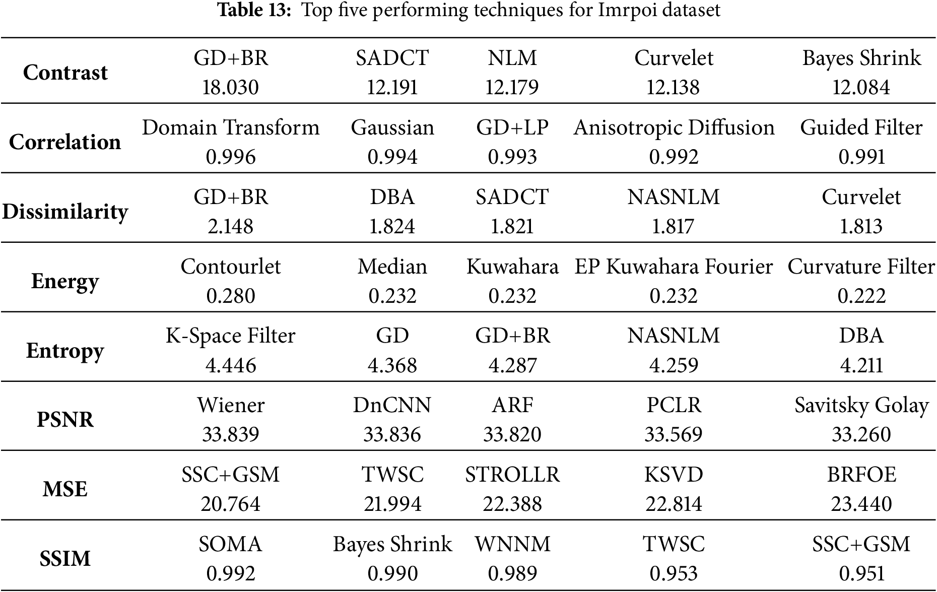
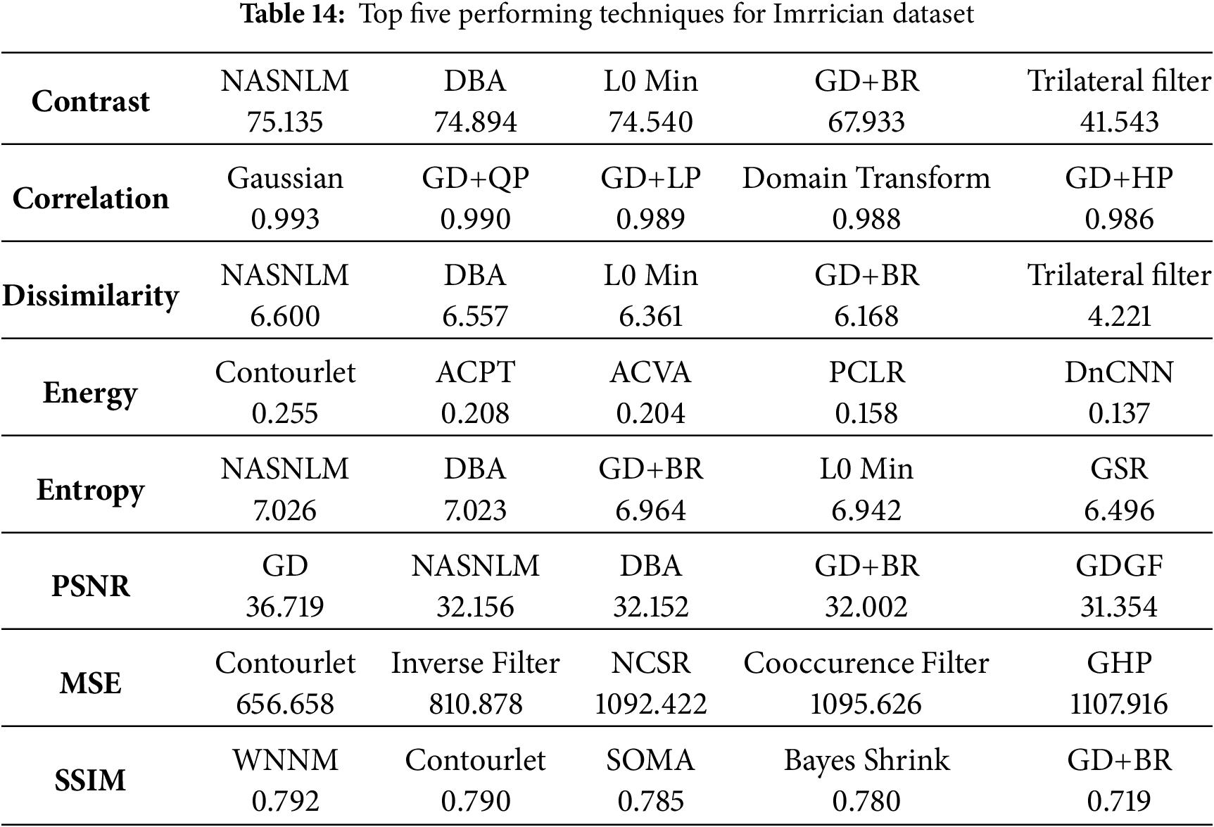
Tables 9–13 reveal some interesting quantitative insights like:
a. The only family that ranks highest on the Contrast-and- PSNR lists in all four noise levels is Edge-prior gradient-descent (GD + Beltrami/L0-minimization).
b. Always in the top for Dissimilarity, Entropy and PSNR, NASNLM (noise-adaptive NLM) is the most “texture-friendly” method available everywhere. If radiologists appreciate real tissue granularity, NASNLM is the best single option.
c. Under all noise types (Gaussian/Poisson/Rician conditions), DBA (decision-based adaptive median switch) ranks in the top-5 in Contrast, Dissimilarity, Entropy and PSNR—making it the best classical, CPU-light all-rounder.
d. Although they fall out of the top tier for Rician, SV-Bitonic/Trilateral/Local-Laplacian outrank other spatial kernels for Gaussian noise, therefore proving that directional bitonic kernels cope with additive blur better than multiplicative bias.
e. Low-rank & sparse patch methods (WNNM, TWSC, SSC+GSM, STROLLR, NCSR, PCLR) rule MSE and SSIM tables in every circumstance; they are statistical accuracy champions and should be selected when radiomics, segmentation or quantitative biomarkers follow denoising.
f. Under Rician and Poisson, transform-domain multiscale bases (Contourlet, Curvelet, Shearlet, SADCT) shine in MSE; otherwise, they win the Energy metric if smoothing homogeneity is sought. In the worst (Rician) situation, contourlet in particular is the only way to top Energy, MSE, and SSIM concurrently.
g. Wiener is still a PSNR leader for Poisson noise, demonstrating that, after variance stabilization, classical linear filters are still important when noise is almost Gaussian.
h. Although it never ranks in any other metric, pure Gaussian filters always lead raw correlation, therefore highlighting the trade-off between simple smoothing and diagnostic accuracy.
a. Visual-emphasizing techniques → GD+BR or NASNLM (high Contrast/Entropy, adequate SSIM).
b. Quantitative analytics → WNNM/TWSC/NCSR (best SSIM-MSE pair, consistent across all noise models).
c. Mixed contexts → DBA or NASNLM (consistent top-5 presence across all metrics without GPU demand).
d. Gaussian 0.01 → edge hyper sharpeners give record PSNR (GD 37 dB); Gaussian 0.05 → low-rank TWSC/WNNM start to outscore GD in SSIM and MSE; Poisson → Wiener and
e. DnCNN co-lead PSNR; sparse methods keep SSIM ≥ 0.99; Rician → Contourlet + WNNM pair yields the lowest error, NASNLM keeps texture.
f. Algorithms that top Entropy (NASNLM, GD+BR) seldom top Energy, and vice-versa (Contourlet, ACPT) see entropy against energy seesaw. Choose based on the goal whether flatness or texture retention.
g. CNN (DnCNN) never tops a metric list except PSNR (Poisson), but it is always mid-top-10 in every measure—robust plug-and-play alternative when GPU resources exist and parameter tinkering is unwanted.
h. Confirming its strength when noise is spatially variable, gradient domain guided filter stealthily enters PSNR top-5 in both Gaussian 0.05 and Rician.
i. At least three of the five greatest SSIM scores in every table come from low-rank/sparse-representation techniques, therefore highlighting the statistically rather than heuristically driven nature preservation in every table.
j. For a fast, high-contrast preview layer, GD+BR or L0-min are useful; NASNLM for clinical reading; WNNM/TWSC for quantitative pipelines and Contourlet for severe Rician.
k. Integrate a sparse/low-rank denoiser (WNNM, TWSC, NCSR) directly before texture-feature extraction; these retain SSIM and cut MSE, thus radiomic fingerprints remain constant between scanners and sessions.
7.2 Result Synthesis and Analysis
In this section, the techniques are divided into six broader categories to get a general idea of the performance of techniques belonging to each of these categories. It is important to note here that inter-category performance varies a lot compared to intra-category performance.
1. Spatial Domain Filters
Examples: Mean, Median, Binomial, Harmonic, Alpha Trim, DWMTM, etc.
These filters are easy to understand, and they work really well, especially with PSNR. Adaptive median filters and harmonic versions likely assisted helped in a good way. Best for rapid modifications or real-time preprocessing pipelines where speed is more important than getting everything right.
Insights:
• Basic filtering approach that operates directly on image pixels using sliding windows (kernels).
• Strengths:
∘ Easy to implement, fast, computationally light.
∘ Good for removing impulse noise (salt & pepper) and mild Gaussian noise.
• Limitations:
∘ Non-adaptive: applies same filter across all regions, leading to edge blurring.
∘ Not effective at preserving fine details or textures.
• Performance:
∘ Generally lower PSNR/SSIM compared to advanced methods.
∘ Median variants perform better than mean filters in high-noise scenarios.
Use When:
Quick, real-time or low-resource denoising is required, and edge precision is not critical.
2. Transform Domain Methods
Examples: Wavelet, Curvelet, Contourlet, Fourier, Gabor, TWSC, GHP, etc.
These approaches are great at maintaining structure (best SSIM), because they use multi-scale representation. But to keep things consistent, they prefer to hide small pixel changes, which can make the PSNR a little lower. Best for medical imaging, texturing, and outputs that are easy to compress.
Insights:
• Transform the image into another domain (frequency/multiscale), perform noise suppression, then inverse-transform.
• Strengths:
∘ Multi-resolution: Efficient in preserving edges and fine textures.
∘ Can separate noise from signal more accurately than spatial filters.
• Limitations:
∘ Requires careful selection of thresholding strategies.
∘ Some transforms (e.g., Wavelets) may introduce artifacts if improperly tuned.
• Performance:
∘ Generally good balance between denoising and detail preservation.
∘ Wavelet-based methods (like BayesShrink, GHP) often outperform spatial domain methods on SSIM.
∘ Curvelet/Contourlet are excellent at capturing directional features (e.g., edges, ridges).
Use When:
High-frequency preservation is crucial—e.g., medical imaging, texture analysis, edge-sensitive tasks.
3. Patch-Based Methods
Examples: NLM, NASNLM, BM3D, CBM3D, WNNM, NCSR, STROLLR, GSR, etc.
These are reliable performers, especially when it comes to SSIM and visual quality, which is due to their patch-matching system. They are quite close to hybrid approaches, although they are better at keeping fine textures and adapting to non-linear noise. Ideal for removing noise from natural scenes and photographs with lots of patterns.
Insights:
• Exploit self-similarity in images by comparing and aggregating patches from different regions.
• Strengths:
∘ State-of-the-art denoising for many years (BM3D is a benchmark).
∘ Excellent detail preservation and structure-aware denoising.
∘ Adaptable to various noise models and noise levels.
• Limitations:
∘ Computationally expensive, especially for large images.
∘ Patch matching can fail in highly textured or uniform regions.
• Performance:
∘ Usually among top performers in PSNR and SSIM.
∘ WNNM, BM3D, NASNLM are especially strong on Gaussian noise.
Use When:
High-quality restoration is critical and computational resources are available (e.g., remote sensing, medical scans).
4. Gradient-Based Methods
Examples: GD, GD+BR
These approaches, such as GD and GD+BR, work very well for restoring structures, keeping edges and gradients even if there are some pixel-level errors (greater MSE). Great for technical and diagnostic imaging where, keeping the edges clean is more important than matching pixels.
Insights:
• Use gradient minimization or variational frameworks to enforce smoothness while preserving edges.
• Strengths:
∘ Edge-preserving and good at reducing blocking artifacts.
∘ Can be tuned for structure-aware denoising.
• Limitations:
∘ Performance is highly dependent on regularization parameters.
∘ May over smooth textures or introduce halo artifacts.
• Performance:
∘ In the dataset, GD dominates all in PSNR.
∘ Adding bilateral regularization (GD+BR) may trade off detail for smoothness.
Use When:
You want analytical control over the denoising process and need to preserve strong geometric structures.
5. Hybrid & Deep Learning Methods
Examples: DnCNN, AST+NLS, AST+TV, DBA, TV+Wav, BRFOE
These approaches do well on all measures in this dataset, but not the best. They produce outputs that look well and have a moderate amount of structural similarity, but they are not optimized just for PSNR or MSE. Best suited for natural images, facial reconstructions, and learning-based applications.
Insights:
• Combine spatial/transform methods with deep learning or advanced regularization (TV = Total Variation).
• Strengths:
∘ Deep networks like DnCNN learn adaptive, non-linear mappings from noisy to clean images.
∘ AST (Adaptive Smoothing Transform) methods adapt to local structures dynamically.
∘ TV methods are good for piecewise smooth areas (e.g., cartoons, medical).
• Limitations:
∘ Deep models require training data and, may not generalize to all noise types.
∘ TV-based methods may introduce staircasing or over-smooth regions.
• Performance:
∘ DnCNN and BRFOE perform consistently well on structural similarity (SSIM).
∘ Hybrid methods often balance spatial and spectral advantages.
Use When:
You need flexible, high-performance denoising—especially if training data is available or adaptivity is key.
6. Thresholding & Statistical Filters
Examples: Wiener2D, Adaptive Median, BayesShrink,
Insights:
• Rely on statistical modeling of noise or pixel relationships.
• Strengths:
∘ Target specific noise distributions (e.g., Rician for MRI, Gamma for speckle).
∘ Wiener filtering adapts based on local variance.
• Limitations:
∘ Not always flexible—performance drops if noise model is mismatched.
∘ Often outperformed by patch-based or transform methods in general scenarios.
• Performance:
∘ Useful as pre-processing or in conjunction with other methods.
∘ Good PSNR in uniform areas, but may lag in structure-sensitive metrics.
Use When:
Noise characteristics are known and match the statistical model used.
Final Takeaways:
• Patch-based and Hybrid/Deep methods are most powerful for general-purpose denoising. They not only shine more in visual quality but also in numerical fidelity.
• Gradient-based methods are excellent when edge preservation is crucial (e.g., structural imaging). They dominate the dataset, possibly because of their mathematical robustness and edge-focused optimization.
• Transform domain methods offer a solid mid-ground—good perceptual quality with relatively low computational cost.
Spatial and statistical filters are best for simple use-cases or as part of a hybrid pipeline.
7. General Statistical Observations from the Results
Some general or common observations which can be deducted from the descriptive statistic methods are:
a. The boxplots reveal that the effect of denoising techniques is resembling in case of images affected by gaussian noise (Imrg1) and Rician noise. The width of the boxes showing variability and the extent of the whiskers showing the range of the values is nearly same in case of all assessment parameters except PSNR. In case of PSNR, there is a visible difference in the boxplots of the two. This can be possibly attributed to the associated sensitivities of PSNR as a metric or the unique statistical properties of Rician noise.
b. Images affected by Gaussian noise of 0.05 variance is very hard to remove and all the denoising techniques produce unsatisfactory results both on subjective and objective scales.
c. According to visual results and the statistical analysis of all the metrics it is evident that all the denoising techniques perform well in the case of Poisson noise removal.
d. The restoration process works very well particularly in case of Sparse based and Patch prior based methods.
Based on the contrast values derived from the application of various techniques on four distinct datasets, has been shown in Fig. 15, it is evident that Imrg1 exhibits a minimum value of 0.87 (achieved through the utilization of domain transform filtering) and a maximum value of 67.2. Similarly, Imrg5 demonstrates a minimum value of 1.07 and a maximum value of 234.97, Imrpoi showcases a minimum value of 0.64 and a maximum value of 18.02, while Imrrician displays a minimum value of 1.48 and a maximum value of 75.13. The empirical evidence presented herein demonstrates that the magnitude of contrast values exhibits a substantial degree of variability across all examined test images, with the exception of the Imrpoi test images. The comparative analysis of image contrast, particularly in the presence of diverse noise types like Gaussian, Rician, or Poisson noise, frequently indicates a diminished contrast in images affected by Poisson noise.
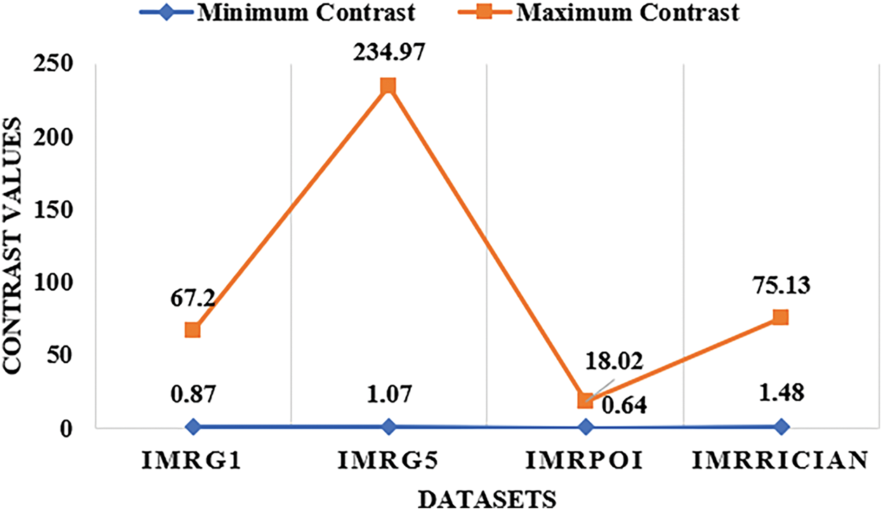
Figure 15: Minimum and maximum contrast values comparison of different datasets
There exist a multitude of elucidations for this phenomenon. Initially, it is important to acknowledge that Poisson noise exhibits a statistical distribution that is contingent upon the intensity of the signal. Consequently, in regions characterized by low intensity, the Poisson noise may exhibit a dominant presence, thereby diminishing the signal-to-noise ratio (SNR) and subsequently resulting in a reduction of apparent contrast. The perturbations induced by the inherent uncertainty of photon arrivals and the subsequent detection process, commonly associated with Poisson noise in photon counting methodologies, additionally impact the contrast, particularly in regions characterized by a low number of detected photons. Furthermore, when contrasting additive noise models such as Gaussian or Rician noise, it is noteworthy that the multiplicative nature of Poisson noise may yield a discernible visual perception of contrast. As a consequence of the shot noise characteristics of Poisson noise, which arise from discrete photon emission and detection, the presence of high-frequency variations leads to the alteration of minute details and texture, thereby causing a reduction in contrast.
The selection of appropriate noise reduction methodologies and algorithms can significantly impact the perception of contrast quality. In the context of mitigating Poisson noise, denoising algorithms may exhibit a propensity to assign greater importance to the reduction of noise rather than preserving subtle features, thereby leading to a perceptible decline in contrast. It is of utmost importance to maintain cognizance of the fact that the impact of auditory disturbances on the differentiation between luminance levels may undergo alterations contingent upon the specific visual stimuli, the inherent characteristics of the visual disturbances, and the idiosyncratic perceptual faculties of individual observers. The boxplot analysis demonstrates that the dispersion in the contrast values of the Imrg5 dataset is significantly elevated as a result of a substantial Inter Quartile Range (IQR), which is further corroborated by the visual outcomes of the denoising process.
In case of correlation, where all the values typically range from 0 to 1, the boxes are aligned to the right showing that most of the correlation results are very close to 1. Tables 15–18 summarize descriptive statistics for the denoising techniques applied on four different input image dataset.
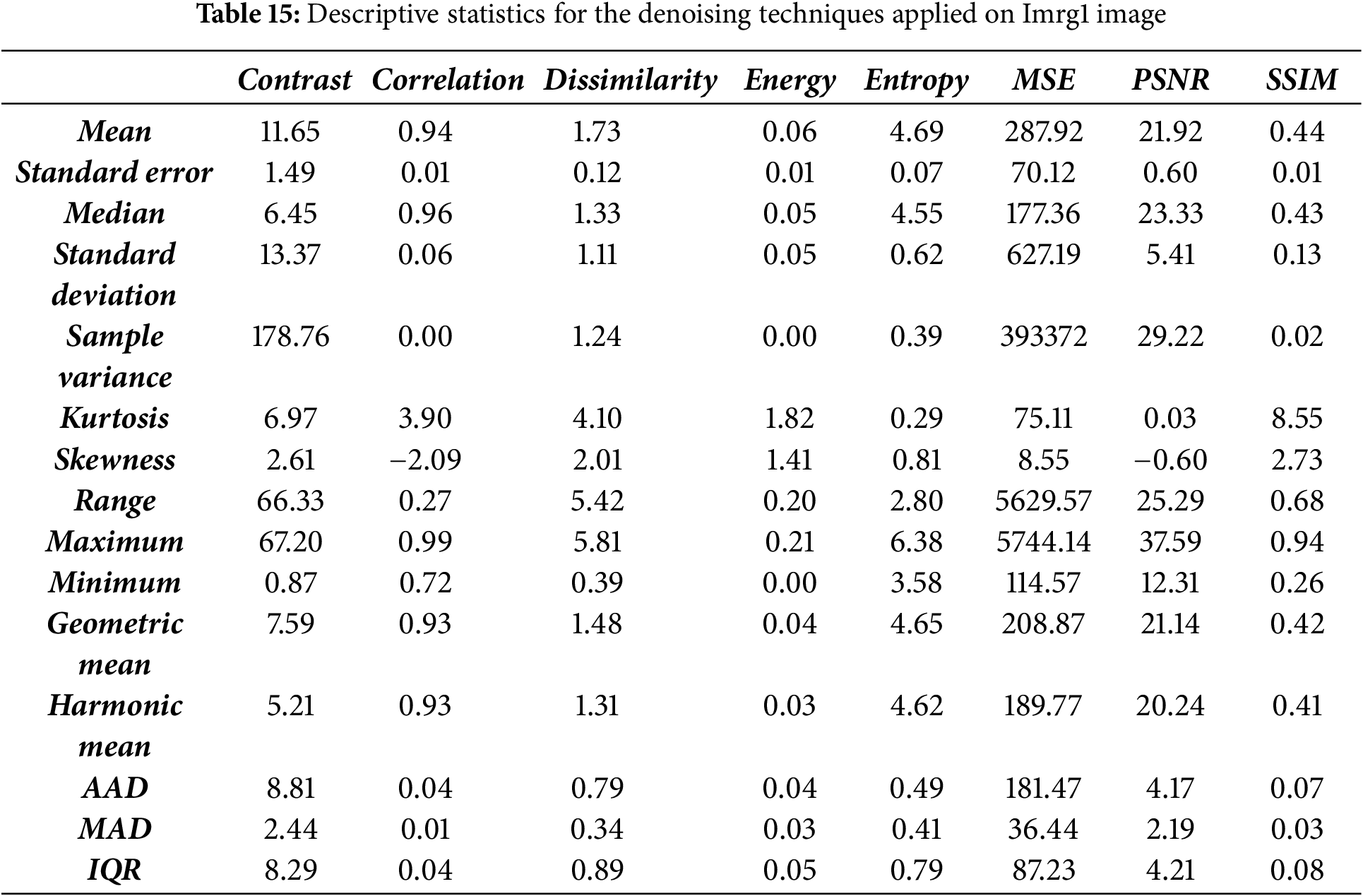
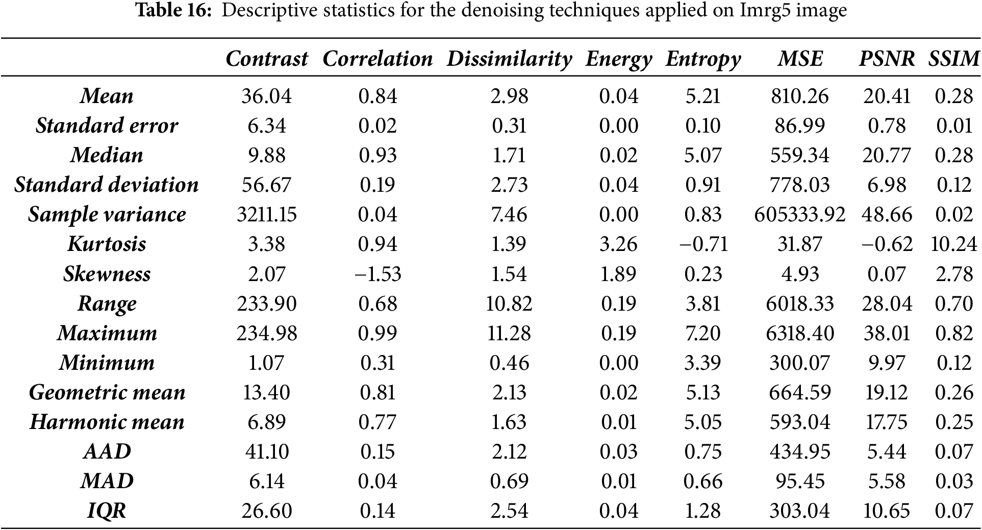
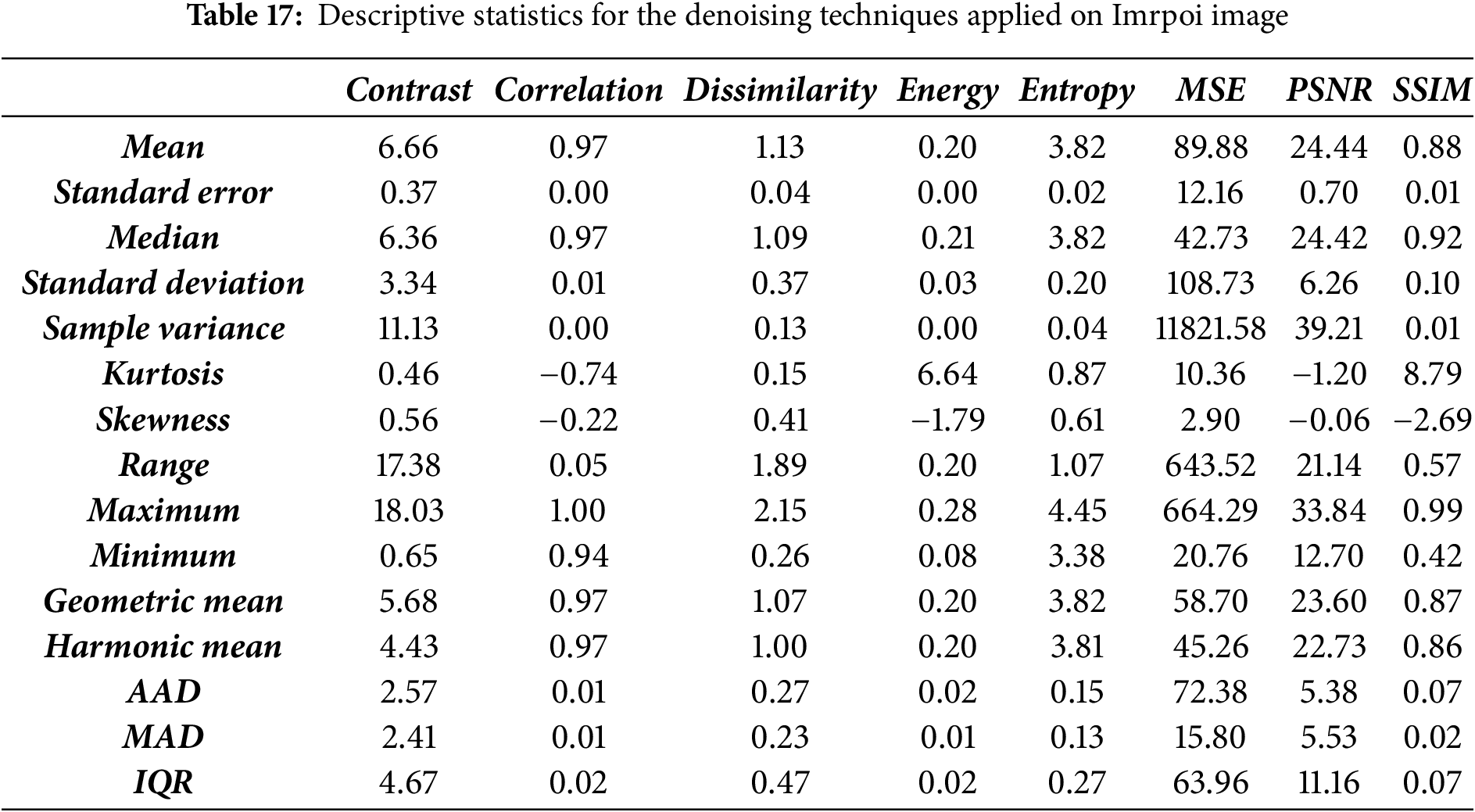
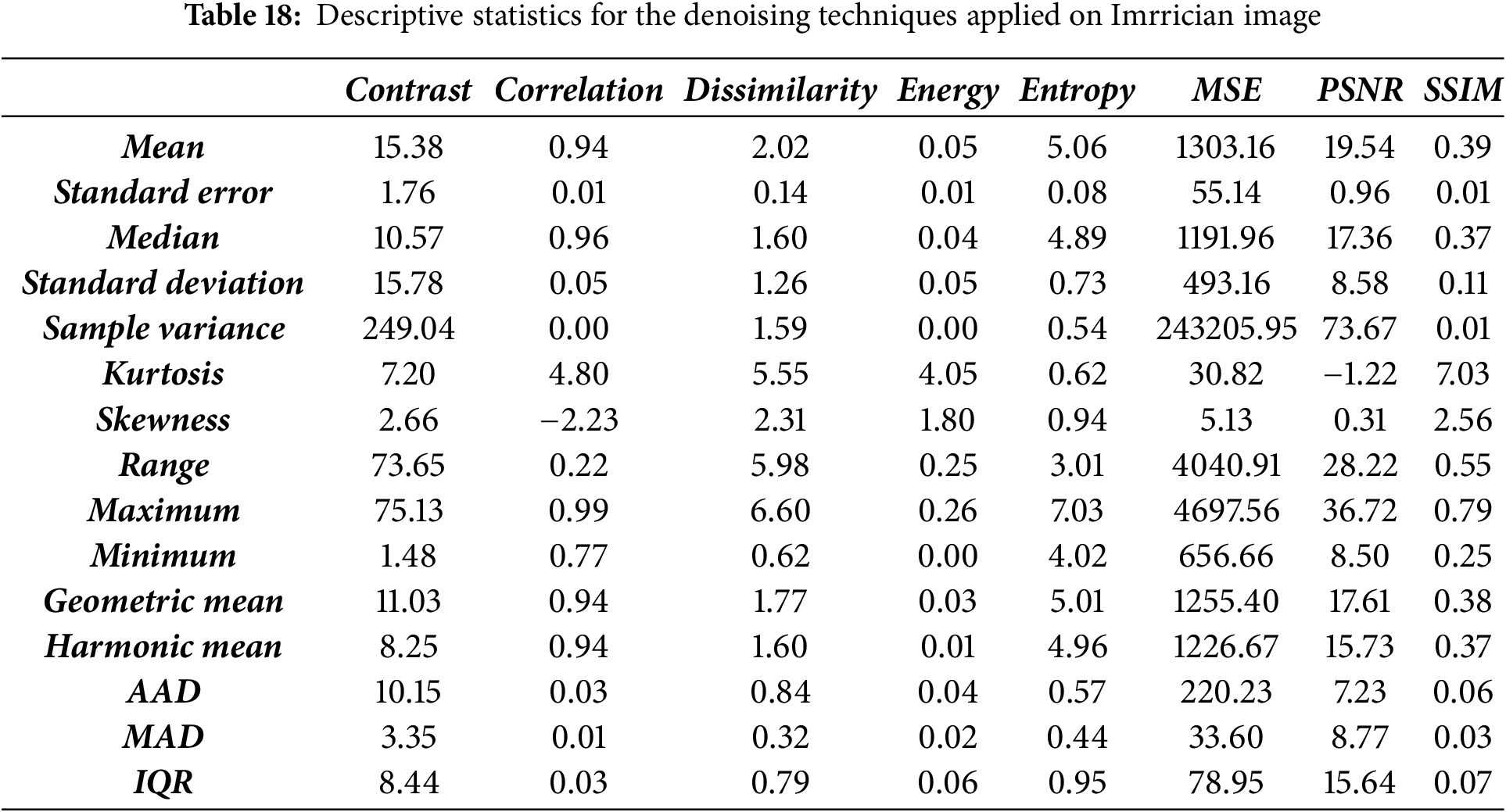
• For Imrg1 image:
1. The contrast value has standard error of 1.49 and MSE has standard error of 70.12. The large values of standard error indicate higher variability in the data. All other values of standard error are less than 1 indicating comparatively lesser variability. The parameters with lesser standard error, i.e., correlation, energy, entropy and SSIM exhibit higher precision and lesser noise.
2. The measures of variability and spread of the data viz. Range, Inter Quartile Range (IQR), Variance, Standard Deviation, Sample Variance (SV), Average Absolute Deviation (AAD) and Mean Absolute Deviation (MAD) also confirm that the variability is maximum in Contrast, PSNR and MSE making them comparatively lesser precise.
3. Although it is well established that Mean > Geometric Mean (GM) > Harmonic Mean (HM) the value of mean is not significantly larger.
4. The Kurtosis values for Contrast, MSE and SSIM are very high indicating more peaked or heavy-tailed data. More peaked data means the concentration of data points is more around the central value or peak and heavy-tailed means that the data have more extreme value or outliers.
5. The skewness value is negative for correlation and PSNR which means these two parameters’ values are skewed to the left. The skewness value for PSNR is very near to zero which indicates a near normally distributed data.
For Imrg5 image:
1. The contrast value has standard error of 6.34 and MSE has standard error of 86.99. The large values of standard error indicate higher variability in the data. All other values of standard error are less than 1 indicating comparatively lesser variability. The energy, entropy and SSIM have nearly 0 standard error. The other parameters with lesser standard error, i.e., correlation, dissimilarity and SSIM exhibit higher precision and lesser noise.
2. The measures of variability and spread of the data also confirm that the variability is maximum in Contrast, PSNR and MSE making them comparatively lesser precise. Additionally, dissimilarity and PSNR also have significant variability.
3. Although it is well established that Mean > Geometric Mean (GM) > Harmonic Mean (HM) the value of mean is not significantly larger except contrast and MSE.
4. The Kurtosis values for contrast, energy, MSE and SSIM are very high indicating more peaked or heavy-tailed data. This value is significant in the case of dissimilarity also and observed negative for entropy and PSNR. More peaked data means the concentration of data points is more around the central value or peak and heavy-tailed means that the data have more extreme value or outliers. On the other hand, the data having negative kurtosis value (entropy and PSNR) is platykurtic i.e., flat peaked with comparatively lesser outliers.
5. In this case the skewness is negative for correlation and very less (but positive) for entropy and PSNR. Negative skewness means that the data is aligned towards the right.
For Imrpoi image:
1. The contrast value has standard error of 0.37, MSE has 12.16 and PSNR has 0.7. The large values of standard error indicate higher variability in the data. All other values of standard error are very less (below 0.05) indicating comparatively lesser variability. The energy and correlation have nearly 0 standard error. All the parameters with lesser exhibit higher precision and lesser noise.
2. The measures of variability and spread of the data also confirm that the variability is maximum in Contrast, PSNR and MSE making them comparatively lesser precise.
3. The value of mean is not significantly larger than geometric mean and harmonic mean except MSE.
4. The Kurtosis values for energy, MSE and SSIM are very high indicating heavy-tailed data. It is negative for correlation and PSNR indicating lesser tails or outliers. Contrast, dissimilarity and entropy have less but positive value of kurtosis showing moderate tails.
5. The value of skewness is negative for correlation, energy, PSNR and SSIM. Also, it is very less (but positive) for contrast, entropy and dissimilarity plus MSE has a large skewness value. Negative skewness means that the data is aligned towards the right and vice-versa.
For Imrrician image:
1. The contrast value has standard error of 1.76, MSE has 55.14 and PSNR has 0.96. The large values of standard error indicate higher variability in the data. All other values of standard error are very less indicating comparatively lesser variability. The energy, SSIM and correlation have nearly 0 standard error. All the parameters with lesser standard error exhibit higher precision and lesser noise.
2. The measures of variability and spread of the data are consistent with earlier results and confirm that the variability is maximum in Contrast, PSNR and MSE making them comparatively lesser precise.
3. The value of mean is not significantly larger than geometric mean and harmonic mean except Contrast, MSE and PSNR.
4. The Kurtosis values for all the parameters are high except entropy indicating heavy-tailed data. It is negative for PSNR indicating lesser tails or outliers.
5. The value of skewness is negative for only correlation. Also, it is less but positive for entropy and PSNR. Additionally, MSE has a large skewness value.
Fig. 16 shows the error analysis of different datasets by using the standard error and MSE. It emonstrates a comparison of Mean Squared Error (MSE) vs. Standard Error on four different MRI datasets with diverse types and intensities of corrupting noise. The datasets are contaminated with Gaussian noises of variances 0.01 (Imrg1) and 0.05 (Imrg5), Poisson (Imrpoi), and Rician (Imrrician) noise. As predicted, the MSE is greatest for Imrg5 (86.99), which signifies the larger distortion produced by increased Gaussian noise variance. This is followed by Imrg1 (70.12), with lower MSE values from Imrrician and Imrpoi at 55.14 and 12.16, respectively. Standard error bars describe the range in MSE over the tested denoising algorithms. Imrpoi has the smallest standard error (0.37) and is seen to have had consistent denoising performance regardless of method. Imrg5 has a higher standard error (6.34), implying that there was great variance in performance among algorithms when noise was heavy Gaussian. These results highlight that the type of noise and intensity greatly impact both denoising stability and accuracy, and stress the value of testing algorithms across several different conditions of noise to evaluate robustness.
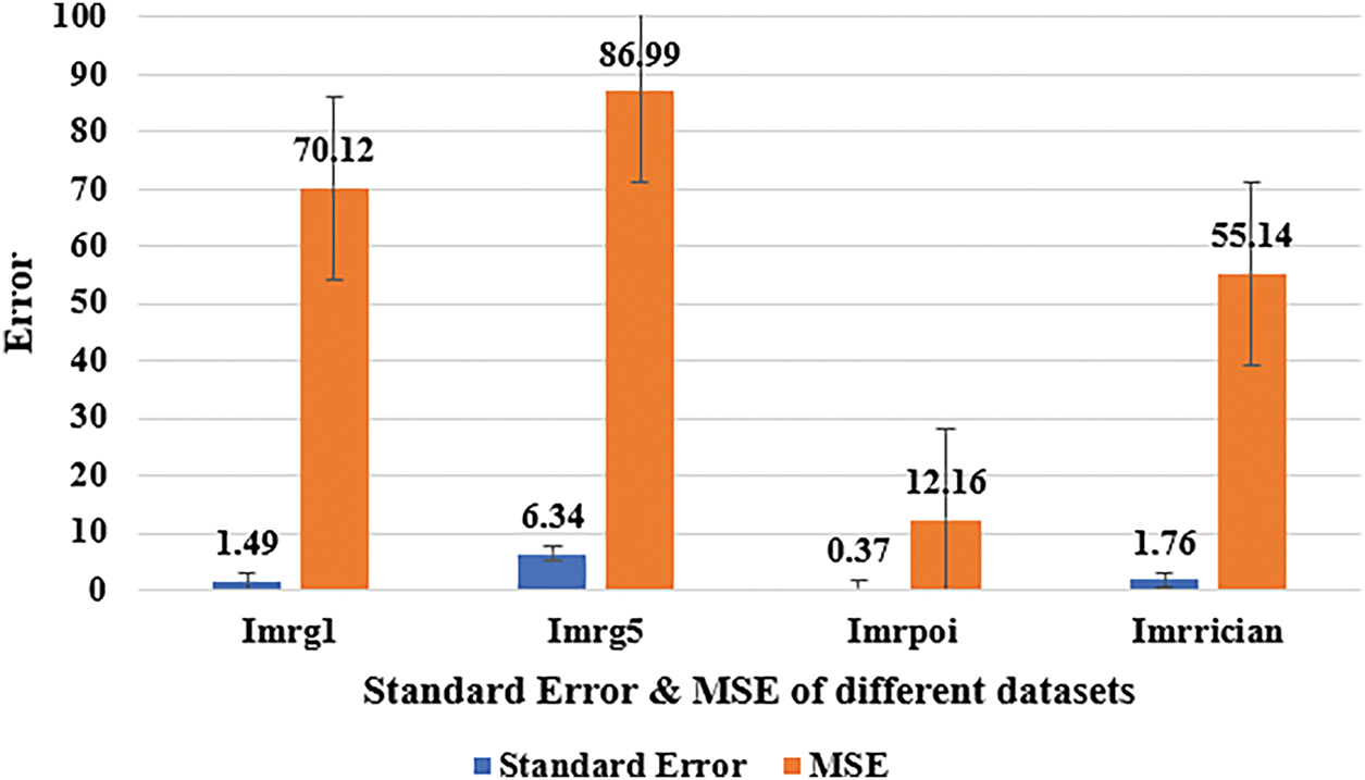
Figure 16: Standard error and MSE of different datasets
To support the points made above, the box plot for different parameters is shown in Fig. 17, (a) contrast, (b) correlation, (c) dissimilarity, (d) energy, (e) entropy, (f) MSE, (g) PSNR, (h) SSIM.
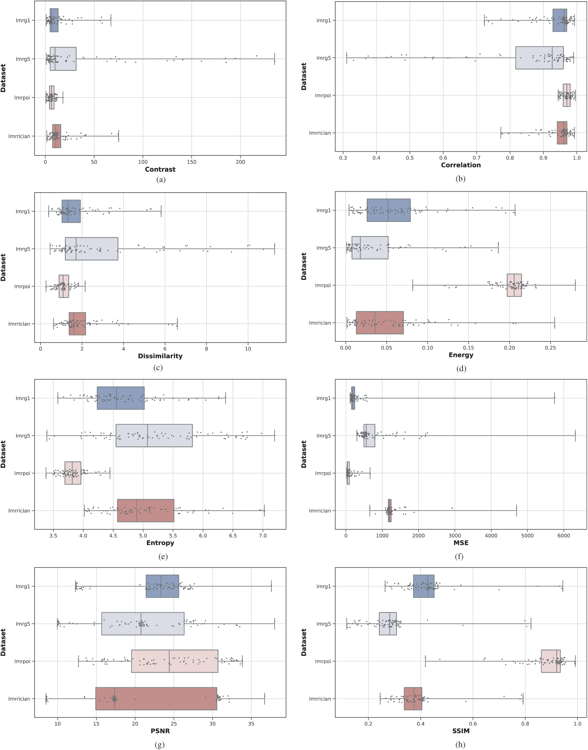
Figure 17: Boxplots for different metrics
Fig. 18 shows the correlation heatmaps that are used to depict the relation or to reveal the inter-dependency between the parameters for the four images (infected with noise) used in the denoising process.
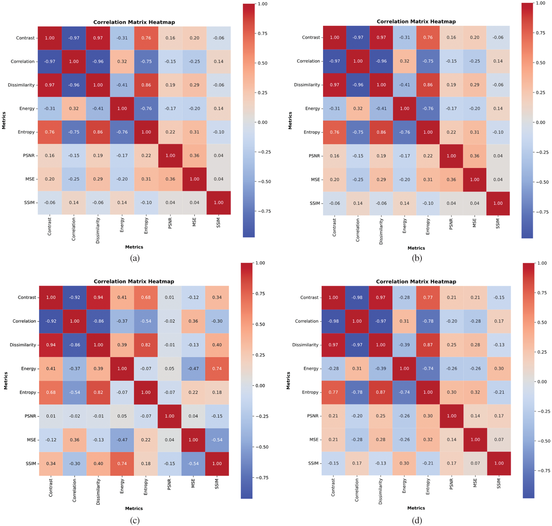
Figure 18: The correlation heatmaps for the parameters used for four different datasets
Table 19 illustrates the run time comparison of the current denoising methods. Total Variation (TV) and wavelet-based methods are some of the fastest due to their simpler implementation and lower computing complexity. Nevertheless, due to their complex model structures or redundant calculations, more sophisticated methods such as STROLLR and PCNN have greater processing times. Despite being designed over ten years ago, BM3D remains competitively fast and continues to be seen as a benchmark for speed and performance. On GPU platforms, the deep learning model DnCNN demonstrates high-speed inference; however, training these types of models continues to consume a lot of resources. This research enables practitioners and scholars to make more informed decisions by considering these runtime considerations.

While the principal interest of this research is the denoising ability of various strategies, it is equally important to consider the training time and computing demands of each method, especially when clinical integration is concerned, as time and resources are often limited. Although they exhibit poor denoising ability, spatial-domain filters are well-suited for real-time applications or emergencies because they require less processing power. Processing times for transform-based methods depend on the level of decomposition and the size of the transform kernel, leading to a significant increase in complexity, particularly during the decomposition and reconstruction processes. Even though dictionary learning and sparse-based methods yield great performance, they often require a huge amount of memory and long training times, especially when dealing with high-resolution 3D medical volumes. Depending on the optimization method and dictionary size, the training step can take hours. Deep learning-based techniques’ inference speed is typically fast after training, but preliminary training requires high-end GPUs and large annotated datasets, which may not always be feasible in low-resource clinical environments or in situations with time limitations. To better inform doctors and engineers regarding the suitability of techniques based on application constraints, future studies should standardly report training times, computation expenses, and hardware requirements.
The area of medical image denoising has undergone a sharp paradigm shift in recent times, owing to the revolutions in deep learning, where traditional rule-based approaches have been displaced by data-driven, end-to-end trainable models. One such innovation is the Denoising Convolutional Neural Network (DnCNN), which makes predictions and removes noise from medical images based on a deep residual learning architecture. When used in conjunction with batch normalization, its cascaded convolutional structure can learn complex noise patterns effectively without losing important structural features. This has performed effectively in medical environments to suppress modality-specific noise, for example, Poisson noise in low-dose CT or Rician noise in MRI. Also, newer techniques such as Content-Noise Complementary Learning (CNCL) enhance denoising performance while maintaining anatomical correctness through the utilization of dual neural predictors to separately learn noise and content in a complementary fashion. To produce perceptually realistic outputs, these models are often incorporated into generative adversarial network (GAN) pipelines. To search for optimal network architectures for specific denoising tasks, optimization methods such as genetic algorithms (GAs) have also been explored. These deep learning-founded models represent a significant advance beyond conventional filtering and transform-domain solutions with respect to generalization, flexibility, and modeling of noise.
Key Findings:
1. Best Feature Preservation
Deep learning-based methods, specifically DnCNN and CNCL, consistently preserve detailed anatomical and structural details with accuracy and effectively eliminate noise. Sparse representation methods also retain key features, making them ideal for clinical applications that require high fidelity.
2. Performance across Noise Types
Transform-based methods (e.g., wavelet, Shearlet) performed well on Gaussian and Poisson noise but performed poorly with Rician noise, typical in MRI. Some methods exhibited noise-type dependence, performing worse than their training and noise assumptions.
3. Image Orientation’s Effect
PSNR was significantly affected by a minor change in picture orientation or angle, highlighting the importance of evaluating resilience under collection conditions and data variability.
4. For measuring robustness, hybrid methods are best overall.
The most balanced results in terms of denoising power, structural retention, and noise variation flexibility were achieved by hybrid models that incorporate spatial, transform, and learning-based methods.
5. Accuracy and Efficiency Trade-off
Although deeper learning and sparse models require more training time and computing power, they achieve higher PSNR/SSIM. Although poor at preserving detailed information, spatial filters were nevertheless useful in low-resource or real-time situations.
6. The need for open, standard, and diverse datasets
The need for open, standard, and diverse datasets to ensure fair benchmarking and generalization is reinforced by the fluctuation of performance between methods.
8 Ethical, Regulatory, and Accountability Challenges in AI-Based Medical Image Denoising
AI-driven denoising of medical imaging, including MRI and CT scans, can make images clearer and more accurate for diagnosis, but it also raises important questions about ethics, regulations, and responsibility. We will go into more detail about these difficulties below, focusing on algorithmic bias, following medical device rules (FDA, CE, etc.), and the topic of who is responsible for automated diagnosis. We also talk about how contemporary trends in responsible AI and healthcare ethics are affecting these talks.
8.1 Ethical Concerns: Algorithmic Bias and Fairness in Denoising
• Algorithmic Bias in Medical Imaging: Deep learning models for image denoising can pick up and keep biases that are already in the data they were trained on. When talking about medical AI, “bias” means systemic mistakes that cause an algorithm’s predictions to be different from the truth, which could hurt some or all patients [357]. If a denoising algorithm is mostly trained on images from certain groups of people or scanner settings, it may not work as well for groups that are not well represented or for alternative equipment, which could lead to images of variable quality. These kinds of biases can harm patient outcomes by, for example, making minor indications of disease harder to detect or altering them in particular groups. In short, AI in medical imaging is at risk of different biases that could make diagnoses less accurate and make health inequities worse. A denoising model might “clean” what it believes is noise, but it could also eliminate or change clinically important features, like a faint tumor, by accident, especially if those features were infrequent or not present in the training data. This possibility is morally worrisome since it could cause some patients to be misdiagnosed or have their diagnosis delayed, which goes against the idea of justice (fair distribution of healthcare benefits).
• Fairness and Inclusivity: To be fair, the denoising method should make the images better for all patients in the same way. Bias might come from datasets that do not represent the whole population. For example, if an algorithm is trained largely on scans of younger adults, it might not work as well on older adults, or a model based on one hospital’s scanners might not work on other hospitals’ scanners. To fix this, the AI community stresses the importance of gathering a wide range of training data and doing in-depth subgroup studies to look for differences in performance between different groups of people. Bias auditing tools and fairness-aware algorithms that are meant to find and fix these kinds of problems are two examples of current responsible-AI trends. Finding and fixing AI bias before it causes problems later is really important. Researchers, for instance, say that denoising models should be tested on datasets from several centers and demographics, and that the models should be changed if any group displays worse performance. A worldwide evaluation also says that developers and radiologists need to be more conscious of bias and learn more about it. The paper says that increasing community understanding of bias (its sources, how to reduce it, and ethics) can lead to better regulatory frameworks and industry practices [357].
• Broader Ethical Principles: There are other ethical issues at stake besides bias. The World Health Organization (WHO) has set out six main rules for using AI in healthcare in an ethical way: (1) safeguard people’s freedom, (2) promote safety and health (and the public good), (3) make sure AI is clear and understandable, (4) encourage responsibility and accountability, (5) make sure everyone is included and treated fairly, and (6) encourage AI that is responsive and sustainable. These rules apply directly to algorithms that remove noise. For example, an AI denoiser should clearly benefit patient care (for example, by allowing lower radiation doses in CT) without adding new risks. Transparency means that the algorithm’s operation should be as clear as possible; for example, if a denoiser fails or changes an image, clinicians need to know how that happened. Patients should be told when AI is used in their imaging because of autonomy and informed consent. Right now, patients can sometimes choose not to have AI analysis, but this may not be possible if AI becomes more common. Privacy is another ethical issue because training and using these models generally needs a lot of patient scans, which raises problems regarding data privacy and consent. In the U.S, HIPAA and in Europe, GDPR protect patient data. Any AI method must follow these rules to be legal and ethical.
• Current Ethical Governance Trends: Bringing together AI and medical ethics has led to a lot of rules and frameworks. Professional groups, such as the RSNA and ACR in radiology, have written codes of ethics for AI that are based on the ideas of justice, beneficence, and openness. The World Health Organization’s standards (as indicated above) have become a standard for “responsible AI” in health around the world [Burac]. Another trend is the call for algorithmic transparency and explainability. This means making the “black box” AI easier to grasp so that doctors can trust the results and patients can trust them. Researchers are also looking into ways to measure how uncertain AI outputs are. This way, a denoising algorithm may tell when it is not sure about an image region instead of confidently changing it. To sum up, the ethical requirement is clear: AI image enhancement technologies must “promote well-being, minimize harm, and distribute benefits and harms fairly among all stakeholders.” This means that the technology should be fair, protect people’s privacy, and be overseen by people so that it helps everyone and does not make current inequities worse.
8.2 Regulatory Compliance: FDA, CE, and Global Oversight of AI Denoising
• Medical Device Regulations: Because the results of AI-driven image denoising tools used for diagnosis might affect clinical decisions, they are usually classified as medical devices, specifically as software as a medical device (SaMD). Before these instruments can be used on a large number of patients, regulatory bodies worldwide need proof that they are safe and effective. The FDA is in charge of AI/ML-based medical software in the US. If AI denoising algorithms are meant to change how a diagnosis is made, they are subject to FDA device review processes such as 510(k) clearances or De Novo authorization. The FDA has approved AI software that speeds up MRI scans by removing noise while keeping the quality of the images. This shows that the agency is willing to allow these kinds of tools if they are properly validated. The FDA usually wants strong clinical evidence that an AI-enhanced image is at least as good as a standard image for diagnosis. This means that studies need to show that radiologists can find problems just as well (or better) on denoised images as they can on regular images. Regulatory science is changing here: the FDA has said that the “traditional paradigm of device regulation was not designed for adaptive AI/ML technologies,” and many AI improvements could lead to new reviews under the current standards. The FDA then came out with an AI/ML Action Plan and guiding principles to change how they watch over learning algorithms. This involves promoting “Good Machine Learning Practice” and using tools like Predetermined Change Control Plans to make sure that AI models can update within set limits. Following FDA rules makes sure that an AI denoising tool has been thoroughly vetted for safety (it will not delete tumors or make artifacts) and effectiveness (it really does make images clearer or speed up diagnoses) [358].
The Medical Devices Regulation (MDR) says that AI-based medical image enhancers must get a CE mark in the European Union. The MDR (2017/745) says that most diagnostic software is at least Class IIa or higher-risk, which means that an independent notified body needs to look at it. Rule 11 of the MDR states that standalone software for diagnosis is typically considered to be at least Class IIa (moderate risk). To obtain CE certification, companies that develop denoising AI must adhere to strict guidelines for quality management, risk assessment, and clinical performance evidence. They must demonstrate that utilizing AI does not introduce any unacceptable risks, and in many cases, they must conduct clinical evaluations (reader studies or trials) to show that the diagnosis results are either better or the same. The EU AI Act, which will completely go into effect in 2026, will also create new rules for AI systems that are considered high-risk (most medical AI falls into this category). The AI Act says that high-risk AI, such as an automatic image analyzer, must employ “training, validation, and testing datasets that are relevant, representative, free of errors, and complete,” and put in place “bias monitoring and mitigation measures.” It also requires developers to be open with users and keep an eye on the product after it has been sold (for example, by keeping an eye on performance and reporting problems even after approval). This means that an AI denoising tool in the EU will need to undergo MDR’s device clearance process and comply with the AI Act’s rules on data and oversight to ensure it is safe, fair, and accountable.
• Global and Ongoing Regulatory Trends: Regulators all over the world are trying to figure out the best way to keep an eye on AI in healthcare. Many of them follow the same rules: a risk-based approach (more tight oversight for instruments that are more likely to cause problems), requiring proof of clinical validity, and making sure there are ways to control quality and keep an eye on things after they are deployed. The rules and regulations are always changing. For example, the FDA, the UK’s MHRA, Canada’s Health Canada, and others are working together to come up with common rules for AI-enabled devices. They do this through the International Medical Device Regulators Forum working groups. One interesting development is the provision of advice on systems for continuous learning. In the past, device approvals were set in stone; however, AI models can be learned from or modified. Regulators, such as the FDA, are exploring ways to facilitate safe upgrades without requiring approval each time. One way to do this is via a “predetermined change control plan,” which sets out and agrees on future model changes. Another tendency is that regulations are starting to include ethical AI standards. As was said before, the EU AI Act clearly includes requirements to deal with prejudice and openness. Regulators are increasingly starting to ask for documentation and openness in algorithms. For instance, producers might have to tell consumers (and regulators) how their model was trained, what its recognized limitations are, and how it was verified so that they know how to use it correctly. There is also a push for monitoring AI performance and negative occurrences in the actual world after deployment. The FDA’s action plan and others recommend gathering this kind of data. In general, compliance is not only a one-time checkbox; it is becoming an ongoing process (the “lifecycle” approach) where the AI must always be safe and useful in practice. In short, any deep learning denoising system that is meant to be used for automated diagnosis must go through a lot of complicated rules and get the required permissions (FDA clearance, CE mark, etc.) while also following new rules that make sure the system is reliable, reduces bias, and is open about how it works1,2,3.
8.3 Accountability in Automated Diagnosis and Image Enhancement
• Liability and Responsibility: “Who is responsible if something goes wrong?” with AI-assisted diagnostics is a big concern. Radiologists and doctors are in charge of looking at images and making diagnosis in today’s medical practice. If an AI-powered denoising or diagnostic recommendation leads to an error, such missing a malignancy or mistaking a normal structure for pathology, the guilt could fall on the doctor using the tool, the hospital that deployed it, or the software developer. Right now, there is not a clear legal agreement on who is responsible for AI in healthcare. There is not a “bright line” that separates the duties of healthcare providers, AI developers, and regulators.
Doctors can say that the AI made a bad recommendation and blame the manufacturer, while firms might say that the doctor is the one who makes the final decision. This lack of clarity makes it possible for there to be gaps in accountability, where a patient who is hurt by an AI mistake has trouble getting help since everyone is trying to avoid taking blame.
To fix this, experts and policymakers are asking for clear frameworks and comprehensive rules that make it obvious who is responsible. One approach is to treat AI diagnostic tools like human advisors. This means that a doctor must still follow the standard of care when using a tool. In real life, most regulators and professional guidelines still say that the human doctor is responsible for the diagnosis and that AI is just there to help. That is why most AI solutions are sold as “decision support” tools instead of technologies that make decisions on their own. But if AI gets better, this line may become less clear, and the law may need to change (for example, by creating rules for shared accountability or product liability for AI). The continuing international conversation around AI governance shows how important it is to find a balance between innovation and public safety. various countries have various levels of risk tolerance, but everyone agrees that without explicit responsibility, both patients and providers may lose faith in AI. New rules and standards are needed right now to make it clear who is responsible, protect patients, and make it clear how far the “AI supply chain” accountability goes from the data scientists who generated the model to the hospital that uses it3.
• Accountability Mechanisms and Oversight: In a larger sense, “accountability” involves putting rules and processes in place to make sure that AI systems are utilized properly and can be checked. One part is openness: if an AI denoising algorithm changes an image, it should keep a record of what it did and maybe even give a reason or a measure of uncertainty. It is difficult to hold people accountable when they cannot understand how black-box models work. As mentioned, AI systems that do not explain how they work make it harder to hold people accountable for judgments made by AI. As a way to hold AI developers accountable, the FDA and EU are pushing for transparency reports for AI technologies. Another thing is that people are in charge. Many ethicists support a “human-in-the-loop” paradigm, which says that AI can help but a qualified expert must check and can change the AI’s output, making sure that the AI is still responsible. In fact, the World Health Organization’s principle of accountability and many state guidelines say that humans, not only algorithms, should be responsible in the end. In reality, this means that radiology departments that use a denoising AI should have rules in place. For example, radiologists should know what the tool can and cannot do, there should be a mechanism to double-check AI results that do not make sense, and there should be a way to report AI problems.
• Legal and Ethical Developments: Some places are starting to deal with AI liability in the legal system. For instance, the EU AI Act will make it such that high-risk AI systems, like medical AI, have explicit ways to be held accountable. This will mean that makers have to keep an eye on how well the systems work and that users (hospitals) have to utilize them as they were meant to be used. Some people have said that the AI Act has “liability gaps” since it does not adequately explain who pays for damage produced by AI. People in the U.S. are still talking about whether the current laws on product liability and malpractice are good enough. If a denoising program that the FDA has cleared later turns out to create problems, patients might sue the company that made it for selling a bad product or the doctor for malpractice. The results may be different in each scenario. Some researchers suggest that AI mistakes should be covered via shared responsibility models or insurance plans. Professional indemnity insurers and hospital risk managers are looking into how AI use can change liability. Doctors are told to keep records of their use of AI and the reasons for it, just like they would for a consultation, to show that they did their due diligence.
• Building Accountability and Trust: To build trust in AI, stakeholders are putting in place mechanisms of responsibility that go beyond assigning blame. One important step is to keep an eye on and audit AI solutions once they are sold. Regulators and health organizations are thinking about making it necessary for AI tools to be tested in the real world all the time. For example, they could track diagnostic mistake rates before and after AI is used and have committees look into any significant accidents. As mentioned before, the EU AI Act will require continual monitoring of high-risk AI systems, and the FDA’s AI recommendations also stress the importance of evaluating how well AI works in the real world. Another way to promote accountability is to educate stakeholders, like doctors, about how the tool works and what it cannot accomplish. This makes it less likely that they will misuse it and more probable that they will find mistakes. Training for healthcare professionals on AI bias and how to utilize AI correctly is a common part of responsible AI projects in healthcare. Finally, traceability is important: AI systems should preserve precise records of their inputs, outputs, and model versions utilized so that if something goes wrong, it can be found and looked into. This is like an airplane’s “black box” for AI choices. It lets you look back and learn from mistakes and hold people accountable if necessary [357].
8.4 Trends in Responsible AI and Conclusion
The common thread running through all of these areas—ethics, regulation, and accountability—is the call for Responsible AI in healthcare. In the past few years, there has been a lot of work to make sure that AI tools like image denoisers are useful and safe. International organizations like the WHO and IEEE, as well as national agencies like the FDA’s AI program and the European Commission’s AI Act, are all working on guidelines that stress openness, fairness, and patient safety. For instance, the Who is principles sum up the idea of responsible AI, and the European Union’s AI Act is the first legal framework to define requirements for AI safety, openness, and reducing bias in high-risk areas like healthcare. The FDA is also releasing guiding principles and draft guidances for AI/ML-based medical devices. This shows that the agency is flexible in its approach to regulation, which fosters innovation while making sure that developers are responsible for the quality of their algorithms throughout the life cycle of the product [357].
To sum up, using deep learning to remove noise from MRI and CT images has clear benefits (faster scans, less radiation, cleaner images). Still, it must be done in a way that is ethical and follows the rules to avoid bias, make sure safety standards are met, and make sure everyone knows who is responsible. Some important considerations are ensuring that AI improvements benefit all patients equally by mitigating algorithmic bias, obtaining regulatory approval, and conducting thorough testing to demonstrate that denoising algorithms are both safe and effective. Another important consideration is ensuring patient safety when computerized systems are involved in their care, which can be achieved by maintaining accountability through transparency, oversight, and updated legal frameworks. The current trend in both business and government is toward “trustworthy AI,” which is AI that is accurate, easy to understand, fair, and properly governed. Developers and healthcare practitioners can utilize powerful denoising algorithms to enhance imaging and diagnosis without violating ethical guidelines or compromising patient trust, provided they adhere to new responsible-AI rules and practices. The primary goal is to utilize AI in a manner that enhances medical practice while adhering to the fundamental principles of medicine: do no harm, treat patients fairly, and ensure all clinical judgments are clear and accountable.
In conclusion, the domain of denoising methodologies for computed tomography (CT) and magnetic resonance imaging (MRI) images has undergone significant advancements throughout its history, driven by the imperative need to enhance image fidelity for precise diagnostic purposes and informed clinical judgments. Our comprehensive analysis of 80 denoising techniques elucidates the evolutionary trajectory from initial spatial-domain methodologies to sophisticated transform-based and data-driven approaches.
The preliminary phases of denoising predominantly relied on spatial-domain methodologies, wherein rudimentary filters were implemented to localize image regions. The methodologies above exhibited significant value due to their inherent simplicity and immediate applicability in real-time scenarios. However, their effectiveness was found to be constrained when confronted with intricate noise patterns and the imperative task of preserving intricate details. It is also evident that spatial filters are best suited for low-noise conditions. The guided image filter and Bitonic filter produced impressive results, but they were not entirely satisfactory.
With the advancement of the field, the emergence of transform-based methodologies heralded the onset of a new era. The utilization of Fourier domain and X-lets (Wavelets, Curvelets, Contourlets, Ridgelets, and shearlets) based denoising methodologies has effectively harnessed the computational capabilities of frequency decomposition, thereby facilitating the separation of noise components from the underlying signal. In the present context, these transforms have been extensively explored, and our review of these techniques concluded that the denoising performance improved with the evolution of these transforms, as they achieved more directionality and shift invariance. Although these methodologies exhibited enhanced noise reduction capabilities and the ability to maintain image structure, they frequently encountered challenges when dealing with complex noise patterns and non-stationary noise characteristics that are inherent in medical images. In addition, adopting a more effective shrinkage algorithm has always been a challenge.
The subsequent transition towards techniques based on sparsity denoted a paradigm shift of significant magnitude. Techniques such as sparse representation and dictionary learning have leveraged the innate sparsity present in medical images, thereby facilitating enhanced noise modeling and extraction capabilities. The methodologies as mentioned above demonstrated exceptional proficiency in capturing both global and local characteristics of images, rendering them highly suitable for preserving intricate anatomical structures and augmenting clinical interpretations.
The discernible effects resulting from the implementation of these disparate denoising paradigms are readily apparent. Spatial-domain methodologies, albeit constrained in their efficacy for mitigating noise, continue to be indispensable for expeditious applications and preliminary noise attenuation. The use of transform-based methodologies has led to notable improvements in noise reduction. However, the ability of these methods to effectively adapt to intricate noise patterns has proven to be a persistent challenge. Sparse-based methodologies, conversely, provide a synergistic amalgamation of noise mitigation and structure conservation, effectively catering to the distinct requirements of medical imaging, wherein intricate particulars assume paramount significance in the diagnostic process.
The lack of data diversity in most existing studies is a primary limitation. Precisely, fixed image orientations and limited noise models are commonly employed to measure denoising performance metrics such as PSNR. But in the real world, the medical images are taken from various angles and directions. The observations indicate that a small change in the image acquisition angle can lead to noticeable changes in PSNR values. This highlights that for a comprehensive evaluation of algorithmic performance, subsequent research needs to employ more diverse and representative datasets, considering variability in patient anatomy, scanner configurations, and acquisition angles.
As the domain advances, the symbiotic relationship between these denoising paradigms becomes progressively conspicuous. The utilization of hybrid methodologies that integrate spatial, transform, and sparse-based techniques demonstrates the inherent capacity to surmount the inherent constraints and shortcomings associated with each individual approach. Prospective investigations may be directed toward the utilization of deep learning methodologies to effectively integrate these paradigms, thereby establishing a cohesive structure that effectively leverages the synergistic capabilities of diverse techniques to achieve optimal noise mitigation and image enhancement.
In summary, the progressive advancement of denoising methodologies for computed tomography (CT) and magnetic resonance imaging (MRI) images signifies a trajectory from elementary approaches to intricate algorithms, emblematic of the unwavering dedication of the discipline to enhancing image fidelity and diagnostic precision. Given the ever-increasing intricacy of noise patterns observed in medical images, conventional denoising methods are facing significant challenges. However, the interaction between spatial, transform, and sparse-based techniques presents a highly promising direction for future research. This avenue holds great potential in the ongoing quest for noise-free medical images, which is crucial for the advancement of healthcare and medical imaging.
Acknowledgement: Not applicable.
Funding Statement: The authors received no specific funding for this study.
Author Contributions: Apoorav Sharma: Concept, Experimentation, Writing and Editing; Ayush Dogra: Experimentation and Writing; Bhawna Goyal: Validation and Visualization of Result; Archana Saini: Analysis of the Result and Proof Read; Vinay Kukreja: Formal Analysis of Result and Editing. All authors reviewed the results and approved the final version of the manuscript.
Availability of Data and Materials: The data that support the findings of this study are openly available at https://www.med.harvard.edu/AANLIB/.
Ethics Approval: No ethical approval needed.
Conflicts of Interest: The authors declare no conflicts of interest to report regarding the present study.
1https://www.fda.gov/downloads/medicaldevices/deviceregulationandguidance/guidancedocuments/ucm514737.pdf (accessed on 25 July 2025).
2http://www.fda.gov/cdrh/ode/guidance/1584.pdf (accessed on 25 July 2025).
3https://www.news-medical.net/health/Who-Takes-the-Blame-When-AI-Makes-a-Medical-Mistake.aspx (accessed on 25 July 2025).
References
1. Goyal B, Dogra A, Agrawal S, Sohi BS, Sharma A. Image denoising review: from classical to state-of-the-art approaches. Inf Fusion. 2020;55(2):220–44. doi:10.1016/j.inffus.2019.09.003. [Google Scholar] [CrossRef]
2. Mohd Sagheer SV, George SN. A review on medical image denoising algorithms. Biomed Signal Process Control. 2020;61(11):102036. doi:10.1016/j.bspc.2020.102036. [Google Scholar] [CrossRef]
3. Zhang X, Yan H. Medical image fusion and noise suppression with fractional-order total variation and multi-scale decomposition. IET Image Process. 2021;15(8):1688–701. doi:10.1049/ipr2.12137. [Google Scholar] [CrossRef]
4. Suganyadevi S, Seethalakshmi V, Balasamy K. A review on deep learning in medical image analysis. Int J Multim Inform Ret. 2022;11(1):19–38. doi:10.1007/s13735-021-00218-1. [Google Scholar] [PubMed] [CrossRef]
5. Patil R, Bhosale S. Medical image denoising techniques: a review. Int J Eng Sci Technol. 2022;4(1):21–33. doi:10.46328/ijonest.76. [Google Scholar] [CrossRef]
6. Tripti D, Mishra N, Khullar SS. Image denoising for medical image analysis. Int J Environ Sci. 2025;11(2s):1019–23. [Google Scholar]
7. Thanh D, Surya P, Hieu LM. A review on CT and X-ray images denoising methods. Informatica. 2019;43(2). doi:10.31449/inf.v43i2.2179. [Google Scholar] [CrossRef]
8. Ades-Aron B, Lemberskiy G, Veraart J, Golfinos J, Fieremans E, Novikov DS, et al. Improved task-based functional MRI language mapping in patients with brain tumors through marchenko-pastur principal component analysis denoising. Radiology. 2021;298(2):365–73. doi:10.1148/radiol.2020200822. [Google Scholar] [PubMed] [CrossRef]
9. Moore M, Iordan AD, Katsumi Y, Fabiani M, Gratton G, Dolcos F. Trimodal brain imaging: a novel approach for simultaneous investigation of human brain function. Biol Psychol. 2025;194(2):108967. doi:10.1016/j.biopsycho.2024.108967. [Google Scholar] [PubMed] [CrossRef]
10. Serai SD. Basics of magnetic resonance imaging and quantitative parameters T1, T2, T2*, T1rho and diffusion-weighted imaging. Pediatr Radiol. 2022;52(2):217–27. doi:10.1007/s00247-021-05042-7. [Google Scholar] [PubMed] [CrossRef]
11. Sullivan E, Thiruthaneeswaran N, Karpelowsky J, Busuttil G, Flower E, Bucci J, et al. The Australian paediatric brachytherapy experience: a pathway to a national programme. J Med Imag Rad Onc. 2024;1754–9485:13770. doi:10.1111/1754-9485.13770. [Google Scholar] [PubMed] [CrossRef]
12. Ryan S, McNicholas M, Eustace SJ. Anatomy for diagnostic imaging E-book: anatomy for diagnostic imaging E-book. The Netherlands: Elsevier Health Sciences; 2024. [Google Scholar]
13. Boukhennoufa N, Laamari Y, Benzid R. Signal denoising using a low computational translationin-variant- like strategy involving multiple wavelet bases: application to synthetic and ECG signals. Metrol Meas Syst. 2024;2024:259–78. doi:10.24425/mms.2024.148548. [Google Scholar] [CrossRef]
14. Xu W, Xiao C, Jia Z, Han Y. Digital image denoising method based on mean filter. In: 2020 International Conference on Computer Engineering and Application (ICCEA); 2020 Mar 18–20; Guangzhou, China: IEEE; 2020. p. 857–9. doi:10.1109/ICCEA50009.2020.00188. [Google Scholar] [CrossRef]
15. Thanh DNH, Engínoğlu S. An iterative mean filter for image denoising. IEEE Access. 2019;7:167847–59. doi:10.1109/access.2019.2953924. [Google Scholar] [CrossRef]
16. Gong Y, Liu B, Hou X, Qiu G. Sub-window box filter. In: 2018 IEEE Visual Communications and Image Processing (VCIP). Taichung, Taiwan; 2018. p. 1–4. doi:10.1109/vcip.2018.8698682. [Google Scholar] [CrossRef]
17. Shan X, Sun J, Guo Z, Yao W, Zhou Z. Fractional-order diffusion model for multiplicative noise removal in texture-rich images and its fast explicit diffusion solving. BIT Numer Math. 2022;62(4):1319–54. doi:10.1007/s10543-022-00913-3. [Google Scholar] [CrossRef]
18. Archana R, Eliahim Jeevaraj PS. Deep learning models for digital image processing: a review. Artif Intell Rev. 2024;57(1):11. doi:10.1007/s10462-023-10631-z. [Google Scholar] [CrossRef]
19. Taassori M, Vizvári B. Enhancing medical image denoising: a hybrid approach incorporating adaptive Kalman filter and non-local means with Latin square optimization. Electronics. 2024;13(13):2640. doi:10.3390/electronics13132640. [Google Scholar] [CrossRef]
20. AlRowaily MH, Arof H, Ibrahim I, Yazid H, Mahyiddin WA. Enhancing retina images by lowpass filtering using binomial filter. Diagnostics. 2024;14(15):1688. doi:10.3390/diagnostics14151688. [Google Scholar] [PubMed] [CrossRef]
21. Shangguan M, Yang Z, Lin Z, Weng Z, Sun J. Full-day profiling of a beam attenuation coefficient using a single-photon underwater lidar with a large dynamic measurement range. Opt Lett. 2024;49(3):626–9. doi:10.1364/OL.514622. [Google Scholar] [PubMed] [CrossRef]
22. Dhabal S, Chakrabarti R, Mishra NS, Venkateswaran P. An improved image denoising technique using differential evolution-based salp swarm algorithm. Soft Comput. 2021;25(3):1941–61. doi:10.1007/s00500-020-05267-y. [Google Scholar] [CrossRef]
23. Wang L, Jia H, Zhang Y, Li K, Wei C. EgpuIP: an embedded GPU accelerated library for image processing. In: 2022 IEEE 24th International Conference on High Performance Computing & Communications; 8th International Conference on Data Science & Systems; 20th International Conference on Smart City; 8th International Conference on Dependability in Sensor, Cloud & Big Data Systems & Application (HPCC/DSS/SmartCity/DependSys); 2022 Dec 18–20; Hainan, China: IEEE; 2022. p. 914–21. doi:10.1109/HPCC-DSS-SmartCity-DependSys57074.2022.00147. [Google Scholar] [CrossRef]
24. Bednar J, Watt T. Alpha-trimmed means and their relationship to Median filters. IEEE Trans Acoust Speech Signal Process. 1984;32(1):145–53. doi:10.1109/TASSP.1984.1164279. [Google Scholar] [CrossRef]
25. Khan KB, Amir M, Shahid M, Ullah H. Poisson noise reduction in scintigraphic images using Gradient Adaptive Trimmed Mean filter. In: 2016 International Conference on Intelligent Systems Engineering (ICISE); 2016 Jan 15–17; Islamabad, Pakistan: IEEE; 2016. p. 301–5. doi:10.1109/INTELSE.2016.7475138. [Google Scholar] [CrossRef]
26. Jana BR, Thotakura H, Baliyan A, Sankararao M, Deshmukh RG, Karanam SR. Pixel density based trimmed Median filter for removal of noise from surface image. Appl Nanosci. 2023;13(2):1017–28. doi:10.1007/s13204-021-01950-0. [Google Scholar] [CrossRef]
27. Harris FJ. Multirate signal processing for communication systems. Denmark: River Publishers; 2022. [Google Scholar]
28. Sabrine C, Abir S. Median filter for denoising MRI. Rev D’intelligence Artif. 2022;36(3):483–8. doi:10.18280/ria.360317. [Google Scholar] [CrossRef]
29. Yu J, Wei Y. Digital signal processing for high-speed THz communications. Chin J Electronics. 2022;31(3):534–46. doi:10.1049/cje.2021.00.258. [Google Scholar] [CrossRef]
30. Kumar A, Kumar S, Kar A. Salt and pepper denoising filters for digital images: a technical review. Serb J Electr Eng. 2024;21(3):429–66. doi:10.2298/sjee2403429k. [Google Scholar] [CrossRef]
31. Li X, Ji J, Li J, He S, Zhou Q. Research on image denoising based on Median filter. In: 2021 IEEE 4th Advanced Information Management, Communicates, Electronic and Automation Control Conference (IMCEC); 2021 Jun 18–20; Chongqing, China: IEEE; 2021. p. 528–31. doi:10.1109/IMCEC51613.2021.9482247. [Google Scholar] [CrossRef]
32. Ko SJ, Lee YH. Center weighted Median filters and their applications to image enhancement. IEEE Trans Circuits Syst. 1991;38(9):984–93. doi:10.1109/31.83870. [Google Scholar] [CrossRef]
33. Loupas T, McDicken WN, Allan PL. An adaptive weighted Median filter for speckle suppression in medical ultrasonic images. IEEE Trans Circuits Syst. 1989;36(1):129–35. doi:10.1109/31.16577. [Google Scholar] [CrossRef]
34. Oten R, de Figueiredo RJP. Adaptive alpha-trimmed mean filters under deviations from assumed noise model. IEEE Trans Image Process. 2004;13(5):627–39. doi:10.1109/tip.2003.821115. [Google Scholar] [PubMed] [CrossRef]
35. Peterson SR, Lee YH, Kassam SA. Some statistical properties of alpha-trimmed mean and standard type M filters. IEEE Trans Acoust Speech Signal Process. 1988;36(5):707–13. doi:10.1109/29.1580. [Google Scholar] [CrossRef]
36. Rahman MM, Abdullah-Al-Wadud M, Preza C. A decision-based filter for removing salt-and-pepper noise. In: 2012 International Conference on Informatics, Electronics & Vision (ICIEV); 2012 May 18–19; Dhaka, Bangladesh: IEEE; 2012. p. 1064–8. doi:10.1109/ICIEV.2012.6317513. [Google Scholar] [CrossRef]
37. Chalghoumi S, Smiti A. Median filter for denoising MRI: literature review. In: 2022 International Conference on Decision Aid Sciences and Applications (DASA); 2022 Mar 23–25; Chiangrai, Thailand: IEEE; 2022. p. 1603–6. doi:10.1109/DASA54658.2022.9764981. [Google Scholar] [CrossRef]
38. Toprak A, Güler İ. Impulse noise reduction in medical images with the use of switch mode fuzzy adaptive Median filter. Digit Signal Process. 2007;17(4):711–23. doi:10.1016/j.dsp.2006.11.008. [Google Scholar] [CrossRef]
39. Ghanekar U, Singh AK, Pandey R. A new scheme for impulse detection in switching Median filters for image filtering. In: International Conference on Computational Intelligence and Multimedia Applications (ICCIMA 2007); 2007 Dec 13–15; Sivakasi, India: IEEE; 2007. p. 442–6. doi:10.1109/ICCIMA.2007.284. [Google Scholar] [CrossRef]
40. Koli MA. Review of impulse noise reduction techniques. Int J Comput Sci Eng. 2012;4(2):184. [Google Scholar]
41. Sen AP, Rout NK. A comparative analysis of the algorithms for de-noising images contaminated with impulse noise. Sens Imag. 2022;23(1):11. doi:10.1007/s11220-022-00382-6. [Google Scholar] [CrossRef]
42. Omer AA, Hassan OI, Ahmed AI, Abdelrahman A. Denoising CT images using Median based filters: a review. In: 2018 International Conference on Computer, Control, Electrical, and Electronics Engineering (ICCCEEE); 2018 Aug 12–14; Khartoum, Sudan: IEEE; 2018. p. 1–6. doi:10.1109/ICCCEEE.2018.8515829. [Google Scholar] [CrossRef]
43. Ali HM. MRI medical image denoising by fundamental filters. In: High-resolution neuroimaging—basic physical principles and clinical applications. London, UK: InTech; 2018. doi:10.5772/intechopen.72427. [Google Scholar] [CrossRef]
44. Ning CY, Liu SF, Qu M. Research on removing noise in medical image based on Median filter method. In: 2009 IEEE International Symposium on IT in Medicine & Education; 2009 Aug 14–16; Jinan, China: IEEE; 2009. p. 384–8. doi:10.1109/ITIME.2009.5236393. [Google Scholar] [CrossRef]
45. Bhatia A. Salt-and-pepper noise elimination in medical image based on median filter method. Int J Electr Elect Data Commun. 2013 Aug;1(6):22–4. [Google Scholar]
46. Mohan J, Krishnaveni V, Guo Y. MRI denoising using nonlocal neutrosophic set approach of Wiener filtering. Biomed Signal Process Control. 2013;8(6):779–91. doi:10.1016/j.bspc.2013.07.005. [Google Scholar] [CrossRef]
47. Maneesha Mohan MR, Sulochana CH, Latha T. Medical image denoising using multistage directional Median filter. In: 2015 International Conference on Circuits, Power and Computing Technologies [ICCPCT-2015]; 2015 Mar 19–20; Nagercoil, India: IEEE; 2015. p. 1–6. doi:10.1109/ICCPCT.2015.7159261. [Google Scholar] [CrossRef]
48. Ye HJ, Zhang XY, He XG. Medical image denoising based on wavelet transform and median filtering. J Taiyuan Univ Technol. 2005;36(5):511–4. [Google Scholar]
49. Shreyamsha Kumar BK. Image denoising based on Gaussian/bilateral filter and its method noise thresholding. Signal Image Video Process. 2013;7(6):1159–72. doi:10.1007/s11760-012-0372-7. [Google Scholar] [CrossRef]
50. Kostková J, Flusser J, Lébl M, Pedone M. Handling Gaussian blur without deconvolution. Pattern Recognit. 2020;103(2):107264. doi:10.1016/j.patcog.2020.107264. [Google Scholar] [CrossRef]
51. Ito K, Xiong K. Gaussian filters for nonlinear filtering problems. IEEE Trans Autom Control. 2002;45(5):910–27. doi:10.1109/9.855552. [Google Scholar] [CrossRef]
52. Kumar GP. Analysis of visibility improvement based on Gaussian/bilateral filter. Int J Bioinform. 2022;1:5–8. [Google Scholar]
53. Pawar M, Sale D. MRI and CT image denoising using gaussian filter, wavelet transform and curvelet transform. Int J Eng Sci Comput. 2017 Jun;7(6):2321–3361. [Google Scholar]
54. Aubry M, Paris S, Hasinoff SW, Kautz J, Durand F. Fast local Laplacian filters. ACM Trans Graph. 2014;33(5):1–14. doi:10.1145/2629645. [Google Scholar] [CrossRef]
55. Paris S, Hasinoff SW, Kautz J. Local Laplacian filters: edge-aware image processing with a Laplacian pyramid. In: ACM SIGGRAPH 2011 papers. New York, NY, USA: ACM; 2011 Jul. p. 1–12. doi:10.1145/1964921.1964963. [Google Scholar] [CrossRef]
56. Du Z, Li X. Laplacian filtering effect on digital image tuning via the decomposed eigen-filter. Comput Electr Eng. 2019;78(5):69–78. doi:10.1016/j.compeleceng.2019.06.020. [Google Scholar] [CrossRef]
57. Song Y, Wu Y. An improved local Laplacian filter based on the relative total variation. Digit Signal Process. 2018;78(6):56–71. doi:10.1016/j.dsp.2018.02.004. [Google Scholar] [CrossRef]
58. Tomasi C, Manduchi R. Bilateral filtering for gray and color images. In: Sixth International Conference on Computer Vision; 1998 Jan 7; Bombay, India: IEEE; 1998. p. 839–46. doi:10.1109/ICCV.1998.710815. [Google Scholar] [CrossRef]
59. Patil PD, Kumbhar AD. Bilateral filter for image denoising. In: International Conference on Green Computing and Internet of Things (ICGCIoT); 2015 Oct 8–10; Greater Noida, India: IEEE; 2015. p. 299–302. doi:10.1109/ICGCIoT.2015.7380477. [Google Scholar] [CrossRef]
60. Wong WCK, Chung ACS, Yu SCH. Trilateral filtering for biomedical images. In: 2004 2nd IEEE International Symposium on Biomedical Imaging: Nano to Macro; 2004 Apr 18; Arlington, VA, USA: IEEE; 2004. p. 820–3. doi:10.1109/ISBI.2004.1398664. [Google Scholar] [CrossRef]
61. Ramkumar Raja M, Naveen R, Palaniswamy T, Mahendiran TV, Shukla NK, Verma R. A field programmable gate array-based biomedical noise reduction framework using advanced trilateral filter. Trans Inst Meas Control. 2021;43(16):3588–605. doi:10.1177/01423312211022200. [Google Scholar] [CrossRef]
62. Choudhury P, Tumblin J. The trilateral filter for high contrast images and meshes. In: SIGGRAPH '05: ACM SIGGRAPH 2005 Courses; 2005 Jul 31–Aug 4; Los Angeles, CA, USA: ACM; 2005. 5 p. doi:10.1145/1198555.1198565. [Google Scholar] [CrossRef]
63. Abid Ali AAM, Dohan MI, Musluh SK. Denoising of image using bilateral filtering in multiresolution. Csit. 2020;3(1):6–12. doi:10.34306/csit.v3i1.76. [Google Scholar] [CrossRef]
64. Zhang M, Gunturk BK. A new image denoising framework based on bilateral filter. In: Visual communications and image processing 2008. San Jose, CA, USA: SPIE; 2008. doi:10.1117/12.768101. [Google Scholar] [CrossRef]
65. Shanthi SA, Sulochana CH, Jerome SA. Image denoising using bilateral filter in subsampled pyramid and nonsubsampled directional filter bank domain. J Intell Fuzzy Syst. 2016;31(1):237–47. doi:10.3233/ifs-162137. [Google Scholar] [CrossRef]
66. Vinodhbabu P, Swapna P. A new method for medical image denoising using DTCWT and bilateral filter. Int J Innov Technol Explor Eng. 2019;8(12):2925–30. doi:10.35940/ijitee.k1882.1081219. [Google Scholar] [CrossRef]
67. Thakur K, Damodare O, Sapkal A. Hybrid method for medical image denoising using Shearlet transform and bilateral filter. In: 2015 International Conference on Information Processing (ICIP); 2015 Dec 16–19; Pune, India: IEEE; 2015. p. 220–4. doi:10.1109/INFOP.2015.7489382. [Google Scholar] [CrossRef]
68. Wang T, Feng H, Li S, Yang Y. Medical image denoising using bilateral filter and the K-SVD algorithm. J Phys Conf Ser. 2019;1229(1):012007. doi:10.1088/1742-6596/1229/1/012007. [Google Scholar] [CrossRef]
69. Elhoseny M, Shankar K. Optimal bilateral filter and Convolutional Neural Network based denoising method of medical image measurements. Measurement. 2019;143(9):125–35. doi:10.1016/j.measurement.2019.04.072. [Google Scholar] [CrossRef]
70. Joseph J, Periyasamy R. An image driven bilateral filter with adaptive range and spatial parameters for denoising Magnetic Resonance Images. Comput Electr Eng. 2018;69:782–95. doi:10.1016/j.compeleceng.2018.02.033. [Google Scholar] [CrossRef]
71. Singh RP, Varma V, Chaudhary P. A hybrid technique for medical image denoising using neural network, bilateral filter and LDA. Int J Fuzzy Reason Soft Comput. 2012;1(1):1–5. [Google Scholar]
72. Liang GS, Wang RW, Wen XB. Image denoising based on bilateral filtering and non-local means. J Phy Conf Ser. 2014;559(1):012088. [Google Scholar]
73. Caraffa L, Tarel JP, Charbonnier P. The guided bilateral filter: when the joint/cross bilateral filter becomes robust. IEEE Trans Image Process. 2015;24(4):1199–208. doi:10.1109/tip.2015.2389617. [Google Scholar] [PubMed] [CrossRef]
74. He K, Sun J, Tang X. Guided image filtering. IEEE Trans Pattern Anal Mach Intell. 2013;35(6):1397–409. doi:10.1109/tpami.2012.213. [Google Scholar] [PubMed] [CrossRef]
75. He K, Sun J. Fast guided filter. In: Proceedings of 14th European Conference on Computer Vision (ECCV). Amsterdam, The Netherlands; 2016 Oct. p. 717–32. doi:10.1007/978-3-319-46487-9_44. [Google Scholar] [CrossRef]
76. Ochotorena CN, Yamashita Y. Anisotropic guided filtering. IEEE Trans Image Process. 2019;29:1397–412. doi:10.1109/TIP.2019.2941326. [Google Scholar] [PubMed] [CrossRef]
77. Yin H, Gong Y, Qiu G. Side window guided filtering. Signal Process. 2019;165(11):315–30. doi:10.1016/j.sigpro.2019.07.026. [Google Scholar] [CrossRef]
78. Wu H, Zheng S, Zhang J, Huang K. Fast end-to-end trainable guided filter. In: 2018 IEEE/CVF Conference on Computer Vision and Pattern Recognition; 2018 Jun 18–23; Salt Lake City, UT, USA: IEEE; 2018. p. 1838–47. doi:10.1109/CVPR.2018.00197. [Google Scholar] [CrossRef]
79. Kou F, Chen W, Wen C, Li Z. Gradient domain guided image filtering. IEEE Trans Image Process. 2015;24(11):4528–39. doi:10.1109/TIP.2015.2468183. [Google Scholar] [PubMed] [CrossRef]
80. Qiu Y, Urahama K. Denoising of multi-modal images with PCA self-cross bilateral filter. IEICE Trans Fundamentals. 2010;E93-A(9):1709–12. doi:10.1587/transfun.e93.a.1709. [Google Scholar] [CrossRef]
81. Majeeth SS, Babu CNK. Gaussian noise removal in an image using fast guided filter and its method noise thresholding in medical healthcare application. J Med Syst. 2019;43(8):280. doi:10.1007/s10916-019-1376-4. [Google Scholar] [PubMed] [CrossRef]
82. Chun SY. Iterative guided image filtering for multimodal medical imaging. In: 2015 IEEE Nuclear Science Symposium and Medical Imaging Conference (NSS/MIC); 2015 Oct 31–Nov 7; San Diego, CA, USA: IEEE; 2015. p. 1–4. doi:10.1109/NSSMIC.2015.7582232. [Google Scholar] [CrossRef]
83. Gautam D, Khare K, Shrivastava BP. A novel guided box filter based on hybrid optimization for medical image denoising. Appl Sci. 2023;13(12):7032. doi:10.3390/app13127032. [Google Scholar] [CrossRef]
84. Robbins GM, Huang TS. Inverse filtering for linear shift-variant imaging systems. Proc IEEE. 1972;60(7):862–72. doi:10.1109/PROC.1972.8785. [Google Scholar] [CrossRef]
85. Michailovich O, Tannenbaum A. Blind deconvolution of medical ultrasound images: a parametric inverse filtering approach. IEEE Trans Image Process. 2007;16(12):3005–19. doi:10.1109/TIP.2007.910179. [Google Scholar] [PubMed] [CrossRef]
86. Haddadi YR, Mansouri B, Khodja FZD. A novel bio-inspired optimization algorithm for medical image restoration using Enhanced Regularized Inverse Filtering. Res Biomed Eng. 2023;39(1):233–44. doi:10.1007/s42600-023-00269-9. [Google Scholar] [CrossRef]
87. Jacob NA, Martin A. Image denoising in the wavelet domain using Wiener filtering, In: Project report. Madison, WI, USA: University of Wisconsin; 2004 Dec. [Google Scholar]
88. Zhang X. Image denoising using local Wiener filter and its method noise. Optik. 2016;127(17):6821–8. doi:10.1016/j.ijleo.2016.05.002. [Google Scholar] [CrossRef]
89. Zhang H, Nosratinia A, Wells RO. Image denoising via wavelet-domain spatially adaptive FIR Wiener filtering. In: 2000 IEEE International Conference on Acoustics, Speech, and Signal Processing. Proceedings (Cat. No.00CH37100); 2000 Jun 5–9; Istanbul, Turkey: IEEE; 2000 Aug. p. 2179–82. doi:10.1109/ICASSP.2000.859269. [Google Scholar] [CrossRef]
90. Wang Z, Qu C, Cui L. Denoising images using Wiener filter in directionalet domain. In: 2006 International Conference on Computational Inteligence for Modelling Control and Automation and International Conference on Intelligent Agents Web Technologies and International Commerce (CIMCA’06); 2006 Nov 28–Dec 1; Sydney, NSW, Australia: IEEE; 2006. doi:10.1109/CIMCA.2006.80. [Google Scholar] [CrossRef]
91. Mohan J, Guo Y, Krishnaveni V, Jeganathan K. MRI denoising based on neutrosophic Wiener filtering. In: 2012 IEEE International Conference on Imaging Systems and Techniques Proceedings; 2012 Jul 16–17; Manchester, UK: IEEE; 2012. p. 327–31. doi:10.1109/IST.2012.6295518. [Google Scholar] [CrossRef]
92. Wang L, Zou YK, Zhang HJ. A medical image denoising arithmetic based on Wiener filter parallel model of wavelet transform. In: 2009 2nd International Congress on Image and Signal Processing; 2009 Oct 17–19; Tianjin, China: IEEE; 2009. p. 1–4. doi:10.1109/CISP.2009.5304080. [Google Scholar] [CrossRef]
93. Naimi H, Adamou-Mitiche ABH, Mitiche L. Medical image denoising using dual tree complex thresholding wavelet transform and Wiener filter. J King Saud Univ Comput Inf Sci. 2015;27(1):40–5. doi:10.1016/j.jksuci.2014.03.015. [Google Scholar] [CrossRef]
94. Tayade PM, Bhosale SP. Medical image denoising and enhancement using DTCWT and Wiener filter. Inte J Adv Res, Ideas Innovat Technol. 2018;4(4):342–44. [Google Scholar]
95. Kazubek M. Wavelet domain image denoising by thresholding and Wiener filtering. IEEE Signal Process Lett. 2003;10(11):324–6. doi:10.1109/LSP.2003.818225. [Google Scholar] [CrossRef]
96. Lahmiri S. An iterative denoising system based on Wiener filtering with application to biomedical images. Opt Laser Technol. 2017;90:128–32. doi:10.1016/j.optlastec.2016.11.015. [Google Scholar] [CrossRef]
97. Bapat A, Frahm JM. The domain transform solver. In: 2019 IEEE/CVF Conference on Computer Vision and Pattern Recognition (CVPR); 2019 Jun 15–20; Long Beach, CA, USA: IEEE; 2019. p. 6007–16. doi:10.1109/cvpr.2019.00617. [Google Scholar] [CrossRef]
98. Gastal ESL, Oliveira MM. Domain transform for edge-aware image and video processing. In: SIGGRAPH '11: ACM SIGGRAPH 2011 Papers. Vancouver, BC, Canada: ACM; 2011. p. 1–12. doi:10.1145/1964921.1964964. [Google Scholar] [CrossRef]
99. Goyal B, Chyophel Lepcha D, Dogra A, Bhateja V, Lay-Ekuakille A. Measurement and analysis of multi-modal image fusion metrics based on structure awareness using domain transform filtering. Measurement. 2021;182(8):109663. doi:10.1016/j.measurement.2021.109663. [Google Scholar] [CrossRef]
100. He L, Schaefer S. Mesh denoising via L0 minimization. ACM Trans Graph. 2013;32(4):1–8. doi:10.1145/2461912.2461965. [Google Scholar] [CrossRef]
101. Selvin S, Ajay SG, Gowri BG, Sowmya V, Soman KP. ℓ1 trend filter for image denoising. Procedia Comput Sci. 2016;93(2):495–502. doi:10.1016/j.procs.2016.07.239. [Google Scholar] [CrossRef]
102. Thanh DNH, Thanh LT, Hien NN, Prasath S. Adaptive total variation L1 regularization for salt and pepper image denoising. Optik. 2020;208(5):163677. doi:10.1016/j.ijleo.2019.163677. [Google Scholar] [CrossRef]
103. Łasica M, Moll S, Mucha PB. Total variation denoising in l1 anisotropy. SIAM J Imaging Sci. 2017;10(4):1691–723. doi:10.1137/16m1103610. [Google Scholar] [CrossRef]
104. Verma M, Raman B, Murala S. Local extrema co-occurrence pattern for color and texture image retrieval. Neurocomputing. 2015;165(5):255–69. doi:10.1016/j.neucom.2015.03.015. [Google Scholar] [CrossRef]
105. Shi K, Liu A, Zhang J, Liu Y, Chen X. Medical image fusion based on multilevel bidirectional feature interaction network. IEEE Sens J. 2024;24(12):19428–41. doi:10.1109/JSEN.2024.3393619. [Google Scholar] [CrossRef]
106. Goyal B, Lepcha DC, Dogra A, Wang SH. A weighted least squares optimisation strategy for medical image super resolution via multiscale convolutional neural networks for healthcare applications. Complex Intell Syst. 2022;8(4):3089–104. doi:10.1007/s40747-021-00465-z. [Google Scholar] [CrossRef]
107. Luo J, Li J, Wang X, Feng S. An inductive sensor based multi-least-mean-square adaptive weighting filtering for debris feature extraction. IEEE Trans Ind Electron. 2023;70(3):3115–25. doi:10.1109/TIE.2022.3169720. [Google Scholar] [CrossRef]
108. Wang Z, Na Y, Liu Z, Tian B, Fu Q. Weighted recursive least square filter and neural network based residual ECHO suppression for the AEC-challenge. In: ICASSP 2021-2021 IEEE International Conference on Acoustics, Speech and Signal Processing (ICASSP); 2021 Jun 6–11; Toronto, ON, Canada: IEEE; 2021. p. 141–5. doi:10.1109/ICASSP39728.2021.9414623. [Google Scholar] [CrossRef]
109. Wang J, Li T, Lu H, Liang Z. Penalized weighted least-squares approach to sinogram noise reduction and image reconstruction for low-dose X-ray computed tomography. IEEE Trans Med Imaging. 2006;25(10):1272–83. doi:10.1109/42.896783. [Google Scholar] [CrossRef]
110. Jiang W, Yang X, Wu W, Liu K, Ahmad A, Sangaiah AK, et al. Medical images fusion by using weighted least squares filter and sparse representation. Comput Electr Eng. 2018;67(3):252–66. doi:10.1016/j.compeleceng.2018.03.037. [Google Scholar] [CrossRef]
111. Gong S, Li S, Zhang Z, Xia M. Nonlinear blind deconvolution based on generalized normalized lp/lq norm for early fault detection. IEEE Trans Instrum Meas. 2024;73:3507512. doi:10.1109/TIM.2023.3346518. [Google Scholar] [CrossRef]
112. Zhu XH, Li MT, Deng YJ, Luo X, Shen LM, Long CF. L2, 1-norm regularized double non-negative matrix factorization for hyperspectral change detection. Symmetry. 2025;17(2):304. doi:10.3390/sym17020304. [Google Scholar] [CrossRef]
113. Yue L, Shen H, Yuan Q, Zhang L. A locally adaptive L1−L2 norm for multi-frame super-resolution of images with mixed noise and outliers. Signal Process. 2014;105(3):156–74. doi:10.1016/j.sigpro.2014.04.031. [Google Scholar] [CrossRef]
114. Haji SH, Abdulazeez AM. Comparison of optimization techniques based on gradient descent algorithm: a review. PalArch’s J Archaeol Egypt/Egyptol. 2021;18(4):2715–43. [Google Scholar]
115. Bottou L. Stochastic gradient descent tricks. In: Neural networks: tricks of the trade. Berlin/Heidelberg: Springer; 2012. p. 421–36. doi:10.1007/978-3-642-35289-8_25. [Google Scholar] [CrossRef]
116. Ben-Loghfyry A, Hakim A, Laghrib A. A denoising model based on the fractional Beltrami regularization and its numerical solution. J Appl Math Comput. 2023;69(2):1431–63. doi:10.1007/s12190-022-01798-9. [Google Scholar] [CrossRef]
117. Consonni G, Veronese P. Conjugate priors for exponential families having quadratic variance functions. J Am Stat Assoc. 1992;87(420):1123–7. doi:10.1080/01621459.1992.10476268. [Google Scholar] [CrossRef]
118. Mehranian A, Belzunce MA, McGinnity CJ, Bustin A, Prieto C, Hammers A, et al. Multi-modal synergistic PET and MR reconstruction using mutually weighted quadratic priors. Magn Reson Med. 2019;81(3):2120–34. doi:10.1002/mrm.27521. [Google Scholar] [PubMed] [CrossRef]
119. Zadorozhnyi O, Benecke G, Mandt S, Scheffer T, Kloft M. Huber-norm regularization for linear prediction models. In: Machine learning and knowledge discovery in databases. Cham: Springer International Publishing; 2016. p. 714–30. doi:10.1007/978-3-319-46128-1_45. [Google Scholar] [CrossRef]
120. Prudhvi Raj VN. Denoising of medical images using total variational method. Signal Image Process. 2012;3(2):131–42. doi:10.5121/sipij.2012.3209. [Google Scholar] [CrossRef]
121. Diwakar M, Kumar P, Singh P, Tripathi A, Singh L. An efficient reversible data hiding using SVD over a novel weighted iterative anisotropic total variation based denoised medical images. Biomed Signal Process Control. 2023;82(1):104563. doi:10.1016/j.bspc.2022.104563. [Google Scholar] [CrossRef]
122. Laves MH, Tölle M, Ortmaier T. Uncertainty estimation in medical image denoising with Bayesian deep image prior. In: Uncertainty for safe utilization of machine learning in medical imaging, and graphs in biomedical image analysis. Cham: Springer International Publishing; 2020. p. 81–96. doi:10.1007/978-3-030-60365-6_9. [Google Scholar] [CrossRef]
123. Ben Said A, Hadjidj R, Foufou S. Total variation for image denoising based on a novel smart edge detector: an application to medical images. J Math Imag Vis. 2019;61(1):106–21. doi:10.1007/s10851-018-0829-6. [Google Scholar] [CrossRef]
124. Rudin LI, Osher S, Fatemi E. Nonlinear total variation based noise removal algorithms. Phys D Nonlinear Phenom. 1992;60(1–4):259–68. doi:10.1016/0167-2789(92)90242-F. [Google Scholar] [CrossRef]
125. Jevnisek RJ, Avidan S. Co-occurrence filter. In: 2017 IEEE Conference on Computer Vision and Pattern Recognition (CVPR); 2017 Jul 21–26; Honolulu, HI, USA: IEEE; 2017. p. 3816–24. doi:10.1109/CVPR.2017.406. [Google Scholar] [CrossRef]
126. Sun Z, Liu T, Li J, Wang Y, Gao X. Patch-based co-occurrence filter with fast adaptive kernel. Signal Process. 2021;185(7):108089. doi:10.1016/j.sigpro.2021.108089. [Google Scholar] [CrossRef]
127. Jon K, Liu J, Lv X, Zhu W. Poisson noisy image restoration via overlapping group sparse and nonconvex second-order total variation priors. PLoS One. 2021;16(4):e0250260. doi:10.1371/journal.pone.0250260. [Google Scholar] [PubMed] [CrossRef]
128. Chambolle A. An algorithm for total variation minimization and applications. J Math Imag Vis. 2004;20(1):89–97. doi:10.1023/B:JMIV.0000011325.36760.1e. [Google Scholar] [CrossRef]
129. Li B, Que D. Medical images denoising based on total variation algorithm. Procedia Environ Sci. 2011;8:227–34. doi:10.1016/j.proenv.2011.10.037. [Google Scholar] [CrossRef]
130. Easley GR, Labate D, Colonna F. Shearlet-based total variation diffusion for denoising. IEEE Trans Image Process. 2008;18(2):260–8. doi:10.1109/TIP.2008.2008070. [Google Scholar] [PubMed] [CrossRef]
131. Dai S. Variable selection in convex quantile regression: L1-norm or L0-norm regularization? Eur J Oper Res. 2023;305(1):338–55. doi:10.1016/j.ejor.2022.05.041. [Google Scholar] [CrossRef]
132. Hyder M, Mahata K. An approximate L0 norm minimization algorithm for compressed sensing. In: 2009 IEEE International Conference on Acoustics, Speech and Signal Processing; 2009 Apr 19–24; Taipei, Taiwan: IEEE; 2009. p. 3365–8. doi:10.1109/ICASSP.2009.4960346. [Google Scholar] [CrossRef]
133. Mancera L, Portilla J. L0-norm-based sparse representation through alternate projections. In: 2006 International Conference on Image Processing; 2006 Oct 8–11; Atlanta, GA, USA: IEEE; 2006. p. 2089–92. doi:10.1109/ICIP.2006.312819. [Google Scholar] [CrossRef]
134. Micchelli CA, Shen L, Xu Y, Zeng X. Proximity algorithms for the L1/TV image denoising model. Adv Comput Math. 2013;38(2):401–26. doi:10.1007/s10444-011-9243-y. [Google Scholar] [CrossRef]
135. Sun Y, Schaefer S, Wang W. Denoising point sets via L0 minimization. Comput Aided Geom Des. 2015;35-36(1):2–15. doi:10.1016/j.cagd.2015.03.011. [Google Scholar] [CrossRef]
136. Bai F, Franchois A, Pizurica A. 3d microwave tomography with Huber regularization applied to realistic numerical breast phantoms. Prog Electromagn Res. 2016;155:75–91. doi:10.2528/pier15121703. [Google Scholar] [CrossRef]
137. Odille F, Bustin A, Chen B, Vuissoz PA, Felblinger J. Motion-corrected, super-resolution reconstruction for high-resolution 3D cardiac cine MRI. In: Medical image computing and computer-assisted intervention–MICCAI 2015. Cham: Springer International Publishing; 2015. p. 435–42. doi:10.1007/978-3-319-24574-4_52. [Google Scholar] [CrossRef]
138. Muneeswaran V, Pallikonda Rajasekaran M. Beltrami-regularized denoising filter based on tree seed optimization algorithm: an ultrasound image application. In: Information and communication technology for intelligent systems (ICTIS 2017). Vol. 1. Cham: Springer International Publishing; 2017. p. 449–57. doi:10.1007/978-3-319-63673-3_54. [Google Scholar] [CrossRef]
139. Blei DM, Kucukelbir A, McAuliffe JD. Variational inference: a review for statisticians. J Am Stat Assoc. 2017;112(518):859–77. doi:10.1080/01621459.2017.1285773. [Google Scholar] [CrossRef]
140. Lorenz D, Worliczek N. Necessary conditions for variational regularization schemes. Inverse Probl. 2013;29(7):075016. doi:10.1088/0266-5611/29/7/075016. [Google Scholar] [CrossRef]
141. Lahmiri S, Boukadoum M. Biomedical image denoising using variational mode decomposition. In: 2014 IEEE Biomedical Circuits and Systems Conference (BioCAS) Proceedings; 2014 Oct 22–24; Lausanne, Switzerland: IEEE; 2014. p. 340–3. doi:10.1109/BioCAS.2014.6981732. [Google Scholar] [CrossRef]
142. Rapisarda E, Presotto L, De Bernardi E, Gilardi MC, Bettinardi V. Optimized Bayes variational regularization prior for 3D PET images. Comput Med Imaging Graph. 2014;38(6):445–57. doi:10.1016/j.compmedimag.2014.05.004. [Google Scholar] [PubMed] [CrossRef]
143. Le T, Chartrand R, Asaki TJ. A variational approach to reconstructing images corrupted by Poisson noise. J Math Imag Vis. 2007;27(3):257–63. doi:10.1007/s10851-007-0652-y. [Google Scholar] [CrossRef]
144. Li F, Abascal JFPJ, Desco M, Soleimani M. Total variation regularization with split bregman-based method in magnetic induction tomography using experimental data. IEEE Sens J. 2016;17(4):976–85. doi:10.1109/JSEN.2016.2637411. [Google Scholar] [CrossRef]
145. Li W, Li Q, Gong W, Tang S. Total variation blind deconvolution employing split Bregman iteration. J Vis Commun Image Represent. 2012;23(3):409–17. doi:10.1016/j.jvcir.2011.12.003. [Google Scholar] [CrossRef]
146. Kervrann C, Boulanger J. Unsupervised patch-based image regularization and representation. In: Computer vision–ECCV 2006. Berlin/Heidelberg, Germany: Springer; 2006. p. 555–67. doi:10.1007/11744085_43. [Google Scholar] [CrossRef]
147. Gilton D, Ongie G, Willett R. Learned patch-based regularization for inverse problems in imaging. In: 2019 IEEE 8th International Workshop on Computational Advances in Multi-Sensor Adaptive Processing (CAMSAP); 2019 Dec 15–18; Le gosier, Guadeloupe: IEEE; 2019. p. 211–5. doi:10.1109/camsap45676.2019.9022624. [Google Scholar] [CrossRef]
148. Jain P, Tyagi V. LAPB: locally adaptive patch-based wavelet domain edge-preserving image denoising. Inf Sci. 2015;294(455):164–81. doi:10.1016/j.ins.2014.09.060. [Google Scholar] [CrossRef]
149. Wang G, Qi J. Penalized likelihood PET image reconstruction using patch-based edge-preserving regularization. IEEE Trans Med Imaging. 2012;31(12):2194–204. doi:10.1109/tmi.2012.2211378. [Google Scholar] [PubMed] [CrossRef]
150. Feng J, Song L, Huo X, Yang X, Zhang W. An optimized pixel-wise weighting approach for patch-based image denoising. IEEE Signal Process Lett. 2015;22(1):115–9. doi:10.1109/LSP.2014.2350032. [Google Scholar] [CrossRef]
151. Jiang B, Lu Y, Zhang B, Lu G. AGP-net: adaptive graph prior network for image denoising. IEEE Trans Ind Inform. 2024;20(3):4753–64. doi:10.1109/TII.2023.3316184. [Google Scholar] [CrossRef]
152. Malfait M, Roose D. Wavelet-based image denoising using a Markov random field a priori model. IEEE Trans Image Process. 1997;6(4):549–65. doi:10.1109/83.563320. [Google Scholar] [PubMed] [CrossRef]
153. Zhu SC, Mumford D. Prior learning and Gibbs reaction-diffusion. IEEE Trans Pattern Anal Mach Intell. 1997;19(11):1236–50. doi:10.1109/34.632983. [Google Scholar] [CrossRef]
154. Sulam J, Elad M. Expected patch log likelihood with a sparse prior. In: International Workshop on Energy Minimization Methods in Computer Vision and Pattern Recognition. Cham: Springer International Publishing; 2015. p. 99–111. doi:10.1007/978-3-319-14612-6_8. [Google Scholar] [CrossRef]
155. Tian C, Fei L, Zheng W, Xu Y, Zuo W, Lin CW. Deep learning on image denoising: an overview. Neural Netw. 2020;131(11):251–75. doi:10.1016/j.neunet.2020.07.025. [Google Scholar] [PubMed] [CrossRef]
156. Xie J, Xu L, Chen E. Image denoising and inpainting with deep neural networks. Adv Neural Inform Process Syst. 2012;25:1–9. [Google Scholar]
157. Rai S, Bhatt JS, Patra SK. An unsupervised deep learning framework for medical image denoising. arXiv:2103.06575. 2021. doi:10.48550/arXiv.2103.06575. [Google Scholar] [CrossRef]
158. Wang Z, Wang L, Duan S, Li Y. An image denoising method based on deep residual GAN. J Phys Conf Ser. 2020;1550(3):032127. doi:10.1088/1742-6596/1550/3/032127. [Google Scholar] [CrossRef]
159. Haralick RM, Shanmugam K, Dinstein I. Textural features for image classification. IEEE Trans Syst Man Cybern. 1973;SMC-3(6):610–21. doi:10.1109/TSMC.1973.4309314. [Google Scholar] [CrossRef]
160. Gong Y, Sbalzarini IF. Curvature filters efficiently reduce certain variational energies. IEEE Trans Image Process. 2017;26(4):1786–98. doi:10.1109/tip.2017.2658954. [Google Scholar] [PubMed] [CrossRef]
161. Zhang H, Jin X, Jonathan Wu QM, Wang Y, He Z, Yang Y. Automatic visual detection system of railway surface defects with curvature filter and improved Gaussian mixture model. IEEE Trans Instrum Meas. 2018;67(7):1593–608. doi:10.1109/TIM.2018.2803830. [Google Scholar] [CrossRef]
162. Press WH, Teukolsky SA. Savitzky-golay smoothing filters. Comput Phys. 1990;4(6):669–72. doi:10.1063/1.4822961. [Google Scholar] [CrossRef]
163. Schafer RW. What is a savitzky-golay filter? [Lecture notes]. IEEE Signal Process Mag. 2011;28(4):111–7. doi:10.1109/MSP.2011.941097. [Google Scholar] [CrossRef]
164. Luo J, Ying K, He P, Bai J. Properties of savitzky-golay digital differentiators. Digit Signal Process. 2005;15(2):122–36. doi:10.1016/j.dsp.2004.09.008. [Google Scholar] [CrossRef]
165. Ji J, Huang Y, Pi M, Zhao H, Peng Z, Li C, et al. Performance improvement of on-chip mid-infrared waveguide methane sensor using wavelet denoising and Savitzky-Golay filtering. Infrared Phys Technol. 2022;127(2):104469. doi:10.1016/j.infrared.2022.104469. [Google Scholar] [CrossRef]
166. Treece G. The bitonic filter: linear filtering in an edge-preserving morphological framework. IEEE Trans Image Process. 2016;25(11):5199–211. doi:10.1109/TIP.2016.2605302. [Google Scholar] [PubMed] [CrossRef]
167. Treece G. Morphology-based noise reduction: structural variation and thresholding in the bitonic filter. IEEE Trans Image Process. 2019;29:336–50. doi:10.1109/TIP.2019.2932572. [Google Scholar] [PubMed] [CrossRef]
168. Treece G. Real image denoising with a locally-adaptive bitonic filter. IEEE Trans Image Process. 2022;31:3151–65. doi:10.1109/TIP.2022.3164532. [Google Scholar] [PubMed] [CrossRef]
169. Goyal B, Dogra A, Agrawal S, Sohi BS. Two-dimensional gray scale image denoising via morphological operations in NSST domain & bitonic filtering. Future Gener Comput Syst. 2018;82(4):158–75. doi:10.1016/j.future.2017.12.034. [Google Scholar] [CrossRef]
170. Kuwahara M, Hachimura K, Eiho S, Kinoshita M. Processing of RI-angiocardiographic images. In: Digital processing of biomedical images. Boston, MA, USA: Springer; 1976. p. 187–202. doi:10.1007/978-1-4684-0769-3_13. [Google Scholar] [CrossRef]
171. Bartyzel K. Adaptive Kuwahara filter. Signal Image Video Process. 2016 Apr;10(4):663–70. doi:10.1007/s11760-015-0791-3. [Google Scholar] [CrossRef]
172. You YL, Kaveh M. Fourth-order partial differential equations for noise removal. IEEE Trans Image Process. 2000;9(10):1723–30. doi:10.1109/83.869184. [Google Scholar] [PubMed] [CrossRef]
173. Taha TB, Nurtayeva T, Arif SA, Jamal AS. Partial differential equations and digital image processing: a review. In: 2022 8th International Engineering Conference on Sustainable Technology and Development (IEC); 2022 Feb 23–24; Erbil, Iraq: IEEE; 2022. p. 235–40. doi:10.1109/IEC54822.2022.9807553. [Google Scholar] [CrossRef]
174. Khanian M, Feizi A, Davari A. An optimal partial differential equations-based stopping criterion for medical image denoising. J Med Signals Sens. 2014;4(1):72–83. [Google Scholar] [PubMed]
175. Kollem S, Reddy KR, Rao DS. Improved partial differential equation-based total variation approach to non-subsampled contourlet transform for medical image denoising. Multimed Tools Appl. 2021;80(2):2663–89. doi:10.1007/s11042-020-09745-1. [Google Scholar] [CrossRef]
176. Lysaker M, Lundervold A, Tai XC. Noise removal using fourth-order partial differential equation with applications to medical magnetic resonance images in space and time. IEEE Trans Image Process. 2003;12(12):1579–90. doi:10.1109/TIP.2003.819229. [Google Scholar] [PubMed] [CrossRef]
177. Wang Y, Wei GW, Yang S. Partial differential equation transform—Variational formulation and Fourier analysis. Int J Numer Method Biomed Eng. 2011;27(12):1996–2020. doi:10.1002/cnm.1452. [Google Scholar] [PubMed] [CrossRef]
178. Perona P, Shiota T, Malik J. Anisotropic diffusion. In: Geometry-driven diffusion in computer vision. Dordrecht, The Netherlands: Springer; 1994. p. 73–92. doi:10.1007/978-94-017-1699-4_3. [Google Scholar] [CrossRef]
179. Sameh Arif A, Mansor S, Logeswaran R. Combined bilateral and anisotropic-diffusion filters for medical image de-noising. In: 2011 IEEE Student Conference on Research and Development; 2011 Dec 19–20; Cyberjaya, Malaysia: IEEE; 2011. p. 420–4. doi:10.1109/SCOReD.2011.6148776. [Google Scholar] [CrossRef]
180. Weickert J. Anisotropic diffusion in image processing. Vol. 1. Stuttgart: Teubner; 1998. p. 59–60. [Google Scholar]
181. Buades A, Coll B, Morel JM. Non-local means denoising. Image Process Line. 2011;1:208–12. doi:10.5201/ipol.2011.bcm_nlm. [Google Scholar] [CrossRef]
182. Nasri M, Saryazdi S, Nezamabadi-pour H. SNLM: a switching non-local means filter for removal of high density salt and pepper noise. Sci Iran. 2013;20(3):760–4. doi:10.1016/j.scient.2013.01.001. [Google Scholar] [CrossRef]
183. Chen Y, Yan Z, Qian Y. An anisotropic diffusion model for medical image smoothing by using the lattice Boltzmann method. In: 7th Asian-Pacific Conference on Medical and Biological Engineering. Berlin/Heidelberg, Germany: Springer; 2008. p. 255–9. doi:10.1007/978-3-540-79039-6_65. [Google Scholar] [CrossRef]
184. Cao Z, Zhang X. PDE-based non-linear anisotropic diffusion techniques for medical image denoising. In: 2012 Spring Congress on Engineering and Technology; 2012 May 27–30; Xi’an, China: IEEE; 2012. p. 27–30. doi:10.1109/SCET.2012.6341990. [Google Scholar] [CrossRef]
185. Bonde HR, More PS. Medical image de noising using anisotropic diffusion and multilevel discrete wavelet transform. Inte J Latest Res Eng Technol. 2015 Dec;1(7):22–8. [Google Scholar]
186. Coupé P, Yger P, Barillot C. Fast non local means denoising for 3D MR images. In: Medical image computing and computer-assisted intervention–MICCAI 2006. Berlin/Heidelberg, Gearmany: Springer; 2006. p. 33–40. doi:10.1007/11866763_5. [Google Scholar] [CrossRef]
187. Thaipanich T, Kuo CJ. An adaptive nonlocal means scheme for medical image denoising. In: Medical imaging 2010: image processing. San Diego, CA, USA: SPIE; 2010. doi:10.1117/12.844064. [Google Scholar] [CrossRef]
188. Reddy BD, Bhattacharyya D, Rao NT, Kim TH. Medical image denoising using non-local means filtering. In: Machine intelligence and soft computing. Singapore: Springer; 2022. p. 123–7. doi:10.1007/978-981-16-8364-0_15. [Google Scholar] [CrossRef]
189. Mahesh Mohan MR, Sheeba VS. A novel method of medical image denoising using bilateral and NLm filtering. In: 2013 Third International Conference on Advances in Computing and Communications; 2013 Aug 29–31; Cochin, India: IEEE; 2013. p. 186–91. doi:10.1109/ICACC.2013.101. [Google Scholar] [CrossRef]
190. Bansal M, Devi M, Jain N, Kukreja C. A proposed approach for biomedical image denoising using PCA NLM. Inte J Bio Sci Bio Technol. 2014;6(6):13–20. doi:10.14257/ijbsbt.2014.6.6.02. [Google Scholar] [CrossRef]
191. Chyophel Lepcha D, Goyal B, Dogra A. Low-dose CT image denoising using sparse 3d transformation with probabilistic non-local means for clinical applications. Imag Sci J. 2023;71(2):97–109. doi:10.1080/13682199.2023.2176809. [Google Scholar] [CrossRef]
192. James AP, Dasarathy BV. Medical image fusion: a survey of the state of the art. Inf Fusion. 2014;19(3):4–19. doi:10.1016/j.inffus.2013.12.002. [Google Scholar] [CrossRef]
193. Zhang Z, Blum RS. A categorization of multiscale-decomposition-based image fusion schemes with a performance study for a digital camera application. Proc IEEE. 1999;87(8):1315–26. doi:10.1109/5.775414. [Google Scholar] [CrossRef]
194. Xiong Z, Ramchandran K, Orchard MT, Zhang YQ. A comparative study of DCT- and wavelet-based image coding. IEEE Trans Circuits Syst Video Technol. 1999;9(5):692–5. doi:10.1109/76.780358. [Google Scholar] [CrossRef]
195. Madathil B, George SN. DCT based weighted adaptive multi-linear data completion and denoising. Neurocomputing. 2018;318(1):120–36. doi:10.1016/j.neucom.2018.08.038. [Google Scholar] [CrossRef]
196. Akamatsu G, Ishikawa K, Mitsumoto K, Taniguchi T, Ohya N, Baba S, et al. Improvement in PET/CT image quality with a combination of point-spread function and time-of-flight in relation to reconstruction parameters. J Nucl Med. 2012;53(11):1716–22. doi:10.2967/jnumed.112.103861. [Google Scholar] [PubMed] [CrossRef]
197. Shechtman Y, Sahl SJ, Backer AS, Moerner WE. Optimal point spread function design for 3D imaging. Phys Rev Lett. 2014;113(13):133902. doi:10.1103/physrevlett.113.133902. [Google Scholar] [PubMed] [CrossRef]
198. Rossmann K. Point spread-function, line spread-function, and modulation transfer function. Tools for the study of imaging systems. Radiology. 1969;93(2):257–72. doi:10.1148/93.2.257. [Google Scholar] [PubMed] [CrossRef]
199. Wild JM, Paley MNJ, Viallon M, Schreiber WG, van Beek EJR, Griffiths PD. K-space filtering in 2D gradient-echo breath-hold hyperpolarized 3He MRI: spatial resolution and signal-to-noise ratio considerations. Magn Reson Med. 2002;47(4):687–95. doi:10.1002/mrm.10134. [Google Scholar] [PubMed] [CrossRef]
200. Foi A, Katkovnik V, Egiazarian K. Pointwise shape-adaptive DCT for high-quality denoising and deblocking of grayscale and color images. IEEE Trans Image Process. 2007;16(5):1395–411. doi:10.1109/TIP.2007.891788. [Google Scholar] [PubMed] [CrossRef]
201. Miri A, Sharifian S, Rashidi S, Ghods M. Medical image denoising based on 2D discrete cosine transform via ant colony optimization. Optik. 2018;156(5):938–48. doi:10.1016/j.ijleo.2017.12.074. [Google Scholar] [CrossRef]
202. Sharma AM, Dogra A, Goyal B, Vig R, Agrawal S. From Pyramids to state-of-the-art: a study and comprehensive comparison of visible-infrared image fusion techniques. IET Image Process. 2020;14(9):1671–89. doi:10.1049/iet-ipr.2019.0322. [Google Scholar] [CrossRef]
203. Zhang B, Fadili JM, Starck JL. Wavelets, ridgelets, and curvelets for Poisson noise removal. IEEE Trans Image Process. 2008;17(7):1093–108. doi:10.1109/TIP.2008.924386. [Google Scholar] [PubMed] [CrossRef]
204. Chui CK. Wavelets: a tutorial in theory and applications. In: Wavelet analysis and its applications. 1st ed. Vol. 2. San Diego, CA, USA: Academic Press; 1992. [Google Scholar]
205. Mallat S. A wavelet tour of signal processing. 3rd ed. Burlington, MA, USA: Elsevier Inc.; 2009. doi:10.1016/B978-0-12-374370-1.X0001-8. [Google Scholar] [CrossRef]
206. Mallat SG. A theory for multiresolution signal decomposition: the wavelet representation. IEEE Trans Pattern Anal Mach Intell. 1989;11(7):674–93. doi:10.1109/34.192463. [Google Scholar] [CrossRef]
207. Ouahabi A. Image denoising using wavelets: application in medical imaging. In: Advances in heuristic signal processing and applications. Berlin/Heidelberg, Germany: Springer; 2013. p. 287–313. doi:10.1007/978-3-642-37880-5_13. [Google Scholar] [CrossRef]
208. Herley C. Wavelets and filter banks. 1st ed. Lecture Notes; 1999. 16 p. [Google Scholar]
209. Kingsbury N. The dual-tree complex wavelet transform: a new efficient tool for image restoration and enhancement. In: Proceedings of the IEEE International Conference on Image Processing (ICIP); Chicago, IL, USA; 1998 Oct. p. 1–4. [Google Scholar]
210. Candès EJ, Donoho DL. Curvelets—A surprisingly effective nonadaptive representation for objects with edges In: Technical report. Palo Alto, CA, USA: Department of Statistics, Stanford University; 1999. [Google Scholar]
211. Do MN, Vetterli M. Contourlets: a directional multiresolution image representation. In: Proceedings of International Conference on Image Processing; 2002 Sep 22–25; Rochester, NY, USA: IEEE; 2002. doi:10.1109/ICIP.2002.1038034. [Google Scholar] [CrossRef]
212. Kutyniok G, Lim WQ, Zhuang X. Digital shearlet transforms. In: Shearlets. Boston: Birkhäuser Boston; 2012. p. 239–82. doi:10.1007/978-0-8176-8316-0_7. [Google Scholar] [CrossRef]
213. Easley GR, Labate D. Image processing using shearlets. In: Kutyniok G, Labate D, editors. Shearlets: multiscale analysis for multivariate data. Berlin, Germany: Springer; 2012. p. 283–325. doi:10.1007/978-0-8176-8316-0_8. [Google Scholar] [CrossRef]
214. Pizurica A, Philips W, Lemahieu I, Acheroy M. A versatile wavelet domain noise filtration technique for medical imaging. IEEE Trans Med Imag. 2003;22(3):323–31. doi:10.1109/TMI.2003.809588. [Google Scholar] [PubMed] [CrossRef]
215. Van De Ville D, Blu T, Unser M. Integrated wavelet processing and spatial statistical testing of fMRI data. Neuroimage. 2004;23(4):1472–85. doi:10.1016/j.neuroimage.2004.07.056. [Google Scholar] [PubMed] [CrossRef]
216. Fourati W, Kammoun F, Bouhlel MS. Medical image denoising using wavelet thresholding. J Test Eval. 2005;33(5):364–9. doi:10.1520/jte12481. [Google Scholar] [CrossRef]
217. Parthiban L, Subramanian R. Medical image denoising using X-lets. In: 2006 Annual IEEE India Conference; 2006 Sep 15–17; New Delhi, India: IEEE; 2006. p. 1–6. doi:10.1109/INDCON.2006.302763. [Google Scholar] [CrossRef]
218. Wang Y, Zhou H. Total variation wavelet-based medical image denoising. Int J Biomed Imag. 2006 Aug;2006(1):89095. doi:10.1155/IJBI/2006/89095. [Google Scholar] [PubMed] [CrossRef]
219. Borsdorf A, Raupach R, Flohr T, Hornegger J. Wavelet based noise reduction in CT-images using correlation analysis. IEEE Trans Med Imaging. 2008;27(12):1685–703. doi:10.1109/tmi.2008.923983. [Google Scholar] [PubMed] [CrossRef]
220. Rabbani H, Nezafat R, Gazor S. Wavelet-domain medical image denoising using bivariate Laplacian mixture model. IEEE Trans Biomed Eng. 2009;56(12):2826–37. doi:10.1109/TBME.2009.2028876. [Google Scholar] [PubMed] [CrossRef]
221. Anand CS, Sahambi JS. Wavelet domain non-linear filtering for MRI denoising. Magn Reson Imaging. 2010;28(6):842–61. doi:10.1016/j.mri.2010.03.013. [Google Scholar] [PubMed] [CrossRef]
222. Raj VNP, Venkateswarlu T. Denoising of medical images using undecimated wavelet transform. In: 2011 IEEE Recent Advances in Intelligent Computational Systems; 2011 Sep 22–24; Trivandrum, India: IEEE; 2011. p. 483–8. doi:10.1109/RAICS.2011.6069359. [Google Scholar] [CrossRef]
223. Rizi FY, Noubari HA, Setarehdan SK. Biomedical image and signal de-noising using dual tree complex wavelet transform. In: International Conference on Graphic and Image Processing (ICGIP 2011). Cairo, Egypt: SPIE; 2011. doi:10.1117/12.913256. [Google Scholar] [CrossRef]
224. Agrawal S, Bahendwar YS. Denoising of MRI images using thresholding techniques through wavelet. Int J Innov Sci, Eng Technol. 2014 Sep;1(7):422–7. [Google Scholar]
225. Raj VNP, Venkateswarlu T. Denoising of medical images using dual tree complex wavelet transform. Procedia Technol. 2012;4:238–44. doi:10.1016/j.protcy.2012.05.036. [Google Scholar] [CrossRef]
226. Ali HAMDI M. A comparative study in wavelets, curvelets and contourlets as denoising biomedical images. Int J Image Graph Signal Process. 2012;4(1):44–50. doi:10.5815/ijigsp.2012.01.06. [Google Scholar] [CrossRef]
227. Fathi A, Naghsh-Nilchi AR. Efficient image denoising method based on a new adaptive wavelet packet thresholding function. IEEE Trans Image Process. 2012;21(9):3981–90. doi:10.1109/TIP.2012.2200491. [Google Scholar] [PubMed] [CrossRef]
228. Al Jumah A, Gulam Ahamad M, Amjad Ali S. Denoising of medical images using multiwavelet transforms and various thresholding techniques. J Signal Inf Process. 2013;4(1):24–32. doi:10.4236/jsip.2013.41003. [Google Scholar] [CrossRef]
229. Ouahabi A. A review of wavelet denoising in medical imaging. In: 2013 8th International Workshop on Systems, Signal Processing and their Applications (WoSSPA); 2013 May 12–15; Algiers, Algeria: IEEE; 2013. p. 19–26. doi:10.1109/WoSSPA.2013.6602330. [Google Scholar] [CrossRef]
230. Prakash O, Khare A. Medical image denoising based on soft thresholding using biorthogonal multiscale wavelet transform. Int J Image Grap. 2014;14(01n02):1450002. doi:10.1142/s0219467814500028. [Google Scholar] [CrossRef]
231. Grover T. Denoising of medical images using wavelet transform. Imperial J Interdiscip Res (IJIR). 2016;2(3):10467–75. [Google Scholar]
232. Biswas R, Purkayastha D, Roy S. Denoising of MRI images using curvelet transform. In: Advances in systems, control and automation. Singapore: Springer; 2017. p. 575–83. doi:10.1007/978-981-10-4762-6_55. [Google Scholar] [CrossRef]
233. Diwakar M, Kumar P, Singh AK. CT image denoising using NLM and its method noise thresholding. Multimed Tools Appl. 2020;79(21):14449–64. doi:10.1007/s11042-018-6897-1. [Google Scholar] [CrossRef]
234. Diwakar M, Lamba S, Gupta H. CT image denoising based on thresholding in shearlet domain. Biomed Pharmacol J. 2018 Jun;11(2):671–7. doi:10.13005/bpj/1420. [Google Scholar] [CrossRef]
235. Ali MN. A wavelet-based method for MRI liver image denoising. Biomed Tech. 2019;64(6):699–709. doi:10.1515/bmt-2018-0033. [Google Scholar] [PubMed] [CrossRef]
236. Raj JRF, Vijayalakshmi K, Kavi Priya S. Medical image denoising using multi-resolution transforms. Measurement. 2019;145(3):769–78. doi:10.1016/j.measurement.2019.01.001. [Google Scholar] [CrossRef]
237. Juneja M, Kaur Saini S, Kaul S, Acharjee R, Thakur N, Jindal P. Denoising of magnetic resonance imaging using Bayes shrinkage based fused wavelet transform and autoencoder based deep learning approach. Biomed Signal Process Control. 2021;69(3):102844. doi:10.1016/j.bspc.2021.102844. [Google Scholar] [CrossRef]
238. Diwakar M, Singh P. CT image denoising using multivariate model and its method noise thresholding in non-subsampled shearlet domain. Biomed Signal Process Control. 2020;57(5):101754. doi:10.1016/j.bspc.2019.101754. [Google Scholar] [CrossRef]
239. Wang S, Lv J, Hu Y, Liang D, Zhang M, Liu Q. Denoising auto-encoding priors in undecimated wavelet domain for MR image reconstruction. arXiv:1909.01108. 2019 Sep. [Google Scholar]
240. Wang G, Guo S, Han L, Cekderi AB, Song X, Zhao Z. Asymptomatic COVID-19 CT image denoising method based on wavelet transform combined with improved PSO. Biomed Signal Process Control. 2022;76(1):103707. doi:10.1016/j.bspc.2022.103707. [Google Scholar] [PubMed] [CrossRef]
241. Okuwobi IP, Ding Z, Wan J, Jiang J. SWM-DE: statistical wavelet model for joint denoising and enhancement for multimodal medical images. Med Nov Technol Devices. 2023;18:100234. doi:10.1016/j.medntd.2023.100234. [Google Scholar] [CrossRef]
242. Sahu S, Singh AK, Agrawal AK, Wang H. Denoising and enhancement of medical images by statistically modeling wavelet coefficients. In: Digital image enhancement and reconstruction. Amsterdam: Elsevier; 2023. p. 95–113. doi:10.1016/b978-0-32-398370-9.00011-1. [Google Scholar] [CrossRef]
243. Davendra D, Zelinka IEds. Self-organizing migrating algorithm. Vol. 626. Cham: Springer International Publishing; 2016. doi:10.1007/978-3-319-28161-2. [Google Scholar] [CrossRef]
244. Cao Z, Jia H, Zhao T, Fu Y, Wang Z. An adaptive self-organizing migration algorithm for parameter optimization of wavelet transformation. Math Probl Eng. 2022;2022(4):6289215. doi:10.1155/2022/6289215. [Google Scholar] [CrossRef]
245. Zelinka I. SOMA—self-organizing migrating algorithm. In: Davendra D, Zelinka I, editors. Self-organizing migrating algorithm. Studies in computational intelligence. Vol. 626. Cham: Springer; 2016. doi:10.1007/978-3-319-28161-2_1. [Google Scholar] [CrossRef]
246. Skanderova L. Self-organizing migrating algorithm: review, improvements and comparison. Artif Intell Rev. 2023;56(1):101–72. doi:10.1007/s10462-022-10167-8. [Google Scholar] [CrossRef]
247. Zhang L, Bao P, Wu X. Multiscale LMMSE-based image denoising with optimal wavelet selection. IEEE Trans Circuits Syst Video Technol. 2005;15(4):469–81. doi:10.1109/TCSVT.2005.844456. [Google Scholar] [CrossRef]
248. Dabov K, Foi A, Katkovnik V, Egiazarian K. Image denoising by sparse 3-D transform-domain collaborative filtering. IEEE Trans Image Process. 2007;16(8):2080–95. doi:10.1109/TIP.2007.901238. [Google Scholar] [PubMed] [CrossRef]
249. Ai D, Yang J, Fan J, Cong W, Wang X. Denoising filters evaluation for magnetic resonance images. Optik. 2015;126(23):3844–50. doi:10.1016/j.ijleo.2015.07.155. [Google Scholar] [CrossRef]
250. Zhu S, Wang L, Duan S. Memristive pulse coupled neural network with applications in medical image processing. Neurocomputing. 2017;227(3):149–57. doi:10.1016/j.neucom.2016.07.068. [Google Scholar] [CrossRef]
251. Johnson JL, Padgett ML. PCNN models and applications. IEEE Trans Neural Netw. 1999;10(3):480–98. doi:10.1109/72.761706. [Google Scholar] [PubMed] [CrossRef]
252. Zhang R, Ding G, Zhang F, Meng J. The application of intelligent algorithm and pulse coupled neural network in medical image process. J Med Imaging Hlth Inform. 2017;7(4):775–9. doi:10.1166/jmihi.2017.2077. [Google Scholar] [CrossRef]
253. Liu Q, Xiong B, Zhang M. Adaptive sparse norm and nonlocal total variation methods for image smoothing. Math Probl Eng. 2014;2014(1):426125. doi:10.1155/2014/426125. [Google Scholar] [CrossRef]
254. Zhao W, Lu H. Medical image fusion and denoising with alternating sequential filter and adaptive fractional order total variation. IEEE Trans Instrum Meas. 2017;66(9):2283–94. doi:10.1109/TIM.2017.2700198. [Google Scholar] [CrossRef]
255. Thanh LT, Thanh DNH. Medical images denoising method based on total variation regularization and anscombe transform. In: 2019 19th International Symposium on Communications and Information Technologies (ISCIT); 2019 Sep 25–27; Vietnam: IEEE; 2019. p. 26–30. doi:10.1109/iscit.2019.8905207. [Google Scholar] [CrossRef]
256. Li SZ. Markov random field models in computer vision. In: Third European Conference on Computer Vision. Stockholm, Sweden; 1994 May. p. 361–70. doi:10.1007/BFb0028368. [Google Scholar] [CrossRef]
257. Hochbaum DS. An efficient algorithm for image segmentation, Markov random fields and related problems. J ACM. 2001;48(4):686–701. doi:10.1145/502090.502093. [Google Scholar] [CrossRef]
258. Lu Q, Jiang T. Pixon-based image denoising with Markov random fields. Pattern Recognit. 2001;34(10):2029–39. doi:10.1016/S0031-3203(00)00125-4. [Google Scholar] [CrossRef]
259. Barbu A. Training an active random field for real-time image denoising. IEEE Trans Image Process. 2009;18(11):2451–62. doi:10.1109/TIP.2009.2028254. [Google Scholar] [PubMed] [CrossRef]
260. Portilla J, Strela V, Wainwright MJ, Simoncelli EP. Image denoising using scale mixtures of Gaussians in the wavelet domain. IEEE Trans Image Process. 2003;12(11):1338–51. doi:10.1109/tip.2003.818640. [Google Scholar] [PubMed] [CrossRef]
261. Xie CH, Chang JY, Xu WB. Medical image denoising by generalised Gaussian mixture modelling with edge information. IET Image Process. 2014;8(8):464–76. doi:10.1049/iet-ipr.2013.0202. [Google Scholar] [CrossRef]
262. Jiang F, Chen Z, Nazir A, Shi W, Lim W, Liu S, et al. Combining Fields of Experts (FoE) and K-SVD methods in pursuing natural image priors. J Vis Commun Image Represent. 2021;78(3):103142. doi:10.1016/j.jvcir.2021.103142. [Google Scholar] [CrossRef]
263. Deledalle CA, Gilles J. Blind atmospheric turbulence deconvolution. IET Image Process. 2020;14(14):3422–32. doi:10.1049/iet-ipr.2019.1442. [Google Scholar] [CrossRef]
264. Zuo W, Zhang L, Song C, Zhang D, Gao H. Gradient histogram estimation and preservation for texture enhanced image denoising. IEEE Trans Image Process. 2014;23(6):2459–72. doi:10.1109/tip.2014.2316423. [Google Scholar] [PubMed] [CrossRef]
265. Roy N, Jain V. Additive and multiplicative noise removal by using gradient histogram preservations approach. Int J Comput Appl. 2015;130(2):11–6. doi:10.5120/ijca2015906876. [Google Scholar] [CrossRef]
266. Zhao K, Lu T, Wang J, Zhang Y, Jiang J, Xiong Z. Hyper-Laplacian prior for remote sensing image super-resolution. IEEE Trans Geosci Remote Sensing. 2024;62:1–14. doi:10.1109/tgrs.2024.3434998. [Google Scholar] [CrossRef]
267. Weiss Y, Freeman WT. What makes a good model of natural images?. In: 2007 IEEE Conference on Computer Vision and Pattern Recognition; 2007 Jun 17–22; Minneapolis, MN, USA: IEEE; 2007. p. 1–8. doi:10.1109/CVPR.2007.383092. [Google Scholar] [CrossRef]
268. Takeda H, Farsiu S, Milanfar P. Kernel regression for image processing and reconstruction. IEEE Trans Image Process. 2007;16(2):349–66. doi:10.1109/TIP.2006.888330. [Google Scholar] [PubMed] [CrossRef]
269. Špigel F. Matrix and tensor methods for dictionary learning for sparse representations [dissertation]. Zagreb, Croatia: Department of Mathematics, Faculty of Science, University of Zagreb; 2021. [Google Scholar]
270. Zhang J, Lv J, Cheng Y. A novel denoising method for medical CT images based on moving decomposition framework. Circuits Syst Signal Process. 2022;41(12):6885–905. doi:10.1007/s00034-022-02084-6. [Google Scholar] [CrossRef]
271. Farouk RM, Elsayed M, Aly M. Medical image denoising based on log-Gabor wavelet dictionary and K-SVD algorithm. Int J Comput Appl. 2016;141(1):27–32. doi:10.5120/ijca2016909209. [Google Scholar] [CrossRef]
272. Lee X, Wu J. Image denoising algorithm based on improved NCSR model. J Phys Conf Ser. 2019;1314(1):012209. doi:10.1088/1742-6596/1314/1/012209. [Google Scholar] [CrossRef]
273. Cai Z, Xie X, Deng J, Dou Z, Tong B, Ma X. Image restoration with group sparse representation and low-rank group residual learning. IET Image Process. 2024;18(3):741–60. doi:10.1049/ipr2.12982. [Google Scholar] [CrossRef]
274. Xu J, Zhang L, Zhang D. A trilateral weighted sparse coding scheme for real-world image denoising. arXiv:1807.04364. 2018 Jul. [Google Scholar]
275. Wen B, Li Y, Bresler Y. Image recovery via transform learning and low-rank modeling: the power of complementary regularizers. IEEE Trans Image Process. 2020;29:5310–23. doi:10.1109/TIP.2020.2980753. [Google Scholar] [PubMed] [CrossRef]
276. Wen B, Li Y, Bresler Y. When sparsity meets low-rankness: transform learning with non-local low-rank constraint for image restoration. In: 2017 IEEE International Conference on Acoustics, Speech and Signal Processing (ICASSP); 2017 Mar 5–9; New Orleans, LA, USA: IEEE; 2017. p. 2297–301. doi:10.1109/ICASSP.2017.7952566. [Google Scholar] [CrossRef]
277. Li D, Zhang Y, Liu X. A modified NCSR algorithm for image denoising. In: International Conference on Geo-Informatics in Resource Management and Sustainable Ecosystems. Singapore: Springer; 2016. p. 377–86. doi:10.1007/978-981-10-3966-9_43. [Google Scholar] [CrossRef]
278. Xu S, Yang X, Jiang S. A fast nonlocally centralized sparse representation algorithm for image denoising. Signal Process. 2017;131:99–112. doi:10.1016/j.sigpro.2016.08.006. [Google Scholar] [CrossRef]
279. Liu Y, Chen X, Liu A, Ward RK, Wang ZJ. Recent advances in sparse representation based medical image fusion. IEEE Instrum Meas Mag. 2021;24(2):45–53. doi:10.1109/mim.2021.9400960. [Google Scholar] [CrossRef]
280. Zha Z, Yuan X, Wen B, Zhang J, Zhou J, Zhu C. Image restoration using joint patch-group-based sparse representation. IEEE Trans Image Process. 2020;29:7735–50. doi:10.1109/TIP.2020.3005515. [Google Scholar] [CrossRef]
281. Abedini M, Haddad H, Masouleh MF, Shahbahrami A. Image denoising using sparse representation and principal component analysis. Int J Image Grap. 2022;22(4):2250033. doi:10.1142/s0219467822500334. [Google Scholar] [CrossRef]
282. Yang C, Liang H, Huang K, Li Y, Gui W. A robust transfer dictionary learning algorithm for industrial process monitoring. Engineering. 2021;7(9):1262–73. doi:10.1016/j.eng.2020.08.028. [Google Scholar] [CrossRef]
283. Wang G, Li W, Du J, Xiao B, Gao X. Medical image fusion and denoising algorithm based on a decomposition model of hybrid variation-sparse representation. IEEE J Biomed Health Inform. 2022;26(11):5584–95. doi:10.1109/jbhi.2022.3196710. [Google Scholar] [PubMed] [CrossRef]
284. Li H, He X, Tao D, Tang Y, Wang R. Joint medical image fusion, denoising and enhancement via discriminative low-rank sparse dictionaries learning. Pattern Recognit. 2018;79(3):130–46. doi:10.1016/j.patcog.2018.02.005. [Google Scholar] [CrossRef]
285. Huang YM, Yan HY. Weighted nuclear norm minimization-based regularization method for image restoration. Commun Appl Math Comput. 2021;3(3):371–89. doi:10.1007/s42967-020-00076-4. [Google Scholar] [CrossRef]
286. Yang H, Park Y, Yoon J, Jeong B. An improved weighted nuclear norm minimization method for image denoising. IEEE Access. 2019;7:97919–27. doi:10.1109/access.2019.2929541. [Google Scholar] [CrossRef]
287. Abd-Alzahra Z, Al-Sarray B. Medical image denoising via matrix norm minimization problems. Al Nahrain J Sci. 2021;24(2):72–7. doi:10.22401/anjs.24.2.10. [Google Scholar] [CrossRef]
288. Chen S, Shi B, Yuan Y. On underdamped nesterov’s acceleration. arXiv:2304.14642. 2023. [Google Scholar]
289. Hu B, Lessard L. Dissipativity theory for Nesterov’s accelerated method. In: International Conference on Machine Learning. Sydney, Australia: PMLR; 2017. p. 1549–57. [Google Scholar]
290. Muehlebach M, Jordan M. A dynamical systems perspective on Nesterov acceleration. In: International Conference on Machine Learning. Long Beach, CA, USA: PMLR; 2019. p. 4656–62. [Google Scholar]
291. Liu S, Yin L, Miao S, Ma J, Cong S, Hu S. Multimodal medical image fusion using rolling guidance filter with CNN and nuclear norm minimization. Curr Med Imaging. 2020;16(10):1243–58. doi:10.2174/1573405616999200817103920. [Google Scholar] [PubMed] [CrossRef]
292. Xia Y, Gao Q, Cheng N, Lu Y, Zhang D, Ye Q. Denoising 3-D magnitude magnetic resonance images based on weighted nuclear norm minimization. Biomed Signal Process Control. 2017;34:183–94. doi:10.1016/j.bspc.2017.01.016. [Google Scholar] [CrossRef]
293. Chen Z, Fu Y, Xiang Y, Zhu Y. A novel MR image denoising via LRMA and NLSS. Signal Process. 2021;185(12):108109. doi:10.1016/j.sigpro.2021.108109. [Google Scholar] [CrossRef]
294. Li P, Wang H, Li X, Zhang C. An image denoising algorithm based on adaptive clustering and singular value decomposition. IET Image Process. 2021;15(3):598–614. doi:10.1049/ipr2.12017. [Google Scholar] [CrossRef]
295. Zhao W, Lv Y, Liu Q, Qin B. Detail-preserving image denoising via adaptive clustering and progressive PCA thresholding. IEEE Access. 2017;6:6303–15. doi:10.1109/access.2017.2780985. [Google Scholar] [CrossRef]
296. Yang X, Shao J, Yang S, Wang X, Chen X. Medical image denoising based on 2D adaptive compact variational mode decomposition. In: International Conference on Computer, Artificial Intelligence, and Control Engineering (CAICE 2023); 2023 Feb 17–19. Hangzhou, China: SPIE; 2023. 168 p. doi:10.1117/12.2681164. [Google Scholar] [CrossRef]
297. Liu H, Xiong R, Zhang J, Gao W. Image denoising via adaptive soft-thresholding based on non-local samples. In: 2015 IEEE Conference on Computer Vision and Pattern Recognition (CVPR); 2015 Jun 7–12; Boston, MA, USA: IEEE; 2015. p. 484–92. doi:10.1109/CVPR.2015.7298646. [Google Scholar] [CrossRef]
298. Kaur P, Singh G, Kaur P. A review of denoising medical images using machine learning approaches. Curr Med Imaging Rev. 2018;14(5):675–85. doi:10.2174/1573405613666170428154156. [Google Scholar] [PubMed] [CrossRef]
299. Murali V, Sudeep PV. Image denoising using DnCNN: an exploration study. In: Advances in Communication Systems and Networks: Select Proceedings of ComNet 2019. Singapore: Springer; 2020. p. 847–59. doi:10.1007/978-981-15-3992-3_72. [Google Scholar] [CrossRef]
300. Geng M, Meng X, Yu J, Zhu L, Jin L, Jiang Z, et al. Content-noise complementary learning for medical image denoising. IEEE Trans Med Imaging. 2022;41(2):407–19. doi:10.1109/tmi.2021.3113365. [Google Scholar] [PubMed] [CrossRef]
301. Jifara W, Jiang F, Rho S, Cheng M, Liu S. Medical image denoising using convolutional neural network: a residual learning approach. J Supercomput. 2019;75(2):704–18. doi:10.1007/s11227-017-2080-0. [Google Scholar] [CrossRef]
302. Liu P, Li Y, El Basha MD, Fang R. Neural network evolution using expedited genetic algorithm for medical image denoising. In: Medical image computing and computer assisted intervention–MICCAI 2018. Cham: Springer International Publishing; 2018. p. 12–20. doi:10.1007/978-3-030-00928-1_2. [Google Scholar] [CrossRef]
303. Demir B, Tan M, Liu Y, Khan H, Mahmood A. DiffDenoise: self-supervised medical image denoising with conditional diffusion models. arXiv:2403.18339. 2025 Mar. [Google Scholar]
304. Sharif SMA, Ali Naqvi R, Loh WK. Two-stage deep denoising with self-guided noise attention for multimodal medical images. IEEE Trans Radiat Plasma Med Sci. 2024;8(5):521–31. doi:10.1109/TRPMS.2024.3380090. [Google Scholar] [CrossRef]
305. Pal A, Rajanala S, Ting C, Phan R. Denoising via repainting: an image denoising method using layer-wise medical image repainting. arXiv:2403.20090. 2025 Mar. [Google Scholar]
306. Zhou L, Zhou Z, Huang X, Wang H, Zhang X, Li G. Neighboring slice Noise2Noise: self-supervised medical image denoising from single noisy image volume. arXiv:2311.16700. 2024 Nov. [Google Scholar]
307. Zangana HM, Mustafa FM. Hybrid image denoising using wavelet transform and deep learning. EAI Endorsed Trans AI Robotics. 2024;3. doi:10.4108/airo.7486. [Google Scholar] [CrossRef]
308. Khan R, Gauch J, Nakarmi U. Adaptive extensions of unbiased risk estimators for unsupervised magnetic resonance image denoising. arXiv:2407.15799. 2024 Jul. [Google Scholar]
309. Ding W, Geng S, Wang H, Huang J, Zhou T. FDiff-Fusion: denoising diffusion fusion network based on fuzzy learning for 3D medical image segmentation. Inf Fusion. 2024;112(2):102540. doi:10.1016/j.inffus.2024.102540. [Google Scholar] [CrossRef]
310. Huang Z, Zhang J, Zhang Y, Shan H. DU-GAN: generative adversarial networks with dual-domain U-net-based discriminators for low-dose CT denoising. IEEE Trans Instrum Meas. 2021;71:4500512. doi:10.1109/tim.2021.3128703. [Google Scholar] [CrossRef]
311. Xie H, Gan W, Zhou B, Chen X, Liu Q, Guo X, et al. DDPET-3D: dose-aware diffusion model for 3D ultra low-dose PET imaging. arXiv:2311.16418. 2023 Nov. [Google Scholar]
312. Papkov M, Chizhov P, Parts L. SwinIA: self-supervised blind-spot image denoising without convolutions. arXiv:2305.13170. 2023 May. [Google Scholar]
313. Liu X, Xie Y, Cheng J, Diao S, Tan S, Liang X. Diffusion probabilistic priors for zero-shot low-dose CT image denoising. arXiv:2305.04911. 2023 May. [Google Scholar]
314. Luthra A, Sulakhe H, Mittal T, Iyer A, Yadav S. Eformer: edge enhancement based transformer for medical image denoising. arXiv:2109.10935. 2021 Sep. [Google Scholar]
315. Chen K, Long K, Ren Y, Sun J, Pu X. Lesion-inspired denoising network: connecting medical image denoising and lesion detection. arXiv:2104.12213. 2021 Apr. [Google Scholar]
316. Xu J, Adalsteinsson E. Deformed2Self: self-supervised denoising for dynamic medical imaging. arXiv:2106.04959. 2021 Jun. [Google Scholar]
317. Zhou L, Schaefferkoetter JD, Tham IWK, Huang G, Yan J. Supervised learning with cyclegan for low-dose FDG PET image denoising. Med Image Anal. 2020;65(7):101770. doi:10.1016/j.media.2020.101770. [Google Scholar] [PubMed] [CrossRef]
318. Liang T, Jin Y, Li Y, Wang T. EDCNN: edge enhancement-based densely connected network with compound loss for low-dose CT denoising. In: 2020 15th IEEE International Conference on Signal Processing (ICSP); 2020 Dec 6–9; Beijing, China: IEEE; 2020. p. 193–8. doi:10.1109/icsp48669.2020.9320928. [Google Scholar] [CrossRef]
319. Sharif SMA, Ali Naqvi R, Biswas M. Learning medical image denoising with deep dynamic residual attention network. Mathematics. 2020;8(12):2192. doi:10.3390/math8122192. [Google Scholar] [CrossRef]
320. Hendriksen AA, Pelt DM, Batenburg KJ. Noise2Inverse: self-supervised deep convolutional denoising for tomography. IEEE Trans Comput Imag. 2020;6:1320–35. doi:10.1109/TCI.2020.3019647. [Google Scholar] [CrossRef]
321. Nazir N, Sarwar A, Saini BS. Recent developments in denoising medical images using deep learning: an overview of models, techniques, and challenges. Micron. 2024;180(4):103615. doi:10.1016/j.micron.2024.103615. [Google Scholar] [PubMed] [CrossRef]
322. Jebur RS, Bin Mohamed Zabil MH, Hammood DA, Cheng LK, Al-Naji A. Image denoising using hybrid deep learning approach and self-improved orca predation algorithm. Technologies. 2023;11(4):111. doi:10.3390/technologies11040111. [Google Scholar] [CrossRef]
323. Wagner F, Thies M, Denzinger F, Gu M, Patwari M, Ploner S, et al. Trainable joint bilateral filters for enhanced prediction stability in low-dose CT. Sci Rep. 2022;12(1):17540. doi:10.1038/s41598-022-22530-4. [Google Scholar] [PubMed] [CrossRef]
324. Prasad P, Anitha J, Zakharov A, Romanchuk N, Hemanth DJ. CNLNet: enhancing MRI brain image denoising using a convolutional neural network with integrated non-local means layer. BRAIN Broad Res Artif Intell Neurosci. 2025;16(2):335. doi:10.70594/brain/16.2/24. [Google Scholar] [CrossRef]
325. Liu J, Liu R, Zhao S. Blind denoising using dense hybrid convolutional network. IET Image Process. 2022;16(8):2133–47. doi:10.1049/ipr2.12478. [Google Scholar] [CrossRef]
326. Krylov A, Karnaukhov V, Mamaev N, Khvostikov A. Hybrid method for biomedical image denoising. In: Proceedings of the 2019 4th International Conference on Biomedical Imaging, Signal Processing; . Nagoya, Japan: ACM; 2019. p. 60–4. doi:10.1145/3366174.3366184. [Google Scholar] [CrossRef]
327. Henshaw J, Gibali A, Humphries T. Plug-and-play superiorization. arXiv:2410.23401. 2024. [Google Scholar]
328. Maier AK, Syben C, Stimpel B, Würfl T, Hoffmann M, Schebesch F, et al. Learning with known operators reduces maximum error bounds. Nat Mach Intell. 2019;1(8):373–80. doi:10.1038/s42256-019-0077-5. [Google Scholar] [PubMed] [CrossRef]
329. Katta S, Singh P, Garg D, Diwakar M. A hybrid approach for CT image noise reduction combining method noise-CNN and shearlet transform. Biomed Pharmacol J. 2024;17(3):1875–98. doi:10.13005/bpj/2991. [Google Scholar] [CrossRef]
330. Kamal M, Al-Atabany WI. MPDenoiseNet: resource-efficient deep learning approach for image denoising. 2025 May 20. doi:10.21203/rs.3.rs-6641644/v1. [Google Scholar] [CrossRef]
331. Tian C, Zheng M, Zuo W, Zhang B, Zhang Y, Zhang D. Multi-stage image denoising with the wavelet transform. Pattern Recognit. 2023;134(1):109050. doi:10.1016/j.patcog.2022.109050. [Google Scholar] [CrossRef]
332. Katta S, Singh P, Garg D, Ravi V, Diwakar M. A dual CT image denoising approach using guided filter and method-based noise in the NSST domain. Open Bioinform J. 2025;18(1):e18750362370719. doi:10.2174/0118750362370719250411094442. [Google Scholar] [CrossRef]
333. Lin WA, Liao H, Peng C, Sun X, Zhang J, Luo J, et al. DuDoNet: dual domain network for CT metal artifact reduction. In: Proceedings of the IEEE/CVF Conference on Computer Vision and Pattern Recognition; 2019 Jun; Long Beach, CA, USA. p. 10512–21. [Google Scholar]
334. Herbreteau S, Kervrann C. DCT2net: an interpretable shallow CNN for image denoising. IEEE Trans Image Process. 2022;31:4292–305. doi:10.1109/tip.2022.3181488. [Google Scholar] [PubMed] [CrossRef]
335. Zhang J, Gong W, Ye L, Wang F, Shangguan Z, Cheng Y. A review of deep learning methods for denoising of medical low-dose CT images. Comput Biol Med. 2024;171(22):108112. doi:10.1016/j.compbiomed.2024.108112. [Google Scholar] [PubMed] [CrossRef]
336. Dixit A, Sharma P. A comparative study of wavelet thresholding for image denoising. Int J Image Graph Signal Process. 2014;6(12):39–46. doi:10.5815/ijigsp.2014.12.06. [Google Scholar] [CrossRef]
337. Donoho DL. De-noising by soft-thresholding. IEEE Trans Inf Theory. 1995;41(3):613–27. doi:10.1109/18.382009. [Google Scholar] [CrossRef]
338. Cesaire Velazquez Y, Trujillo Codorniu RA. Local adaptive bivariate shrinkage function for seisogram wavelet based denoising. IEEE Lat Am Trans. 2021;19(02):342–8. doi:10.1109/TLA.2021.9443077. [Google Scholar] [CrossRef]
339. dos Santos Sousa A R. Asymmetric prior in wavelet shrinkage. Colombian J Statist/Revista Colombiana De Estadística. 2022;45(1):41–63. doi:10.15446/rce.v45n1.92567. [Google Scholar] [CrossRef]
340. Fodor IK. Denoising through wavelet shrinkage: an empirical study. J Electron Imaging. 2003;12(1):151. doi:10.1117/1.1525793. [Google Scholar] [CrossRef]
341. Zhao X, Xia H, Zhao J, Zhou F. Adaptive wavelet threshold denoising for bathymetric laser full-waveforms with weak bottom returns. IEEE Geosci Remote Sens Lett. 2022;19(4):1503505. doi:10.1109/LGRS.2022.3141057. [Google Scholar] [CrossRef]
342. Armstrong TB, Kolesár M, Plagborg-Møller M. Robust empirical Bayes confidence intervals. Econometrica. 2022;90(6):2567–602. doi:10.3982/ecta18597. [Google Scholar] [CrossRef]
343. Kaur S, Singla J, Nikita, Singh A. Review on medical image denoising techniques. In: 2021 International Conference on Innovative Practices in Technology and Management (ICIPTM); 2021 Feb 17–19; Noida, India: IEEE; 2021. p. 61–6. doi:10.1109/ICIPTM52218.2021.9388367. [Google Scholar] [CrossRef]
344. de Loynes B, Navarro F, Olivier B. Data-driven thresholding in denoising with spectral graph wavelet transform. J Comput Appl Math. 2021;389(8):113319. doi:10.1016/j.cam.2020.113319. [Google Scholar] [CrossRef]
345. dos Santos Sousa AR. A Bayesian wavelet shrinkage rule under LINEX loss function. Res Stat. 2024;2(1):2362926. doi:10.1080/27684520.2024.2362926. [Google Scholar] [CrossRef]
346. Katicha SW, Loulizi A, El Khoury J, Flintsch GW. Adaptive false discovery rate for wavelet denoising of pavement continuous deflection measurements. J Comput Civ Eng. 2017;31(2):04016049. doi:10.1061/(asce)cp.1943-5487.0000603. [Google Scholar] [CrossRef]
347. Huang Y, Jin W, Li L. A new wavelet shrinkage approach for denoising nonlinear time series and improving bearing fault diagnosis. IEEE Sens J. 2022;22(6):5952–61. doi:10.1109/JSEN.2022.3149892. [Google Scholar] [CrossRef]
348. Verma R, Ali J. A comparative study of various types of image noise and efficient noise removal techniques. Int J Adv Res Comput Sci Softw Eng. 2013;3(10):421–36. [Google Scholar]
349. Anand K, Tayal A. Noise in functional magnetic resonance imaging. In: 2018 International Conference on Advances in Computing, Communication Control and Networking (ICACCCN); 2018 Oct 12–13; Greater Noida, India: IEEE; 2018. p. 880–2. doi:10.1109/ICACCCN.2018.8748780. [Google Scholar] [CrossRef]
350. Kastryulin S, Zakirov J, Pezzotti N, Dylov DV. Image quality assessment for magnetic resonance imaging. IEEE Access. 2023;11(3):14154–68. doi:10.1109/access.2023.3243466. [Google Scholar] [CrossRef]
351. Boyat AK, Joshi BK. A review paper: noise models in digital image processing. Int J Eng Res Develop. 2015 May;10(11):61–6. [Google Scholar]
352. Jung H. Basic physical principles and clinical applications of computed tomography. Prog Med Phys. 2021;32(1):1–17. doi:10.14316/pmp.2021.32.1.1. [Google Scholar] [CrossRef]
353. Ho CH, Xiao L, Kwok KY, Yang S, Fung B, Yu K, et al. Common artifacts in magnetic resonance imaging: a pictorial essay. Hong Kong J Radiol. 2023;26(1):58–65. doi:10.12809/hkjr2317476. [Google Scholar] [CrossRef]
354. Parakh A, An C, Lennartz S, Rajiah P, Yeh BM, Simeone FJ, et al. Recognizing and minimizing artifacts at dual-energy CT. Radiographics. 2021;41(3):E96. doi:10.1148/rg.2021219006. [Google Scholar] [PubMed] [CrossRef]
355. Budrys T, Veikutis V, Lukosevicius S, Gleizniene R, Monastyreckiene E, Kulakiene I. Artifacts in magnetic resonance imaging: how it can really affect diagnostic image quality and confuse clinical diagnosis? J Vibroeng. 2018;20(2):1202–13. doi:10.21595/jve.2018.19756. [Google Scholar] [CrossRef]
356. Sharma A, Chaurasia V. A review on magnetic resonance images denoising techniques. In: Machine intelligence and signal analysis. Singapore: Springer; 2018. p. 707–15. doi:10.1007/978-981-13-0923-6_60. [Google Scholar] [CrossRef]
357. Koçak B, Ponsiglione A, Stanzione A, Bluethgen C, Santinha J, Ugga L, et al. Bias in artificial intelligence for medical imaging: fundamentals, detection, avoidance, mitigation, challenges, ethics, and prospects. Diagn Interv Radiol. 2025;31(2):75–88. doi:10.4274/dir.2024.242854. [Google Scholar] [PubMed] [CrossRef]
358. Tang X. The role of artificial intelligence in medical imaging research. BJR Open. 2020;2(1):20190031. doi:10.1259/bjro.20190031. [Google Scholar] [PubMed] [CrossRef]
Cite This Article
 Copyright © 2025 The Author(s). Published by Tech Science Press.
This work is licensed under a Creative Commons Attribution 4.0 International License , which permits unrestricted use, distribution, and reproduction in any medium, provided the original work is properly cited.
 Downloads
 Citation Tools