Adaptive Multi-Learning Cooperation Search Algorithm for Photovoltaic Model Parameter Identification

1  Introduction

The rapid development of modern society has led to a growing demand for diverse energy sources. Traditional energy sources, however, are depleting and cannot meet the long-term needs. Furthermore, the extensive use of fossil fuels has caused significant environmental problems, posing serious challenges to human society. As a result, finding alternative energy sources has become a critical focus for researchers. Renewable energy, known for its wide availability, cleanliness, non-polluting nature, and recyclability, has gained global attention [1]. Among renewable sources, solar energy has attracted particular interest from researchers [2].

In recent years, solar photovoltaic (PV) systems have become widely adopted as they generate electricity directly from solar energy [3]. They play an indispensable role in the global renewable energy sector [4]. A PV grid consists of PV arrays, which are formed by connecting individual PV cells. While PV cells convert solar energy into electricity, their output is irregular and highly sensitive to various external factors [5]. Therefore, to enhance energy conversion efficiency, it is essential to develop PV models that accurately represent PV cell behavior [6].

1.1 A Survey of PV Parameter Identification Techniques

Optimization-based PV model parameter identification (PVMPI) methods consider all available data and reduce the error between simulated and actual data using numerical optimization techniques [7]. These methods are generally categorized into two groups: deterministic methods and meta-heuristic algorithms [8]. Deterministic methods include the Lambert W-function method [9], Newton’s method [10], and tabular methods [11]. However, deterministic methods are highly dependent on the selection of initial values and are prone to converging to a local optimum [12,13].

In contrast, metaheuristic algorithms are reliable, efficient, and easy to implement [14–16]. More importantly, they do not rely on the mathematical model of the system under study, which makes them widely applicable in engineering optimization [17]. In recent years, a range of metaheuristic algorithms have been successfully applied to PVMPI problems, yielding impressive results. These include differential evolution (DE), particle swarm optimization (PSO), teaching-learning-based optimization (TLBO), the JAYA algorithm, among others.

DE is a powerful evolutionary optimization technique, offering several advantages like robustness, ease of implementation, and strong global search capabilities [18]. Yu et al. [19] proposed a scale-free network-based differential evolution (SNDE) algorithm for the PVMPI problem. The SNDE algorithm features a population structure based on a scale-free network and incorporates a new variation operator. Durmus and Gun [20] introduced an incremental average differential evolution (IncADE) algorithm for tackling the PVMPI problem, which enhances global exploration capabilities through an incremental population strategy. Wang et al. [21] developed the heterogeneous differential evolution (HDE) algorithm, which integrates a simple heterogeneous mechanism and two novel mutation strategies. Abd El-Mageed et al. [22] presented the IQSODE algorithm, which combines queue search optimization with differential evolution techniques. Zhang et al. [23] proposed the self-adaptive enhanced learning differential evolution (SaELDE) algorithm, utilizing three strategies to improve solution quality efficiently.

PSO is a swarm-based metaheuristic technique that mimics the collective behavior of social organisms. Its advantages include fast convergence, simplicity in implementation, and the ability to explore large search spaces effectively [24]. Li et al. [25] introduced a landscape-aware PSO (LAPSO) algorithm for addressing the PVMPI problem. LAPSO selects the optimal update strategy for each individual based on a landscape-based selection mechanism. Fan et al. [26] proposed an improved PSO algorithm, PSOCS, which combines the standard PSO algorithm with the cuckoo optimization algorithm. Lu et al. [27] developed the hybrid multiple-group stochastic collaborative PSO (HMSCPSO) algorithm, which enhances global exploration by employing multiple update strategies.

Teaching-learning-based optimization (TLBO) is a society-inspired swarm metaheuristic technique, which simulates the interaction between teacher and learner within a group [28]. Chen et al. [29] developed a generalized opposition-based TLBO (GOTLBO) algorithm to handle the PVMPI problem. GOTLBO enhances the classical TLBO algorithm by incorporating a generalized oppositional learning method during initialization and generating jumps, which improves convergence speed. Chen et al. [30] introduced a hybrid TLBO-enhanced artificial bee colony (TLABC) algorithm for the same problem. This algorithm combines the TLBO and ABC algorithms, utilizing three distinct strategies to update the population. Duman et al. [31] proposed the FDB-TLABC algorithm, which further improves the TLABC algorithm by integrating a fitness-distance balance (FDB) strategy to optimize the update process.

JAYA is a metaheuristic technique that excels due to its straightforward implementation and minimal reliance on problem-specific parameters. Its advantages include fast convergence and low computational cost. Yu et al. [32] introduced the performance-guided JAYA (PGJAYA) algorithm for the PVMPI problem. The PGJAYA algorithm quantifies the capability of individuals using probabilities, and assigns different update strategies based on these probabilities. Zhang et al. [33] proposed the comprehensive learning-based JAYA (CLJAYA) algorithm, which enhances the global search capability of JAYA by incorporating a comprehensive learning mechanism. Jian and Cao [34] developed the chaotic second-order oscillator JAYA (CSOOJAYA) algorithm, which incorporates a logistic chaotic mapping and a mutation strategy to improve population diversity and search performance.

Besides the aforementioned metaheuristic algorithms, Askarzadeh and Rezazadeh [35] applied the harmony search (HS) algorithm along with its advanced variants, grouping-based global harmony search (GGHS) and innovative global harmony search (IGHS), to solve the PVMPI problem. Luo and Yu [36] proposed the quasi-reflective multiple strategy cuckoo search (QRMSCS) algorithm, which introduces a quasi-reflective mechanism for initialization and employs a three-stage search strategy involving multidimensional learning, Gaussian distribution, and unidimensional learning. Yu et al. [37] presented the multi-learning backtracking search algorithm (MLBSA), which updates the population using multiple strategies, significantly enhancing global exploration. Liu et al. [38] developed the boosting slime mould algorithm (CNMSMA), combining a simplex strategy and chaotic mapping to improve the search pattern and enhance local exploitation. Wang et al. [39] devised the improved equilibrium optimizer (IEO), which assigns equilibrium candidates based on selection probabilities and fitness values. Song et al. [40] introduced the adaptive Harris hawk optimization (ADHHO) algorithm, utilizing a persistent triangular difference mechanism to enhance exploration. Beşkirli et al. [41] proposed a multi-strategy-based tree seed algorithm (MS-TSA) for PV model parameter identification. Additionally, several other algorithms, such as the memory-improved gorilla troops optimization (MIGTO) [42], chaotic tuna swarm optimization (CTSO) [43], improved learning search algorithm (ILSA) [44], improved tunicate swarm algorithm (ITSA) [45], modified salp swarm optimization (MSSA) [46], hybrid ARSO with PS (hARS-PS) [47], robust niching chimp optimization algorithm (RN-ChOA) [48], improved moth flame optimization (OBLVMFO) [49], northern goshawk optimization (NGO) [50], and micro adaptive fuzzy cuckoo search optimization (μAFCSO) [51], have also been developed for the PVMPI problem.

1.2 Motivation and Main Contributions

Although these metaheuristic algorithms have yielded good results, there is still a need for improvements in convergence rate and solution quality. For instance, most existing algorithms require relatively large computational resources to achieve satisfactory accuracy, often exceeding 50,000 function evaluations. Moreover, the PVMPI problem is nonlinear and multimodal, with numerous local optima. As a result, developing efficient techniques that can quickly and accurately solve the PVMPI problem remains a challenging yet important task.

Cooperation search algorithm (CSA) [52] is a new metaheuristic algorithm proposed by Feng et al., inspired by teamwork behavior in modern enterprises. The CSA is known for its strong optimization capability, rapid solution speed, and excellent robustness. It has been successfully applied in various fields, including cascade hydropower generation scheduling [53,54] and the multistage step-down problem of Ball Bézier surfaces [55], yielding promising results. However, to date, CSA has not been used to address the PVMPI problem.

In this paper, an adaptive multi-learning cooperation search algorithm (AMLCSA) is developed to solve the PVMPI problem. AMLCSA incorporates an adaptive multiple learning strategy, which uses multiple learning equations with adaptive weights to update the individuals. These weights are determined by fitness values, dynamically adjusting the search range for different individuals, ensuring that better individuals are prioritized for exploitation, while poorer individuals are used for exploration. Additionally, population diversity plays a crucial role in the algorithm’s performance. A lack of diversity may cause the algorithm to converge prematurely to a local optimum. To address this, a chaotic grouping reflection strategy is introduced to improve population diversity. The combination of these strategies ensures a balanced trade-off between global exploration and local exploitation, enabling AMLCSA to deliver excellent performance.

The efficiency of the AMLCSA algorithm is evaluated on five PV models: a single diode model, a double diode model, and three different PV module models. Comparisons with other established algorithms show that AMLCSA achieves outstanding performance in terms of accuracy and reliability. Notably, while most of the literature uses a maximum function evaluation (maxFES) of 50,000, AMLCSA uses maxFES values of 20,000, 20,000, 15,000, 35,000, and 35,000 for the five PV models, respectively. This demonstrates that AMLCSA can achieve comparable or even better solution accuracy with lower computational resource consumption. The main contributions are summarized as follows:

•   A novel AMLCSA algorithm is proposed to address the PVMPI problem.

•   An adaptive multiple learning (AML) strategy is developed to balance global exploration and local exploitation using adaptive weights and search adaptation.

•   A chaotic grouping reflection strategy is introduced to enhance population diversity by incorporating chaotic sequences.

•   AMLCSA is successfully applied to solve various PVMPI problems while consuming fewer computational resources.

The remainder of this paper is organized as follows: Section 2 presents the various PV models and their objective functions. Section 3 introduces the original cooperation search algorithm. In Section 4, the AMLCSA proposed in this paper is detailed. Section 5 provides an analysis and discussion of the experimental results. Finally, Section 6 concludes the paper.

2  Photovoltaic Models and Problem Statement

2.1 Single Diode Model (SDM)

The SDM’s equivalent circuit diagram is straightforward, consisting of one diode and two resistors, as illustrated in Fig. 1 [56].

Figure 1: Equivalent circuit of the SDM

The output current IL in the SDM is computed as:

IL=Iph−Id−Ish=Iph−Isd⋅[exp⁡(q⋅(VL+Rs⋅IL)n⋅k⋅T)−1]−VL+Rs⋅ILRsh(1)

where Iph, Id, Ish, Isd denote the photogenerated current, diode current, shunt resistor current and reverse saturation current, respectively. VL represents the output voltage. Rsh and Rs are the shunt resistor and series resistor, respectively. n is the diode ideal factor. q=1.60217646×10−19 C is the electronic charge. k=1.3806503×10−23 J/K is Boltzmann’s constant. T is the Kelvin temperature.

Thus, the SDM has five unknown parameters: (Iph,Isd,Rs,Rsh,n).

2.2 Double Diode Model (DDM)

Compared to the SDM, the DDM is more complex as it accounts for compound current losses. Its equivalent circuit is shown in Fig. 2. The DDM includes two diodes: one models charge recombination and non-ideal effects, while the other functions as a rectifier.

Figure 2: Equivalent circuit of the DDM

The output current IL in the DDM is computed as:

IL=Iph−Id1−Id2−ISh=Iph−Isd1⋅[exp⁡(q⋅(VL+Rs⋅IL)n1⋅k⋅T)−1]−Isd2⋅[exp⁡(q⋅(VL+Rs⋅IL)n2⋅k⋅T)−1]−VL+Rs⋅ILRsh(2)

where Isd1 and Isd2 represent the diffusion and saturation currents, respectively. n1 and n2 are the ideal coefficients.

Thus, the DDM has seven unknown parameters: (Iph, Isd1, Isd2, Rs, Rsh, n1, n2).

2.3 PV Module Model

A PV module typically consists of multiple solar cells connected in series or parallel, as shown in Fig. 3. The output current IL is computed as:

IL=IphNp−IsdNp⋅[exp(q⋅(VL+NsRsIL/Np)nkNsT)−1]−VL+RsILNs/NpRshNs/Np(3)

where Ns and Np represent the number of solar cells connected in series and parallel, respectively. The unknown parameters in this model are identical to those in the SDM: (Iph,Isd,Rs,Rsh,n).

Figure 3: Equivalent circuit of the PV module model

2.4 Objective Function

The PVMPI problem seeks to identify the optimal parameter set that minimizes the discrepancy between simulated and measured current values. To achieve this, the root mean square error (RMSE) is employed as the objective function:

RMSE(X)=1N∑i=1Nfi2(VL,IL,X)(4)

where N is the number of measured data points, X represents the vector of unknown parameters, f(VL,IL,X) is the error function, defined as follows.

For the SDM,

f(VL,IL,X)=Iph−Isd⋅[exp⁡(q⋅(VL+Rs⋅IL)n⋅k⋅T)−1]−VL+Rs⋅ILRsh−IL(5)

For the DDM,

f(VL,IL,X)=Iph−Isd1⋅[exp⁡(q⋅(VL+Rs⋅IL)n1⋅k⋅T)−1]−Isd2⋅    [exp⁡((Rs⋅IL+VL)k⋅T⋅n2⋅q)−1]−VL+Rs⋅ILRsh−IL(6)

3  Cooperation Search Algorithm

Cooperation search algorithm (CSA) is an efficient meta-heuristic algorithm inspired by the teamwork behavior in modern enterprises [52]. CSA offers key advantages, including powerful optimization capabilities, high solution accuracy, and excellent robustness.

In CSA, optimizing a target problem mimics a collaborative teamwork process. The algorithm defines four distinct roles: employee, chairman, board of directors, and board of supervisors. Each solution represents an employee of the company, with its fitness corresponding to the employee’s performance. The board of directors consists of an external archive containing the top M employees ranked by ability. The chairman is randomly elected from the board of directors. The board of supervisors consists of the historically best solutions from the employees.

The search process is performed by emulating teamwork behavior within a company, utilizing three novel evolutionary operators to iteratively identify the optimal solution. The team communication operator enables employees to acquire knowledge from leaders. The reflective learning operator promotes self-reflection, encouraging employees to learn from past experiences. The internal competition operator fosters talent retention by promoting healthy competition among employees.

3.1 Initialization

In this phase, the team members are randomly initialized according to Eq. (7).

xi,jk=ϕ(x_j,x¯j),i∈[1,NP],j∈[1,D],k∈[1,G](7)

where NP is the number of team members, D is the number of optimization variables, and G is the final generation number. The variable xi,jk represents the jth component of the ith member xik in the kth generation. The values x¯j and x_j denote the upper and lower bounds for the jth variable, respectively. The function ϕ(L,U) generates random values within the interval [L, U].

Once the team is initialized, each employee’s competence is evaluated by calculating their fitness. The top M∈[1,NP] employees, with the highest fitness scores, are then selected to form the board of directors.

3.2 Team Communication Operator

The team communication operator allows employees to gain knowledge from various leaders, as described in Eq. (8). The process involves employees acquiring knowledge A from the chairman, knowledge B from the directors collectively, and knowledge C from the supervisors:

ui,jk+1=xi,jk+Ai,jk+Bi,jk+Ci,jk,i∈[1,NP],j∈[1,D],k∈[1,G](8)

where ui,jk+1 represents the jth variable of the ith employee uik+1. The components of the knowledge are defined as:

Ai,jk=log⁡(1/rand)⋅(gbestind,jk−xi,jk)(9)

Bi,jk=α⋅rand⋅[1M∑m=1Mgbestm,jk−xi,jk](10)

Ci,jk=β⋅rand⋅[1NP∑i=1NPpbesti,jk−xi,jk](11)

Here, gbestind,jk is the jth variable of the chairman’s solution, which is randomly selected from the top M members. pbesti,jk is the jth variable of the historical best solution pbestik+1 encountered by the ith employee in previous generations. rand∈[0,1] is a random number. α and β are learning factors that control the influence of director and supervisor knowledge, respectively.

3.3 Reflective Learning Operator

In addition to learning from their leaders, employees should engage in self-reflection to improve their performance. The reflective learning operator is defined as follows:

vi,jk+1={rijk+1if(ui,jk+1≥cj)pi,jk+1if(ui,jk+1<cj),i∈[1,NP],j∈[1,D],k∈[1,G](12)

rijk+1={ϕ(x¯j+x_j−ui,jk+1,cj)if(|ui,jk+1−cj|<ϕ(0,1)⋅|x¯j−x_j|)ϕ(x_j, x¯j+x_j−ui,jk+1)otherwise(13)

pijk+1={ϕ(cj, x¯j+x_j−ui,jk+1)if(|ui,jk+1−cj|<ϕ(0,1)⋅|x¯j−x_j|)ϕ(x¯j+x_j−ui,jk+1,x¯j)otherwise(14)

cj=(x¯j+x_j)⋅0.5(15)

Here, vi,jk+1 represents the updated jth variable of the ith reflective solution vik+1. The value cj is the midpoint of the upper and lower bounds for the jth variable, and ϕ(L,U) generates random values within the range [L, U]. The two cases for rijk+1 and pijk+1 determine how the new values are assigned based on the comparison between ui,jk+1 and cj.

3.4 Internal Competition Operator

The internal competition operator enhances team performance by retaining better-performing individuals while replacing those with lower fitness scores. The selection process is defined as:

xi,jk+1={ui,jk+1if(f(uik+1)≤f(vik+1))vi,jk+1if(f(uik+1)>f(vik+1)),i∈[1,NP],j∈[1,D],k∈[1,G](16)

where f(⋅) represents the fitness function, which evaluates the quality of a solution. This operator ensures that individuals with higher fitness values are carried forward to the next generation, improving the overall team performance.

4  Adaptive Multi-Learning Cooperation Search Algorithm

The basic CSA algorithm has several limitations. First, the team communication operator depends excessively on the global optimal solution to update the population, potentially reducing diversity and weakening the algorithm’s exploration ability, increasing the risk of premature convergence. Second, while the reflective learning operator can enhance diversity, acquiring knowledge solely in the opposite direction lacks guidance, leading to suboptimal exploitation. Additionally, using the internal competition operator as a selection mechanism may result in unguided exploration, as updated solutions are not necessarily superior to their predecessors. This approach may also cause the loss of high-quality solutions.

To address these issues, we propose the adaptive multi-learning cooperation search algorithm (AMLCSA). AMLCSA incorporates an adaptive multiple learning (AML) strategy and a chaotic grouping reflection (CGR) strategy, both of which integrate an elite selection mechanism to enhance solution quality and search efficiency.

4.1 Adaptive Multiple Learning Strategy

In modern enterprises, competition is fierce. Employees must continually improve themselves through learning to survive and advance within the organization. Traditionally, employees acquire new knowledge through communication with top leaders, directors, and supervisors. However, in practice, top leaders are often not accessible to all employees, especially those in lower-ranking positions. Thus, expecting all employees to learn exclusively from top leaders is unrealistic. In fact, employees seeking to improve tend to learn not only from their leaders but also from colleagues who are more skilled than they are. Additionally, different employees have varying opportunities to acquire knowledge. Inspired by this dynamic in organizations, we propose an adaptive multiple learning (AML) strategy, which employs two learning modes. Most individuals acquire new knowledge through various channels, while a small proportion learns exclusively from colleagues who are more proficient.

Since employees possess varying learning abilities, the difficulty of acquiring new knowledge differs among them. More capable employees tend to have a stronger ability to absorb new knowledge. To account for these differences, we introduce an adaptive weight, denoted as ω, which represents an individual’s resistance to acquiring new knowledge. This weight reflects individual differences in learning abilities. For a minimization problem, its specific calculation formula is as follows:

ωik=f(xik)max(f(xk)),i∈[1,NP],k∈[1,G](17)

where ωik represents the adaptive weight of the ith individual in the kth generation. f(xik) represents the fitness value of the ith individual in the kth generation, and max(f(xk)) represents the maximum value of the fitness values of all individuals in the kth generation. This adaptive weight changes dynamically throughout the population iterations. Following each population update, as individual fitness values change, the adaptive weights of individuals are updated accordingly. When an individual’s fitness value is relatively small, its corresponding adaptive weight is also smaller. Conversely, when an individual’s fitness value is larger, its adaptive weight is larger. This indicates that better-performing individuals possess a stronger capacity to adapt to new knowledge, resulting in lower learning resistance (represented by the adaptive weight ω). By using this adaptive weight, the search range for different individuals can be adjusted automatically. More capable individuals will focus on small-scale searches, while less capable individuals will explore larger-scale searches. This balance improves the algorithm’s ability to perform both local and global searches, which is critical to the performance of the AMLCSA algorithm.

Based on the above considerations, the AML strategy is expressed as follows:

ui,jk={xi,jk+ω⋅(Ai,jk+Bi,jk+Ci,jk+Di,jk)ifrand<spxi,jk+ω⋅Ci,jkotherwise(18)

Ai,jk=gbestind,jk−xi,jk(19)

Bi,jk=1M∑m=1Mgbestm,jk−xi,jk(20)

Ci,jk=xr1,jk−xi,jk(21)

Di,jk=xr2,jk−xr3,jk(22)

where ui,jk is the updated value of xi,jk using the AML strategy. xr1,jk denotes the jth variable of an individual who is better, i.e., f(xr1)<f(xi). xr2,jk and xr3,jk denote the jth variable of two random individuals. The parameter sp controls the proportion of the two update formulas1. The terms Ai,jk, Bi,jk, and Ci,jk represent knowledge from the chairman, directors and better colleagues, respectively. Di,jk knowledge from two random colleagues for increasing population diversity.

The updating process of the AML strategy is shown in Fig. 4, where x1k and x2k represent different individuals in the current kth generation, and u1k and u2k are the updated individuals. It can be observed that the population is updated in two distinct ways, which helps increase population diversity and reduces the likelihood of being trapped in a local optimum.

Figure 4: Schematic diagram of the adaptive multiple learning strategy

4.2 Chaotic Grouping Reflection Strategy

After learning new knowledge, employees should reflect on what they have learned in order to improve further. The original reflective learning approach involves synthesizing experiences in the opposite direction, but having all individuals learn in this way is too blind and ineffective. In contrast, the reflective process can be more productive when guided by higher-performing individuals. Therefore, we propose a chaotic grouping reflection (CGR) strategy. First, the population is divided into two groups by fitness values: excellent employees and ordinary employees. Employees with fitness values lower than the average fitness are classified as excellent, while the rest are considered ordinary. Excellent employees should receive more attention from the company and are guided by board members during the reflection process. Ordinary employees, on the other hand, are guided by a random individual who is more skilled. And, the two groups of employees are redistributed with each generation of the population update.

To further enhance performance, the CGR strategy incorporates a logistic chaotic sequence, replacing random numbers. This sequence exhibits ergodicity, which enables the algorithm to explore more extensively. Additionally, its use prevents redundant searches and ensures that the algorithm does not follow repetitive or fixed paths. With long-term unpredictability and aperiodicity, the generated sequence never repeats. As a result, the algorithm avoids falling into repetitive patterns during the search process. The logistic chaotic sequence is defined as follows:

zm+1=4zm⋅(1−zm)(23)

where the initial value z0 is a random number within the interval [0,1].

To simulate the layoff phenomenon in the enterprise, an elimination mechanism is introduced for ordinary employees. These employees have a certain probability of being replaced by new individuals. The elimination probability p is defined as:

p=f(xi)sum(f(x))(24)

where sum(f(x)) represents the sum of the fitness values of all individuals. This means that individuals with lower fitness values have a higher probability of being eliminated.

In summary, the updating equation for the CGR strategy is given by:

vi,jk={xi,jk+zm⋅(1M∑m=1Mgbestm,jk−xi,jk)iff(xi)<mean(f(x)){ϕ(x_j,x¯j)ifrand<pxi,jk+zm⋅(xr1,jk−xi,jk)+zm⋅(xr2,jk−xr3,jk)otherwiseotherwise(25)

where vi,jk represents the value of xi,jk after applying the CGR strategy.

The updating process of the CGR strategy is shown in Fig. 5. The individuals in the population are divided into two groups: elite employees and ordinary employees. In Fig. 5, x1k represents an elite individual in the kth generation, and x2k represents an ordinary individual in the same generation. u1k and u2k are the updated individuals after applying the CGR strategy. In this strategy, elite individuals are guided in their updates by the top M board members to fully utilize the exploitation ability. In contrast, lower-performing individuals are updated by a randomly selected better individual, and the difference between two additional random individuals is also incorporated to increase population diversity.

Figure 5: Schematic diagram of the chaotic grouping reflection strategy

4.3 Elite Selection Mechanism

An elite selection mechanism is implemented in both the AML and CGR strategies. In the AML strategy, employees do not always progress after learning new knowledge. Therefore, it is necessary to verify the validity of the acquired knowledge. If the employee shows improvement, the acquired knowledge is retained; if no improvement is observed, the knowledge is discarded. The elite selection mechanism is defined as follows:

xik+1={uikiff(uik)<f(xik)xikothewise(26)

where xik+1 represents the final retained individual.

Similarly, in the CGR strategy, the elite selection mechanism is also applied, retaining the best individuals and discarding the worse ones. The mechanism is defined as follows:

xik+1={vikiff(vi)<f(xi)xikothewise(27)

4.4 The Framework of AMLCSA

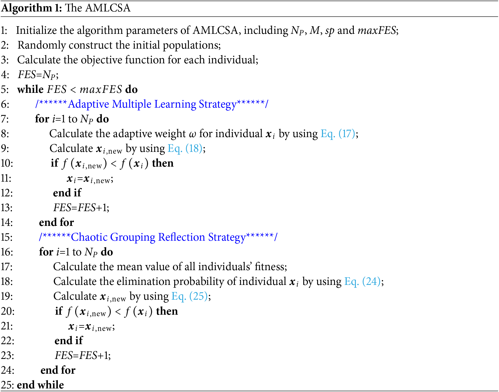
The pseudocode for the AMLCSA algorithm is presented in Algorithm 1, and the flowchart is shown in Fig. 6. First, the algorithm parameters are set, and an initial population is randomly generated. The fitness values of all individuals are then calculated based on the problem. The population is updated using the adaptive multiple learning (AML) and chaotic grouping reflection (CGR) strategies, and better solutions are retained through an elite selection mechanism. This iterative process continues until the termination condition is met. The final output includes the optimal parameters and the optimal objective function values.

Figure 6: Flowchart of the AMLCSA

Time complexity is a crucial metric for evaluating algorithm quality. Below is the time complexity analysis of AMLCSA:

•   Time complexity of the initialization phase: The time complexity of the population initialization phase is O(NPD), where NP is the population size and D is the problem dimension.

•   Time complexity of the initial population fitness evaluation: The time complexity of evaluating the fitness values for all individuals in the population is O(NPTF), where TF is the cost of evaluating a fitness value.

•   Time complexity of the main loop of the algorithm: In the AML strategy, the time complexity for updating the population based on employees’ learning new knowledge is O(NPD), and the time complexity for calculating the adaptive weight is O(NP). In the CGR strategy, the time complexity for updating the population through employees’ self-reflection is O(NPD), and the time complexity for calculating the elimination probability is O(NP). To retain the better individuals, the fitness values of all individuals are calculated after both strategies update the population. Therefore, in one iteration, the time complexity of evaluating fitness values is O(2NPTF). Consequently, the time complexity of the main loop is O(G⋅2NP(TF+D+1)), where G is the maximum number of iterations.

Combining the above time complexities, the total time complexity of AMLCSA is: T=O(NPD)+O(NPTF)+O(G⋅2NP(TF+D+1))≈O(G⋅NP(TF+D)).

5  Experimental Results

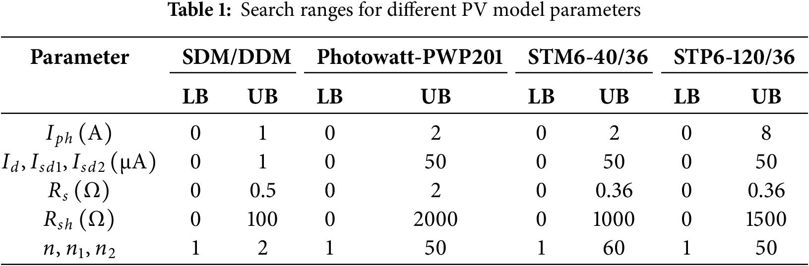
To validate the effectiveness of the proposed AMLCSA, we conduct parameter identification experiments. For the SDM and DDM, data were collected under conditions of 33∘C and 1000 W/m2 for a French R.T.C. commercial silicon solar cell [57]. For the PV modules, three types are tested: the poly-crystalline Photowatt-PWP201 [57], the mono-crystalline STM6-40/36, and the poly-crystalline STP6-120/36 [58,59]. The search ranges for the five PVMPI problems are shown in Table 1.

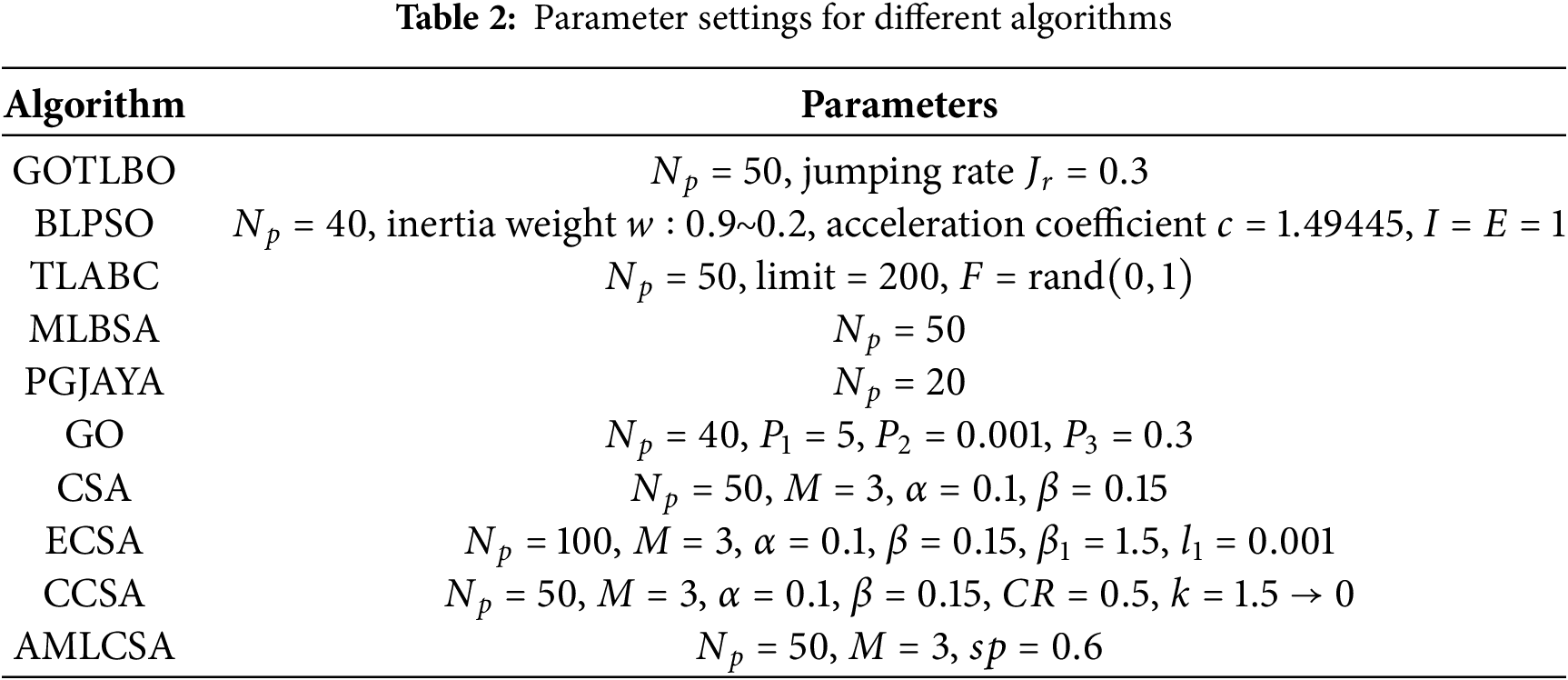
The AMLCSA algorithm is compared with several well-established algorithms, including GOTLBO [29], BLPSO [60], TLABC [30], MLBSA [37], PGJAYA [61], GO [62], CSA [52], ECSA [54], and CCSA [55]2. These algorithms were selected for comparison due to their strong optimization capabilities, which have been proven effective for solving the PVMPI problem. The parameter settings for all the compared algorithms are shown in Table 2, following the values suggested in the respective literature. To minimize statistical errors, each algorithm is run 30 independent times for each PVMPI problem. The maximum functional evaluations (maxFES) for the AMLCSA algorithm are set to 20,000, 20,000, 15,000, 35,000, and 35,000 for the five PVMPI problems, respectively3.

Additionally, for each of the five PVMPI problems, we also select results from recent literature with strong performance for direct comparison, including I-CPA [63], ADHHO [40], SPGWO [64], AOSCS [65], MS-TSA [41], and DIWJAYA [66]. Notably, these studies often use a higher maxFES than ours.

5.1 Results on the SDM PVMPI Problem

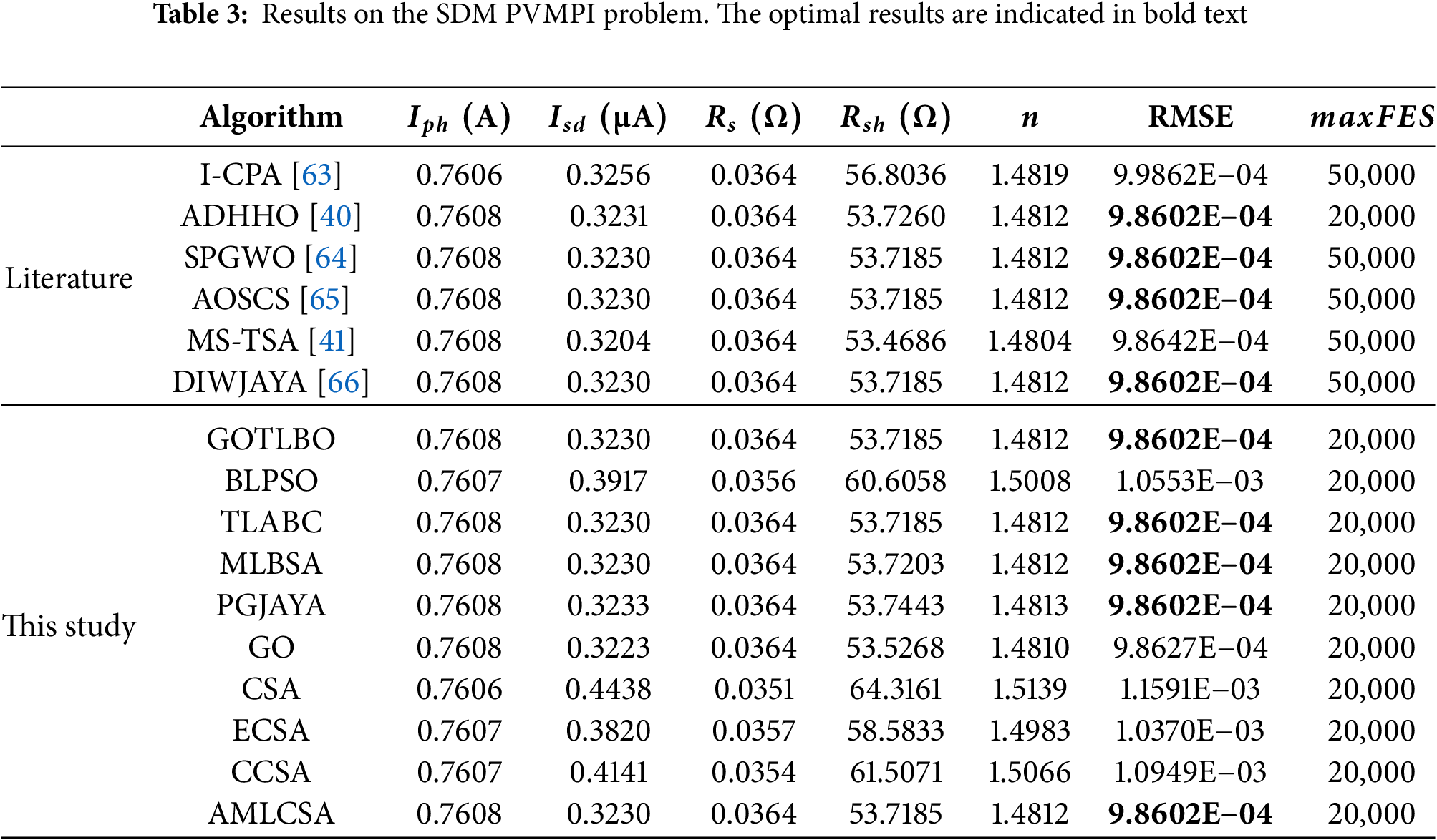
For the SDM PVMPI problem, the parameters and the best RMSE values achieved by the AMLCSA and other algorithms are listed in Table 3, with the best results highlighted in bold. It is evident that AMLCSA, GOTLBO, TLABC, MLBSA, PGJAYA, ADHHO, SPGWO, AOSCS, and DIWJAYA all achieve the best RMSE value of 9.8602E−04. GO achieves the second-best RMSE value (9.8627E−04), followed by MS-TSA (9.8642E−04), I-CPA (9.9862E−04), ECSA (1.0370E−03), BLPSO (1.0553E−03), CCSA (1.0949E−03), and CSA (1.1591E−03). Moreover, while SPGWO, AOSCS, and DIWJAYA achieve the best RMSE of 9.8602E−04, they require a higher maxFES of 50,000.

Since the actual PV model parameters are unavailable, RMSE is used as the primary metric for identification accuracy. The absolute errors (IAE) between simulated and experimental current values, listed in Supplementary Table S14, remain below 1.597E−03, highlighting the high accuracy of AMLCSA.

The optimal parameters obtained by AMLCSA are used to reconstruct the I-V and P-V curves, as shown in Fig. 7. The simulated current values closely match the actual current values across the entire voltage range, demonstrating the accuracy of the parameters obtained via AMLCSA.

Figure 7: Simulated and experimental data using AMLCSA for the SDM model: (a) I-V characteristic curve; (b) P-V characteristic curve

5.2 Results on the DDM PVMPI Problem

The DDM PVMPI problem involves seven unknown parameters, increasing its complexity. Table 4 presents the extracted parameters and RMSE values obtained by AMLCSA and other algorithms. Notably, AMLCSA, AOSCS, and DIWJAYA achieve the best RMSE (9.8248E−04), while ADHHO attains the second-best RMSE (9.8270E−04). However, AOSCS and DIWJAYA require more function evaluations with maxFES=50,000.

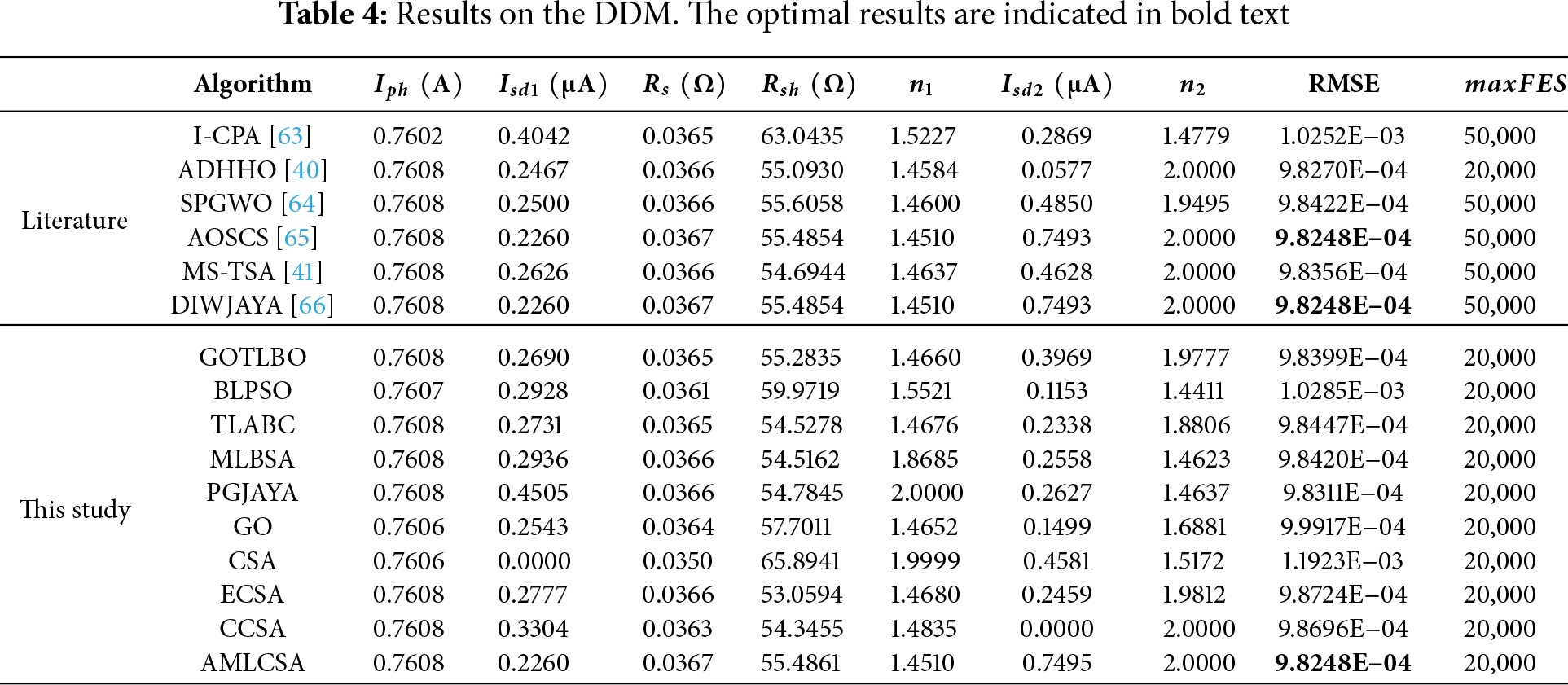
Supplementary Table S2 provides the simulated current values and absolute errors, with an IAE below 1.491E−03, confirming AMLCSA’s identification accuracy. Fig. 8 illustrates the reconstructed I-V and P-V curves, demonstrating strong consistency between simulated and experimental current values.

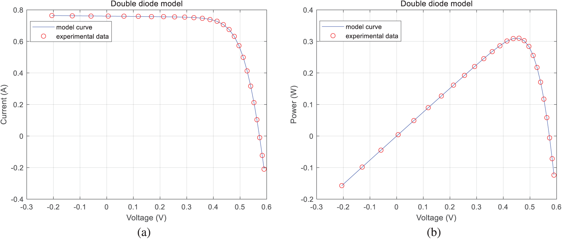
Figure 8: Simulated and experimental data using AMLCSA for the DDM model: (a) I-V characteristic curve; (b) P-V characteristic curve

5.3 Results on the Module PVMPI Problems

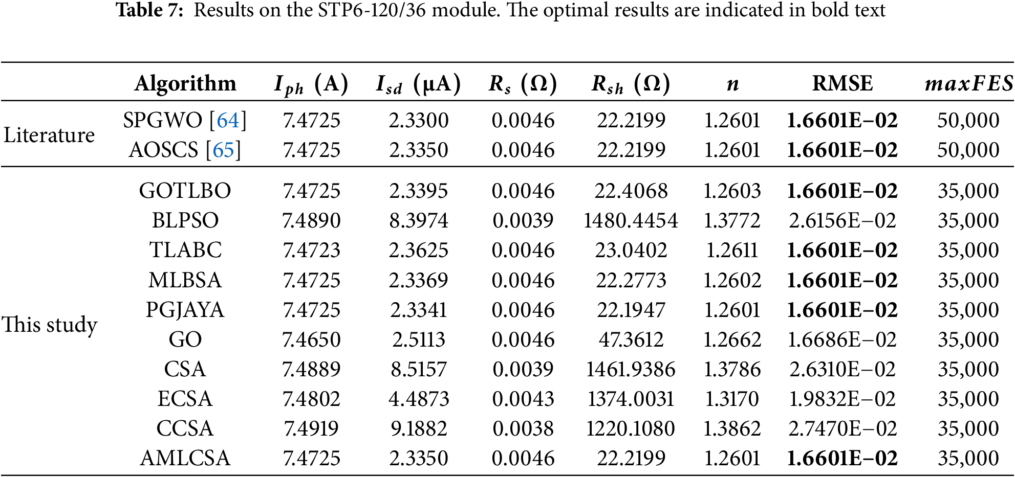
Three different PVMPI module problems are further analyzed to validate AMLCSA. Tables 5–7 present the extracted parameters and optimal RMSE values obtained by AMLCSA and other algorithms for the three PV modules. The results confirm that AMLCSA achieves the lowest RMSE across all modules, demonstrating its effectiveness in parameter identification.

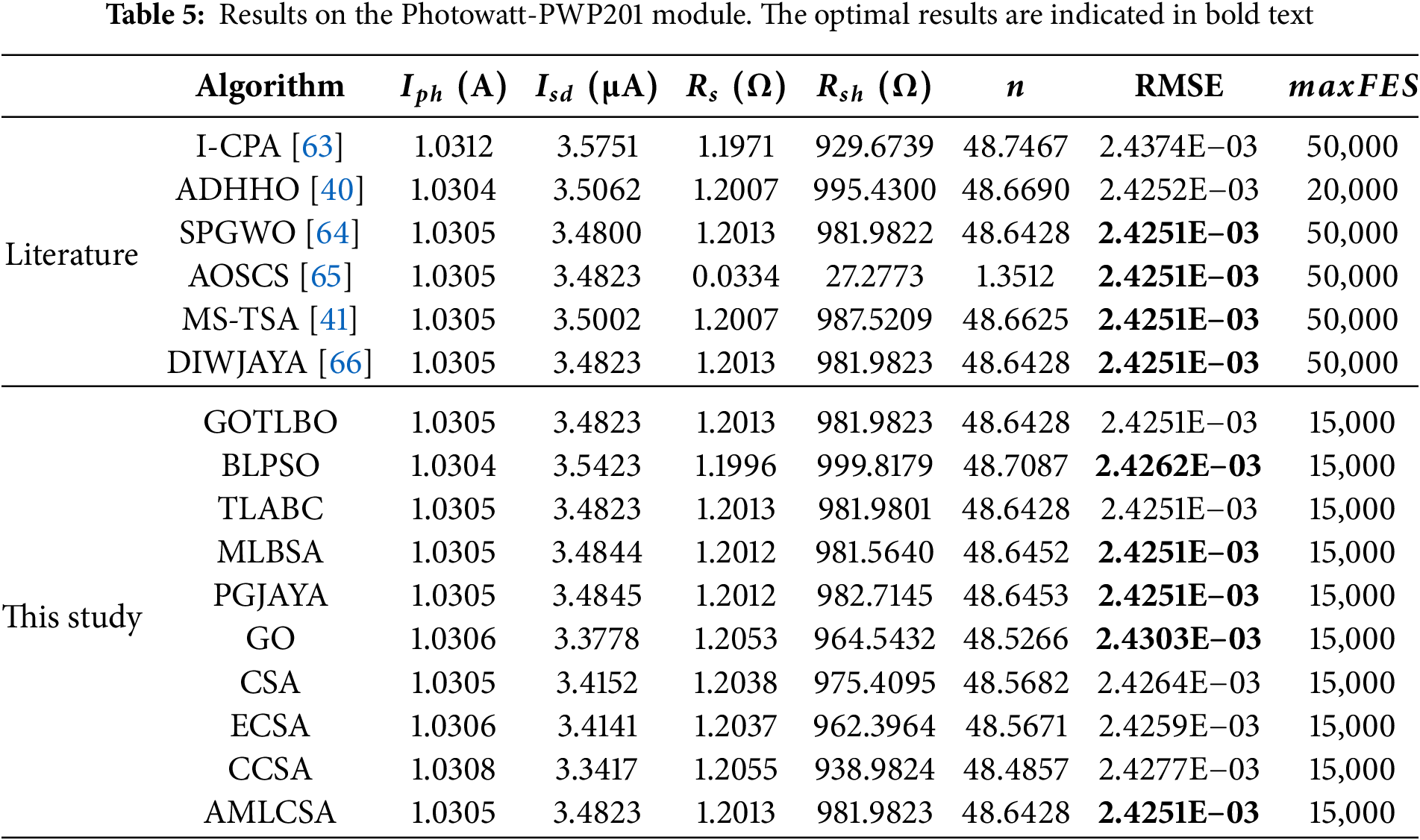
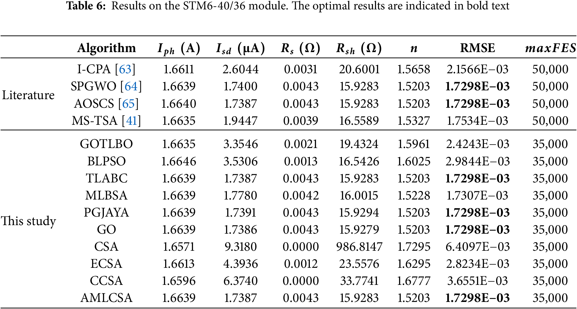
The simulated currents and absolute error values for the three models are provided in Supplementary Tables S3–S5, while the reconstructed I-V and P-V characteristic curves using AMLCSA’s optimal parameters are shown in Figs. 9–11. The simulated data closely matches the experimental data, confirming the high accuracy of AMLCSA’s extracted parameters.

Figure 9: Simulated and experimental data using AMLCSA for the Photowatt-PWP201 module: (a) I-V characteristic curve; (b) P-V characteristic curve

Figure 10: Simulated and experimental data using AMLCSA for the STM6-40/36 module: (a) I-V characteristic curve; (b) P-V characteristic curve

Figure 11: Simulated and experimental data using AMLCSA for the STP6-120/36 module: (a) I-V characteristic curve; (b) P-V characteristic curve

5.4 Statistical Results on Five PVMPI Problems

Since AMLCSA and the competing algorithms are stochastic, comparing their statistical results over multiple independent runs is essential for a comprehensive performance evaluation. Table 8 presents the RMSE statistics after 30 runs, including the minimum, maximum, mean, and standard deviation. Additionally, the Wilcoxon signed-rank test, based on the mean RMSE, was conducted, where a “+” indicates AMLCSA’s significant superiority over its competitors. Finally, the total running time for each algorithm is reported.

For the minimum RMSE, AMLCSA is the only algorithm that achieves the best results across all five PVMPI problems. TLABC and PGJAYA perform best on four problems, excluding DDM, while GOTLBO and MLBSA attain optimal results on three. GO achieves the best result on only one problem, and all other algorithms exhibit inferior performance.

For maximum RMSE, AMLCSA remains the only algorithm to achieve the best results across all five problems, while none of the competing methods reach the best value in any case.

Regarding mean RMSE, AMLCSA demonstrates a significant advantage over all competing algorithms across the five PVMPI problems, indicating its superior average accuracy.

Standard deviation (std) is used as an indicator of solution stability. Table 8 clearly shows that AMLCSA has significantly lower std values compared to other algorithms. Additionally, the Wilcoxon test confirms that AMLCSA substantially outperforms all competitors.

Although AMLCSA does not have the shortest runtime, it achieves optimal results within a relatively short execution time.

Fig. 12 presents the average convergence curves for all algorithms. Compared to its competitors, AMLCSA exhibits faster convergence and higher solution accuracy, demonstrating the efficiency and accuracy of its search process.

Figure 12: Average convergence curves on five PVMPI problems (a) SDM; (b) DDM; (c) Photowatt-PWP201; (d) STM6-40/36; (e) STP6-120/36

In summary, AMLCSA offers higher solution accuracy, better stability, and faster convergence, making it a competitive method for PV parameter identification.

5.5 Influence of Different Components on the AMLCSA Algorithm

AMLCSA incorporates two strategies-AML and CGR-to enhance CSA. To assess their effectiveness, two variants are introduced: (i) AMLCSA-1, which includes CGR but excludes AML, and (ii) AMLCSA-2, which includes AML but excludes CGR. Both variants use the same parameter settings as in the previous section.

Table 9 presents the statistical results of AMLCSA, AMLCSA-1, AMLCSA-2, and basic CSA over 30 runs. The results indicate that basic CSA performs the worst across all PVMPI problems, while embedding either AML or CGR improves performance.

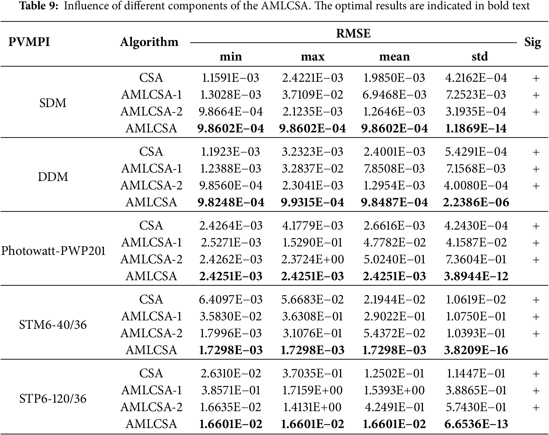
Moreover, AMLCSA outperforms both AMLCSA-1 and AMLCSA-2 across all PVMPI problems, confirming the advantage of combining AML and CGR. Additionally, AMLCSA-2 generally achieves better results than AMLCSA-1, suggesting that AML plays a more significant role in improving solution accuracy. However, AMLCSA-2 still underperforms compared to AMLCSA, demonstrating that CGR is necessary for enhancing population diversity and algorithm stability.

In summary, neither AML nor CGR alone is sufficient to achieve optimal results. Their combination is essential for fully enhancing CSA’s performance. The simulation results confirm that AMLCSA significantly improves solution accuracy, stability, and convergence due to the integration of AML and CGR.

6  Discussion and Conclusion

In this paper, we proposed an adaptive multi-learning cooperative search algorithm (AMLCSA) for accurate and efficient PV model parameter identification (PVMPI). AMLCSA integrates two key strategies: adaptive multi-learning (AML) and chaotic grouping reflection (CGR) strategies. We evaluated AMLCSA on five PVMPI tasks, including SDM, DDM, and three real-world PV modules. The results are compared with those of nine well-known metaheuristic algorithms.

Accuracy and Convergence: Across five PV models (SDM, DDM, and three PV modules), AMLCSA consistently yields lower RMSE values, indicating superior parameter estimation. It also demonstrates faster convergence by attaining high-quality solutions with fewer iterations or function evaluations.

Algorithmic Enhancements: The adaptive multi-learning (AML) strategy dynamically adjusts search intensities, promoting local exploitation using high-performing individuals and encouraging global exploration through lower-performing ones. Additionally, the chaotic grouping reflection (CGR) strategy increases population diversity and mitigates premature convergence. These features enhance AMLCSA’s robustness across varying problem complexities.

Computational Efficiency: The maximum number of function evaluations used for the five models ranges from 15,000 to 35,000, while most algorithms in the literature require 50,000 function evaluations to achieve similar accuracy. The analysis clearly demonstrates that AMLCSA consumes fewer computational resources while achieving comparable or better accuracy than the competing algorithms.

In summary, AMLCSA offers a reliable and efficient solution for PVMPI and holds strong potential for optimizing real-world solar energy systems. Although AMLCSA has shown promising results in PV model parameter identification, there is still potential for optimization, particularly in convergence speed and runtime. In future work, we will focus on further optimizing the AMLCSA algorithm by hybridization with other optimization techniques. Additionally, this paper primarily addresses static PV models. Moving forward, we aim to enhance AMLCSA for online PV parameter identification. We also plan to extend the cooperative search algorithm to tackle the multi-objective PV parameter identification problem.

Acknowledgement: The authors are grateful to all the editors and anonymous reviewers for their comments and suggestions.

Funding Statement: This work was supported by the National Natural Science Foundation of China (Grant Nos. 62303197, 62273214), and the Natural Science Foundation of Shandong Province (ZR2024MFO18).

Author Contributions: Concept and design: Xu Chen and Shuai Wang. Software, validation and visualization: Shuai Wang. Statistical analysis: Shuai Wang. Supervision: Xu Chen. Writing—original draft: Shuai Wang. Writing—review & editing: Xu Chen and Kaixun He. Project administration and resources: Xu Chen and Kaixun He. All authors reviewed the results and approved the final version of the manuscript.

Availability of Data and Materials: Not applicable.

Ethics Approval: Not applicable.

Conflicts of Interest: The authors declare no conflicts of interest to report regarding the present study.

Supplementary Materials: The supplementary material is available online at https://www.techscience.com/doi/10.32604/cmc.2025.066543/s1.

1The effect of parameter sp values on AMLCSA algorithm is discussed in the supplementary file.

2GOTLBO is a generalized opposition learning-based teaching-learning-based optimization algorithm [29]. BLPSO is a biogeography-based learning particle swarm optimization algorithm [60]. TLABC is a hybrid algorithm combining teaching-learning-based optimization and artificial bee colony [30]. MLBSA is a backtracking search algorithm with multiple learning strategies and elite mechanisms [37]. PGJAYA is a JAYA algorithm with a performance-guided evolution strategy [61]. GO is a recent optimizer inspired by the growth process of individuals in society [62]. CSA is a population-based optimization algorithm inspired by teamwork behavior in modern businesses [52]. ECSA is a CSA variant with three improvement strategies [54]. CCSA is an improved algorithm for CSA with the addition of crossover and mutation strategies [55].

3All algorithms were implemented using MATLAB 2021a. The experiments were conducted on a PC with an Intel(R) Core(TM) i7-7700HQ CPU @ 2.80 GHz, 8 GB of RAM, and a 64-bit Windows 10 operating system.

4All the supplementary tables are provided in the supplementary file.

References

1. Gu Q, Li S, Gong W, Ning B, Hu C, Liao Z. L–SHADE with parameter decomposition for photovoltaic modules parameter identification under different temperature and irradiance. Appl Soft Comput. 2023;143(4):110386. doi:10.1016/j.asoc.2023.110386. [Google Scholar] [CrossRef]

2. Deotti LMP, da Silva IC. A survey on the parameter extraction problem of the photovoltaic single diode model from a current–voltage curve. Sol Energy. 2023;263(24):111930. doi:10.1016/j.solener.2023.111930. [Google Scholar] [CrossRef]

3. Elnagi M, Kamel S, Ramadan A, Elnaggar MF. Photovoltaic models parameters estimation based on weighted mean of vectors. Comput Mater Contin. 2023;74(3):5229–50. doi:10.32604/cmc.2023.032469. [Google Scholar] [CrossRef]

4. Gu Z, Xiong G, Fu X. Parameter extraction of solar photovoltaic cell and module models with metaheuristic algorithms: a review. Sustainability. 2023;15(4):3312. doi:10.3390/su15043312. [Google Scholar] [CrossRef]

5. Long W, Jiao J, Liang X, Xu M, Tang M, Cai S. Parameters estimation of photovoltaic models using a novel hybrid seagull optimization algorithm. Energy. 2022;249:123760. doi:10.1016/j.energy.2022.123760. [Google Scholar] [CrossRef]

6. Gu Z, Xiong G, Fu X, Mohamed AW, Al-Betar MA, Chen H, et al. Extracting accurate parameters of photovoltaic cell models via elite learning adaptive differential evolution. Energy Convers Manag. 2023;285(1):116994. doi:10.1016/j.enconman.2023.116994. [Google Scholar] [CrossRef]

7. Chen X, Wang S, He K. Parameter estimation of various PV cells and modules using an improved simultaneous heat transfer search algorithm. J Comput Electron. 2024;23(3):584–99. doi:10.1007/s10825-024-02153-w. [Google Scholar] [CrossRef]

8. Hussain K, Mohd Salleh MN, Cheng S, Shi Y. Metaheuristic research: a comprehensive survey. Artif Intell Rev. 2019;52(4):2191–233. doi:10.1007/s10462-017-9605-z. [Google Scholar] [CrossRef]

9. Ćalasan M, Abdel Aleem SHE, Zobaa AF. On the root mean square error (RMSE) calculation for parameter estimation of photovoltaic models: a novel exact analytical solution based on Lambert W function. Energy Convers Manag. 2020;210:112716. doi:10.1016/j.enconman.2020.112716. [Google Scholar] [CrossRef]

10. Ridha HM, Hizam H, Gomes C, Heidari AA, Chen H, Ahmadipour M, et al. Parameters extraction of three diode photovoltaic models using boosted LSHADE algorithm and Newton Raphson method. Energy. 2021;224(3):120136. doi:10.1016/j.energy.2021.120136. [Google Scholar] [CrossRef]

11. Orioli A, Di Gangi A. A procedure to calculate the five–parameter model of crystalline silicon photovoltaic modules on the basis of the tabular performance data. Appl Energy. 2013;102:1160–77. doi:10.1016/j.apenergy.2012.06.036. [Google Scholar] [CrossRef]

12. Premkumar M, Ravichandran S, Hashim TJT, Sin TC, Abbassi R. Fitness-guided particle swarm optimization with adaptive Newton-Raphson for photovoltaic model parameter estimation. Appl Soft Comput. 2024;167(4):112295. doi:10.1016/j.asoc.2024.112295. [Google Scholar] [CrossRef]

13. Pang Y, Li H, Tang P, Chen C. Synchronization optimization of pipe diameter and operation frequency in a pressurized irrigation network based on the genetic algorithm. Agriculture. 2022;12(5):673. doi:10.3390/agriculture12050673. [Google Scholar] [CrossRef]

14. Chen X, Xu F, He K. Multi–region combined heat and power economic dispatch based on modified group teaching optimization algorithm. International J Electr Power Energy Syst. 2024;155:109586. [Google Scholar]

15. Liu Y, Ding H, Wang Z, Dhiman G, Yang Z, Hu P. An enhanced equilibrium optimizer for solving optimization tasks. Comput Mater Contin. 2023;77(2):2385–406. doi:10.32604/cmc.2023.039883. [Google Scholar] [CrossRef]

16. Gharehchopogh FS. Quantum-inspired metaheuristic algorithms: comprehensive survey and classification. Artif Intell Rev. 2023;56(6):5479–543. doi:10.1007/s10462-022-10280-8. [Google Scholar] [CrossRef]

17. Zhou S, Wang D, Ni Y, Song K, Li Y. Improved particle swarm optimization for parameter identification of permanent magnet synchronous motor. Comput Mater Contin. 2024;79(2):2187–207. doi:10.1109/ipemc-ecceasia60879.2024.10567186. [Google Scholar] [CrossRef]

18. Chen X, Fang S, Li K. Reinforcement–learning–based multi–objective differential evolution algorithm for large–scale combined heat and power economic emission dispatch. Energies. 2023;16(9):3753. doi:10.3390/en16093753. [Google Scholar] [CrossRef]

19. Yu Y, Gao S, Zhou M, Wang Y, Lei Z, Zhang T, et al. Scale–free network–based differential evolution to solve function optimization and parameter estimation of photovoltaic models. Swarm Evol Comput. 2022;74(4):101142. doi:10.1016/j.swevo.2022.101142. [Google Scholar] [CrossRef]

20. Durmus B, Gun A. Development of incremental average differential evolution algorithm for photovoltaic system identification. Sol Energy. 2022;244(7):242–54. doi:10.1016/j.solener.2022.08.046. [Google Scholar] [CrossRef]

21. Wang D, Sun X, Kang H, Shen Y, Chen Q. Heterogeneous differential evolution algorithm for parameter estimation of solar photovoltaic models. Energy Rep. 2022;8(5):4724–46. doi:10.1016/j.egyr.2022.03.144. [Google Scholar] [CrossRef]

22. Abd El-Mageed AA, Abohany AA, Saad HMH, Sallam KM. Parameter extraction of solar photovoltaic models using queuing search optimization and differential evolution. Appl Soft Comput. 2023;134(3):110032. doi:10.1016/j.asoc.2023.110032. [Google Scholar] [CrossRef]

23. Zhang Y, Li S, Wang Y, Yan Y, Zhao J, Gao Z. Self–adaptive enhanced learning differential evolution with surprisingly efficient decomposition approach for parameter identification of photovoltaic models. Energy Convers Manag. 2024;308:118387. doi:10.1016/j.enconman.2024.118387. [Google Scholar] [CrossRef]

24. Abualigah L. Particle swarm optimization: advances, applications, and experimental insights. Comput Mater Contin. 2025;82(2):1539–92. doi:10.32604/cmc.2025.060765. [Google Scholar] [CrossRef]

25. Li Y, Yu K, Liang J, Yue C, Qiao K. A landscape–aware particle swarm optimization for parameter identification of photovoltaic models. Appl Soft Comput. 2022;131(12):109793. doi:10.1016/j.asoc.2022.109793. [Google Scholar] [CrossRef]

26. Fan Y, Wang P, Heidari AA, Chen H, HamzaTurabieh, Mafarja M. Random reselection particle swarm optimization for optimal design of solar photovoltaic modules. Energy. 2022;239(4):121865. doi:10.1016/j.energy.2021.121865. [Google Scholar] [CrossRef]

27. Lu Y, Liang S, Ouyang H, Li S, Wang GG. Hybrid multi–group stochastic cooperative particle swarm optimization algorithm and its application to the photovoltaic parameter identification problem. Energy Reports. 2023;9(3):4654–81. doi:10.1016/j.egyr.2023.03.105. [Google Scholar] [CrossRef]

28. Wang H, Yu X. A ranking improved teaching-learning-based optimization algorithm for parameters identification of photovoltaic models. Appl Soft Comput. 2024;167:112371. doi:10.1016/j.asoc.2024.112371. [Google Scholar] [CrossRef]

29. Chen X, Yu K, Du W, Zhao W, Liu G. Parameters identification of solar cell models using generalized oppositional teaching learning based optimization. Energy. 2016;99(9):170–80. doi:10.1016/j.energy.2016.01.052. [Google Scholar] [CrossRef]

30. Chen X, Xu B, Mei C, Ding Y, Li K. Teaching–learning–based artificial bee colony for solar photovoltaic parameter estimation. Appl Energy. 2018;212:1578–88. doi:10.1016/j.apenergy.2017.12.115. [Google Scholar] [CrossRef]

31. Duman S, Kahraman HT, Sonmez Y, Guvenc U, Kati M, Aras S. A powerful meta–heuristic search algorithm for solving global optimization and real–world solar photovoltaic parameter estimation problems. Eng Appl Artif Intell. 2022;111(3):104763. doi:10.1016/j.engappai.2022.104763. [Google Scholar] [CrossRef]

32. Yu K, Qu B, Yue C, Ge S, Chen X, Liang J. A performance–guided JAYA algorithm for parameters identification of photovoltaic cell and module. Appl Energy. 2019;237:241–57. [Google Scholar]

33. Zhang Y, Ma M, Jin Z. Comprehensive learning Jaya algorithm for parameter extraction of photovoltaic models. Energy. 2020;211:118644. doi:10.1016/j.energy.2020.118644. [Google Scholar] [CrossRef]

34. Jian X, Cao Y. A chaotic second order oscillation Jaya algorithm for parameter extraction of photovoltaic models. Photonics. 2022;9(3):131. doi:10.3390/photonics9030131. [Google Scholar] [CrossRef]

35. Askarzadeh A, Rezazadeh A. Parameter identification for solar cell models using harmony search–based algorithms. Sol Energy. 2012;86(11):3241–9. doi:10.1016/j.solener.2012.08.018. [Google Scholar] [CrossRef]

36. Luo W, Yu X. Quasi–reflection based multi–strategy cuckoo search for parameter estimation of photovoltaic solar modules. Sol Energy. 2022;243(4):264–78. doi:10.1016/j.solener.2022.08.004. [Google Scholar] [CrossRef]

37. Yu K, Liang JJ, Qu BY, Cheng Z, Wang H. Multiple learning backtracking search algorithm for estimating parameters of photovoltaic models. Appl Energy. 2018;226:408–22. doi:10.1016/j.apenergy.2018.06.010. [Google Scholar] [CrossRef]

38. Liu Y, Heidari AA, Ye X, Liang G, Chen H, He C. Boosting slime mould algorithm for parameter identification of photovoltaic models. Energy. 2021;234(5):121164. doi:10.1016/j.energy.2021.121164. [Google Scholar] [CrossRef]

39. Wang J, Yang B, Li D, Zeng C, Chen Y, Guo Z, et al. Photovoltaic cell parameter estimation based on improved equilibrium optimizer algorithm. Energy Convers Manag. 2021;236(3):114051. doi:10.1016/j.enconman.2021.114051. [Google Scholar] [CrossRef]

40. Song S, Wang P, Heidari AA, Zhao X, Chen H. Adaptive Harris hawks optimization with persistent trigonometric differences for photovoltaic model parameter extraction. Eng Appl Artif Intell. 2022;109(13):104608. doi:10.1016/j.engappai.2021.104608. [Google Scholar] [CrossRef]

41. Beşkirli A, Dağ İ, Kiran MS. A tree seed algorithm with multi-strategy for parameter estimation of solar photovoltaic models. Appl Soft Comput. 2024;167:112220. doi:10.1016/j.asoc.2024.112220. [Google Scholar] [CrossRef]

42. Abdel-Basset M, El-Shahat D, Sallam KM, Munasinghe K. Parameter extraction of photovoltaic models using a memory–based improved gorilla troops optimizer. Energy Convers Manag. 2022;252:115134. doi:10.1016/j.enconman.2021.115134. [Google Scholar] [CrossRef]

43. Kumar C, Magdalin Mary D. A novel chaotic–driven Tuna Swarm Optimizer with Newton–Raphson method for parameter identification of three–diode equivalent circuit model of solar photovoltaic cells/modules. Optik. 2022;264(3):169379. doi:10.1016/j.ijleo.2022.169379. [Google Scholar] [CrossRef]

44. Huang T, Zhang C, Ouyang H, Luo G, Li S, Zou D. Parameter identification for photovoltaic models using an improved learning search algorithm. IEEE Access. 2020;8:116292–309. doi:10.1109/access.2020.3003814. [Google Scholar] [CrossRef]

45. Arandian B, Eslami M, Khalid SA, Khan B, Sheikh UU, Akbari E, et al. An effective optimization algorithm for parameters identification of photovoltaic models. IEEE Access. 2022;10:34069–84. doi:10.1109/access.2022.3161467. [Google Scholar] [CrossRef]

46. Yaghoubi M, Eslami M, Noroozi M, Mohammadi H, Kamari O, Palani S. Modified salp swarm optimization for parameter estimation of solar PV models. IEEE Access. 2022;10(2):110181–94. doi:10.1109/access.2022.3213746. [Google Scholar] [CrossRef]

47. Eslami M, Akbari E, Seyed Sadr ST, Ibrahim BF. A novel hybrid algorithm based on rat swarm optimization and pattern search for parameter extraction of solar photovoltaic models. Energy Sci Eng. 2022;10(8):2689–713. doi:10.1002/ese3.1160. [Google Scholar] [CrossRef]

48. Bo Q, Cheng W, Khishe M, Mohammadi M, Mohammed AH. Solar photovoltaic model parameter identification using robust niching chimp optimization. Sol Energy. 2022;239(7):179–97. doi:10.1016/j.solener.2022.04.056. [Google Scholar] [CrossRef]

49. Sharma A, Sharma A, Averbukh M, Rajput S, Jately V, Choudhury S, et al. Improved moth flame optimization algorithm based on opposition–based learning and Lévy flight distribution for parameter estimation of solar module. Energy Rep. 2022;8:6576–92. doi:10.1016/j.egyr.2022.05.011. [Google Scholar] [CrossRef]

50. El-Dabah MA, El-Sehiemy RA, Hasanien HM, Saad B. Photovoltaic model parameters identification using Northern Goshawk Optimization algorithm. Energy. 2023;262:125522. doi:10.1016/j.energy.2022.125522. [Google Scholar] [CrossRef]

51. Słowik A, Cpałka K, Xue Y, Hapka A. An efficient approach to parameter extraction of photovoltaic cell models using a new population-based algorithm. Appl Energy. 2024;364(1):123208. doi:10.1016/j.apenergy.2024.123208. [Google Scholar] [CrossRef]

52. Feng Z, Niu W, Liu S. Cooperation search algorithm: a novel metaheuristic evolutionary intelligence algorithm for numerical optimization and engineering optimization problems. Appl Soft Comput. 2021;98:106734. doi:10.1016/j.asoc.2020.106734. [Google Scholar] [CrossRef]

53. Niu W, Feng Z, Li Y, Liu S. Cooperation search algorithm for power generation production operation optimization of cascade hydropower reservoirs. Water Resour Manag. 2021;35(8):2465–85. doi:10.1007/s11269-021-02842-2. [Google Scholar] [CrossRef]

54. Jiang Z, Duan J, Xiao Y, He S. Elite collaborative search algorithm and its application in power generation scheduling optimization of cascade reservoirs. J Hydrol. 2022;615(15):128684. doi:10.1016/j.jhydrol.2022.128684. [Google Scholar] [CrossRef]

55. Cao H, Zheng H, Hu G. An improved cooperation search algorithm for the multi–degree reduction in ball Bézier surfaces. Soft Comput. 2023;27(16):11687–714. doi:10.1007/s00500-023-07847-0. [Google Scholar] [CrossRef]

56. Ali F, Sarwar A, Ilahi Bakhsh F, Ahmad S, Ali Shah A, Ahmed H. Parameter extraction of photovoltaic models using atomic orbital search algorithm on a decent basis for novel accurate RMSE calculation. Energy Convers Manag. 2023;277(1):116613. doi:10.1016/j.enconman.2022.116613. [Google Scholar] [CrossRef]

57. Easwarakhanthan T, Bottin J, Bouhouch I, Boutrit C. Nonlinear minimization algorithm for determining the solar cell parameters with microcomputers. Int J Sol Energy. 1986;4(1):1–12. doi:10.1080/01425918608909835. [Google Scholar] [CrossRef]

58. Tong NT, Pora W. A parameter extraction technique exploiting intrinsic properties of solar cells. Appl Energy. 2016;176:104–15. doi:10.1016/j.apenergy.2016.05.064. [Google Scholar] [CrossRef]

59. Gao X, Cui Y, Hu J, Xu G, Wang Z, Qu J, et al. Parameter extraction of solar cell models using improved shuffled complex evolution algorithm. Energy Conv Manag. 2018;157:460–79. doi:10.1016/j.enconman.2017.12.033. [Google Scholar] [CrossRef]

60. Chen X, Tianfield H, Mei C, Du W, Liu G. Biogeography–based learning particle swarm optimization. Soft Comput. 2016;21(24):7519–41. doi:10.1007/s00500-016-2307-7. [Google Scholar] [CrossRef]

61. Li S, Gong W, Yan X, Hu C, Bai D, Wang L, et al. Parameter extraction of photovoltaic models using an improved teaching–learning–based optimization. Energy Conv Manag. 2019;186(7):293–305. doi:10.1016/j.enconman.2019.02.048. [Google Scholar] [CrossRef]

62. Zhang Q, Gao H, Zhan ZH, Li J, Zhang H. Growth Optimizer: a powerful metaheuristic algorithm for solving continuous and discrete global optimization problems. Knowl Based Syst. 2023;261(3):110206. doi:10.1016/j.knosys.2022.110206. [Google Scholar] [CrossRef]

63. Beşkirli A, Dağ İ. I-CPA: an improved carnivorous plant algorithm for solar photovoltaic parameter identification problem. Biomimetics. 2023;8(8):569. doi:10.3390/biomimetics8080569. [Google Scholar] [PubMed] [CrossRef]

64. Yu X, Duan Y, Cai Z. Sub–population improved grey wolf optimizer with Gaussian mutation and Lévy flight for parameters identification of photovoltaic models. Expert Syst Appl. 2023;232:120827. doi:10.1016/j.eswa.2023.120827. [Google Scholar] [CrossRef]

65. Yang Q, Wang Y, Zhang J, Gao H. An adaptive operator selection cuckoo search for parameter extraction of photovoltaic models. Appl Soft Comput. 2024;166:112221. doi:10.1016/j.asoc.2024.112221. [Google Scholar] [CrossRef]

66. Choulli I, Elyaqouti M, Saadaoui D, Lidaighbi S, Elhammoudy A, Abazine I, et al. DIWJAYA: JAYA driven by individual weights for enhanced photovoltaic model parameter estimation. Energy Convers Manag. 2024;305:118258. doi:10.1016/j.enconman.2024.118258. [Google Scholar] [CrossRef]