A Deep Learning-Based Cloud Groundwater Level Prediction System

1  Introduction

With the development of various industries, global reliance on groundwater resources has significantly increased to meet the demands of domestic water use, agricultural irrigation, and industrial production. However, excessive and unregulated extraction has led to a growing shortage of water and has triggered serious environmental issues worldwide, including land subsidence and seawater intrusion. These phenomena not only damage infrastructure and cause salinization of water sources, but also negatively impact agricultural productivity and land use. Several studies haves shown that excessive groundwater extraction directly leads to sediment compaction, which is the primary cause of environmental problems such as land subsidence [1]. To improve the effectiveness of groundwater resource management, an increasing number of studies are focusing on simulating groundwater level changes and integrating various monitoring and prediction techniques to develop more comprehensive forecasting systems.

The rapid development of Internet of Things (IoT) and cloud computing has motivated several studies to explore the feasibility of implementing models in cloud-based environments. These systems collected real-time data through sensors and transmitted them to the cloud for storage and preliminary analysis, aiming to achieve more effective monitoring [2]. However, constructing a forecasting system that offers both high accuracy and interpretability based on large-scale data remains a key challenge in current research. In the past, groundwater level prediction was primarily based on statistical models. However, with the emergence of IoT technology, an increasing number of sensors have been deployed to monitor groundwater levels and hydrological parameters [3]. In addition, recent advancements in artificial intelligence (AI) have enabled the real-time analysis of large volumes of data collected from sensors and other sources, helping researchers make more informed decisions.

To improve the accuracy of groundwater modeling under massive and complex datasets, it has become essential to identify patterns and relationships among diverse data sources. As a result, recent studies have adopted various machine learning techniques, including Decision Tree, Random Forest, Support Vector Machine (SVM), and Artificial Neural Networks (ANN). Despite traditional ML widespread use, conventional machine learning models generally struggle to retain temporal context, which limits their capacity to capture extended dependencies across time-series sequences. To address the challenges of capturing both short and long-term dependencies as well as nonlinear relationships in time series forecasting, researchers have proposed recurrent neural networks (RNNs) and their variants, such as Long Short-Term Memory (LSTM), which are equipped with memory units to enhance the mapping capability of complex multi-scale data [4]. Consequently, RNN and LSTM architectures have gained popularity for modeling the temporal behavior of groundwater systems, particularly in tasks involving water level forecasting [5,6]. In the context of long-term groundwater forecasting, further studies have introduced the Bidirectional Long Short-Term Memory (BiLSTM) model to improve the model’s ability to capture temporal features. The BiLSTM model is capable of simultaneously considering past and future information in a sequence, thereby outperforming LSTM in time series prediction tasks [7]. Recent studies have applied BiLSTM to groundwater forecasting and have shown that it can produce more accurate and stable predictions over different forecast periods [8].

This study focuses on the Zhuoshui River alluvial fan area, where groundwater has long been a primary source for agricultural irrigation and domestic water use. Groundwater levels in this region are affected by multiple factors, including river recharge, groundwater extraction, and rainfall variability. Although the proposed model does not explicitly incorporate hydrogeological parameters, the deep learning framework is designed to learn underlying patterns from long-term observational data and capture complex temporal dependencies. This research builds upon our previous work in the same region, where AI techniques were used to simulate groundwater levels and evaluate the impact of pumping activities [9]. In the present study, we further enhance the forecasting model architecture and data processing pipeline to better capture trend variations across different time intervals and to improve predictive stability.

Building upon these regional challenges and data characteristics, this study presents a groundwater level forecasting system that integrates a cloud-based data management framework with deep learning models. While cloud-based platforms have been widely used in hydrological data environments, the core contribution of this study does not lie in the use of cloud infrastructure itself, but rather in the integration of lightweight, anomaly-aware statistical preprocessing with a deep learning forecasting pipeline. Specifically, the system first performs data imputation using seasonal-trend decomposition and STL-SARIMA techniques, with the processed data stored in a cloud environment to facilitate scalable model training. Subsequently, three deep learning models—RNN, LSTM, and BiLSTM—are then optimized using Bayesian search, and their forecasting results are systematically compared and evaluated.

This integrated workflow demonstrates the proposed approach’s ability to improve prediction accuracy under noisy and incomplete hydrological conditions. The findings highlight a practical and extensible framework that seamlessly integrates statistical preprocessing and deep learning into a cohesive system for groundwater resource monitoring and sustainable water resource management. This design enables the model to effectively address real-world challenges such as incomplete monitoring records and seasonal fluctuations, while maintaining high accuracy and stability. Furthermore, the study demonstrates the model’s adaptability to location-specific characteristics.

2  Literature Review

In groundwater level forecasting research, data quality and model selection are key factors that influence predictive performance. This section presents a literature review of data preprocessing techniques and commonly used groundwater forecasting models, organized according to the forecasting workflow proposed in this study.

2.1 Data Preprocessing: Outlier Detection and Data Imputation

In time-series analysis, outlier detection identifies unusual data points that deviate from general temporal patterns. Such anomalies may result from sudden events, sensor malfunctions, or human errors. If not properly addressed, outliers can introduce errors during the training or cause significant deviations during prediction. Removing or correcting these anomalous values helps improve data quality and results in a cleaner dataset, which in turn enhances the accuracy of subsequent forecasting [10].

Statistical methods were among the earliest approaches used for outlier detection. Grubbs [11] introduced a Z-score-based method that quantifies the deviation of a data point from the mean, particularly effective for large datasets.

In terms of data imputation, previous studies found that SARIMA outperformed traditional statistical forecasting models in fitting seasonal and periodic data. Valipour [12] demonstrated that the SARIMA model performed better than the ARIMA model in predicting annual runoff. Lee and Kim [13] further revealed that combining STL with SARIMA surpassed other neural network models in outlier detection tasks, providing more accurate prediction outcomes. Similarly, Tejada et al. [14] demonstrated that SARIMA effectively captures variations in short-term seasonal water level predictions, leading to improved forecasting accuracy.

To efficiently process groundwater time-series data, this study adopts lightweight statistical methods for anomaly detection and imputation. Outlier detection uses a Z-score method with a sliding window, which identifies anomalies without model training. For imputation, SARIMA combined with seasonal-trend decomposition ensures temporal continuity and is suitable for edge hardware with limited resources, aligning with real-time data processing requirements. This approach not only aligns with the temporal characteristics of groundwater data but also meets the practical constraints of real-time data processing in resource-constrained settings.

2.2 Evolution of Groundwater Forecasting Models

Early hydrological forecasting relied on linear models such as multiple regression and ARIMA. However, Adamowski et al. [15] noted that their linear assumptions limited their ability to capture nonlinear patterns, resulting in poor predictive performance. In contrast, ANNs are more effective at modeling nonlinear relationships, thereby improving accuracy.

In recent years, advancements in sensing technologies have enabled groundwater monitoring systems to continuously collect large volumes of data from different wells, time periods, and hydrological variables, generating a wider range of influencing factors that must be analyzed for effective forecasting [16]. Previous predictive models were constrained by surface-level data relationships and were unable to detect more intricate patterns, leading to predictions that lacked accuracy. Hinton et al. [17] introduced Deep Belief Networks (DBNs) as an unsupervised learning method. The key advantage of DBNs is their capacity to capture deep, complex, and nonlinear relationships by leveraging hierarchical feature representations. Among these, RNNs were widely recognized as effective approaches for capturing sequential dependencies in data [18]. However, subsequent studies found that traditional RNNs are only suitable for predicting short sequences. When handling long sequence data, they are prone to issues such as gradient vanishing or gradient explosion due to the inability to retain long-term information [19].

To address the challenges faced by standard RNNs in retaining information over extended sequences, Hochreiter and Schmidhuber [20] developed the LSTM model. The model uses the cell state to store information over longer time spans, enabling it to build more effective models for predicting long-sequence data. To enhance stability, Gers et al. [21] added a forget gate to the LSTM, allowing the model to decide whether to retain information from the previous cell state, thereby further improving its predictive performance. The LSTM model has been widely applied in groundwater and hydrological forecasting research. Zhang et al. [22] used an LSTM model to predict water level variations in an agricultural region of China, successfully capturing both long-term trends and short-term fluctuations. Similarly, Le et al. [18] applied LSTM to groundwater and river flow prediction in Vietnam, while Patra and Chu [23] demonstrated the effectiveness of a CNN-LSTM hybrid model for groundwater forecasting in Taiwan’s Choushui River Alluvial Fan. All studies reported that LSTM significantly outperformed traditional models in handling nonlinearity and long-term dependencies, demonstrating strong potential for practical applications.

2.3 Applications of the BiLSTM Model in Groundwater Forecasting

Based on the LSTM architecture, Baziotis et al. [24] introduced the BiLSTM network. This model builds on LSTM by adding a reverse LSTM layer, transforming the unidirectional processing of sequential data into a bidirectional approach, thereby capturing more comprehensive temporal dependencies. Siami-Namini et al. [7] also suggested that BiLSTM is better suited than LSTM for time-series data analysis. In the review by Ali et al. [25], a substantial number of studies applying BiLSTM models to groundwater level forecasting were also identified.

BiLSTM has been employed to address groundwater prediction problems in various regions. For example, Ghasemlounia et al. [26] employed a BiLSTM-based framework to forecast groundwater level fluctuations in four wells located in the West Azerbaijan region. Their model demonstrated reasonable and accurate predictions under different water resource management scenarios. Similarly, Vu et al. [8] applied BiLSTM for predicting river flow and groundwater levels in the Normandy region of western France, achieving prediction errors between 3% and 5% for varying time horizons.

In summary, the BiLSTM model demonstrates strong potential for handling sequential data characterized by temporal dependencies and nonlinear features. It is particularly suitable for forecasting tasks involving long durations and high variability, such as groundwater level prediction. Based on this, the present study adopted BiLSTM as the primary forecasting model and included traditional RNN and LSTM models for systematic comparison. This selection is grounded in the evolutionary relationship and architectural differences among the three models in time-series forecasting, allowing for an effective assessment of their respective abilities in capturing long-term dependencies and extracting relevant features. This comparison aims to identify the most suitable model architecture for predicting groundwater level variations.

To ensure consistency and fairness in model comparison, all models were trained using the same input data, procedures, and evaluated metrics. In addition, to further enhance model performance and adaptability, this study incorporated hyperparameter optimization techniques to improve learning effectiveness and generalization capability.

3  Method

This study proposed a groundwater level prediction system integrated with a cloud storage architecture. The overall workflow is divided into four main modules: Data Collection, Imputation, Model Training, and Performance Evaluation, each described in detail below.

The system began with data collection, where sensors measured river and groundwater levels and transmitted the data to sensor nodes. These nodes performed initial preprocessing and prediction, then forwarded both the raw data and results to the Cloud Center, which managed storage and analyzed predictions. The cloud infrastructure in this study builds upon prior developments in IoT-based hydrological monitoring [27].

In the imputation stage, missing values caused by sensor failure or environmental factors are addressed. Outliers are detected using a Z-score method with a sliding window, and gaps are filled via SARIMA models combined with STL decomposition to ensure temporal continuity.

During training, the preprocessed dataset is divided into separate subsets for model development and evaluation. These subsets are then used to train RNN, LSTM, and BiLSTM architectures. Bayesian Optimization is applied to fine-tune hyperparameters and enhancing both performance stability and accuracy. In the final evaluation stage, model performance was assessed using metrics such as Mean Squared Error (MSE) and R2. The results provided insights into the model’s suitability for groundwater forecasting and serve as a decision support reference for resource management.

3.1 Data Collection

3.1.1 Study Area

The Zhuoshui River alluvial fan, also known as the Zhuoshui River Plain, is the largest alluvial plain in Taiwan, located in the central western region spanning Changhua and Yunlin counties [28]. It covers approximately 2100 km2, bounded by the Wu River in the north, Beigang River in the south, the Bagua Plateau and Douliu Hills in the east, and the Taiwan Strait in the west. Flowing from east to west, the Zhuoshui River significantly influences groundwater replenishment and mediates interactions between surface and subsurface water systems. To enhance the spatial interpretability of the forecasting models, the spatial relationship between river and groundwater monitoring stations was considered during station selection. Although this study did not quantitatively analyze upstream–downstream interactions, previous research has identified time-lagged relationships between river levels and groundwater responses, suggesting hydrological connectivity.

3.1.2 Dataset Description and Feature Selection

The dataset used in this study covers groundwater and river water level observations from January 2020 to December 2023, spanning a total of four years (48 months). Hydrological data were sourced from the public portal maintained by the Water Resources Agency, Ministry of Economic Affairs, Taiwan. The groundwater dataset includes records from 766 monitoring wells across Taiwan, while river water level data were collected from approximately 252 gauging stations. All data are high-frequency observations recorded at 10-min intervals.

The raw CSV files were downloaded using a web crawler and were filtered by geographic location to retain only monitoring stations within the Zhuoshui River alluvial fan area. A total of 197 groundwater level stations and 16 river stage stations within the study area were selected as the basis for subsequent model training and analysis.

3.2 Data Imputation

Outlier Detection & Missing Value Imputation

The overall imputation process in this study is divided into three main stages:

First, Outlier detection was performed on the raw time-series data using a Z-score–based statistical method with a six-point sliding window. The mean of the first five points was used as a reference to evaluate the sixth. If the absolute deviation exceeded a fixed threshold of 4.0, the value was treated as an outlier and was replaced by the local mean. This lightweight method efficiently identified short-term anomalies without requiring model training or parameter tuning.

Next, the identified abnormal and missing segments were processed using STL decomposition, which separated the time series into trend, seasonal, and residual components to preserved both short-term patterns and long-term trends. For each missing interval, STL was applied to the preceding 90 data points with a seasonal cycle of 7, reflecting weekly fluctuations in groundwater levels. The extracted trend component was then used to train a SARIMA model, whose order parameters (p,d,q) and seasonal terms (P,D,Q,s) were automatically determined via the auto_arima function based on AIC minimization. The forecasted values were combined with the original seasonal and residual components to reconstruct the complete time series and restored missing or anomalous values while maintaining data continuity.

3.3 Model Construction and Training

3.3.1 Input Preprocessing

During the model training phase, the imputed groundwater and river water level data were used as input sources, and preprocessing procedures were applied to enhance training efficiency and accuracy. For the groundwater level data, the 10-min observation records were first aggregated into daily averages based on their timestamps. This step helped smooth short-term fluctuations and strengthen trend-related features. River stage data were processed using the same method to ensure the consistency and comparability of the two datasets.

In addition, to prevent discrepancies in feature scales from affecting model training, the river water level data were normalized. Min-Max normalization was applied to scale the values to the [0, 1] range, which accelerated model convergence and stabilized the gradient update process. After completing the above preprocessing steps, the data were ready to be used for model training.

3.3.2 Model Architecture (RNN, LSTM, BiLSTM)

To evaluate the predictive performance of different deep learning architectures on groundwater level time-series data, this study compared three models: RNN, LSTM, and BiLSTM. These models are all capable of capturing temporal dependencies, dynamic variations, and long-term correlations, and have been widely used in hydrological forecasting.

The selection is based on their architectural characteristics: RNN offers a simple structure and fast training, serving as a baseline; LSTM is well-established in time-series forecasting and effective for data with trends and seasonality; BiLSTM incorporates both forward and backward temporal information, enhancing sensitivity to long-term dependencies and multivariate influences, making it suitable for more complex hydrological scenarios. Each model was trained using identical input data and within the same parameter constraints. Their forecasting accuracy was then evaluated based on a shared set of performance metrics.

3.3.3 Hyperparameter Optimization

To obtain the best solution for our chosen model, the model’s hyperparameters were adjusted using the Bayesian optimization Algorithm 1. Bayesian optimization was employed as a method for optimizing expensive evaluation functions, often utilizing Gaussian processes for efficient optimization. This approach was particularly suitable for hyperparameter tuning of deep learning models that required extensive computing resources [29]. Compared with random search and grid search, Bayesian optimization optimizes by iteratively calculating the posterior distribution that best described the objective function, enabling it to find approximately optimal solutions with limited evaluations [30].

Algorithm 1 was based on Bayesian statistics and Gaussian processes. It establishes a probability model in the hyperparameter space and gradually optimizes the objective function. The flow of the SMBO algorithm is as follows: First, a probabilistic model M is established. Each training uses λ as the parameter of the model candidate configuration. Repeated verification and evaluation of the generalization ability of the hyperparameters of this training are performed. The relationship between λ and the score c of the objective function is added to the observation history set H, and the model was continuously updated until the process was completed.

For implementation, this study employed the Keras Tuner tool [31] with Bayesian optimization over 30 iterations to balance convergence speed and computational cost. After defining the search space, automated tuning adjusted critical hyperparameters, including hidden units, layer depth, dropout rate, learning rate, and batch size. These configurations were explored to capture complex temporal dependencies while controlling overfitting. At each iteration, suboptimal combinations were discarded, and the best-performing setup was selected for final training. Table 1 summarizes the key hyperparameters and their search ranges.

3.4 Model Evaluation

To evaluate the performance of the three deep learning models in groundwater level forecasting tasks, this study adopted two commonly used and representative regression evaluation metrics: the coefficient of determination (R2) and mean squared error (MSE). The R2 metric indicates the extent to which model predictions align with actual observations, quantifying the proportion of total variance explained by the model. MSE measures the magnitude of errors between predicted and actual values during the forecasting process. R2 and MSE are commonly used metrics for evaluating the performance of groundwater level prediction models, providing a reliable assessment of model accuracy and robustness [32].

The formulas are presented as follows:

Let xi denote the i-th predicted groundwater level, yi denote the i-th observed groundwater level, and m be the total number of samples. Let y^ represent the mean of the observed groundwater levels.

y^=1m∑i=1nyi(1)

The R2 is defined as:

R2=1−∑i=1n(xi−yi)2∑i=1n(y^−yi)2(2)

MSE is defined as:

MSE=1m∑i=1m(xi−yi)2(3)

To evaluate model performance, the prediction results generated by the three approaches are examined and compared based on two key indicators.

4  Results

4.1 Data Selection Results

To establish representative training and testing datasets for model development, this study focused on the Zhuoshui River Basin and selected pairs of river and groundwater monitoring stations with upstream-downstream geographical relationships. Initially, five station pairs with potential hydrological correspondence were identified.

After data screening and quality assessment, the final selection included the Xiutan Groundwater Observation Well and the Tukou Bridge River Gauge Station, which served as the primary data sources for model training and prediction. This pairing was chosen to explore the dynamic relationship between groundwater and river water levels.

4.2 Data Imputation Results

This study performed outlier detection and missing data imputation on long-term records from the Xiutan groundwater observation well and the Tukou Bridge river level station, which contained extended gaps and anomalous spikes due to sensor failures and communication interruptions. To improve data completeness and continuity for model training, anomalies were identified using a Z-score method with a sliding window. Marked segments were then reconstructed using STL decomposition followed by SARIMA modeling of the trend component.

Figs. 1 and 2 show the imputation results for the Tukou Bridge and Xiutan stations, respectively. In each figure, the blue line represents the original data, red dots indicate missing values, and the green dashed lines denote the reconstructed segments. The results demonstrate that the imputation process successfully filled multiple prominent gaps while maintaining reasonable continuity in both the overall trend and the magnitude of variations.

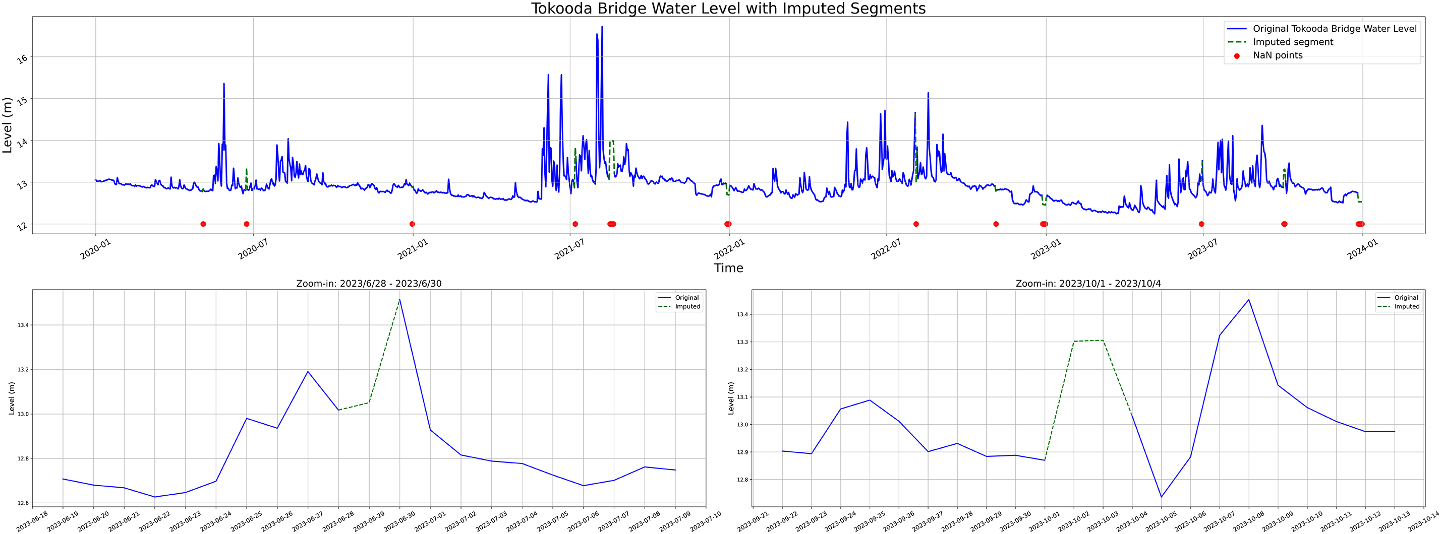
Figure 1: River water level imputation results at Tukou Bridge (2020–2023). Enlarged views of two imputation segments are shown below

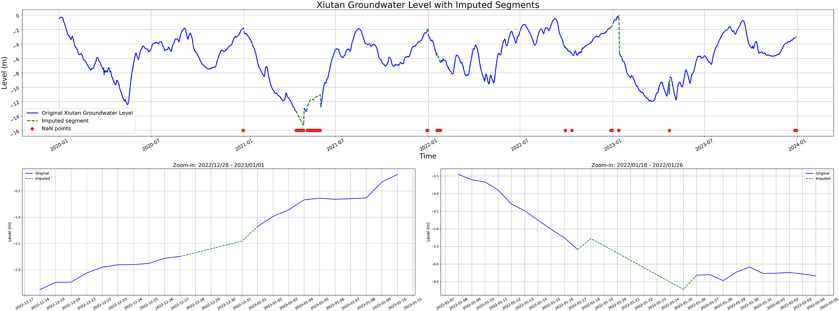
Figure 2: Groundwater water level imputation results at Xiutan (2020–2023). Enlarged views of two imputation segments are shown below

To further examine the effectiveness of the imputation method in preserving data trends, two imputed segments were selected for zoom-in visualization to assess the continuity between the imputed values and their surrounding data. The zoomed-in views reveal that the imputed data align well with the original observations in terms of continuity and trend transitions, with no apparent structural discontinuities, abnormal deviations, or unrealistic fluctuations. These results indicate that the imputation process adopted in this study demonstrates good smoothness and trend-preservation capabilities, thereby contributing to the quality and stability of input data for subsequent prediction models.

4.3 Groundwater Level Prediction Results

4.3.1 Hyperparameter Optimization Results

The use of Bayesian optimization enabled systematic and efficient hyperparameter tuning, which helps avoid suboptimal configurations and improves model robustness without the need for exhaustive manual searching. Based on the hyperparameter search space defined in Section 3.3.3, a total of 360 hyperparameter combinations were tested using Bayesian Optimization. Optimal hyperparameters were determined for BiLSTM, LSTM, and RNN through the tuning process. A summary of these configurations is presented in Table 2.

During the training process, all models were trained with a fixed batch size of 16, using MSE as the loss function and the Adam optimizer to balance stability and convergence speed. Each training run was set to a maximum of 100 epochs, with early stopping applied (patience set to 10) to prevent overfitting. As for the dataset, this study utilized daily groundwater and river water level observations from 2020 to 2023, comprising a total of 1461 records. The data were split chronologically into 80% for training, 10% for validation, and 10% for testing.

4.3.2 Model Prediction Results

This section presents the groundwater level prediction results produced by the BiLSTM, LSTM, and RNN models. Each model was independently trained and tested ten times, and the average performance was reported to mitigate the effects of randomness. The predictive performance across the ten repeated runs for each model is summarized in Table 3.

The Table 3 reports the R2 and MSE scores for each run, allowing further assessment of prediction accuracy and consistency. Overall, the BiLSTM model exhibited higher and more stable R2 values along with lower MSE scores, indicating superior trend fitting and error control capabilities. In contrast, the LSTM and RNN models showed greater variability in performance across different runs. In the subsequent analysis, line plots are used to illustrate the comparison of actual groundwater level changes and model predictions, while box plots are employed to compare the distribution of R2 and MSE scores across models, providing a more comprehensive evaluation of their accuracy and stability.

Figs. 3 and 4 illustrate the prediction performance of BiLSTM, LSTM, and RNN models on test data from August to December 2023, including trend plots and linear regression analyses. Fig. 3a–c shows the average predictions (blue lines) from ten independent training runs for three different models, overlaid with actual groundwater levels (black lines), highlighting each model’s ability to capture time-series trends. Fig. 4a–c presents the corresponding linear regression results between predicted and observed values, used to assess prediction accuracy and overall fit.

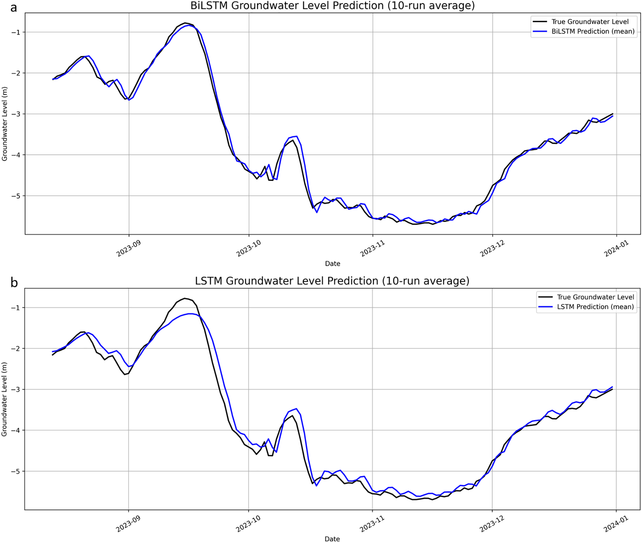
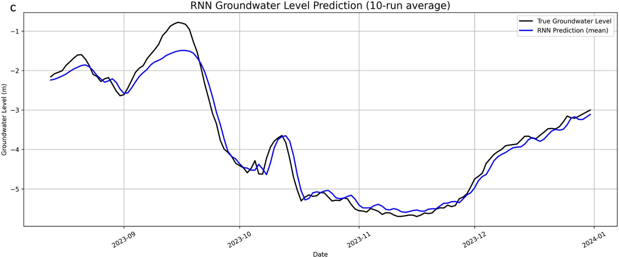
Figure 3: Predicted groundwater level time series using BiLSTM, LSTM, and RNN models. (a): BiLSTM Groundwater Level Prediction (10-run average). (b): LSTM Groundwater Level Prediction (10-run average). (c): RNN Groundwater Level Prediction (10-run average)

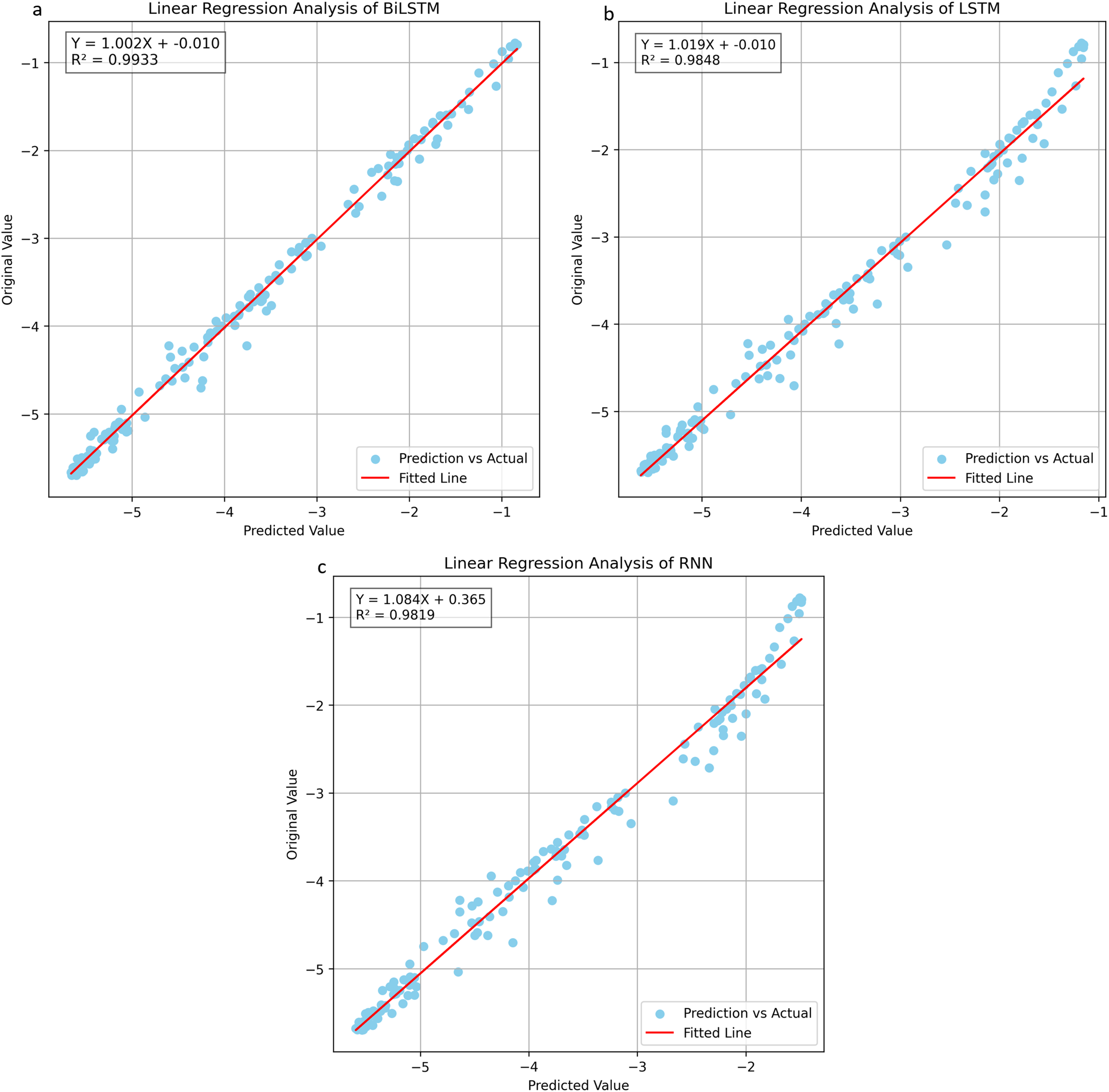
Figure 4: Comparative linear regression plots for BiLSTM, LSTM, and RNN models. (a): Linear regression analysis of BiLSTM. (b): Linear regression analysis of LSTM. (c): Linear regression analysis of RNN

The regression results align with these observations. BiLSTM achieves the best linear fit, with a slope closest to 1, the smallest intercept, and the highest R2 (0.9933), indicating excellent agreement with observed data. LSTM and RNN also show strong correlations, with slightly lower R2 values of 0.9848 and 0.9819, respectively, and larger deviations in slope and intercept.

In response to the need for a more comprehensive evaluation, we further computed additional evaluation metrics based on the mean predictions across 10 training runs. Table 4 summarizes the R2, MSE, RMSE, MAE, and MAPE values for BiLSTM, LSTM, and RNN models. As shown in the table, BiLSTM achieved the lowest errors across all metrics, including a MAPE of only 3.14%, demonstrating its superior accuracy and robustness in groundwater level forecasting.

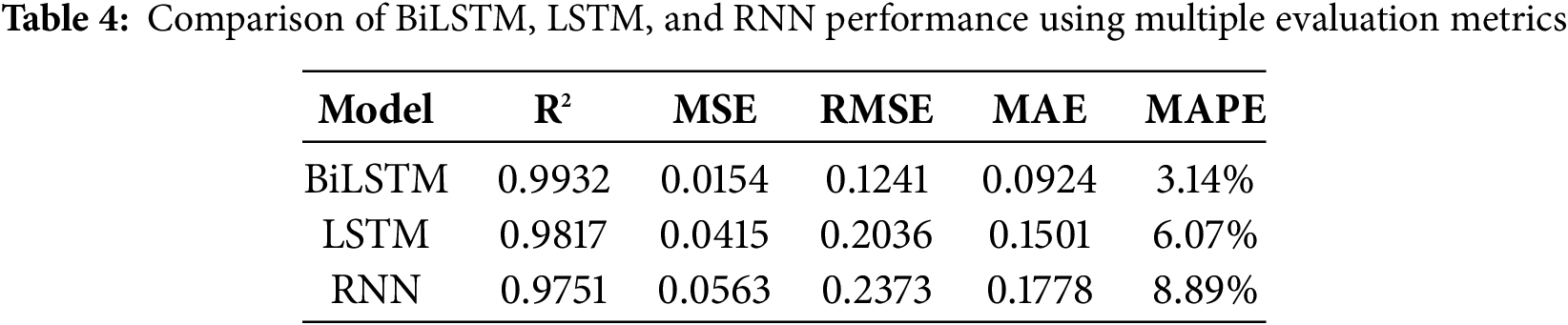
Fig. 5 respectively present box plot comparisons of the R2 and MSE metrics across ten prediction runs for the BiLSTM, LSTM, and RNN models, illustrating the prediction accuracy and stability of each model. As shown in Fig. 5a, the BiLSTM model demonstrates a highly concentrated distribution of R2 scores, with an extremely narrow interquartile range (IQR), indicating that all training runs consistently achieved a high accuracy of approximately 0.993. In contrast, both the LSTM and RNN models exhibit greater variability, with the RNN model showing noticeably lower median and mean R2 values compared to the other models, reflecting its overall weaker prediction accuracy. As shown in Fig. 5b, the BiLSTM model not only achieved the lowest average error in terms of MSE but also exhibited the smallest variability, further confirming its superior stability. In contrast, the LSTM model showed slightly higher errors, while the RNN model demonstrated a broader error range, with some training runs resulting in significantly larger prediction errors.

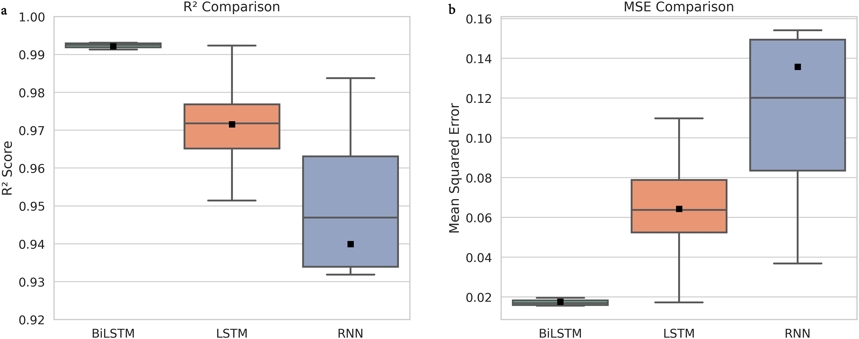
Figure 5: Accuracy and error metrics comparison for BiLSTM, LSTM, and RNN forecasting models. (a): Comparison of R2 scores for the BiLSTM, LSTM, and RNN models. (b): Comparison of MSE among the BiLSTM, LSTM, and RNN models

This advantage may stem from the model’s ability to process input sequences in both forward and backward directions, allowing it to capture information from surrounding time steps. This capability is particularly valuable in hydrological systems characterized by delayed responses, such as the hysteresis effect between river and groundwater levels.

Overall, the BiLSTM model significantly outperformed both the LSTM and RNN models in terms of prediction accuracy and error control, highlighting its superior performance in learning and forecasting complex groundwater level variations. This study also compared its findings with relevant regional applications. Ghasemlounia et al. [26] applied a BiLSTM model to predict groundwater levels at four observation wells in the Miandoab plain, West Azerbaijan Province, Iran, achieving R2 values ranging from approximately 0.75 to 0.89, with a best-case result of R2 = 0.89. Vu et al. [8] conducted river and groundwater level forecasting in Normandy, western France, reporting relative errors between 3% and 5%, demonstrating good stability and applicability. In comparison, this study achieved an average R2 of 0.9932 and an MSE of 0.0154 in the Zhuoshui River alluvial fan area in Taiwan, along with a mean absolute percentage error (MAPE) of 3.14%. These results indicate enhanced predictive performance and robust error control compared to previous studies, suggesting that the proposed system has strong potential for generalization across regions.

5  Conclusion

5.1 Data Prediction Results

This study proposed an integrated groundwater level forecasting system that combines a cloud-based data management framework with deep learning models. Through the integration of imputation methods and multiple model training strategies, the system is designed to improve predictive reliability and maintain stable performance in forecasting groundwater level dynamics. The proposed framework utilizes STL in conjunction with the SARIMA model for anomaly-aware data imputation and employs three regression models, including BiLSTM, LSTM, and RNN, trained and evaluated using sensor data collected from 2020 to 2023. Centered on Taiwan’s Zhuoshui River alluvial fan, this research aims to predict groundwater level variations within a three-month forecasting window.

Experimental results indicate that river water levels have strong predictive power for groundwater level changes. Among the models, BiLSTM consistently achieved the best performance in terms of R2 and MSE, demonstrating superior generalization ability and prediction stability. The data imputation mechanism effectively mitigated the impact of sensor anomalies on model training and forecasting, thereby further improving overall performance. The system successfully integrates data acquisition, preprocessing, model training, and result analysis, showcasing its potential as a real-time and scalable groundwater forecasting solution within a cloud-based architecture.

It is important to note that the proposed system assumes the use of two monitoring stations with a strong correlation and continuous daily monitoring data (despite some missing values). The model’s effectiveness in regions with sparse sensor coverage or lower data frequency remains to be evaluated further and represents a crucial direction for future research and practical deployment.

5.2 Limitations and Future Works

The current study presents several limitations and opportunities for future improvement.

First, although river and groundwater monitoring stations with upstream–downstream relationships were used, the effects of spatial distance and flow lag were not explicitly modeled. Future work could incorporate these delay effects into feature engineering to evaluate their impact on predictive performance from both physical and statistical perspectives.

Second, due to the absence of ground truth in missing data segments, the imputation results could not be evaluated using conventional error metrics. Therefore, this study relied on trend consistency and visual inspection. Future research could simulate missing patterns to enable quantitative validation, and also benchmark the STL-SARIMA approach against alternative methods such as linear interpolation and KNN interpolation.

Third, model evaluation was limited to the Zhuoshui River alluvial fan region. Future studies should assess cross-regional applicability by applying the model to areas with diverse hydrogeological and climatic conditions.

Additionally, this study focused on predictions within a 3-month window. Future research should evaluate performance over longer time horizons (e.g., 6–12 months) and examine seasonal variation, particularly between wet and dry periods, to better understand the model’s robustness under varying hydrological conditions.

Lastly, to improve model interpretability and transparency, future work will explore the use of SHAP (SHapley Additive exPlanations) values and attention mechanisms to quantify the contributions of input features to prediction outcomes.

Acknowledgement: Not applicable.

Funding Statement: This research was funded by the Taiwan Comprehensive University System and the National Science and Technology Council of Taiwan under grant number NSTC 111-2410-H-019-006-MY3 and NSTC 114-2410-H-194-019-MY2. Additionally, this work was financially/partially supported by the Advanced Institute of Manufacturing with High-tech Innovations (AIM-HI) from the Featured Areas Research Center Program within the framework of the Higher Education Sprout Project by the Ministry of Education (MOE) in Taiwan.

Author Contributions: The authors confirm contribution to the paper as follows: data collection: Yun-Chin Wu, Zheng-Yun Xiao and Ting-Jou Ding; draft manuscript preparation: Yu-Sheng Su and Yi-Wen Wang. All authors reviewed the results and approved the final version of the manuscript.

Availability of Data and Materials: The data that support the findings of this study are available from the corresponding author, Yu-Sheng Su, upon reasonable request.

Ethics Approval: Not applicable.

Conflicts of Interest: The authors declare no conflicts of interest to report regarding the present study.

References

1. Ohenhen LO, Zhai G, Lucy J, Werth S, Carlson G, Khorrami M, et al. Land subsidence risk to infrastructure in US metropolises. Nat Cities. 2025;1(6):1–12. doi:10.1038/s44284-025-00240-y. [Google Scholar] [CrossRef]

2. Al-Ozeer AZ, Al-Abadi AM, Hussain TA, Fryar AE, Pradhan B, Alamri A, et al. Modeling of groundwater potential using cloud computing platform: a case study from Nineveh Plain, Northern Iraq. Water. 2021;13(23):3330. doi:10.3390/w13233330. [Google Scholar] [CrossRef]

3. Lu CY, Hu JC, Chan YC, Su YF, Chang CH. The relationship between surface displacement and groundwater level change and its hydrogeological implications in an alluvial fan: case study of the Choshui River. Taiwan Remote Sens. 2020;12(20):3315. doi:10.3390/rs12203315. [Google Scholar] [CrossRef]

4. Sherstinsky A. Fundamentals of recurrent neural network (RNN) and long short-term memory (LSTM) network. Physica D. 2020;404(8):132306. doi:10.1016/j.physd.2019.132306. [Google Scholar] [CrossRef]

5. Satishkumar U, Kulkarni P. Simulation of groundwater level using recurrent neural network (RNN) in Raichur District, Karnataka. India Int J Curr Microbiol Appl Sci. 2018;7(12):3358–67. doi:10.20546/ijcmas.2018.712.387. [Google Scholar] [CrossRef]

6. Solgi R, Loaiciga HA, Kram M. Long short-term memory neural network (LSTM-NN) for aquifer level time series forecasting using in-situ piezometric observations. J Hydrol. 2021;601(8):126800. doi:10.1016/j.jhydrol.2021.126800. [Google Scholar] [CrossRef]

7. Siami-Namini S, Tavakoli N, Namin AS. The performance of LSTM and BiLSTM in forecasting time series. In: Proceedings of the 2019 IEEE International Conference on Big Data (Big Data); 2019 Dec 9–12; Los Angeles, CA, USA. doi:10.1109/BigData47090.2019.9005997. [Google Scholar] [CrossRef]

8. Vu MT, Jardani A, Massei N, Deloffre J, Fournier M, Laignel B. Long-run forecasting surface and groundwater dynamics from intermittent observation data: an evaluation for 50 years. Sci Total Environ. 2023;880(4):163338. doi:10.1016/j.scitotenv.2023.163338. [Google Scholar] [PubMed] [CrossRef]

9. Su YS, Hu YC, Wu YC, Lo CT. Evaluating the impact of pumping on groundwater level prediction in the Chuoshui River alluvial fan using artificial intelligence techniques. Int J Interact Multimed Artif Intell. 2024;8(7):28–37. doi:10.9781/ijimai.2024.04.002. [Google Scholar] [CrossRef]

10. Blázquez-García A, Conde A, Mori U, Lozano JA. A review on outlier/anomaly detection in time series data. ACM Comput Surv. 2021;54(3):1–33. doi:10.1145/3444690. [Google Scholar] [CrossRef]

11. Grubbs FE. Procedures for detecting outlying observations in samples. Technometrics. 1969;11(1):1–21. doi:10.2307/1266761. [Google Scholar] [CrossRef]

12. Valipour M. Long-term runoff study using SARIMA and ARIMA models in the United States. Meteorol Appl. 2015;22(3):592–8. doi:10.1002/met.1491. [Google Scholar] [CrossRef]

13. Lee S, Kim HK. ADSaS: comprehensive real-time anomaly detection system. Lect Notes Comput Sci. 2019;11539(1):29–41. doi:10.1007/978-3-030-17982-3_3. [Google Scholar] [CrossRef]

14. Tejada AJr, Talento MS, Ebal LP, Villar C, Dinglasan BL. Forecasting of monthly closing water level of Angat Dam in the Philippines: SARIMA modeling approach. J Environ Sci Manag. 2023;26(2):42–51. doi:10.47125/jesam/2023_2/04. [Google Scholar] [CrossRef]

15. Adamowski J, Chan HF, Prasher SO, Shamseldin AY, Ishak SZ. Comparison of multiple linear and nonlinear regression, autoregressive integrated moving average, artificial neural network, and wavelet-artificial neural network models for urban water demand forecasting in Montreal. Canada Water Resour Res. 2012;48(1):w01528. doi:10.1029/2010WR009945. [Google Scholar] [CrossRef]

16. Kombo OH, Kumaran S, Bovim A. Design and application of a low-cost, low-power, LoRa-GSM, IoT enabled system for monitoring of groundwater resources with energy harvesting integration. IEEE Access. 2021;9:128417–33. doi:10.1109/ACCESS.2021.3112519. [Google Scholar] [CrossRef]

17. Hinton GE, Osindero S, Teh YW. A fast learning algorithm for deep belief nets. Neural Comput. 2006;18(7):1527–54. doi:10.1162/neco.2006.18.7.1527. [Google Scholar] [PubMed] [CrossRef]

18. Le XH, Ho HV, Lee G, Jung S. Application of long short-term memory (LSTM) neural network for flood forecasting. Water. 2019;11(7):1387. doi:10.3390/w11071387. [Google Scholar] [CrossRef]

19. Bengio Y, Simard P, Frasconi P. Learning long-term dependencies with gradient descent is difficult. IEEE Trans Neural Netw. 1994;5(2):157–66. doi:10.1109/72.279181. [Google Scholar] [PubMed] [CrossRef]

20. Hochreiter S, Schmidhuber J. Long short-term memory. Neural Comput. 1997;9(1):1–42. doi:10.1162/neco.1997.9.1.1. [Google Scholar] [CrossRef]

21. Gers FA, Schmidhuber J, Cummins F. Learning to forget: continual prediction with LSTM. Neural Comput. 2000;12(10):2451–71. doi:10.1162/089976600300015015. [Google Scholar] [PubMed] [CrossRef]

22. Zhang J, Zhu Y, Zhang X, Ye M, Yang J. Developing a long short-term memory (LSTM) based model for predicting water table depth in agricultural areas. J Hydrol. 2018;561(53):918–29. doi:10.1016/j.jhydrol.2018.04.065. [Google Scholar] [CrossRef]

23. Patra SR, Chu HJ. Convolutional long short-term memory neural network for groundwater change prediction. Front Water. 2024;6:1471258. doi:10.3389/frwa.2024.1471258. [Google Scholar] [CrossRef]

24. Baziotis C, Pelekis N, Doulkeridis C. DataStories at SemEval-2017 Task 4: deep LSTM with attention for message-level and topic-based sentiment analysis. In: Proceedings of the 11th International Workshop on Semantic Evaluation (SemEval-2017); 2017 Aug 3–4; Vancouver, BC, Canada. [Google Scholar]

25. Ali ASA, Jazaei F, Babakhani P, Ashiq MM, Bakhshaee A, Waldron B. An overview of deep learning applications in groundwater level modeling: bridging the gap between academic research and industry applications. Appl Comput Intell Soft Comput. 2024;2024(1):9480522. doi:10.1155/2024/9480522. [Google Scholar] [CrossRef]

26. Ghasemlounia R, Gharehbaghi A, Ahmadi F, Saadatnejadgharahassanlou H. Developing a novel framework for forecasting groundwater level fluctuations using Bi-directional long short-term memory (BiLSTM) deep neural network. Comput Electron Agric. 2021;191(12):106568. doi:10.1016/j.compag.2021.106568. [Google Scholar] [CrossRef]

27. Su YS, Hu YC. Applying cloud computing and Internet of Things technologies to develop a hydrological and subsidence monitoring platform. Sensors Mater. 2022;34(4):1313–21. doi:10.18494/SAM3508. [Google Scholar] [CrossRef]

28. Chang T, Wang K, Wang S, Hsu C, Hsu C. Evaluation of the groundwater and irrigation quality in the Zhuoshui River alluvial fan between wet and dry seasons. Water. 2022;14(9):1494. doi:10.3390/w14091494. [Google Scholar] [CrossRef]

29. Hutter F, Kotthoff L, Vanschoren J. The Springer series on challenges in machine learning [Internet]. Cham, Switzerland: Springer; 2024 [cited 2024 Jan 1]. Available from: https://library.oapen.org/bitstream/handle/20.500.12657/23012/1007149.pdf. [Google Scholar]

30. Andonie R. Hyperparameter optimization in learning systems. J Membr Comput. 2019;1(4):279–91. doi:10.1007/s41965-019-00023-0. [Google Scholar] [CrossRef]

31. Roy K. Tutorial—Shodhguru Labs: optimization and hyperparameter tuning for neural networks [Internet]. Columbia, SC, USA: University of South Carolina; 2023 [cited 2024 Jan 1]. Available from: https://scholarcommons.sc.edu/aii_fac_pub/584. [Google Scholar]

32. Khan J, Lee E, Balobaid AS, Kim K. A comprehensive review of conventional, machine learning, and deep learning models for groundwater level (GWL) forecasting. Appl Sci. 2023;13(4):2743. doi:10.3390/app13042743. [Google Scholar] [CrossRef]