Advanced Multi-Channel Echo Separation Techniques for High-Interference Automotive Radars

1  Introduction

As the demand for autonomous driving and advanced driver assistance systems (ADAS) continues to rise, automotive radars must maintain stable and highly accurate detection capabilities even under noisy and interference-prone real-world conditions. In recent years, multichannel radars and sensor fusion have emerged as key research topics, as they can simultaneously reduce clutter and interference while enhancing target identification, particularly in complex multi-vehicle scenarios, urban environments with significant reflections, and multi-radar networking. By employing diverse antenna configurations, multi-beam approaches, and cooperative computation, researchers are progressively addressing challenges such as interference suppression, channel estimation, and sensor data integration, thereby fostering a more robust and safer intelligent vehicle environment.

Kronauge and Rohling [1] propose new chirp sequence waveforms that enhance range and Doppler resolution in automotive radar systems. Venon et al. [2] deliver a comprehensive survey on mmWave FMCW radars for perception, recognition, and localization, highlighting their significance in modern vehicles. Rameez et al. [3] address interference compression and mitigation challenges, whereas Haider et al. [4] elaborate on modeling and simulation frameworks to support robust environmental perception. Wang et al. [5] employ contrastive learning with dilated convolution to combat radar interference, and Wang et al. [6] introduce time and frequency domain decomposition for mutual interference. Sun et al. [7] develop a millimeter-wave radar with high angular resolution to detect closely spaced road obstacles. Alland et al. [8] review interference characteristics, mitigation methods, and future research avenues. Hakobyan and Yang [9] examine high-performance signal processing algorithms and modulation schemes, and Nikandish et al. [10] discuss the emergence of spurs in millimeter-wave radar systems. Yan and Roberts [11] focus on recent advancements in millimeter-wave technologies, emphasizing signal processing perspectives. Doris et al. [12] reframe fast-chirp FMCW transceivers to realize superior resolution, and Arai et al. [13] demonstrate a 77-GHz 8RX3TX transceiver fabricated in 40-nm CMOS. Lastly, Caffa et al. [14] showcase the integration of a 77-GHz automotive radar into a car’s rear lamp, underscoring the potential for compact and efficient designs. Eder and Eldar [15] propose a sparsity-based method for multi-person, non-contact vital signs monitoring via FMCW radar. Next, Gupta et al. [16] employ machine learning on range-angle images to enable accurate target classification using mmWave radars. Lastly, Shamsfakhr et al. [17] introduce a multi-target detection and tracking algorithm leveraging mmWave-FMCW radar data.

Hyvärinen and Oja [18] present fundamental ICA algorithms and their practical applications, underscoring the technique’s power in blind source separation. Tharwat [19] provides an extensive overview of ICA, detailing its theoretical foundations and real-world benefits. Building on these concepts, Mehta et al. [20] integrate topographic ICA with 3D Convolution Neural Networks (CNNs) for predicting material properties from microstructure images. Meanwhile, Engel et al. [21] propose a kernel-based RLS algorithm to handle nonlinear scenarios more effectively. Benesty et al. [22] delve into advanced RLS methodologies for acoustic echo cancellation, and Paleologu et al. [23] introduce data-reuse techniques that enhance RLS convergence performance.

Huang et al. [24] introduce empirical mode decomposition (EMD) and the Hilbert spectrum for dissecting nonlinear, non-stationary signals, providing a foundational approach to time-frequency analysis. Subsequently, Huang et al. [25] further demonstrate EMD’s capability to reveal complex wave behaviors, particularly in fluid mechanics. Wu and Huang [26] expand this methodology by proposing ensemble EMD (EEMD), which employs noise assistance to mitigate mode mixing and improve decomposition stability. Meanwhile, Randall and Antoni [27] question EMD’s practical benefits for bearing diagnostics, highlighting limitations in industrial contexts. Collectively, these works underscore EMD’s potential and controversies for real-world signal processing.

Dragomiretskiy and Zosso [28] propose VMD as a robust approach to decomposing nonlinear, nonstationary signals, mitigating the mode-mixing challenges often encountered in EMD. Building on this, ur Rehman and Aftab [29] extend VMD to handle multivariate datasets, accommodating broader real-world applications. Nazari and Sakhaei [30] streamline the decomposition process by introducing successive VMD. Moreno et al. [31] combine VMD with singular spectral analysis and machine learning to enhance wind speed forecasting accuracy. Gu et al. [32] adopt VMD, continuous wavelet transform, and an improved CNN to diagnose rotating machinery faults. Hadiyoso et al. [33] compare EMD, VMD, and EEMD methods in respiration wave extraction, whereas Chen et al. [34] harness both EMD and VMD in deep learning for radio modulation recognition. Seyrek et al. [35] evaluate these decompositions for chatter detection in milling, and Yun and Jian [36] propose a parameter-selection strategy to avoid modal overlap. Zhao et al. [37] incorporate VMD-EEMD and self-attention mechanisms for weak signal detection in chaotic noise.

Lin et al. [38] integrate ICA with EMD to enhance data analysis in complex signals. Continuing this direction, Lin et al. [39] employ ICA-EEMD in chaotic systems for secure communications. Lin [40] combines variational mode decomposition (VMD) with ResNet101, demonstrating an intelligent motor fault diagnosis scheme. In another work, Lin [41] applies EMD techniques to improve deep learning performance in U.S. GDP forecasting. Lin [42] also presents an ICA-VMD method to bolster diagnostic accuracy in low signal-to-noise ratio settings.

Von Kügelgen et al. [43] validate that self-supervised learning strategies can effectively disentangle content and style. Geirhos et al. [44] investigates shortcut learning, highlighting vulnerabilities in deep neural networks. Farahani et al. [45] systematically review graph-theoretic analyses for detecting connectivity patterns within human brain networks. Finally, Alibakhshi-Kenari et al. [46] employed composite transmission-line techniques to realise an ultra-wideband microstrip antenna that combines size reduction with broad impedance bandwidth; they [47] later adopted a CRLH configuration to achieve an even smaller footprint while maintaining high radiation efficiency.

This study introduces a multi-channel signal processing framework tailored for dual FMCW radars operating in high-noise scenarios. The proposed method significantly enhances target range estimation accuracy by integrating an enhanced ICA-based adaptive filtering technique with VMD and the HHT. Simulation results reveal that effective echo separation, noise suppression, and beat-frequency extraction collectively contribute to superior detection performance. This demonstrates the method’s potential for robust target ranging under challenging interference conditions.

2  Description of the Research Methodology

2.1 FMCW Radar Theoretical

Frequency-Modulated Continuous-Wave (FMCW) radar typically employs a linear frequency modulation (LFM) [1–3] chirp as its transmitted signal, which can be expressed as:

s(t)=Acos⁡[2π(f1t+12αt2)],(1)

where A is the transmit amplitude. The starting frequency of the sweep is f1, and the chirp slope α is defined by:

α=f2−f1T,(2)

with T being the duration of one frequency sweep. If the frequency ramps from f2=f1+Δf by the end of the sweep, then:

Δf=f2−f1=αT(3)

For the single-target scenario, consider a target located at distance R. An electromagnetic wave traveling at the speed of light ccc experiences a round-trip delay.

If the frequency ramps from:

τ=2Rc.(4)

Without noise or other perturbations, the received echo is ideally given by:

xecho(t)=Arcos⁡[2π(f1(t−τ)+12α(t−τ)2)],(5)

where Ar is the echo amplitude, which depends on the target’s radar cross section (RCS), antenna gains, etc.

A fundamental principle of FMCW radar relies on the beat frequency fb, generated by mixing (multiplying) the transmitted chirp s(t) with the delayed echo xecho(t). Under ideal conditions, the resulting beat frequency approximates.

fb≈ατ=ΔfT⋅2Rc(6)

From this, the distance can be estimated by:

Rb=cT2ΔfTfb,(7)

where Δf=f2−f1. In practical implementations, performing a Fast Fourier Transform (FFT) on the mixed signal to locate the peak corresponding to fb enables straightforward range estimation of the target. Eqs. (1)–(7) follow directly from the standard FMCW range-equation derivation in the radar literature [48,49].

2.2 Proposed Enhanced Independent Component Analysis for Two Automotive Radar Echoes

In practical automotive radar systems, two radar echoes x1 and x2 are frequently contaminated by interference and environmental noise, forming a multi-channel signal mixture. Let:

x(t)=[x1x2],(8)

represent these two measurement channels. Suppose these channels derive from two independent source signals, such as the desired target echo and various interference components. Directly assumes statistical independence of sources; see Hyvärinen & Oja [18]. The overall mixed model can be written as:

x(t)=As(t)+n(t)(9)

where A is an unknown mixing matrix of size 2 × 2, s (t)∈R2 is the vector of independent sources (including the ideal echo), and n(t) represents additional noise.

Independent Component Analysis (ICA) [18,19] seeks to estimate a demixing matrix W≈A−1 under the assumption that the source signals are statistically independent. Follows from the maximum-likelihood solution in FastICA [50]. By applying:

y(t)=Wx(t)(10)

we recover each independent component s(t) (up to scaling and permutation). A common way to measure non-Gaussianity in ICA is via negentropy or kurtosis. The non-Gaussianity measure, introduced by Hyvärinen and Oja [18], is widely used in Blind Source Separation (BSS), as also noted in tutorial notes on ICA statistics [50,51]. For instance, let y=wTx(t). The kurtosis κ(y) is defined as:

κ(y)=E[y4]−3(E[y2])2(11)

If κ(y)≠0, y is deemed non-Gaussian; a purely Gaussian distribution would yield κ=0. Derived by maximizing negentropy; see Hyvärinen’s original FastICA paper [50,51]. A typical FastICA update rule for extracting a single component is:

wnew=E[xg(wTx)]−E[g′(wTx)]w,(12)

where g(⋅) is a nonlinear function (e.g., tanh⁡(⋅)) and g′(⋅) its derivative. After normalizing ∥wnew∥ = 1 and iterating until convergence, the algorithm obtains one demixing vector. Repeating this process alongside orthogonalization or whitening steps allows extraction of multiple independent components, forming W=[w1,w2,…].

In our approach, ICA provides a 2 × 2 demixing matrix W. Immediately from multiplying W by the data matrix X; also used in Cardoso’s Joint Approximate Diagonalization of Eigen-matrices (JADE) implementation [52]. Multiplying W by the two-channel data X yields.

U=WX(13)

Although one of the separated components typically approximates the target echo, it may still suffer from amplitude scaling or residual noise. Therefore, we further employ RLS-based calibration to correct channel mismatches and suppress interference. This enhanced methodology effectively addresses two-channel echo signals, improving the robustness of target detection in automotive radar applications.

2.3 RLS Adaptive Filtering Calibration

Although ICA can separate independent sources, variations in radar channel characteristics, such as amplitude and phase mismatches, often leave the separated echo signal deviating from the original measurements. To compensate for these discrepancies, this work employs an RLS adaptive filter.

RLS Update Eqs. (21)–(23): Let:

u(n)=[xunmix,1(n)xunmix,2(n)],d(n)=x1(n)(14)

where d(n) denotes the desired output (corresponding to the actual radar measurement). The RLS algorithm proceeds iteratively as follows:

I. Kalman Gain

k(n)=P(n−1)u(n)λ+uT(n)P(n−1)u(n),(15)

where 0 < λ ≤ 1 is the forgetting factor.

II. Prediction Error

e(n)=d(n)−wT(n−1)u(n).(16)

III. Weight Update

w(n)=w(n−1)+k(n)e(n)(17)

IV. P Update

P(n)=1λ[P(n−1)−k(n)uT(n)P(n−1)].(18)

Once convergence is reached, the final calibrated echo is formed by

xunmixed_rls(n)=wTu(n),(19)

which is expected to closely approximate the true radar echo.

2.4 VMD/HHT Analysis

To gain a deeper understanding of, and to further eliminate residual noise, the calibrated signal xunmixed_rls is processed via VMD [28–30]. The signal is decomposed into several intrinsic mode functions (IMFs) as

xunmixed_rls(t)=∑k=1Kuk(t)(20)

VMD resembles EMD, yet adopts a variational method in the frequency domain to ensure non-overlapping mode bandwidths, thereby enhancing numerical stability.

Each IMF is then subjected to a Hilbert transform to obtain instantaneous frequency, forming the HHT in time-frequency space. This step reveals the primary components carried by each mode. At this stage, the user may discard noise-dominated IMFs or selectively combine the most relevant IMFs to reconstruct a relatively clean target signal.

2.5 Distance Estimation from Combined IMFs

Finally, summing the selected IMFs yields a “denoised” signal xrecon(t). Prior to the FFT, a Hann window and 10× zero-padding are applied to reduce spectral leakage and improve frequency resolution [49]. Multiplying it by the transmitted chirp s(t) (corresponding to FMCW mixing) in the frequency domain exposes the beat frequency f^b. Practically, we compute:

xmix(t)=s(t)⋅xrecon(t)(21)

then take the FFT of xmix to locate the dominant peak at f^b. Substituting f^b into:

Rest=cT2(f2−f1)f^b(22)

yields the estimated target distance. When f^b closely matches the theoretical value, it indicates that the overall process—encompassing dual-channel radar mixture, ICA separation, RLS calibration, and VMD/HHT noise suppression—effectively mitigates external interference. A deviation in our Monte-Carlo tests confirms that this enhanced ICA and VMD/HHT scheme chain effectively removes interference and restores the beat tone.

3  Research Design and Setup

In this study, a 10-s synthetic signal was first generated to validate the performance of the enhanced VMD. The sampling frequency, fs, was set to 100 Hz, providing 1000 data points across the 0–10 s interval. Three target sine waves at 5, 15, and 25 Hz were constructed, defined respectively as:

s1=sin⁡(2π⋅5t),s2=sin⁡(2π⋅15t),s3=sin⁡(2π⋅25t)(23)

To emulate practical measurement conditions, random noise n with a zero-mean distribution was added, yielding the final composite signal.

x(t)=s1(t)+s2(t)+s3+n(t).(24)

By computing and comparing the average energies of the signal and noise, an SNR value of 12.7221 dB was obtained in this setup. Adjusting the noise energy thus allows for various signal-to-noise ratio scenarios, enabling a clearer observation of how noise influences the overall signal behavior. Through this synthetic signal and adjustable noise framework, the subsequent analysis examines how effectively the enhanced VMD can separate multi-frequency components and suppress noise across different disturbance scenarios.

In the proposed enhanced VMD algorithm, the number of decomposition modes is set to five, ensuring that the three target frequency components can be properly extracted along with any potential noise or residual components. To govern each mode’s average bandwidth, a frequency band suppression parameter is introduced, whose value is set to 60,000; increasing this parameter strengthens the suppression of high-frequency elements, although it may reduce the overall resolution during decomposition. The value is temporarily assigned to zero for dual ascent time steps to maintain flexibility (and can be omitted if unnecessary). To better account for the original signal’s coherency, the enhanced VMD’s energy function includes a data coupling weight fixed at 70; higher values strengthen the emphasis on the original signal and, consequently, increase the absorption of noise. Lastly, the convergence tolerance is set to 10−5, and the algorithm terminates as soon as the quantitative change between consecutive iterations falls below this threshold, thus ensuring the stability and efficiency of the iterative process. All numerical experiments were conducted in MATLAB R2015a (MathWorks, Natick, MA, USA) using built-in Signal Processing and Wavelet toolboxes.

4  Results and Discussion

As shown in Fig. 1, panel (A) depicts the first base-band channel returned by Radar-1: it consists of the ideal 50 m echo plus zero-mean white Gaussian noise. Panel (B) shows the second channel recorded by Radar-2. The time-domain signals received by two automotive radars under numerical simulation over the sampling period of 0–1 s. Both signals are notably covered by random white noise, with amplitudes spanning approximately ±2 and a near-zero mean, indicating comparable noise energy levels. Due to the relatively weak amplitude of the echo signals, the target features are completely masked by noise, rendering direct extraction of the time-domain echo components impossible.

Figure 1: Simulated base-band signals acquired by two automotive radars: (A) Radar 1, 50 m target echo superimposed on zero-mean white Gaussian noise; (B) Radar 2, corresponding channel under identical noise conditions

Fig. 2A presents one of the independent components obtained via standard ICA separation. Its amplitude range is relatively small, approximately within ±0.05, indicating that ICA has automatically scaled down this component’s amplitude. Compared with the original echo or external noise, certain structural elements remain discernible; however, it is not immediately clear whether this signal represents the primary echo. A quick energy analysis shows that this component carries only ~2% of the total signal power, implying it is the weak echo buried in noise. Its low power necessitates the later denoising stages to reveal the beat tone. In contrast, the signal in Fig. 2B exhibits an amplitude range of about ±2, closely resembling noise. This suggests that the other component likely contains most of the noise energy, although some portion of the echo may still be mixed in. Although traditional ICA theoretically separates statistically independent sources, in practical radar or noisy environments, imperfections due to channel gain disparities and nonlinear interference may prevent a clean delineation into purely “echo” or purely “noise.”

Figure 2: Independent components extracted by the conventional ICA algorithm: (A) low-amplitude component (∼±0.05) carrying ≈2% of the total power—weak echo masked by noise; (B) high amplitude component (∼±2) dominated by noise, with residual echo still mixed in

In Fig. 3, five IMFs are shown in distinct colours, each representing a separate frequency band obtained by the VMD algorithm. From bottom to top, the centre frequency increases, evidenced by the slight upward “tilt” of the coloured traces across time. The blue IMF (Mode 1) retains the slow-varying chirp component that later produces the beat tone, whereas the green IMF (Mode 5) is dominated by high-frequency residual noise.

Figure 3: VMD-based analysis of signal (A) from Fig. 2 obtained using the conventional ICA algorithm

Fig. 4 shows the time-frequency map obtained by applying the Hilbert-Huang transform to the five VMD modes in Fig. 3. Here, the vertical axis is frequency (0–5 kHz), the horizontal axis is time (0–1 s), and the colour bar (×10−4) represents instantaneous energy. Three nearly horizontal “bands” centred at ≈1, 2, and 4 kHz (green-yellow streaks) correspond to the chirp’s first three harmonics that carry the target echo. Their continuity over time indicates a stable beat pattern. The faint vertical stripes and diffuse blue areas are residual broadband noise and mode-mixing artefacts. By thresholding on the high-energy bands (green/yellow), we can isolate the predictable echo components while suppressing the scattered low-energy regions that stem from noise.

Figure 4: HHT-based analysis (after VMD) of signal (A) from Fig. 3 obtained using the conventional ICA algorithm

From Fig. 5A, it is evident that the enhanced ICA approach effectively suppresses most of the noise components in the mixed signal, confining the echo amplitude largely within ±1 and thus yielding a time-domain profile closer to that of the actual target echo. This result indicates that, in multi-channel interference scenarios, the enhanced ICA algorithm automatically compensates for gain or phase mismatches across different channels, thereby enhancing the distinguishability of the echo. Meanwhile, Fig. 5B shows that the isolated noise component can reach amplitudes of about ±2, reflecting the system’s successful segregation of the noise and aligning well with random interference observed in real-world environments. Notably, the spike-like pattern in panel (A) repeats at the radar’s pulse-repetition interval (≈100 Hz), confirming that the phase-coherent beat information has been recovered, whereas panel (B) exhibits a spectrally flat, aperiodic trace typical of broadband noise.

Figure 5: Results of the enhanced ICA algorithm proposed in this study: (A) clean radar echo signal, and (B) external noise interference signal

As shown in Fig. 6, the signal corrected by the enhanced ICA method is further decomposed via VMD. MultipleIMFs emerge at distinct amplitude ranges; because the signal is substantially cleaner at this stage, VMD more accurately partitions the frequency content and reveals prominent frequency-modulated wave packets. In radar applications, certain IMFs corresponding to the main echo frequency band can be exploited through their instantaneous frequency or amplitude variations to infer target range, velocity, and other key parameters. IMFs exhibiting irregular or high-frequency oscillations may be treated as residual noise components and further filtered or attenuated. Visually, the five colour-coded ridges form an ascending “staircase” in the 3-D plot: the blue IMF (Mode 0) preserves the slowest, highest-energy beat structure, while the green IMF (Mode 4) captures only the fine, low-amplitude ripple. The clear separation between modes confirms that the preceding ICA step, followed by RLS calibration, has removed most broadband interference, allowing VMD to isolate physically meaningful sub-bands without mode mixing.

Figure 6: VMD-based analysis of signal (A) from Fig. 5 obtained using the enhanced ICA algorithm

Fig. 7 uses the HHT to illustrate the instantaneous frequency and energy distribution of each IMF. A stable, band-like pattern in certain frequency ranges indicates that the corresponding mode has higher amplitude and aligns with radar echo characteristics. The color scale depicts energy intensities at different frequencies: green-yellow regions signify higher energy, while bluish backgrounds represent weaker energy. Through time-frequency dynamic observation, one can further verify which time intervals and frequency bands of the signal—separated by the enhanced ICA method—carry substantial physical significance. Specifically, three dominant horizontal ridges appear at roughly 1, 2, and 4 kHz; these correspond to the fundamental beat tone and its first two harmonics, confirming the target’s range information. The absence of scattered high-energy speckles elsewhere in the map demonstrates that most broadband noise has been removed, allowing a clear visualization of the echo’s periodic structure over the full 1-s observation window.

Figure 7: HHT-based analysis (after VMD) of signal (A) from Fig. 6 obtained using the enhanced ICA algorithm

In Fig. 8A, an ideal echo is shown without any external interference; its primary amplitude is approximately ±1, presenting a regular frequency-modulated waveform. Because this echo is generated based on the vehicular radar equation and a target distance of R = 50, it distinctly exhibits the time-frequency variation inherent to linear sweeping. Fig. 8B displays external noise interference, which, despite having a smaller amplitude (±0.5), is sufficient to obscure fine echo structures. The noise follows no discernible temporal pattern, closely resembling white noise. Such interference simulates various random noise sources in real-world settings, including other vehicle radars and environmental reflections, and, if directly superimposed on the echo, can substantially elevate measurement errors in subsequent processing stages. Such interference simulates random sources found in real-world settings—thermal noise, mutual radar interference, and multipath clutter—and, when directly superimposed on the echo. This controlled SNR level masks individual beat tones while preserving the overall echo envelope, providing a realistic yet challenging baseline for evaluating the ICA-RLS-VMD/HHT processing pipeline.

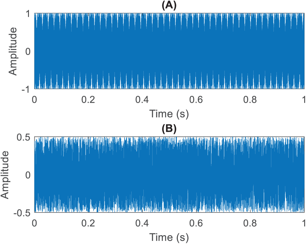
Figure 8: Original simulated automotive radar signals: (A) raw radar echo signal, and (B) external noise interference signal

As shown in Fig. 9, the original echo is decomposed into multiple IMFs via VMD, with each IMF represented by a distinct color. Since the original echo exhibits a linear frequency-modulated (chirp) characteristic, each mode reveals a relatively systematic increasing and decreasing frequency pattern, and the amplitude demonstrates a corresponding stratified structure. The blue trace (Mode 1) carries the slowest, highest-energy beat component; the orange and yellow traces (Modes 2 and 3) capture the first two harmonics, while the purple and green traces (Modes 4 and 5) contain higher-order, lower-amplitude details.

Figure 9: VMD-based analysis of the (A) signal from Fig. 8, showing the original simulated automotive radar echo

In Fig. 10, the horizontal axis represents time (s), the vertical axis denotes frequency (Hz), and the color intensity indicates energy magnitude. Several stable and continuous frequency bands can be observed, consistent with the linear sweeping behavior of the original chirp signal. The brighter regions signify higher energy, indicating that the echo signal amplitude is stronger at those instantaneous frequencies. Specifically, three dominant ridges appear at about 1, 2, and 4 kHz, corresponding to the fundamental beat tone and its first two harmonics for a 50 m target. This clear, band-limited pattern provides a reliable basis for extracting range and velocity in later processing stages.

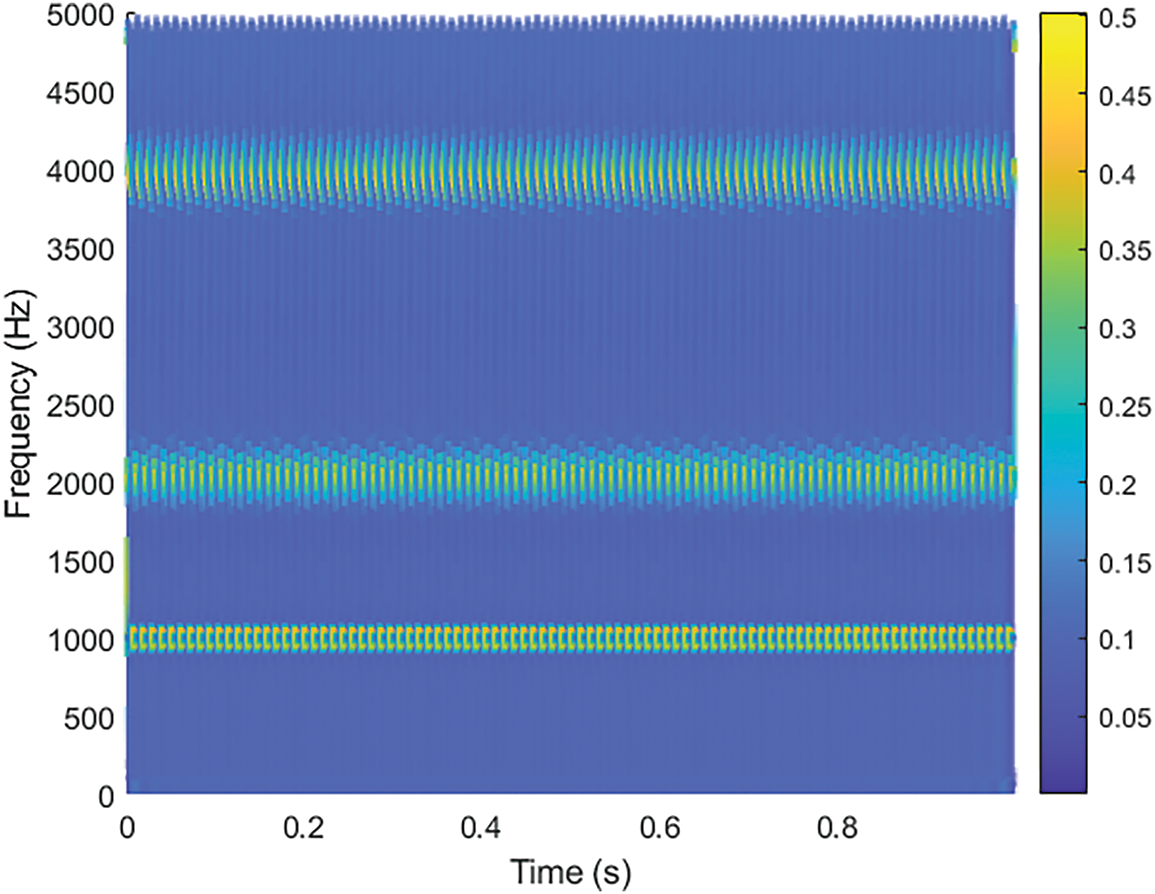
Figure 10: HHT-based analysis (after VMD) of the (A) signal from Fig. 9, showing the original simulated automotive radar echo

Fig. 11 illustrates the workflow after separation and correction of the mixed signals using the enhanced ICA approach combined with VMD analysis, where the “clean echo” is first decomposed via VMD and then multiplied by the original transmit signal to generate the difference frequency. A FFT is then applied to this difference signal, and the beat frequency peak f^b is located to estimate the target range. The x-axis represents frequency in hertz (0–20 Hz), whereas the y-axis displays the FFT magnitude in arbitrary linear units. The FFT is computed on a 1-s record (10,000 samples) after a Hann window and 10× zero-padding, giving a frequency resolution of 0.1 Hz; the resulting noise floor appears as a shallow ripple below 100 units. The principal peak is observed near 3.3 Hz, corresponding closely to the theoretical value of 3.333 Hz. Computations ultimately yield a theoretical distance of 50.00 m and an estimated distance of 49.50 m, indicating an error of merely 0.5 m. This result demonstrates that the multi-stage signal processing framework maintains accuracy under high noise conditions. The enhanced ICA approach not only effectively suppresses noise but also employs RLS to correct channel gain and phase mismatches, thereby preserving echo quality. Consequently, the beat-frequency identification aligns closely with theoretical expectations, and the derived distance deviates only slightly. Such performance underscores the method’s potential for robust target detection and range measurement in practical automotive radar scenarios.

Figure 11: Range estimation results (FFT) for the echo signal in Fig. 5A after enhanced ICA processing

The enhanced ICA algorithm proposed in this study successfully partitions the mixed signals into “clean echo” and “interference noise,” substantially enhancing the subsequent accuracy of radar-based distance or velocity estimations. By contrast, relying solely on the original echo or noise signal would offer limited utility in real-world conditions. These findings confirm the effectiveness of multi-channel signal processing in mitigating external environmental interference, thus providing strong evidence for the design and deployment of multi-channel radars in intelligent vehicles and ADAS.

The paragraph defines four objective metrics—output SNR, SNR gain (difference between input and output SNR), MSE, and Range-RMSE—and applies them to a 50-trial Monte-Carlo experiment with an input SNR of 12.7 dB. Averaged results show an output SNR of 20.3 dB, corresponding to an SNR gain of 7.6 dB. The mean-squared error is 0.25 m2, while the Range-RMSE is 0.50 m, yielding a residual range error of 1% relative to the 50 m ground-truth distance. These figures demonstrate that the proposed ICA-RLS-VMD/HHT pipeline substantially enhances noise suppression and preserves high range-estimation accuracy under challenging noise conditions, thereby providing a quantitative benchmark for subsequent comparative studies. Future work will employ the same metric set to conduct a systematic comparison against three representative baselines—standard ICA, wavelet-based filtering, or deep learning-based denoising—in order to quantify more precisely the strengths and limitations of the proposed framework in both noise reduction and range-estimation accuracy.

A VMD-parameter sensitivity study has been added to the paragraph. Forty-five combinations—modes K = 3–7, bandwidth factors α = 40 k/60 k/80 k rad s−1, and coupling weights γ = 40/70/100—were tested over 20 Monte-Carlo runs each. Results show that optimum performance occurs at K of approximately 5 ± 1, α in the 50–70 k rad s−1 band, and γ of approximately 70: fewer modes cause mode-mixing, more modes dilute energy; α < 40 k under-fits, α > 80 k slows execution (by about 25 percent) without benefit; γ > 100 begins to attenuate the echo. Practitioners are advised to start with K = 5, sweep α in 50–70 k rad s−1, and set γ around 70 (adding 10–15 when input SNR is below 10 dB).

Evaluate the algorithm’s computational demands in terms of processing time and memory usage, and discuss its feasibility for real-time automotive applications (e.g., FPGA, DSP, or embedded SoC platforms). On an Intel i7-9700 (single thread, MATLAB), the complete pipeline—ICA followed by RLS, five-mode VMD with thirty iterations, HHT, and a zero-padded radix-4 FFT—processes a one-second frame in 6.4 ms and peaks at about 6 MB of working memory. Runtime is dominated by the FFT-based VMD update and the final FFT, both of which are highly parallelisable. Future work will evaluate migrating the complete algorithm to embedded targets—a Kintex-7 FPGA and a Cortex-A53 SoC—and, through hardware-in-the-loop testing, verify that key resource metrics (under 40% LUT, under 20% BRAM, sub-1 ms pipeline latency, and 25 ms end-to-end runtime) are satisfied, thereby establishing its feasibility for real-time automotive-radar applications.

5  Conclusion

This study presents an integrated multi-stage signal processing framework for enhancing automotive FMCW radar performance. Initially, we model the FMCW echo and introduce multi-channel mixing to reflect real scenarios with amplitude mismatches and random noise. Then, an enhanced ICA separates the two radar echoes. Because amplitude and phase mismatches persist, we apply an RLS filter for calibration, refining the echo to align with the original measurement and reducing residual interference. After ICA-RLS, we employ VMD to decompose the calibrated echo into multiple IMFs, thereby isolating potential noise-dominated components. Additionally, the HHT exposes time-frequency structures, clarifying instantaneous frequencies that correspond to target parameters such as distance and velocity. Finally, we reconstruct a clean signal from selected IMFs and detect the beat frequency via HHT. Empirical results demonstrate that this dual-radar pipeline—ICA separation, RLS calibration, and VMD/HHT-based refinement—effectively mitigates interference while preserving the echo signature. The estimated distance closely matches theoretical calculations, indicating strong robustness and accuracy. This approach provides a reliable basis for automotive radar sensing in harsh conditions, where stable and accurate measurements are crucial, and supports ADAS and practicality. Empirical testing on 50 Monte-Carlo trials (input SNR = 12.7 dB) shows that the full processing pipeline lifts the output SNR to 20.3 dB (a 7.6 dB gain), achieves an MSE of 0.25 m2, and yields a Range-RMSE of 0.50 m, corresponding to a residual range error of roughly 1% relative to the 50 m ground-truth distance. Future work will focus on validating the proposed ICA and VMD/HHT pipeline with real-world measurements collected from a commercial 77 GHz mmWave FMCW radar module. This forthcoming study will examine performance under multipath, mutual-interference, and weather-induced clutter to confirm the framework’s robustness in practical ADAS scenarios.

Acknowledgement: Not applicable.

Funding Statement: The author would like to thank the National Science and Technology Council, Taiwan, for financially supporting this research (grant No. NSTC 113-2221-E-018-011) and the Ministry of Education’s Teaching Practice Research Program, Taiwan (PSK1134099).

Availability of Data and Materials: Not applicable.

Ethics Approval: Not applicable.

Conflicts of Interest: The author declares no conflicts of interest to report regarding the present study.

References

1. Kronauge M, Rohling H. New chirp sequence radar waveform. IEEE Trans Aerosp Electron Syst. 2014;50(4):2870–7. doi:10.1109/taes.2014.120813. [Google Scholar] [CrossRef]

2. Venon A, Dupuis Y, Vasseur P, Merriaux P. Millimeter wave FMCW RADARs for perception, recognition and localization in automotive applications: a survey. IEEE Trans Intell Veh. 2022;7(3):533–55. doi:10.1109/TIV.2022.3167733. [Google Scholar] [CrossRef]

3. Rameez M, Pettersson MI, Dahl M. Interference compression and mitigation for automotive FMCW radar systems. IEEE Sens J. 2022;22(20):19739–49. doi:10.36227/techrxiv.19753057.v1. [Google Scholar] [CrossRef]

4. Haider A, Eryildirim A, Pigniczki M, Haas L, Schlager B, Zeh T, et al. Modeling and simulation of automotive FMCW RADAR sensor for environmental perception. IEEE Open J Intell Transp Syst. 2025;6(2):433–55. doi:10.1109/ojits.2025.3554452. [Google Scholar] [CrossRef]

5. Wang J, Li R, Zhang X, He Y. Interference mitigation for automotive FMCW radar based on contrastive learning with dilated convolution. IEEE Trans Intell Transp Syst. 2024;25(1):545–58. doi:10.1109/TITS.2023.3306576. [Google Scholar] [CrossRef]

6. Wang Y, Huang Y, Wen C, Zhou X, Liu J, Hong W. Mutual interference mitigation for automotive FMCW radar with time and frequency domain decomposition. IEEE Trans Microw Theory Tech. 2023;71(11):5028–44. doi:10.1109/TMTT.2023.3275816. [Google Scholar] [CrossRef]

7. Sun R, Suzuki K, Owada Y, Takeda S, Umehira M, Wang X, et al. A millimeter-wave automotive radar with high angular resolution for identification of closely spaced on-road obstacles. Sci Rep. 2023;13(1):3233. doi:10.1038/s41598-023-30406-4. [Google Scholar] [PubMed] [CrossRef]

8. Alland S, Stark W, Ali M, Hegde M. Interference in automotive radar systems: characteristics, mitigation techniques, and current and future research. IEEE Signal Process Mag. 2019;36(5):45–59. doi:10.1109/MSP.2019.2908214. [Google Scholar] [CrossRef]

9. Hakobyan G, Yang B. High-performance automotive radar: a review of signal processing algorithms and modulation schemes. IEEE Signal Process Mag. 2019;36(5):32–44. doi:10.1109/MSP.2019.2911722. [Google Scholar] [CrossRef]

10. Nikandish R, Yousefi A, Mohammadi E. Spurs in millimeter-wave FMCW radar system-on-chip. IEEE Trans Radar Syst. 2023;1:21–33. doi:10.1109/trs.2023.3265845. [Google Scholar] [CrossRef]

11. Yan B, Roberts IP. Advancements in millimeter-wave radar technologies for automotive systems: a signal processing perspective. Electronics. 2025;14(7):1436. doi:10.3390/electronics14071436. [Google Scholar] [CrossRef]

12. Doris K, Filippi A, Jansen F. Reframing fast-chirp FMCW transceivers for future automotive radar: the pathway to higher resolution. IEEE Solid State Circuits Mag. 2022;14(2):44–55. doi:10.1109/MSSC.2022.3167344. [Google Scholar] [CrossRef]

13. Arai T, Usugi T, Murakami T, Kishimoto S, Utagawa Y, Kohtani M, et al. A 77-GHz 8RX3TX transceiver for 250-m long-range automotive radar in 40-nm CMOS technology. IEEE J Solid State Circuits. 2021;56(5):1332–44. doi:10.1109/JSSC.2021.3050306. [Google Scholar] [CrossRef]

14. Caffa M, Bottigliero S, Ramonda F, Gioanola L, Maggiora R. Integrated design and prototyping of a 77 GHz automotive medium range radar into car rear lamp. IEEE Trans Veh Technol. 2023;73(3):3041–50. doi:10.1109/TVT.2023.3324986. [Google Scholar] [CrossRef]

15. Eder Y, Eldar YC. Sparsity-based multi-person non-contact vital signs monitoring via FMCW radar. IEEE J Biomed Health Inform. 2023;27(6):2806–17. doi:10.1109/JBHI.2023.3255740. [Google Scholar] [PubMed] [CrossRef]

16. Gupta S, Rai PK, Kumar A, Yalavarthy PK, Cenkeramaddi LR. Target classification by mmWave FMCW radars using machine learning on range-angle images. IEEE Sens J. 2021;21(18):19993–20001. doi:10.1109/JSEN.2021.3092583. [Google Scholar] [CrossRef]

17. Shamsfakhr F, Macii D, Palopoli L, Corrà M, Ferrari A, Fontanelli D. A multi-target detection and position tracking algorithm based on mmWave-FMCW radar data. Measurement. 2024;234(11):114797. doi:10.1016/j.measurement.2024.114797. [Google Scholar] [CrossRef]

18. Hyvärinen A, Oja E. Independent component analysis: algorithms and applications. Neural Netw. 2000;13(4–5):411–30. doi:10.1016/s0893-6080(00)00026-5. [Google Scholar] [PubMed] [CrossRef]

19. Tharwat A. Independent component analysis: an introduction. Appl Comput Inform. 2021;17(2):222–49. doi:10.1016/j.aci.2018.08.006. [Google Scholar] [CrossRef]

20. Mehta PK, Kumaraswamy A, Saraswat VK, Chinnadurai V, Kumar BP. Prediction of material properties of propellant waste modified bricks through microstructures by Topographic independent component analysis coupled 3D Convolution neural networks. Ceram Int. 2022;48(19):28918–26. doi:10.1016/j.ceramint.2022.04.064. [Google Scholar] [CrossRef]

21. Engel Y, Mannor S, Meir R. The kernel recursive least-squares algorithm. IEEE Trans Signal Process. 2004;52(8):2275–85. doi:10.1109/tsp.2004.830985. [Google Scholar] [CrossRef]

22. Benesty J, Paleologu C, Gänsler T, Ciochină S. Recursive least-squares algorithms. In: A perspective on stereophonic acoustic echo cancellation. Berlin/Heidelberg, Germany: Springer; 2011. [Google Scholar]

23. Paleologu C, Benesty J, Ciochina S. Data-reuse recursive least-squares algorithms. IEEE Signal Process Lett. 2022;29:752–6. doi:10.1109/lsp.2022.3153207. [Google Scholar] [CrossRef]

24. Huang NE, Shen Z, Long SR, Wu MC, Shih HH, Zheng Q, et al. The empirical mode decomposition and the Hilbert spectrum for nonlinear and non-stationary time series analysis. Proc R Soc Lond A. 1998;454(1971):903–95. doi:10.1098/rspa.1998.0193. [Google Scholar] [CrossRef]

25. Huang NE, Shen Z, Long SR. A new view of nonlinear water waves: the Hilbert Spectrum. Annu Rev Fluid Mech. 1999;31(1):417–57. doi:10.1146/annurev.fluid.31.1.417. [Google Scholar] [CrossRef]

26. Wu Z, Huang NE. Ensemble empirical mode decomposition: a noise-assisted data analysis method. Adv Adapt Data Anal. 2009;1(1):1–41. doi:10.1142/s1793536909000047. [Google Scholar] [CrossRef]

27. Randall RB, Antoni J. Why EMD and similar decompositions are of little benefit for bearing diagnostics. Mech Syst Signal Process. 2023;192(5):110207. doi:10.1016/j.ymssp.2023.110207. [Google Scholar] [CrossRef]

28. Dragomiretskiy K, Zosso D. Variational mode decomposition. IEEE Trans Signal Process. 2014;62(3):531–44. doi:10.1109/tsp.2013.2288675. [Google Scholar] [CrossRef]

29. Rehman NU, Aftab H. Multivariate variational mode decomposition. IEEE Trans Signal Process. 2019;67(23):6039–52. doi:10.1109/tsp.2019.2951223. [Google Scholar] [CrossRef]

30. Nazari M, Sakhaei SM. Successive variational mode decomposition. Signal Process. 2020;174(1971):107610. doi:10.1016/j.sigpro.2020.107610. [Google Scholar] [CrossRef]

31. Moreno SR, Seman LO, Stefenon SF, dos Santos Coelho L, Mariani VC. Enhancing wind speed forecasting through synergy of machine learning, singular spectral analysis, and variational mode decomposition. Energy. 2024;292:130493. doi:10.1016/j.energy.2024.130493. [Google Scholar] [CrossRef]

32. Gu J, Peng Y, Lu H, Chang X, Chen G. A novel fault diagnosis method of rotating machinery via VMD, CWT and improved CNN. Measurement. 2022;200(5):111635. doi:10.1016/j.measurement.2022.111635. [Google Scholar] [CrossRef]

33. Hadiyoso S, Dewi EM, Wijayanto I. VMD and EEMD methods in respiration wave extraction based on PPG waves. J Phys Conf Ser. 2020;1577(1):012040. doi:10.1088/1742-6596/1577/1/012040. [Google Scholar] [CrossRef]

34. Chen T, Gao S, Zheng S, Yu S, Xuan Q, Lou C, et al. EMD and VMD empowered deep learning for radio modulation recognition. IEEE Trans Cogn Commun Netw. 2023;9(1):43–57. doi:10.1109/tccn.2022.3218694. [Google Scholar] [CrossRef]

35. Seyrek P, Şener B, Özbayoğlu AM, Ünver HÖ. An evaluation study of EMD, EEMD, and VMD for chatter detection in milling. Procedia Comput Sci. 2022;200(1):160–74. doi:10.1016/j.procs.2022.01.215. [Google Scholar] [CrossRef]

36. Yun X, Jian R. Features method for selecting VMD parameters based on spectrum without modal overlap. J Phys Conf Ser. 2020;1605(1):012002. doi:10.1088/1742-6596/1605/1/012002. [Google Scholar] [CrossRef]

37. Zhao S, Wu Y, Jiang X, Peng D, Yu J. Weak signal detection in chaotic noise background—based on VMD-EEMD and self-attention mechanisms. J Phys Conf Ser. 2024;2851(1):012015. doi:10.1088/1742-6596/2851/1/012015. [Google Scholar] [CrossRef]

38. Lin SL, Tung PC, Huang NE. Data analysis using a combination of independent component analysis and empirical mode decomposition. Phys Rev E Stat Nonlin Soft Matter Phys. 2009;79(6):066705. doi:10.1103/physreve.79.066705. [Google Scholar] [PubMed] [CrossRef]

39. Lin SL, Tung PC, Huang NE. Application of ICA-EEMD to secure communications in chaotic systems. Int J Mod Phys C. 2012;23(4):1250028. doi:10.1142/s0129183112500283. [Google Scholar] [CrossRef]

40. Lin SL. Application combining VMD and ResNet101 in intelligent diagnosis of motor faults. Sensors. 2021;21(18):6065. doi:10.3390/s21186065. [Google Scholar] [PubMed] [CrossRef]

41. Lin SL. Application of empirical mode decomposition to improve deep learning for US GDP data forecasting. Heliyon. 2022;8(1):e08748. doi:10.1016/j.heliyon.2022.e08748. [Google Scholar] [PubMed] [CrossRef]

42. Lin SL. The application of machine learning ICA-VMD in an intelligent diagnosis system in a low SNR environment. Sensors. 2021;21(24):8344. doi:10.3390/s21248344. [Google Scholar] [PubMed] [CrossRef]

43. Von Kügelgen J, Sharma Y, Gresele L, Brendel W, Schölkopf B, Besserve M, et al. Self-supervised learning with data augmentations provably isolates content from style. Adv Neural Inf Process Syst. 2021;34:16451–67. [Google Scholar]

44. Geirhos R, Jacobsen JH, Michaelis C, Zemel R, Brendel W, Bethge M, et al. Shortcut learning in deep neural networks. Nat Mach Intell. 2020;2(11):665–73. doi:10.1038/s42256-020-00257-z. [Google Scholar] [CrossRef]

45. Farahani FV, Karwowski W, Lighthall NR. Application of graph theory for identifying connectivity patterns in human brain networks: a systematic review. Front Neurosci. 2019;13:585. doi:10.3389/fnins.2019.00585. [Google Scholar] [PubMed] [CrossRef]

46. Alibakhshi-Kenari M, Movahhedi M, Naderian H. A new miniature ultra wide band planar microstrip antenna based on the metamaterial transmission line. In: 2012 IEEE Asia-Pacific Conference on Applied Electromagnetics (APACE); 2012 Dec 11–13; Melaka, Malaysia. p. 293–7. doi:10.1109/APACE.2012.6457679. [Google Scholar] [CrossRef]

47. Alibakhshi-Kenari M, Naser-Moghadasi M, Virdee BS, Andújar A, Anguera J. Compact antenna based on a composite right/left-handed transmission line. Microw Opt Technol Lett. 2015;57(8):1785–8. doi:10.1002/mop.29191. [Google Scholar] [CrossRef]

48. Skolnik MI. Radar handbook. 3rd ed. New York, NY, USA: McGraw-Hill; 2008. [Google Scholar]

49. Richards MA. Fundamentals of radar signal processing. 3rd ed. New York, NY, USA: McGraw-Hill; 2022. [Google Scholar]

50. Hyvarinen A. Fast and robust fixed-point algorithms for independent component analysis. IEEE Trans Neural Netw. 1999;10(3):626–34. doi:10.1109/72.761722. [Google Scholar] [PubMed] [CrossRef]

51. Hyvärinen A, Oja E. A fast fixed-point algorithm for independent component analysis. Neural Comput. 1997;9(7):1483–92. doi:10.1162/neco.1997.9.7.1483. [Google Scholar] [CrossRef]

52. Cardoso JF. High-order contrasts for independent component analysis. Neural Comput. 1999;11(1):157–92. doi:10.1162/089976699300016863. [Google Scholar] [PubMed] [CrossRef]