
 Submit a Paper
 Propose a Special lssue
 Open Access
ARTICLE
Fatigue Life Prediction of Composite Materials Based on BO-CNN-BiLSTM Model and Ultrasonic Guided Waves
1 College of Fiber Engineering and Equipment Technology, Jiangnan University, Wuxi, 214122, China
2 Harbin FRP Institute Co., Ltd., Harbin, 150000, China
* Corresponding Authors: Jun Li. Email: ; Dongyue Gao. Email:
(This article belongs to the Special Issue: Computing Technology in the Design and Manufacturing of Advanced Materials)
Computers, Materials & Continua 2025, 85(1), 597-612. https://doi.org/10.32604/cmc.2025.067907
Received 15 May 2025; Accepted 15 July 2025; Issue published 29 August 2025
 View Full Text
 Download PDF
Abstract
Throughout the composite structure’s lifespan, it is subject to a range of environmental factors, including loads, vibrations, and conditions involving heat and humidity. These factors have the potential to compromise the integrity of the structure. The estimation of the fatigue life of composite materials is imperative for ensuring the structural integrity of these materials. In this study, a methodology is proposed for predicting the fatigue life of composites that integrates ultrasonic guided waves and machine learning modeling. The method first screens the ultrasonic guided wave signal features that are significantly affected by fatigue damage. Subsequently, a covariance analysis is conducted to reduce the redundancy of the feature matrix. Furthermore, one-hot encoding is employed to incorporate boundary conditions as features, and the resulting data undergoes preprocessing to form a sample library. A composite fatigue life prediction model has been developed, employing the aforementioned sample library as the input source and utilizing remaining life as the output metric. The model synthesizes the strengths of convolutional neural networks (CNNs) and bidirectional long short-term memory networks (BiLSTMs) while leveraging Bayesian optimization (BO) to enhance the optimization of hyperparameters. The experimental results demonstrate that the proposed BO-CNN-BiLSTM model exhibits superior performance in terms of prediction accuracy and reliability in the damage regression task when compared to both the BiLSTM and CNN-BiLSTM models.Keywords
Composite materials, with their advantages of high specific strength/stiffness and designability, are increasingly used in aerospace applications. However, composites usually exhibit nonlinearities and generalized anisotropy, leading to more complex failure mechanisms and damage monitoring of these composite structures than conventional structures. When aerospace structures are subjected to alternating loads for a long period of time during their service life, fatigue damage in the form of fiber breakage, matrix cracking, debonding and delamination continue to accumulate in the structures and eventually lead to structural failure or a significant decline in performance [1,2]. Consequently, there is an imperative need to develop effective fatigue life prediction models to ensure the safety and reliability of these structures. A significant number of researchers are concentrating on the study of fatigue life prediction in composite materials. Lai et al. investigated the fatigue damage characteristics of carbon fiber-reinforced composites and their life prediction methods. The validity of the proposed prediction method was verified by finite element analysis, which demonstrated its reliability and provided support for enhancing the structural safety of composites [3]. Dong et al. proposed a fatigue damage evolution equation based on acoustic emission signals. This equation was developed for the purpose of accurately tracking the damage progression and predicting the fatigue life of composite laminates. The experimental results demonstrate the efficacy of the method in capturing the characteristics of initial damage, steady-state damage, and accelerated damage during fatigue. This result provides an important theoretical basis and practical application potential for structural health monitoring and fatigue life prediction of composite materials [4]. Structural Health Monitoring (SHM) technologies have been demonstrated to play a vital role in mitigating the risk of failure under harsh operational loads and environmental conditions. These technologies have also been shown to reduce the costs associated with prolonged downtime during regular inspection and maintenance [5–9]. Piezoelectric signal measurement has been widely used as an effective sensing technique in health monitoring of composite structures, while artificial intelligence techniques can effectively process the data to improve the accuracy and efficiency of damage detection [10,11].
Piezoelectric materials can produce electrode polarization phenomenon under external stress or deformation under electric field stimulation [12]. Therefore, sensors based on the piezoelectric effect can be used as multifunctional sensors to realize SHM by various technological means, such as electromechanical impedance [13,14], ultrasonic guided wave [15], acoustic emission [16], and stress monitoring [17], etc. Among them, ultrasonic guided waves have the advantages of being able to propagate long distances in structures and being sensitive to damages such as cracks, debonding and delamination [18,19], which can realize the quantitative identification of damages such as microcracks and debonding inside large plate and shell structures. Therefore, the use of ultrasonic guided waves for damage monitoring is widely recognized in the field of aerospace structural overhaul and reliability research. In the study of structural health monitoring based on ultrasonic guided waves, machine learning algorithms offer superior data processing and pattern recognition capabilities. They can accurately capture subtle changes in structural damage, which are reflected in ultrasonic guided wave signals. These algorithms also demonstrate high accuracy and significant potential in predicting fatigue life [20–22]. The efficacy of machine learning models is contingent upon the quality of the input data, particularly the selection and extraction of features. It is evident that a solitary feature is incapable of adequately reflecting the intricate damage mechanism of composite materials [23]. Consequently, enhancing the accuracy of predictions necessitates the extraction of numerous features that comprehensively mirror the damage state. Subsequent to the extraction of features, the selection of an appropriate machine model is imperative for optimizing prediction performance. Among them, recurrent neural network (RNN) is able to share the parameters of different time steps in a time series by establishing recurrent connections between hidden layer neurons, effectively retaining historical information, and is suitable for processing time series data, but it is prone to gradient disappearance or gradient explosion when processing time series data [24]. To address this, the bidirectional long and short-term memory network (BiLSTM) builds upon the RNN by introducing “memory units” and “gating mechanisms”, such as forgetting, input, and output gates. These mechanisms control the flow of information, allowing BiLSTM to effectively handle long-term dependencies in sequences [25]. BiLSTM overcomes the limitations of traditional RNN, and as a result, it is widely used for predicting composite fatigue damage in time series. Although BiLSTM can effectively process time series data, it has limitations in capturing local patterns and deep features in the data, which leads to a model that may not be adequate in feature extraction. Convolutional neural network (CNN) excel in local feature extraction and can effectively recognize spatial patterns in data. In order to fully utilize the advantages of both, this paper combines CNN and BiLSTM with the aim of providing a more comprehensive assessment of the safety of composite fatigue damage. However, a major challenge is faced when combining CNN and BiLSTM models: due to the complex structure of the model and the large hyperparameter space, the process of finding the optimal hyperparameters becomes more difficult. In order to solve this problem, this study applies Bayesian Optimization (BO) for hyperparameter optimization [26,27]. As an efficient optimization method, Bayesian optimization can efficiently approximate optimal hyperparameters with limited trials, which is especially suitable for solving high-dimensional and computationally expensive optimization problems. Therefore, in this paper, the Bayesian optimization algorithm is chosen to optimize the hyperparameters of CNN and BiLSTM models, so as to improve the prediction accuracy and computational efficiency of the models.
The main contributions of this paper are as follows:
1. Construction of a CNN-BiLSTM model for composite material fatigue life prediction: The model combines a CNN for feature extraction and a BiLSTM for capturing long-term dependencies. It is engineered for the specific purpose of assessing the fatigue life of composite materials.
2. Introducing the Bayesian Optimization (BO) algorithm for hyperparameter optimization: The BO algorithm is used to optimize the model’s hyperparameters, which significantly improves the model’s accuracy and reliability in fatigue life prediction.
The subsequent sections of the paper are structured as follows: the section on composite fatigue loading damage diagnostic tests describes the dataset and the steps involved in data preprocessing. The section on composite fatigue life prediction method based on BO-CNN-BiLSTM model describes the structure and training of the proposed neural network model. The section entitled “Results and Discussion” is where the findings from the training of the proposed neural network model are described, as well as the comparison of that model with other models. In conclusion, the final section of the text offers a summary of the work’s main points.
2 Composite Material Fatigue Loading Damage Diagnostic Test
The dataset used in this paper is the data from a fatigue aging test of CFRP composites conducted by the Stanford Structures and Composites Laboratory (SACL) in collaboration with the Center of Prediction of Excellence (PCoE) at NASA Ames Research Center [28]. In this test, a set of specimens were subjected to tensile-tensile fatigue tests under controlled cyclic loading at a frequency of 5.0 Hz and a stress ratio of R = 0.14, and the specimens are shown in Fig. 1.
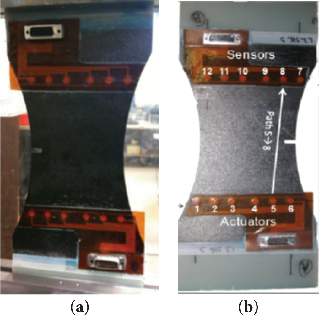
Figure 1: Schematic diagram of the test specimen [28]. (a) Preparation of the specimen for testing (b) Schematic diagram of the signal path, exciter (1–6) and receiver (7–12)
The specimens were fabricated using Torayca T700G unidirectional carbon prepreg with dimensions of 15.24 cm × 25.4 cm, and a notch of 5.08 mm × 19.3 mm was created in the specimen to induce stress concentration. The tests were conducted for three composite specimens with different layup configurations, all of which were carried out on an MTS testing machine. The sending and receiving of ultrasonic guided wave signals was realized by 12 PZT transducers, which included 6 exciters and 6 receivers, forming a total of 36 signal paths. Seven excitation frequencies were set up in the range of 150–450 kHz in steps of 50 kHz, and the average input voltage of the excitation signals was 50 V. The fatigue cycling test was stopped at a specific number of fatigue cycles, and the PZT sensor data were collected for all the paths and frequencies while the specimens were imaged by X-rays. The monitoring data consisted of Lamb wave signals collected from the PZT sensor network and fatigue damage extension observed by X-ray imaging.
The present paper selects four specimens with a layer configuration of [02/904]s, namely L1S11, L1S12, L1S18, and L1S19. Taking specimen L1S19 as an example, Fig. 2 shows the guided wave signals collected with 300 kHz as the excitation frequency for the 6#→7# signal path under different fatigue cycle times. As shown in the figure, the specimen gradually sustains damage as the number of fatigue cycles increases, leading to signal energy attenuation during propagation. This attenuation reflects the accumulation of internal damage within the material and is associated with microstructural changes. Additionally, the frequency characteristics and amplitude of the signal change across different fatigue stages, particularly the shift in the peak position of the signal. Concurrently, the signal exhibits nonlinear variation. Nonlinear changes mean that signal attenuation is not a simple, uniform decrease but accelerates or undergoes sudden changes after a certain number of fatigue cycles. This phenomenon is typically associated with crack propagation, localized failure, or sudden changes in the material’s microstructure. As the number of loading cycles increases during the fatigue process, the extent of damage to the specimen worsens, leading to sudden changes in signal amplitude and frequency characteristics. These changes reflect the nonlinear process of damage accumulation in the material. Overall, the signal changes exhibit a certain degree of regularity in relation to the number of fatigue cycles, providing important reference criteria for predicting and evaluating fatigue damage.
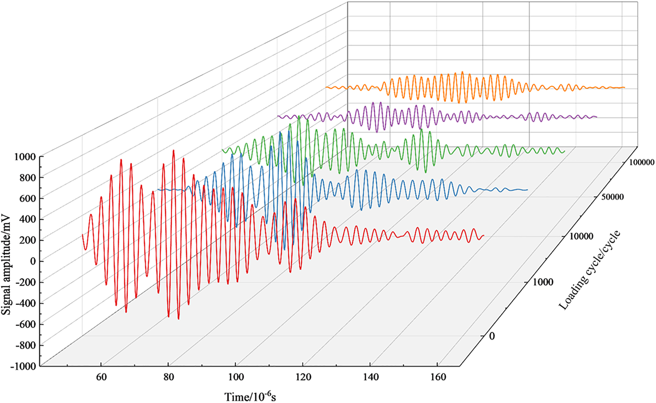
Figure 2: Lamb wave signals with different number of fatigue cycles in path 6#→7# at 300 kHz
2.2 Characterization of Specimen Fatigue Damage
As L1S19 in point, the experimental results of the specimen under different cycle tensile times are shown in Fig. 3, (a) is the X-ray image when the cycle tensile number is 20,000, (b) is the change curve of the damage size with the cycle number, with the increase of the cycle number, the damage area gradually increases, and it can be seen that the damage size has experienced a typical three-phase evolution process of budding-expansion-accelerated failure, which is closely related to the fatigue cumulative effect of the specimen. According to the on-site description, specimen L1S19 emitted a cracking sound at 125,000 cycles, and the load no longer increased during the loading process. Ultrasonic guided wave data could no longer be collected. After unloading, X-ray results showed extensive delamination inside the specimen. Upon inspection, most of the sensors were found to be damaged. Therefore, it was determined that the specimen failed completely when the fatigue load reached 125,000 cycles.
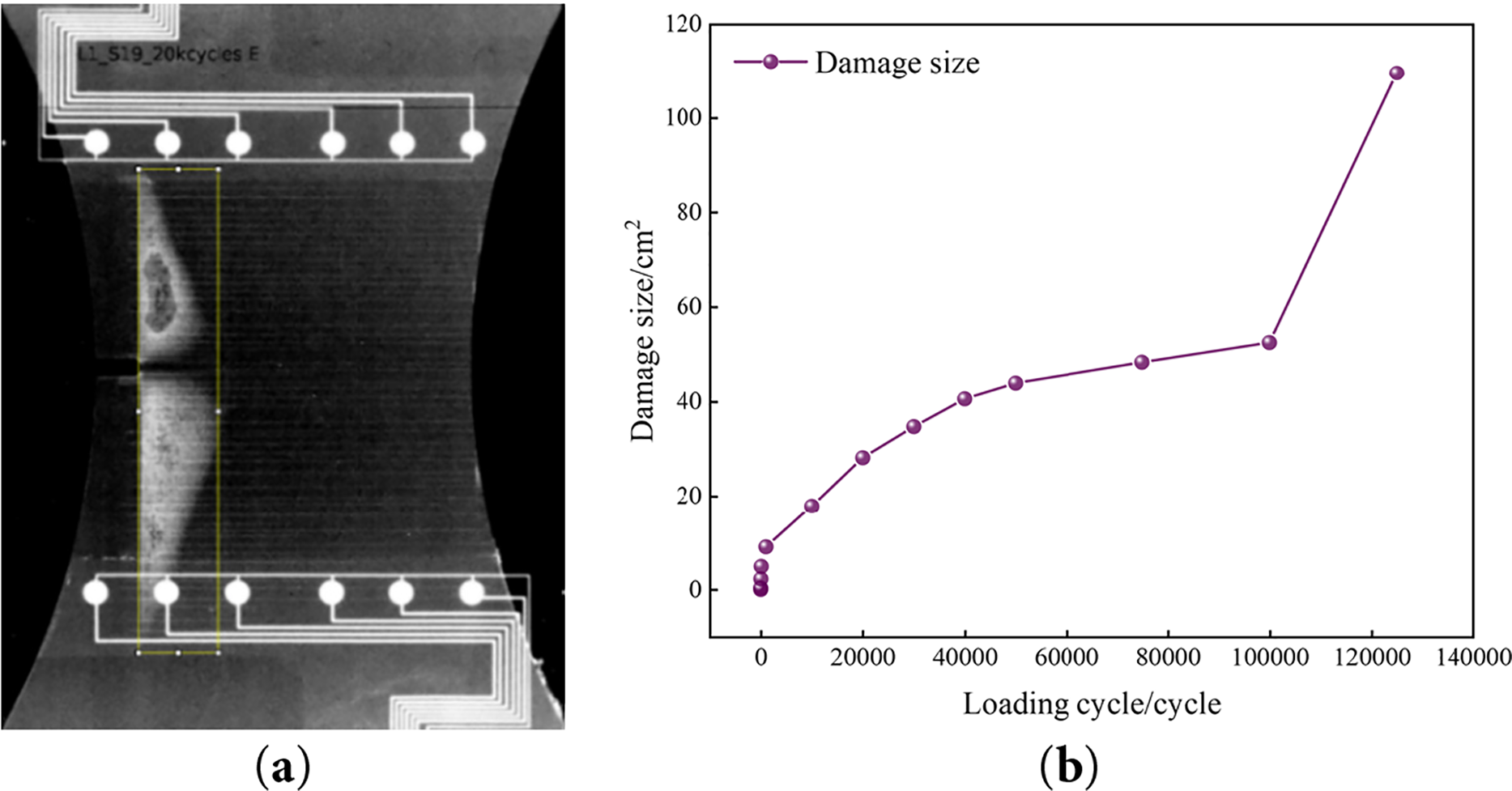
Figure 3: Damage dimensions of specimens at different numbers of stretching. (a) X-ray image at 20,000 cycles of stretching (b) Variation curve of damage dimensions with the number of cycles
In the process of model building, extracting damage-related features to improve the model capability is an important issue. And too many features may increase training time and introduce irrelevant information, affecting prediction accuracy. Therefore, in the process of damage prediction model building, feature selection is needed, and the features should be representative enough to ensure the efficiency of the model operation.
Fatigue damage alters material properties and morphological dimensions. These changes affect guided wave propagation constitutive equations and boundary conditions, thereby modifying ultrasonic guided wave signal characteristics (e.g., amplitude, arrival time, frequency distribution). This change is mainly reflected in the amplitude of the guided wave signal, arrival time, frequency distribution and signal complexity. In previous studies, the seven signal characteristics listed in Table 1 are typically used to characterize the damage parameters.
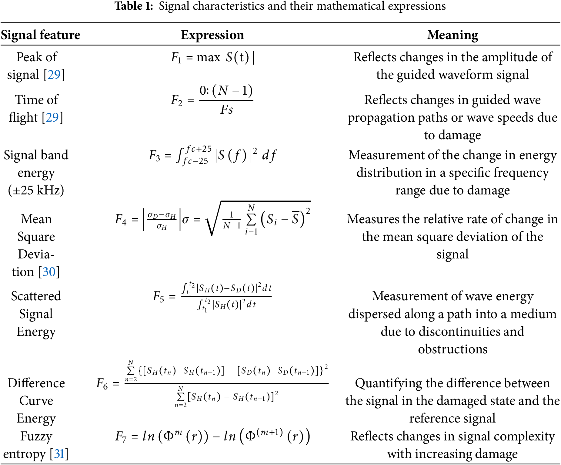
The above features can comprehensively characterize the effect of damage on the ultrasonic guided wave signal from multiple dimensions, providing high-quality input data for the subsequent BO-CNN-BiLSTM model.
Meanwhile, in order to improve the model’s generalization ability and prediction accuracy, and to better identify and process highly correlated features in the dataset, this study uses the Pearson correlation coefficient to measure the correlation between features, which is calculated as shown in the following equation.
In Eqs. (1) and (2):
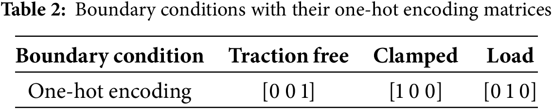
The test was conducted at seven different driving frequencies, and 36 signal transmission paths were designed and constructed using a sensor network in order to fully capture the guided wave response of the structure under different conditions. The data collected through these pathways are as follows: L1S11 contains 145 groups, L1S12 contains 109 groups, L1S18 contains 179 groups, and L1S19 contains 82 groups. Given that the guided wave signals obtained from each signal path may carry critical information at different frequencies, the contributions from all signal sources are combined in the data processing. Firstly, the signals were subjected to Fourier transform processing to extract more signal features from the frequency domain. The final set of features comprised seven distinct components: peak value, TOF value, signal ±25 kHz band energy, mean square deviation, scattered signal energy, differential curve energy, and fuzzy entropy. However, there may be a significant linear relationship between these seven features, which affects the prediction performance of the model, so covariance analysis needs to be done on the extracted features to eliminate redundant features, improve the efficiency of the model, and avoid the instability of prediction due to multiple covariance. The selected features are shown in Fig. 4b. A total of four features are finally identified to form the sample library, which are peak value, TOF value, scattered signal energy, and fuzzy entropy. Each working condition has different boundary conditions: Traction Free, Clamped, Load, which are incorporated into the feature data as inputs by using the one-hot encoding, and the one-hot encoding for different boundary conditions are shown in Table 2, which will provide rich data support for the subsequent fatigue damage analysis.
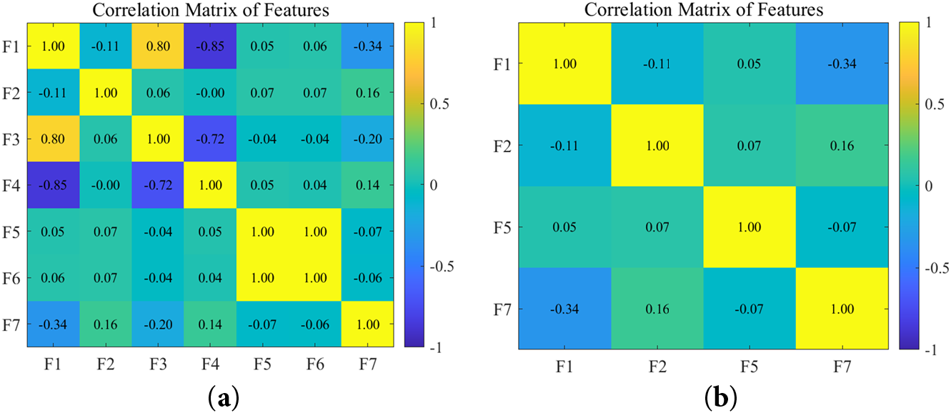
Figure 4: Heat map of covariance between features. (a) Relationship map before removing redundant features (b) Relationship map after removing redundant features
For each working condition, four kinds of features were extracted under seven different driving frequencies and 36 signal paths. The four features are fused with the one-hot encoding, and the final data structure for each working condition is 252 × 7. In order to make the prediction, the time step is set to 2, i.e., the data of the past two time steps are used to predict the value of the third time step, and a total of 507 groups of data are formed in the end, and the structure of the data for each group is 504 × 1 × 7. In this study, the specimen was deemed to have completely failed after undergoing the maximum number of cycles under load. Therefore, the maximum number of cycles were defined as the upper limit of the fatigue life of the structure. Based on this, the remaining life of other cycle counts can be calculated by normalizing the difference between the cycle count at failure and the corresponding cycle count. This indicator is used as the output label of the model to predict fatigue damage.
3 Composite Fatigue Life Prediction Method Based on BO-CNN-BiLSTM Model
In this paper, a method for ultrasonic guided wave monitoring of structural fatigue damage based on BO-CNN-BiLSTM model is proposed for the fatigue damage characteristics of composites. BiLSTM has demonstrated efficacy in addressing long-term dependencies in sequences. Its utilization in the prediction of fatigue damage to composites over time series is extensive. However, it is important to note that BiLSTM exhibits certain limitations in accurately capturing the local patterns and deep features in data. Therefore, it is necessary to combine BiLSTM with CNN and optimize the hyperparameters of the neural network using Bayesian optimization algorithm.
3.1 Composite Fatigue Life Prediction Model Based on BO-CNN-BiLSTM
In this study, an innovative method for the safe assessment of fatigue damage in composites is proposed, aiming to improve the accuracy and robustness of damage prediction. The method combines CNN, BiLSTM, and BO techniques, taking full advantage of each model in order to improve the overall performance of the assessment system.
The task of the CNN is to extract key local feature information from the feature matrix. The model’s input is the extracted feature matrix from the original guide wave signal. First, CNN is used to process the input data to mine key features that can effectively reflect the damage information. The data passes through the convolutional layer (CL) for local feature extraction, the convolutional kernel size is set to [128, 1], and the number of convolutional layers and neurons are automatically adjusted by the Bayesian optimization algorithm. Convolution layers capture local features and enhance the model’s learning ability by performing convolution operations on the input data. The formula for the convolution operation is shown in Eq. (3) below. In the equation,
After feature extraction, the BiLSTM network is used to deal with long-term dependencies in time series. The BiLSTM network is consists of “memory units” and “gating mechanisms” that can effectively capture the time series features in the data by dynamically regulating the flow of information. This improvs the model’s adaptability to dynamic changes. The bidirectional structure of BiLSTM can further enhance the model’s ability to learn from different time steps and make full use of historical information for prediction. The BiLSTM processing process can be described by Eqs. (5)–(7). In this equation,
However, when combining CNN with BiLSTM, the hyperparameter optimization of the model becomes a key issue. In the complex CNN-BiLSTM combination model, the choice of hyperparameters has a large impact on the robustness of the model [32]. For example, the size and number of layers of convolutional kernel, the number of units of BiLSTM hidden layer, the learning rate, the regularization coefficient, etc. need to be precisely adjusted. If the hyperparameters are not properly selected, it may lead to oscillation or slow convergence of the model in the training process, and even affect the final prediction accuracy of the model.
To address this problem, this study uses a Bayesian optimization algorithm to automatically optimize the hyperparameters in the neural network with a maximum of 30 iterations. Bayesian optimization improves the search efficiency and optimization accuracy by building a proxy model (e.g., Gaussian process) that selects the next set of hyperparameters intelligently, based on known hyperparameter configurations and model performance, in each iteration. In this study, Bayesian optimization is used to optimize several hyperparameters, such as the number of hidden layer units, minimum batch size, learning rate, and L2 regularization coefficient, to ensure optimal model performance during training. During the optimization process, BO uses Bayes’ theorem to update the posterior distribution of the objective function, as shown in Eq. (8). In this equation,
Compared to a single model, this integrated approach improves prediction accuracy and enhances the model’s robustness to better cope with complex damage prediction tasks. Fig. 5 illustrates the basic architecture of the proposed security assessment method.
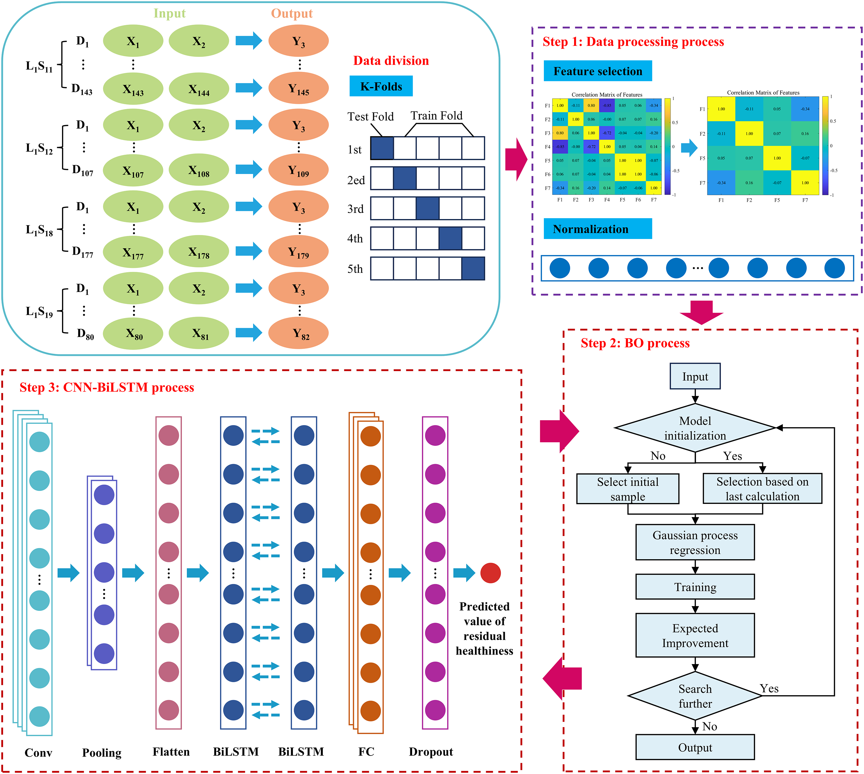
Figure 5: Overview of the proposed methodology
The BO-CNN-BiLSTM-based fatigue life prediction model has the following main steps:
Step 1: Construct the sample library. Damage-related features are extracted, and a covariance analysis is performed to eliminate redundant features. This process forms a signal feature matrix. The signal feature matrix is then combined with remaining life labels to form a sample library.
Step 2: Data processing. It is imperative to normalize the input data prior to training due to the varying scales across different features. This preprocessing step is crucial to mitigate the potential influence of particular features on the model, which might be amplified due to their substantial scale during training. This can lead to adverse effects on the model’s convergence and accuracy.
Step 3: Establish the hyperparameter search space. The initial step in the BO algorithm is the establishment of a suitable search space for the optimized hyperparameters. This search space encompasses various parameters, including the size of the convolution kernel, the number of layers, the number of BiLSTM hidden layer units, the learning rate, and the regularization coefficients, among others.
Step 4: Bayesian optimization. The Bayesian optimization algorithm utilizes Gaussian process regression to assess the objective function, thereby identifying the optimal configuration of hyperparameters. In this process, Expectation Improvement (EI) is employed as a collection function to guide the algorithm in selecting the subsequent set of hyperparameters.
Step 5: Model training and prediction. The normalized data is subsequently fed into the BO-CNN-BiLSTM model, which is processed by the convolutional, pooling, and bidirectional LSTM layers to finally obtain the predicted values. The objective of this step is to obtain the remaining life prediction results through the forward propagation process of the model.
Step 6: Objective function calculation and update. In the event that the prediction error of the model does not align with the predefined stopping criterion, the process is to revert to step 4 and proceed with hyperparameter update and model training. The process continues to iterate until the number of training sessions reaches a set value or the error meets the termination criteria.
Step 7: k-fold cross-validation. To ensure the stability and generalization ability of the model, k-fold cross-validation is used for evaluation. In this study, the k-value is set to 5, meaning that the sample data are randomly divided into 5 subsets. Each time, 4 of the subsets are used for training, and the remaining 1 subset is used for testing. The validation of each subset in succession ensures a comprehensive evaluation of the model’s performance, thereby circumventing the pitfalls of model overfitting.
Step 8: Model evaluation. The final step in the research process involves the evaluation of the model’s accuracy. This is achieved by employing various assessment metrics, including Root Mean Square Error (RMSE), Mean Absolute Error (MAE), and the Coefficient of Determination (R2). These metrics effectively measure the discrepancy between the model’s predictions and the actual values, thereby validating the model’s overall performance.
3.2 BO-CNN-BiLSTM Fatigue Life Prediction Model Training
Before model training, the dataset first needs to be divided, there are a total of 507 sets of data, and the training and test sets are divided according to the ratio of 8:2. The next step is data preprocessing, where the data are normalized using the following equation before predicting the fatigue damage dimensions of composites due to the different feature scales selected. Next, hyper-parameter selection is done through Bayesian optimization, where the combination of hyper-parameters selected and the training error of the model under this combination are saved, and finally the combination of hyper-parameters with the smallest error is obtained through comparison and used for the model training to get the prediction of the damage dimensions on the test set.
In Eq. (9):
The error of the BO-CNN model is evaluated using three metrics including Root Mean Square Error (RMSE), Mean Absolute Error (MAE), and Correlation Coefficient (R2), which are defined in the following equations:
In Eqs. (10)–(12):
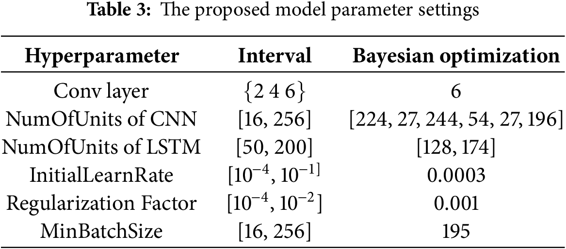
MAE is insensitive to outliers and pays more attention to the average deviation, the smaller the value is, the more accurate the prediction is; RMSE integrates the effect of error size and outliers, the smaller the value is, the more accurate the model prediction is; R2 is used to evaluate the model’s ability to explain the data, with a range of [0, 1], and the closer to 1, the better the model’s fitting effect is. Each of these metrics has its own focus and can reflect the prediction performance of the model at different levels. RMSE is more concerned with the effect of large errors, MAE is suitable for measuring the overall error level, and R2 emphasizes the model’s goodness-of-fit, and this use of multiple metrics can provide a more comprehensive assessment of the model performance. The prediction results of the model under k-fold cross-validation are displayed in Fig. 6. It has been observed that the model achieves optimal prediction outcomes when k = 3. Furthermore, Fig. 7 illustrates the iterative curve of the model at k = 3, demonstrating a significant overlap between the two curves. This observation indicates that the model has converged and identified the global optimal solution. The hyperparameters that were adjusted by Bayesian optimization, as well as the optimization results at k = 3, are displayed in Table 3. The prediction results of the model are detailed in Table 4.
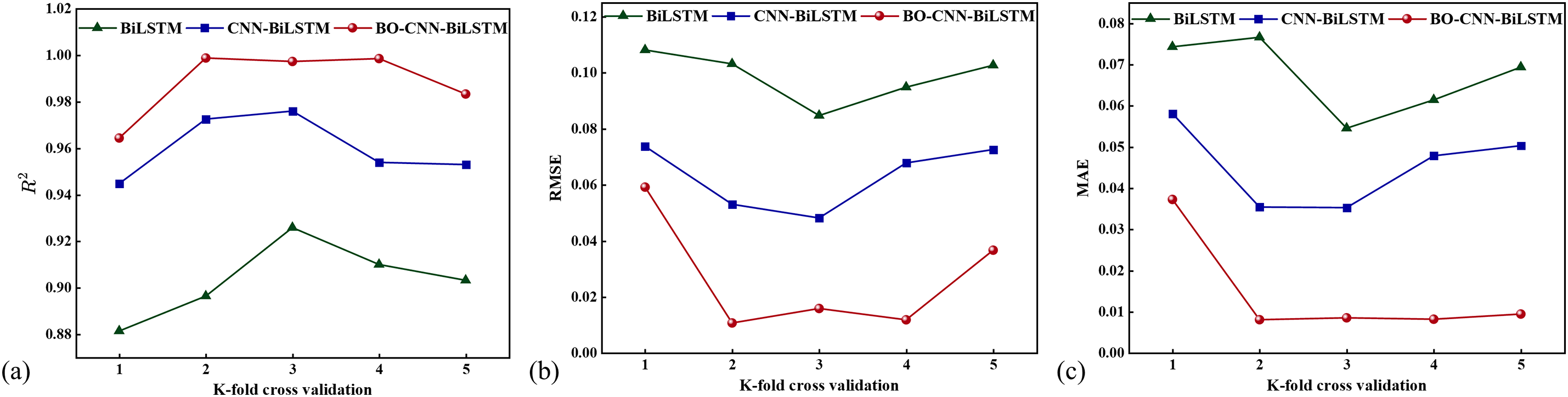
Figure 6: The prediction results of the model under K-fold cross-validation, including: (a) Correlation Coefficient (R2), (b) Root Mean Square Error (RMSE), and (c) Mean Absolute Error (MAE)
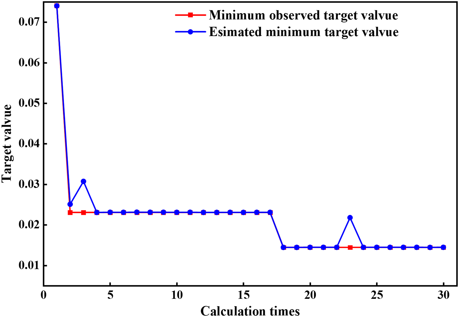
Figure 7: Optimize iteration curve
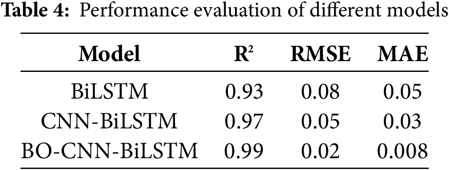
In order to compare the performance of different models more intuitively, Fig. 8 shows the scatter plot of the test set. From the figure, it can be seen that combining CNN and BiLSTM can fully extract the data features while considering the time-series data relationships. Compared with BiLSTM, the prediction accuracy of CNN-BiLSTM is improved from 0.93 to 0.97. The prediction accuracy of the model can be further improved by optimizing the hyperparameters using BO, and the optimized model prediction accuracy is improved from 0.97 to 0.99. The above analysis shows that the proposed BO-CNN-BiLSTM model has higher prediction accuracy and more concentrated fitting distribution.
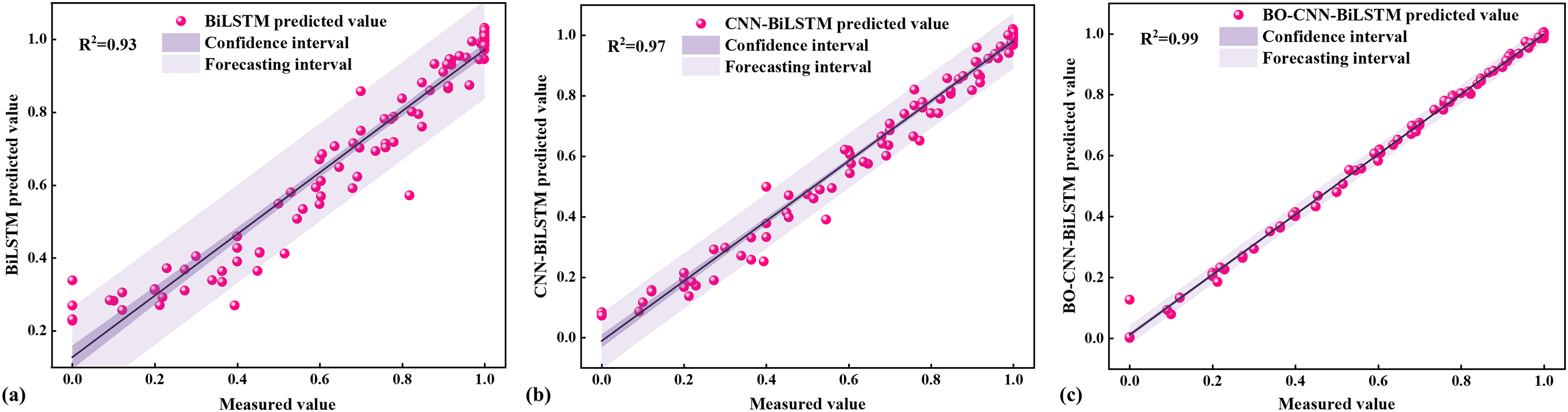
Figure 8: Comparison of prediction accuracy of different models: (a) Prediction results of BiLSTM, (b) Prediction results of CNN-BiLSTM, and (c) Prediction results of BO-CNN-BiLSTM
In this study, a fatigue life prediction method for composites based on the BO-CNN-BiLSTM model was proposed, which combines the advantages of the CNN and BiLSTM models, and optimizes the hyperparameters of the hybrid neural network using the Bayesian optimization algorithm to improve the model accuracy and reliability. Redundant features were eliminated through covariance analysis, and features closely related to fatigue damage were extracted, and boundary conditions were incorporated into the feature data using unique thermal coding to form a high-quality sample library; the BO-CNN-BiLSTM fatigue life prediction model was constructed, and the automatic tuning of the model hyper-parameters was achieved through the Bayesian optimization algorithm, which further improves the predictive performance of the model. The prediction results of BiLSTM, CNN-BiLSTM and BO-CNN-BiLSTM models were compared through experimental validation. The experimental results show that:
Compared with the other two models, the proposed BO-CNN-BiLSTM model has higher accuracy, less dispersion of prediction results, and shows higher reliability in the prediction task. Specifically, the BO-CNN-BiLSTM model demonstrates superior performance in all metrics when compared to the CNN-BiLSTM model. The R2 of BO-CNN-BiLSTM is 2% higher than that of CNN-BiLSTM. The root mean square error (RMSE) is reduced to 0.02, and the mean absolute error (MAE) is reduced to 0.008. Despite the evident enhancements in prediction accuracy and model reliability, it must be acknowledged that the present study is not without its limitations. The model’s efficacy is contingent upon the utilization of a particular dataset, and its performance may be subject to variation when applied to disparate types of composite materials or other operational environments. Subsequent research endeavors will involve the execution of transfer learning tests on a more extensive array of datasets, with the objective of enhancing the model’s generalizability.
In summary, the present study proposes a promising method for predicting life in composite materials caused by fatigue. This method has the potential to be applied in the aerospace, automotive, and civil engineering sectors. Subsequent advancements in data diversity, real-time adaptability, and model scalability are anticipated to further augment the model’s effectiveness and reliability in complex engineering systems.
Acknowledgement: Not applicable.
Funding Statement: This research was funded by the Key Technologies R&D Program of CNBM (2023SJYL01), Postgraduate Research & Practice Innovation Program of Jiangsu Province (SJCX24_1356).
Author Contributions: The authors confirm contribution to the paper as follows: study conception and design: Mengke Ding, Dongyue Gao, Jun Li, Zhanjun Wu; data collection: Mengke Ding, Borui Wang, Guotai Zhou; analysis and interpretation of results: Mengke Ding, Dongyue Gao, Jun Li; draft manuscript preparation: Mengke Ding. All authors reviewed the results and approved the final version of the manuscript.
Availability of Data and Materials: Data openly available in a public repository. The data that support the findings of this study are openly available in https://www.nasa.gov/intelligent-systems-division/discovery-and-systems-health/pcoe/pcoe-data-set-repository/ (accessed on 14 July 2025).
Ethics Approval: Not applicable.
Conflicts of Interest: The authors declare no conflicts of interest to report regarding the present study.
References
1. Bjorheim F, Siriwardane SC, Pavlou D. A review of fatigue damage detection and measurement techniques. Int J Fatigue. 2022;154(8):106556. doi:10.1016/j.ijfatigue.2021.106556. [Google Scholar] [CrossRef]
2. Shiri S, Pourgol-Mohammad M, Yazdani M. Probabilistic assessment of fatigue life in fiber reinforced composites. In: Proceedings of the ASME, 2014 International Mechanical Engineering Congress and Exposition; 2014 Nov 14–20; QC, Canada. V014T08A018. [Google Scholar]
3. Lai J, Xia Y, Huang Z, Liu B, Mo M, Yu J. Fatigue life prediction method of carbon fiber-reinforced composites. e-Polymers. 2024;24(1):20230150. doi:10.1515/epoly-2023-0150. [Google Scholar] [CrossRef]
4. Dong F, Li Y, Li B. Acoustic emission-driven fatigue damage evolution equation and life prediction of composite laminates. Int J Fatigue. 2025;198(2):109012. doi:10.1016/j.ijfatigue.2025.109012. [Google Scholar] [CrossRef]
5. Jin HS, Yan JJ, Liu X, Li WB, Qing XL. Quantitative defect inspection in the curved composite structure using the modified probabilistic tomography algorithm and fusion of damage index. Ultrasonics. 2021;113:106358. doi:10.1016/j.ultras.2021.106358. [Google Scholar] [PubMed] [CrossRef]
6. Gharehbaghi VR, Noroozinejad Farsangi E, Noori M, Yang TY, Li S, Nguyen A, et al. A critical review on structural health monitoring: definitions, methods, and perspectives. Arch Comput Methods Eng. 2022;29(4):2209–35. doi:10.1007/s11831-021-09665-9. [Google Scholar] [CrossRef]
7. Qing XL, Liao YL, Wang YH, Chen BQ, Zhang FH, Wang YS. Machine learning based quantitative damage monitoring of composite structure. Int J Smart Nano Mater. 2022;13(2):167–202. doi:10.1080/19475411.2022.2054878. [Google Scholar] [CrossRef]
8. Goyal D, Pabla BS. The vibration monitoring methods and signal processing techniques for structural health monitoring: a review. Arch Comput Methods Eng. 2016;23(4):585–94. doi:10.1007/s11831-015-9145-0. [Google Scholar] [CrossRef]
9. Qing XL, Li WZ, Wang YS, Sun H. Piezoelectric transducer-based structural health monitoring for aircraft applications. Sensors. 2019;19(3):545. doi:10.3390/s19030545. [Google Scholar] [PubMed] [CrossRef]
10. Sharma A, Mukhopadhyay T, Rangappa SM, Siengchin S, Kushvaha V. Advances in computational intelligence of polymer composite materials: machine learning assisted modeling, analysis and design. Arch Comput Methods Eng. 2022;29(5):3341–85. doi:10.21203/rs.3.rs-471723/v1. [Google Scholar] [CrossRef]
11. Jung KC, Chang SH. Advanced deep learning model-based impact characterization method for composite laminates. Compos Sci Technol. 2021;207(2):108713. doi:10.1016/j.compscitech.2021.108713. [Google Scholar] [CrossRef]
12. Ju M, Dou ZS, Li JW, Qiu XT, Shen BL, Zhang DW, et al. Piezoelectric materials and sensors for structural health monitoring: fundamental aspects, current status, and future perspectives. Sensors. 2023;23(1):543. doi:10.3390/s23010543. [Google Scholar] [PubMed] [CrossRef]
13. Fan XY, Li J, Hao H. Review of piezoelectric impedance based structural health monitoring: physics-based and data-driven methods. Adv Struct Eng. 2021;24(16):3609–26. doi:10.1177/13694332211038444. [Google Scholar] [CrossRef]
14. Na WS, Baek J. A review of the piezoelectric electromechanical impedance based structural health monitoring technique for engineering structures. Sensors. 2018;18(5):1307. doi:10.3390/s18051307. [Google Scholar] [PubMed] [CrossRef]
15. Zhao GQ, Wang B, Wang T, Hao WF, Luo Y. Detection and monitoring of delamination in composite laminates using ultrasonic guided wave. Compos Struct. 2019;225:111161. doi:10.1016/j.compstruct.2019.111161. [Google Scholar] [CrossRef]
16. Nasir V, Ayanleye S, Kazemirad S, Sassani F, Adamopoulos S. Acoustic emission monitoring of wood materials and timber structures: a critical review. Constr Build Mater. 2022;350(9):128877. doi:10.1016/j.conbuildmat.2022.128877. [Google Scholar] [CrossRef]
17. Sha F, Xu DY, Cheng X, Huang SF. Mechanical sensing properties of embedded smart piezoelectric sensor for structural health monitoring of concrete. Res Nondestruct Eval. 2021;32(2):88–112. doi:10.1080/09349847.2021.1887418. [Google Scholar] [CrossRef]
18. Kulakovskyi A, Mesnil O, Chapuis B, D’Almeida O, Lhémery A. Statistical analysis of guided wave imaging algorithms performance illustrated by a simple structural health monitoring configuration. J Nondestruct Eval Diagn Progn Eng Syst. 2021;4(3):031001. doi:10.1115/1.4049571. [Google Scholar] [CrossRef]
19. Yue N, Aliabadi MH. Hierarchical approach for uncertainty quantification and reliability assessment of guided wave-based structural health monitoring. Struct Health Monit. 2020;20(5):2274–99. doi:10.1177/1475921720940642. [Google Scholar] [CrossRef]
20. Deng SZ, Zhou J. Prediction of remaining useful life of aero-engines based on CNN-LSTM-Attention. Int J Comput Intell Syst. 2024;17(1):232. doi:10.1007/s44196-024-00639-w. [Google Scholar] [CrossRef]
21. Mirzaei AH, Haghi P, Shokrieh MM. Prediction of fatigue life of laminated composites by integrating artificial neural network model and non-dominated sorting genetic algorithm. Int J Fatigue. 2024;188(4):108528. doi:10.1016/j.ijfatigue.2024.108528. [Google Scholar] [CrossRef]
22. Mizuno Y, Hosoi A, Koshita H, Tsunoda D, Kawada H. Fatigue life prediction of composite materials using strain distribution images and a deep convolution neural network. Sci Rep. 2024;14(1):25418. doi:10.1038/s41598-024-75884-2. [Google Scholar] [PubMed] [CrossRef]
23. Song R, Sun L, Gao Y, Peng C, Wu X, Lv S, et al. Global-local feature cross-fusion network for ultrasonic guided wave-based damage localization in composite structures. Sens Actuators A Phys. 2023;362(4):114659. doi:10.1016/j.sna.2023.114659. [Google Scholar] [CrossRef]
24. Wang J, Li X, Li J, Sun Q, Wang H. NGCU: a new RNN model for time-series data prediction. Big Data Res. 2022;27(8):100296. doi:10.1016/j.bdr.2021.100296. [Google Scholar] [CrossRef]
25. Shakhovska N, Shymanskyi V, Prymachenko M. FractalNet-LSTM model for time series forecasting. Cmes-Comput Model Eng Sci. 2025;82(3):4469–84. doi:10.32604/cmc.2025.062675. [Google Scholar] [CrossRef]
26. Ariafar S, Coll-Font J, Brooks D, Dy J. ADMMBO: bayesian optimization with unknown constraints using ADMM. J Mach Learn Res. 2019;20(123):1–26. [Google Scholar]
27. Li XF, Guo HA, Xu LX, Xing ZZ. Bayesian-based hyperparameter optimization of 1D-CNN for structural anomaly detection. Sensors. 2023;23(11):50. doi:10.3390/s23115058. [Google Scholar] [PubMed] [CrossRef]
28. Saxena A, Goebel K, Larrosa CC, Janapati V, Roy S, Chang FK. Accelerated aging experiments for prognostics of damage growth in composite materials [Internet]. [cited 2025 Jul 14]. Available from: https://c3.ndc.nasa.gov/dashlink/static/media/publication/2011_IWSHM_Composites.pdf. [Google Scholar]
29. Zhang FT, Zhang KF, Cheng H, Gao DY, Cai KY. Fatigue damage monitoring of composite structures based on lamb wave propagation and multi-feature fusion. J Compos Sci. 2024;8(10):423. doi:10.3390/jcs8100423. [Google Scholar] [CrossRef]
30. Yuan SF, Wang H, Chen J. A PZT based on-line updated guided wave-gaussian process method for crack evaluation. IEEE Sens J. 2020;20(15):8204–12. doi:10.1109/jsen.2019.2960408. [Google Scholar] [CrossRef]
31. Zhang FT, Zhang KF, Cheng H, Gao DY, Cai KY. Ultrasonic guided wave health monitoring of high-temperature aircraft structures based on variational mode decomposition and fuzzy entropy. Actuators. 2024;13(10):411. doi:10.3390/act13100411. [Google Scholar] [CrossRef]
32. Liang X. Image-based post-disaster inspection of reinforced concrete bridge systems using deep learning with Bayesian optimization. Comput-Aided Civ Infrastruct Eng. 2019;34(5):415–30. doi:10.1111/mice.12425. [Google Scholar] [CrossRef]
Cite This Article
 Copyright © 2025 The Author(s). Published by Tech Science Press.
This work is licensed under a Creative Commons Attribution 4.0 International License , which permits unrestricted use, distribution, and reproduction in any medium, provided the original work is properly cited.
 Downloads
 Citation Tools