Heuristic Weight Initialization for Transfer Learning in Classification Problems

1  Introduction

Utilizing knowledge acquired in one domain to facilitate learning in another domain is known as Transfer Learning (TL). This approach does not rely on assumptions about training and test data’s independence and identical distribution. TL also offers a solution to challenges such as limited data availability [1] and constraints on computational resources [2] when training models in a new domain. This method is primarily employed for transferring knowledge across closely related domains [1–4], not consistently yielding superior results [1,4], called ‘negative transfer.’ Even when domains are related, TL can have adverse effects if pre-trained models lack transferable and beneficial components from the domains [2,4]. Nonetheless, reference [5] demonstrated recently that TL can also be applied across entirely distinct domains. For example, a language corpus-trained model could be applied to offline reinforcement learning.

Authors in [2] reviewed over 50 research studies in the area of TL within Deep Neural Networks (DNNs) and classified the methods into four primary categories regarding solutions: model-based, discrepancy-based, Generative Adversarial Network (GAN)-based, and relational-based approaches. However, researchers commonly categorize traditional TL in Machine Learning into four types: 1. instance, 2. feature, 3. parameter, and 4. relational-based approaches [1]. The advent of DNNs allowed traditional methods to be applied to unstructured data, leveraging features extracted by convolutional neural networks (CNNs). Additionally, modern NNs, largely reliant on backpropagation, also called “vanilla” NNs, use a variety of loss functions, including Maximum Mean Discrepancy [6], Gumbel softmax distribution [7,8].

Retraining models with various hyperparameters called fine-tuning, particularly preserving similarities between domains with residual networks, representing discrete values with categorical [7], showed better generalization at the early stage of DNN. However, reference [9] later reported that it has certain limitations across datasets when applied to segmentation problems. To address this limitation, weakly supervised learning is utilized to generate pseudo-labels [10]. Additionally, other approaches have emerged in tandem, including transformer-based methods [11] and dual-stream architectures [12].

Before the widespread adoption of Deep Neural Network (DNN) models, traditional techniques, notably highlighted by [13] in image processing and Computer Vision, relied on filters to extract features from images for the construction of Machine Learning (ML) models. Reference [14] empirically demonstrated that specific filters are constructed in the early layers of CNNs. They concluded that the first layer is not dependent on specific tasks or datasets. Subsequently, reference [15] extended the previous findings through extensive numerical experiments. They recommended extracting all layers from pre-trained models, except for the last classification layer, to adapt these models to new domains.

In this work, we develop a linear classifier model relying upon the conclusion above and the logistic regression model by [16,17] in which the weights are expressed in two terms and computed heuristically. Our proposal differs from existing work significantly. For example, weight initialization techniques principally aim to trade-off between gradient vanishing and exploding [9,18] since these methods initialize whether entirely or partially model from randomly generated values, the initial model’s accuracy is 100/C, where C is a number of classes. Another track of existing work relied on gradient-based weighting [19,20] also has several well-known issues, including a requirement on an extra model or several iterations detailed in the next section, that is not fitted to our setting. Precisely, we apply these results to TL for classification problems leveraging features extracted from DNN models and illustrate our results in various tasks and settings. Specifically, we utilize CNNs, ViTransformers for image and audio classification, and BERT models for text classification as feature extractors, considering datasets have fewer classes since many practical datasets have small sets of classes [21,22]. Additionally, our target is to transfer learned knowledge in practical tasks requiring fewer examples. Lastly, The structure of the remainder of this work is as follows: the next section provides a description and comparison of existing works, followed by an elaboration of the proposed approach in the third section. The empirical outcomes and discussions are presented in the last two sections.

2  Related Work

Existing research can be divided into two sections according to the approach being proposed: TL overviewed in the last section in DNN architectures and computing weights for a logistic model. The latter problem is solved widely by gradient descent approaches, and it is also very well known. And we also assume that we have extracted features from DNN models. Therefore, we mainly describe methods that find weights of a linear model heuristically rather than gradient descent. Nonetheless, when applying TL on the same architecture, it’s common practice to initialize the weights with random values, following the same strategy used for training most NN models. References [23,24] introduced random weight initialization methods, coupled with variates, to enhance the flow of backpropagation and improve the convergence of gradient optimization algorithms. However, despite these advancements, these methods do not always improve model performance.

Several gradient-based weight initialization methods have been proposed to address the challenges of vanishing and exploding gradients. Layer-Sequential Unit-Variance (LSUV) Initialization [19] iteratively adjusts weight scaling using forward passes until activations reach unit variance, achieving stable gradient propagation. However, its iterative nature incurs an additional complexity of O(niterkd), where niter is the number of forward passes needed to stabilize activations, k and d are number of input and output features, respectively. Fixup Initialization [18] was introduced as an alternative specifically for deep residual networks, eliminating the need for Batch Normalization by applying learned scaling factors to each layer. This method maintains an O(kd) complexity but relies on specific architectural constraints, assuming the presence of residual connections. MetaInit [20] explores meta-learning techniques to optimize initialization, leveraging gradient information from a preliminary training phase. Despite its effectiveness in adapting initialization to different tasks, its computational cost is significantly higher at O(Tkd), where T represents the number of meta-training steps. HyperInitialization uses hypernetworks to generate weight initialization dynamically, introducing additional overhead proportional to the hypernetwork size H. While these methods offer improved stability over traditional statistical initializations, they often rely on strong assumptions, such as well-conditioned gradient distributions or the availability of meta-training data, which may limit their applicability in resource-constrained settings. As our best knowledge, none of them explicitly considers our setting.

As the approach basises sorting values of a given feature, it requires average O(nlogn). To avoid this problem, we use smaller subsets as much as possible, such as 64, 128, etc. The next part is a number of out features we need to also take into account, so overall complexity is O(knlogn), where k is feature dimension and n is example size. While some of the above-mentioned methods assume an extra model or residual connections, the rest usually train the model over some iterations. To conclude, our setting is to compute the weights of the newly added fully connected layers with a small amount of data in which most existing work does not fit.

Let’s denote the dataset of examples with X={x1,x2,…,xM}, where xi∈RN and yi∈{0,1} is the target value for instance xi∈XN. Additionally, Kl denotes a set of instances whose target is equal to l, and |Kl| is the number of examples in class l. Now, let’s consider the following traditional logistic regression model for xi∈X:

y^=∑j=1Nwjxji=w⋅xi(1)

where wj∈RN are learnable parameters of the model 1. This model is formulated differently by [16] as a combination of two learnable variables of the weights and two summations for numerical and categorical features considered independently as follows:

y^=∑j∈Itjwjxji+∑j∈Jtjwjxji(2)

where tj∈{−1,1}, wj∈[0,1], I, and J are class order indicators, weights, a quantitative feature set, and a qualitative feature set, respectively. The authors normalized numerical features into interval [−1,1] and calculated probabilities for each category in feature j conditioning on target values as in preprocessing stages. This specific model allows them to constrain possible parameters w from continuous as the former model has multiple solutions [25] to discrete variables if weights w in the later model are computed deterministically. Nevertheless, finding optimal values of tj∈{−1,1} still is NP-complete with 2N combinations. This limitation is later solved by [17] under a strict rule that assumes each class object objects are located in two intervals. If this assumption is held, then tj=1, otherwise tj=−1. This paper also utilizes the final model to address multiclassification problems using a one-vs.-all approach, employing different heuristics to determine the models’ weights.

These heuristics from Information Gain, including the GINI index and Entropy, are widely used to build Decision Tree models. Traditional decision trees mainly split continuous variables into partitions for some natural reasons [26]; however, this approach lacks extracted features. Reference [26] introduces a parameter, proposing a hybrid approach incorporating continuous features into conventional decision trees. Additionally, with these heuristics, we show that our approach can have comparable accuracies by only using a small subset of datasets, such as 64 or 128. Also, we do not train models using gradient-based approaches such as Adam and SGD (Stochastic Gradient Descent).

3  Proposed Method

As the proposed method solely computes the weights for the final classifier layer, and our objective involves transfer learning, we can presume the existence of a predetermined feature extractor, as depicted in Fig. 1. The feature extractor transforms unstructured data into tabular or tabular data, which we utilize to identify the local optimal solution in classification tasks. In the subsequent subsections, we assume we are working with tabular data to define the present problem. Hence, we avoid using notations associated with transfer learning, such as denoting source or target domains and tasks.

Figure 1: A common feature extractor for unstructured data. However, since the proposed method is designed specifically for tabular data, it calculates weights for the final fully connected layer

3.1 Notations and Problem Statement

Let’s consider multiclassification problem notations above and also denoting target values by yi∈{0,1,…,K} for instance xi∈X, where K is the number of classes. Additionally, Kl denotes a set of instances whose target is equal to l, and |Kl| is the number of examples in class l. Now, let’s consider the following linear model for one instance with K outputs for each class, analogous to the final classifier layers in NN models for object xi∈X.

y^=xi⋅(t⊙w)(3)

where t, w are N×K matrices to represent class orders with entities tij={−1,1} and weights with entities wj∈[0,1] for each feature, respectively, and ⊙ element-wise multiplication. Given that each output of the head layer utilizes the same data with different weights, we can extend its application to multiclassification problems by employing the “one vs. all” approach. This technique, commonly used in various well-known ML models such as softmax in NN [27] or by combining K binary classifiers in SVM (Support Vector Machine) [28], enables us to address multiclassification tasks. In this work, our task is to compute the above parameters of the model in Eq. (3) using these heuristics.

3.2 Computing Heuristic Weights

Initializing DNN models with non-zero (but not close to zero) constant values can result in gradient exploding, whereas initializing with values close to zero or zeros can lead to gradient vanishing or not learning. To avoid these issues, references [23,24] proposed random initialization techniques with normal distribution as a function of weight dimensions and variance; even multiplication with 0.5 leads to earlier convergence in larger models. Therefore, we propose to use the class orders with a constant value as follows, assuming given (extracted) tabular data correlated with targets. The motivation behind the idea is illustrated in Table 1 as a simple binary classification with 15 synthetic instances described by three inputs and one target, consisting of 9 and 6 samples for the first and second classes. Entries in the dataset are generated from a uniform distribution with range [0, 0.7] and [0.3, 1] for the classes and features 1 and 3, respectively, and the distribution range for feature two is purposely reversed regarding classes. Simply adding these 3-feature values might lead a linear classifier to be less accurate with constant weights for each feature, whereas multiplying 2-feature values by −1 improves the linear separability of the space, producing accuracies of 0.67±0.12 and 0.91±0.09 on 10,000 repetitions accordingly. A recently published paper also suggests a matrix quantization on LLM (Large Language Model) to convert 16-bit weights to 1-bit by representing these entities into {−1,0,1} [29]. The most crucial problem is to obtain these values for each feature since there are many suboptimal solutions even with class orders, as we do not know each feature order. For example, while we choose w=(1−11) in the experiment, w=(1−11) is also feasible, but reversing class outputs. In this subsection, we provide and develop three heuristics to resolve deterministic class orders and weights for each feature, only independently learning conditional probabilities of features on target values. However, Gaussian Mixture Models and gradient descent techniques usually consider feature correlations [30], which often leads to superior performance.

The key underlying idea of computing these parameters is to divide sorted feature values into two disjoint intervals for each class. To implement this, we first sort the given feature values and then search for the optimal border of the intervals regarding specific measurements, which will be explained later. The search process involves all possible binary divisions of these values while guaranteeing that each interval must have one value at least. This process is feasible since we leverage a small subset of training examples. Otherwise, other approaches may be better as sorting has a significant time complexity with O(mnlog(n)), where m and n are the numbers of samples and extracted features, respectively. Let’s denote the numbers of the first and second-class examples in the first and second intervals by U∈{0∪N}2×2. Algorithm 1 outlies finding a weight only for variable xj conditioned on target y, where function measurement is defined later. We also use indexing [index] along with subscripts and superscripts.

To measure the separability of the divisions, we leverage three heuristics: entropy and the GINI index from Information Gain widely used in decision trees and the last is introduced in [16]. As the first two criteria are leveraged in many applications by researchers, we only include the third one as shown in Eq. (4). The first two criteria can only be applied to the conditioning of categorical variables on the target. Continuous variables are usually divided into bins before feeding them. In this case, we use them in the binary division of output values of DNN models, but unlike bins, the division is found by Algorithm 1 to maximize the heuristic value.

measure(U)=(∑d=12∑i=12Uid(Uid−1)∑i=12|Ki|(|Ki|−1))(∑d=12∑i=12Uid(|K3−i|−U3−id)2|K1||K2|)(4)

where the values of the first and second braces indicate the similarity and difference of the two classes by the underlying feature conditioning on target y. The measurement value lies in range [0,1], and if it is equal to 1, then two class objects are located in two intervals without mixing.

Once we’ve established the boundary using either described heuristics, we can ascertain the class order tj for feature j. In general, one straightforward solution to compute this value is to know where the target class object values are located, whether mostly on the left or right side of certain output sorted values. If most of these values are higher than others, then we assign +1. Otherwise, we can just assign −1. But, another possible case in which they may be mixed with others might prevent getting the exact better value. So, we only compute it regarding the border deterministically found by explained heuristics. If we have the border values dividing the sorted values into two intervals, we use Algorithm 2 to determine it. The typical problem of the One verse All approach is the first class values are fewer than that of the second. This raises the class-imbalance challenge, which is also taken into account by Algorithm 2, computing relative probabilities over corresponding class sizes and internals.

3.3 Theoretical Background

Suppose binary classification and first-class objects are located in the first interval to not consider the class direction in this analysis. Traditional linear classifiers assign equal weight to all features, which may lead to overfitting when irrelevant or weakly predictive features dominate. To mitigate this issue, we use a feature-weighting scheme based on heuristic purities, where the contribution of each feature is scaled according to its discriminative power [31]. We define the transformed feature representation as a weighted sum of features, where the weights are given by one of the purity values:

Z=∑j=1dP(Xj)Xj.(5)

This transformation enhances the impact of highly pure features while suppressing the influence of less informative ones. The resulting classifier operates in the modified feature space Z, which is expected to improve generalization by reducing the model’s susceptibility to noise [25]. We consider the Rademacher complexity to analyze the generalization performance, which provides an upper bound on the expected error. For a linear classifier fW(X)=WTX, the empirical Rademacher complexity is given by:

ℛ^(ℱ)≤|W|2Rn,(6)

where R is the maximum norm of the input feature vectors and n is the number of samples [32]. When applying the heuristic weighting, the transformed feature norm of (5) is modified as:

|Z|22=∑j=1dP(Xj)2|Xj|22.(7)

Thus, by substituting (7) into (6), the Rademacher complexity of the weighted classifier becomes:

ℛ^(ℱP)≤|W|2n(∑j=1dP(Xj)2Rj2)1/2,(8)

where Rj is the maximum norm of each feature; since lower-purity features contribute less, this bound is effectively reduced, leading to better generalization performance. Furthermore, using results from VC-dimension theory, the generalization error of a linear classifier in a d-dimensional space is given by:

E[error]≤error^+O(dlog⁡nn).(9)

By weighting features according to the heuristic weights, the effective dimension is reduced to d~=O(k), where k is the number of dominant features. This yields an improved bound:

E[error]≤error^+O(klog⁡nn).(10)

Since k≪d in most cases, this result suggests that heuristic-based feature weighting enhances generalization by effectively regularizing the classifier [33]. Our theoretical analysis demonstrates that incorporating the heuristic weighting into the feature representation improves generalization by reducing Rademacher complexity and the practical VC dimension. This method offers a principled approach to feature selection that prioritizes highly informative features while suppressing noise.

3.4 Analysis of Heuristics

We first compare GINI and Entropy since the difference between them is only log function. Let’s denote binary class probabilities in the left interval by p1 and p2 and define GINI and Entropy by G(p1,p2)=1−p12−p22 and H(p1,p2)=−p1log⁡(p1)−p2log⁡(p2), respectively. Both functions reachs their maximum values (0.5 and 1) when the class distribution is uniform, p1=p2=0.5, that is the most impurity1. For these two heuristics, we can easily obtain the following property and inequality: both heuristics are monotonic (purity reaches its maximum value of 1); G(p1,p2)≥H(p1,p2). For proofs, refer to [30,31,34]. They show that for any split, the GINI Index will result in less impurity than the Entropy measure, meaning that the GINI Index leads to a more aggressive split when the problem is class imbalance. In other words, as we often leverage the one-vs.-all approach that leads to class imbalance problems naturally, so we may prefer Entropy over GINI Index. Given a split by matrix U∈{0∪N}2×2, we need to consider the purity of classes in each interval and also to be fair with Eq. (4) since it deems both sides statistics, we next define more appropriate versions of these heuristics by PG(U)=G(q1,q2)−n1nG(p11,p21)−n2nG(p12,p22) and PH(U)=H(q1,q2)−n1nH(p11,p21)−n2nH(p12,p22), where qi=|Ki|n, nj=U1j+U2j, and pij=Uijnj, respectively. The first terms coincide with the total impurity of two classes that, if the dataset is totally balanced, their values are equal 0.5 and 1. In contrast, the last two terms express the purity of each interval, respectively. Most importantly, these two purity heuristics require more examples due to reversely associating with n while Eq. (4) does not. The empirical also approves this statement in Fig. 2. Additionally, the alternatives are more conservative than Eq. (4), which leads to zero weights in the worst-case scenarios. For example, suppose a split given by matrix U=(4646), then both alternatives equal to 0 while Eq. (4) is 0.22 since the later always mix two internal statistics in both its term while the alternatives consider separately. From Section 3.3, we obtained the improved bound (10) that the smaller k the smaller expected error. Nevertheless, we witness empirically that more zero-weights leads to loss more information in Section 4. Additionally, we can conclude the same for the complexity relying (8) that the alternatives may lead less complexity bound, but we empirically find Nikolay’s heuristic is much better as we explained above.

Figure 2: Results of 8 random experiments, accuracies generally increase with larger subsets, but not drastically. Note: annotations are given repeatedly with various heuristics while omitting base model names

4  Experimental Results

As the proposed approach assumes that its input is tabular, we can apply it to various data types, such as images, texts, and audio, in the context of model-based transfer learning problems. To illustrate results in more settings, we use various-sized subsets from training sets to compute weights. Table 2 depicts a fragment of outcomes (other results are located in Appendix C, the source code repository) for several datasets from 3 domains with different pre-trained models from Kaggle2. As mentioned earlier, we only add one classifier layer to CNN models for image classification tasks and calculate its weights heuristically. In text classification problems, the input from feature extractors is pooled output of the pre-trained models (BERT models and their various modifications [35]) in related domains. The CNN pre-trained models used in classification problems are also employed to classify audio signals by creating their spectrograms, multiplying their channel by 3, as CNN models only consume three channels. Furthermore, we also consider binary classification as two output NN models since these two terms are equal [30].

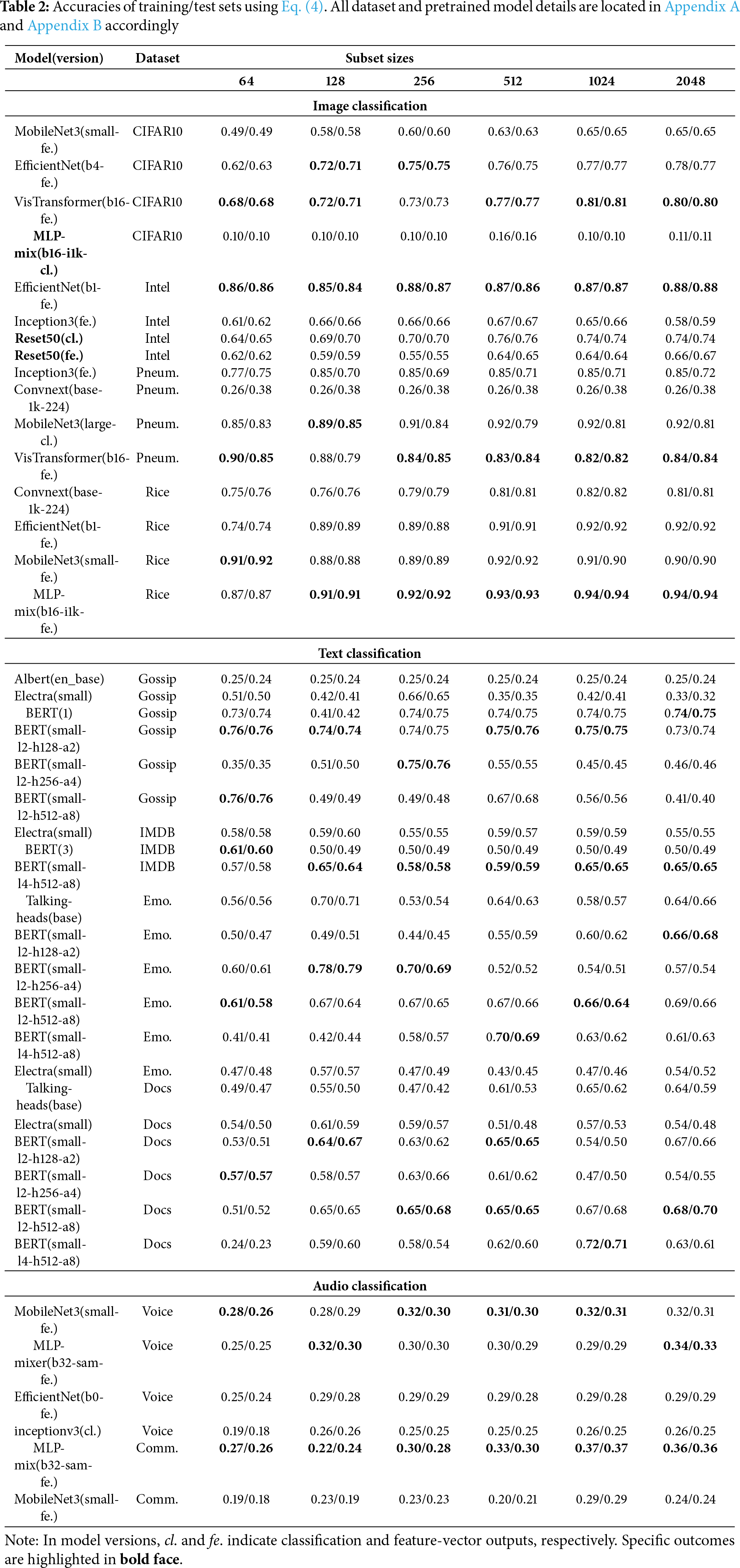
When we apply the proposed method to the head layer of pre-trained models in image classification, the results dropped significantly compared to feature extractor layers as concluded in [14,15] except ResNet50. Particularly, this phenomenon can be seen in almost all outcomes of MLP-mixers, for example, 10%, which is the random guessing value on CIFAR10. The most suitable reason, we think, for the MLP-mixer on CIFAR10 with classification output is that its architecture does not have convolutional layers [36]. Another notable wonder is witnessed after assigning heuristic weights to the head layer; that is, further training models on these weights is always worse than training with random parameters applying gradient descent optimizations. Reference [9] also concluded a similar case that fine-tuning pre-trained models does not always produce better results and suggested self-training models.

As subset sizes increase, accuracies also increase in mostly image and audio datasets with few exceptions as we sample subsets randomly. This trend cannot encountered in the rest. Instead, the higher results are located in subsets with sizes 128, 256, and 512. Nevertheless, this trend often goes up significantly in smaller subsets, and later changes in accuracies are not remarkable, as shown in Fig. 2. This might conclude that the proposed method can be used with smaller subsets by providing sufficient samples for each class. For example, MobileNet3 on 64 Rice samples classified 92% of objects correctly while EfficientNet achieved 86% on Intel images just 2% less than the highest. Additionally, training and test accuracies are almost equal on large datasets compared to the training subset number, for example, CIFAR10, but not Pneum. since we trained models from a small subset of samples. Finally, when it comes to text classification tasks, models with fewer parameters tend to outperform larger models. However, meticulously training these larger models does not necessarily lead to significant improvements in their performance. This leads to the conclusion that a small set of datasets is sufficient to compute the weights.

As Table 2 depicts outcomes for only Eq. (4), we generalize respective results of the GINI index and entropy by comparing with Eq. (4) in Fig. 3 to provide a more comprehensive understanding. Since the number of total experiments is 145 and subsets are drawn randomly, Fig. 3 illustrates how frequently each measurement outperformed the other alternatives across different subset sizes. Computing weights in Eqs. (3) by (4) surpasses 5 out of 6. For the smallest subset size of 64, metric nikolay has the highest score of 76, followed by entropy at 31 and GINI at 38. As the subset size increases, the variation in the performance of the metrics shrinks. However, the average absolute differences between Nikolay with entropy and GINI and entropy with GINI are roughly 4.86%, 4.62%, and 2.68%, respectively.

Figure 3: 145 experiments, demonstrating that Nikolay’s weight-based approach outperformances 5 out of 6

5  Discussion and Conclusion

The paper introduces a heuristic approach as an alternative to backpropagation methods for computing the weights of a newly added layer in neural networks when performing transfer learning. Although backpropagation methods are generally superior and outperform the proposed approach, we suggest using their method as an initialization technique. Despite being outperformed by conventional methods in most cases, the proposed heuristic approach sometimes produces results very close to those obtained through backpropagation, but with the advantage of using only a small subset of the training data. Therefore, we present the method as a computationally efficient way to initialize the weights of new layers in transfer learning scenarios, which can be further fine-tuned using conventional backpropagation techniques. We observe almost the same accuracies in text datasets with gradient-decent-based algorithms.

This method involves combining multiple problems in the initial phases. In the context of AutoML model selection, it can be utilized to first select models before hyperparameter tuning, aiming to reduce the number of potential models for a specific task. When introducing a new class to the output layer, we can also utilize it by simply obtaining a small subset of examples, likewise, few-shot learning, upon which the approach calculates the weights. The approach can also be advantageous for semi-supervised learning, as it necessitates only a small number of examples.

We also experimented with the approach in various configurations, but unfortunately, the outcomes were unsatisfactory. One approach involves selectively truncating certain features for each class output independently. The most straightforward implementation is to utilize a threshold parameter to assign zero weights to those features. The configuration leads to a significant decrease in accuracy. We then implemented the feature ranking method described in [17], but unfortunately, it did not yield improved results. We can add more other fields in our approach that can be more beneficial than other settings. For example, Federated learning requires keeping model architecture in each device separately and running models that do not require intensive computing resources.

Limitations. This heuristic approach possesses several notable limitations, primarily due to its lack of reliance on theoretical analysis. One of them is further training heuristically weighted models that cannot outperform their randomly initialized counterparties. However, according to the conclusion of [9], this flaw is inherent to the proposed approach. Another limitation arises when the number of classes is large, leading to computational challenges requiring samples and computing weights from extracted features for each class. Nevertheless, the experiments involve outcomes for CIFAR100, showing roughly 33% on 1024 examples. This limitation can be avoidable when specific samples are drawn for each class separately. Lastly, the last dataset is the Audio classification problem in which we first created audio spectrograms as an image, which is an out-domain dataset since the original CNN model is trained on ImageNet. Therefore, the results are not so desirable to compare with full gradient-based transfer learning. One mitigation solution will be to directly use the same domain-trained models, which extract better feature representations of datasets.

Directions for future work. Several directions could be given to improve the approach’s findings along with a range of applications in related domains. Firstly, the limitations, including regression problems, larger classes, efficiency, etc., should be mitigated to enhance this approach’s applicability in other domains. Secondly, whether the annealing this approach or not, many safety-first domains should be considered to be improvements. For example, safety in Reinforcement learning is most important. Suppose we have a small expert dataset since acquiring a large dataset is not feasible in practice to train an RL (Reinforcement Learning) agent. If we use existing methods, they give random guesses or require more samples. Another example could be federated learning settings where local models must be trained locally on a few examples.

Acknowledgement: Not applicable.

Funding Statement: This study was supported by the BK21 FOUR project (AI-driven Convergence Software Education Research Program) funded by the Ministry of Education, School of Computer Science and Engineering, Kyungpook National University, Republic of Korea (4120240214871). This work was also supported by the New Faculty Start Up Fund from LSU Health Sciences New Orleans, LA, USA.

Author Contributions: The authors confirm contribution to the paper as follows: Conceptualization, methodology, software, validation, formal analysis, Musulmon Lolaev; resources, Anand Paul; writing—original draft preparation, writing—review and editing, visualization, Musulmon Lolaev; supervision, Anand Paul and Jeonghong Kim. All authors reviewed the results and approved the final version of the manuscript.

Availability of Data and Materials: Data openly available in a public repository. The data that support the findings of this study are openly available in the UCI Machine Learning Repository at https://archive.ics.uci.edu/ (accessed on 08 June 2025).

Ethics Approval: Not applicable.

Conflicts of Interest: The authors declare no conflicts of interest to report regarding the present study.

Appendix A

All datasets are publicly available as listed in Table A1.

Appendix B Pretrained Models

All pre-trained models from Kaggle are detailed in Table A2.

Appendix C All Results

We leveraged all models in Table A2 over datasets in Table A1, so all results are stored in files, folder ‘res-log’ of https://anonymous.4open.science/r/transfer-learning-D46C (accessed on 08 June 2025) as reporting in the paper requires so much space. This repository contains all source code, experiments, and their reports in the paper. To reproduce outcomes, please read the readme file.

1As we consider only one interval, so P1+P2=1 is not necessarily.

2All models are trained and published by Google, formerly TensorFlowHub. CNN and VisTransformer models are pre-trained on ImageNet, while BERT models are on various datasets.

References

1. Panigrahi S, Nanda A, Swarnkar T. A survey on transfer learning. In: Intelligent and cloud computing. Singapore: Springer; 2021. p. 781–9. doi:10.1007/978-981-15-5971-6_83. [Google Scholar] [CrossRef]

2. Yu F, Xiu X, Li Y. A survey on deep transfer learning and beyond. Mathematics. 2022;10(19):3619. doi:10.3390/math10193619. [Google Scholar] [CrossRef]

3. Joseph S, Parthi AG, Maruthavanan D, Jayaram V, Veerapaneni PK, Parlapalli V. Transfer learning in natural language processing. In: 2024 7th International Conference on Information and Communications Technology (ICOIACT); 2024 Nov 20–21; Ishikawa, Japan. p. 30–6. doi:10.1109/ICOIACT64819.2024.10912895. [Google Scholar] [CrossRef]

4. Zhuang F, Qi Z, Duan K, Xi D, Zhu Y, Zhu H, et al. A comprehensive survey on transfer learning. Proc IEEE. 2021;109(1):43–76. doi:10.1109/JPROC.2020.3004555. [Google Scholar] [CrossRef]

5. Reid M, Yamada Y, Gu SS. Can Wikipedia help offline reinforcement learning? arXiv:2201.12122. 2022. [Google Scholar]

6. Rozantsev A, Salzmann M, Fua PV. Beyond sharing weights for deep domain adaptation. IEEE Trans Pattern Anal Mach Intell. 2016;41:801–14. doi:10.1109/TPAMI.2018.2814042. [Google Scholar] [PubMed] [CrossRef]

7. Jang E, Gu S, Poole B. Categorical reparametrization with Gumble-Softmax. In: 5th International Conference on Learning Representations, ICLR 2017; 2017 Apr 24–26; Toulon, France. [Google Scholar]

8. Potapczynski A, Loaiza-Ganem G, Cunningham JP. Invertible Gaussian reparameterization: revisiting the gumbel-softmax. Vol. 33. Red Hook, NY, USA: Curran Associates, Inc.; 2020. p. 12311–21. doi:10.5555/3495724.3496756. [Google Scholar] [CrossRef]

9. He K, Girshick RB, Dollár P. Rethinking ImageNet pre-training. In: 2019 IEEE/CVF International Conference on Computer Vision (ICCV); 2019 Oct 27–Nov 2; Seoul, Republic of Korea. p. 4917–26. doi:10.1109/ICCV.2019.00502. [Google Scholar] [CrossRef]

10. Xie Q, Luong MT, Hovy E, Le QV. Self-training with noisy student improves ImageNet classification. In: 2020 IEEE/CVF Conference on Computer Vision and Pattern Recognition (CVPR); 2020 Jun 13–19. Seattle, WA, USA. p. 10684–95. doi:10.1109/CVPR42600.2020.01070. [Google Scholar] [CrossRef]

11. Dosovitskiy A, Beyer L, Kolesnikov A, Weissenborn D, Zhai X, Unterthiner T, et al. An image is worth 16 × 16 Words: transformers for image recognition at scale. arXiv: 2010.11929. 2021. [Google Scholar]

12. Ghifary M, Kleijn W, Zhang M. Domain adaptive neural networks for object recognition. In: The 13th Pacific Rim International Conference on Artificial Intelligence; 2014 Dec 1–5; Gold Coast, QLD, Australia. p. 898–904. doi:10.1007/978-3-319-13560-1_76. [Google Scholar] [CrossRef]

13. Krizhevsky A, Sutskever I, Hinton EG. Imagenet classification with deep convolutional neural networks. In: Advances in neural information processing systems. Cambridge, MA, USA: MIT Press; 2012. p. 1097–105. doi:10.1145/3065386. [Google Scholar] [CrossRef]

14. Yosinski J, Clune J, Bengio Y, Lipson H. How transferable are features in deep neural networks?. In: Proceedings of the 27th International Conference on Neural Information Processing Systems-Volume 2, NIPS’14. Cambridge, MA, USA: MIT Press; 2014. p. 3320–8. doi:10.5555/2969033.2969197. [Google Scholar] [CrossRef]

15. Chu B, Madhavan V, Beijbom O, Hoffman J, Darrell T. Best practices for fine-tuning visual classifiers to new domains. In: Computer Vision–ECCV 2016 Workshops (ECCV 2016). Cham, Switzerland: Springer; 2016. p. 435–42. doi:10.1007/978-3-319-49409-8_34. [Google Scholar] [CrossRef]

16. Nikolay I. Computing generalized parameters and data mining. Autom Remote Control. 2011;72:1068–74. doi:10.1134/S0005117911050146. [Google Scholar] [CrossRef]

17. Musulmon L, Naik SM, Paul A, Chehri A. Heuristic weight initialization for diagnosing heart diseases using feature ranking. Technologies. 2023;11(5):138. doi:10.3390/technologies11050138. [Google Scholar] [CrossRef]

18. Zhang H, Dauphin YN, Ma T. Fixup initialization: residual learning without normalization. In: 7th International Conference on Learning Representations, ICLR 2019; 2019 May 6–9; New Orleans, LA, USA. [Google Scholar]

19. Mishkin D, Matas J. All you need is a good init. In: Proceedings of the 2015 International Conference on Computer Vision (ICCV); 2015 Dec 7–13; Santiago, Chile. p. 1316–24. [Google Scholar]

20. Dauphin YN, Bengio Y. MetaInit: initializing learning by learning to initialize. In: Proceedings of the Advances in Neural Information Processing Systems (NeurIPS); 2019 Dec 8–14; Vancouver, BC, Canada. p. 3159–70. doi:10.5555/3454287.3455420. [Google Scholar] [CrossRef]

21. Hendrycks D, Basart S, Mu N, Kadavath S, Wang F, Dorundo E, et al. The many faces of robustness: a critical analysis of out-of-distribution generalization. In: 2021 IEEE/CVF International Conference on Computer Vision (ICCV). 2021 Oct 10–17; Montreal, QC, Canada. p. 8320–9. doi:10.1109/ICCV48922.2021.00823. [Google Scholar] [CrossRef]

22. Sun C, Shrivastava A, Singh S, Gupta AK. Revisiting unreasonable effectiveness of data in deep learning era. In: 2017 IEEE International Conference on Computer Vision (ICCV). 2017 Oct 22–29; Venice, Italy. p. 843–52. doi:10.1109/ICCV.2017.97. [Google Scholar] [CrossRef]

23. Glorot X, Bengio Y. Understanding the difficulty of training deep feedforward neural networks. In: Proceedings of the 13th International Conference on Artificial Intelligence and Statistics (AISTATS) 2010; 2010 May 13–15. Sardinia, Italy. p. 249–56. [Google Scholar]

24. He K, Zhang X, Ren S, Sun J. Delving deep into rectifiers: surpassing human-level performance on ImageNet classification. In: 2015 IEEE International Conference on Computer Vision (ICCV). 2015 Dec 7–13; Santiago, Chile. p. 1026–34. doi:10.1109/ICCV.2015.123. [Google Scholar] [CrossRef]

25. Hastie T, Tibshirani R, Friedman J. The elements of statistical learning: data mining, inference, and prediction. Cham, Switzerland: Springer Science & Business Media; 2009. [Google Scholar]

26. Negi A, Sharma S, Priyadarshini J. Gini index and entropy-based evaluation: a retrospective study and proposal of evaluation method for image segmentation. Singapore: Springer; 2020. p. 239–48. doi:10.1007/978-981-15-2854-5_22. [Google Scholar] [CrossRef]

27. Bridle JS. Probabilistic interpretation of feedforward classification network outputs, with relationships to statistical pattern recognition. In: Soulié FF, Hérault J, editors. Neurocomputing. Berlin/Heidelberg, Germany: Springer; 1990. p. 227–36. doi:10.1007/978-3-642-76153-9_28. [Google Scholar] [CrossRef]

28. Hsu CW, Lin CJ. A comparison of methods for multiclass support vector machines. IEEE Trans Neural Netw. 2002;13(2):415–25. doi:10.1109/72.991427. [Google Scholar] [PubMed] [CrossRef]

29. Ma S, Wang H, Ma L, Wang L, Wang W, Huang S, et al. The era of 1-bit LLMs: all large language models are in 1.58 bits. arXiv:2402.17764. 2024. [Google Scholar]

30. Bishop CM. Pattern recognition and machine learning (Information science and statistics). 1st ed. Berlin/Heidelberg, Germany: Springer; 2007. [Google Scholar]

31. Breiman L, Friedman JH, Olshen RA, Stone CJ. Classification and regression trees. 1st ed. Boca Raton, FL, USA: Chapman and Hall/CRC; 1984. doi:10.1201/9781315139470. [Google Scholar] [CrossRef]

32. Bartlett PL, Mendelson S. Rademacher and Gaussian complexities: risk bounds and structural results. J Mach Learn Res. 2002;3:463–82. doi:10.5555/944919.944944. [Google Scholar] [CrossRef]

33. Vapnik VN. Statistical learning theory. Hoboken, NJ, USA: John Wiley & Sons, Inc.; 1998. doi:10.1007/978-1-4757-3264-1. [Google Scholar] [CrossRef]

34. Quinlan JR. Induction of decision trees. Mach Learn. 2004;1:81–106. doi:10.1007/BF00116251. [Google Scholar] [CrossRef]

35. Devlin J, Chang MW, Lee K, Toutanova K. BERT: pre-training of deep bidirectional transformers for language understanding. In: Proceedings of the 2019 Conference of the North American Chapter of the Association for Computational Linguistics: Human Language Technologies; 2019 Jun 2–7; Minneapolis, MN, USA. p. 4171–86. doi:10.18653/v1/N19-1423. [Google Scholar] [CrossRef]

36. Tolstikhin IO, Houlsby N, Kolesnikov A, Beyer L, Zhai X, Unterthiner T, et al. MLP-Mixer: an all-MLP architecture for vision. In: NIPS’21: Proceedings of the 35th International Conference on Neural Information Processing Systems; 2021 Dec 6–14; Online. p. 24261–72. doi:10.5555/3540261.3542118. [Google Scholar] [CrossRef]