
 Submit a Paper
 Propose a Special lssue
 Open Access
ARTICLE
Research on Fault Probability Based on Hamming Weight in Fault Injection Attack
Department of Information Security, Naval University of Engineering, Wuhan, 430000, China
* Corresponding Author: Tong Wu. Email:
Computers, Materials & Continua 2025, 85(2), 3067-3094. https://doi.org/10.32604/cmc.2025.066525
Received 10 April 2025; Accepted 08 July 2025; Issue published 23 September 2025
 View Full Text
 Download PDF
Abstract
Fault attacks have emerged as an increasingly effective approach for integrated circuit security attacks due to their short execution time and minimal data requirement. However, the lack of a unified leakage model remains a critical challenge, as existing methods often rely on algorithm-specific details or prior knowledge of plaintexts and intermediate values. This paper proposes the Fault Probability Model based on Hamming Weight (FPHW) to address this. This novel statistical framework quantifies fault attacks by solely analyzing the statistical response of the target device, eliminating the need for attack algorithm details or implementation specifics. Building on this model, a Fault Injection Attack method based on Mutual Information (FPMIA) is introduced, which recovers keys by leveraging the mutual information between measured fault probability traces and simulated leakage derived from Hamming weight, reducing data requirements by at least 44% compared to the existing Mutual Information Analysis method while achieving a high correlation coefficient of 0.9403 between measured and modeled fault probabilities. Experimental validation on an AES-128 implementation via a Microcontroller Unit demonstrates that FPHW accurately captures the data dependence of fault probability and FPMIA achieves efficient key recovery with robust noise tolerance, establishing a unified and efficient framework that surpasses traditional methods in terms of generality, data efficiency, and practical applicability.Keywords
Fault attacks usually introduce precise and controllable faults that affect the regular operation of the target device, change its program flow and logic state, and obtain information about the key. Injected faults usually include clock [1], voltage [2], laser [3], electromagnetic faults [4,5] and other types. Due to its strong attack capability, short attack time, fewer analysis data, and no need for expensive equipment [6], fault injection has gradually become a more effective method for integrated circuit security attacks.
Recently, many fault attack methods have been proposed based on different types of faults. Li et al. [7] proposed Fault Sensitivity Analysis, which constantly changes the intensity of injection faults to observe the threshold of fault ciphertext. Ghalaty et al. [8] proposed Differential Fault Intensity Analysis to analyze the change of fault ciphertext with fault intensity. Dobraunig et al. [9] proposed Statistical Ineffective Fault Analysis to examine the invalid fault, which does not affect the encryption operation after injection. Ghalaty et al. [8] proposed Blind Fault Analysis to analyze the Hamming Weight (HW) of the intermediate value of two consecutive rounds of encryption. The above methods must master the specific plaintext, ciphertext, or intermediate value data. They are related to the particular implementation form of the algorithm, so they are unsuitable for all fault attacks.
Saha et al. [10] proposed the Fault Template Attack, which traverses all the keys and constructs the template after fault injection. Still, the calculation of the template construction process is too complex. Spruyt et al. [11] The proposed Fault Correlation Analysis (FCA) converts the power traces into fault probability traces, which qualitatively verifies the correlation between fault probability and power consumption but does not quantitatively analyze the statistical characteristics of fault probability.
When describing the relationship between the state change and the leakage information during the operation of the cryptographic algorithm of the target equipment, side-channel attacks usually explain the leakage information through the leakage models, such as Hamming Weight model [12,13], Hamming Distance (HD) model [14], Gaussian model [15,16]. From the point of view of information theory, fault attacks quantify security through information entropy [17], mutual information [18], and so on. However, most leakage models of fault attacks are aimed at specific scenarios or countermeasures, so they are not universal.
The leakage model is an essential tool for fault attack assessment, and its accuracy will affect the reliability of the evaluation. Currently, most leakage models of fault attacks have limitations, such as not simultaneously considering the data requirements, data volume, fault tolerance, and attack efficiency. Constructing a unified leakage model of fault attacks can not only profile all attacks uniformly but also reduce the requirement for the amount of data and noise interference.
To establish a leakage model to describe fault attacks uniformly, a Fault Probability model based on Hamming Weight (FPHW) is proposed and studied in this paper. Based on the AES algorithm of the MCU, the fault attack is carried out, and the operation dependence and data dependence of fault probability are verified and analyzed. Then, a fault injection attack method based on the FPHW model from the perspective of mutual information (FPMIA) is proposed, which can recover key bytes by the mutual information between the measured and the simulated leakage with 28 fault probability traces.
The article is organized as follows: In Section 2, the FPHW model is established, the operation and data dependence of fault probability are analyzed macroscopically, and the principle of FPMIA is described. Section 3 introduces the method of fault attack in detail. Section 4 verifies the proposed model and its performance by analyzing and evaluating the experimental response. Section 5 describes the design and implementation of the FPMIA method. Finally, Section 6 concludes this article.
FCA puts forward the approach of categorizing the responses from target equipment. The method involves the simultaneous repeated injection of operation-related faults to determine the probability of each fault type at a specific time point. The probability that a fault response may occur at each sampling point is defined as the fault probability of the sampling point. If this process is repeated at different time points, the fault probability trace of the whole operation process can be obtained.
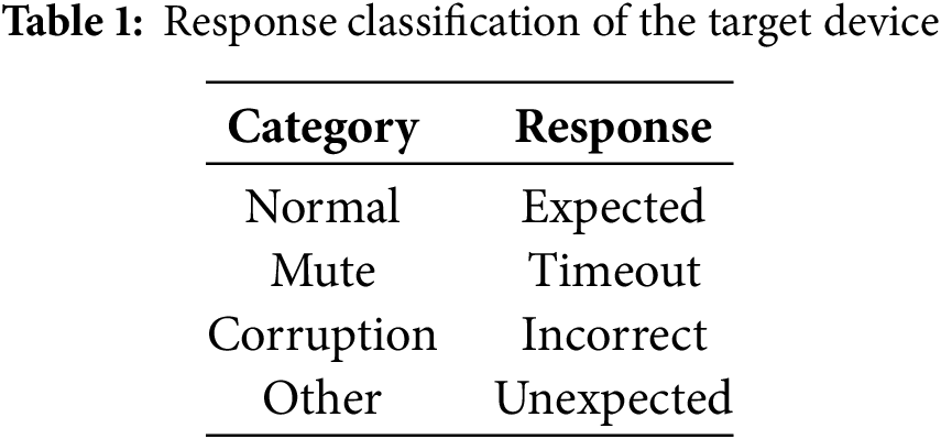
In this study, the fault probability model classifies the target device’s response into four types: standard, mute, corruption, and other, as shown in Table 1.
In this paper, we choose a model based on corruption probability to observe whether the device returns an incorrect response. Fault attacks based on fault probability exploit the probability of a cryptographic device failing depends on the operations performed and the data the device processes. This is also why the fault probability trace is subdivided into operation-dependent and data-dependent components. We have structured the fault probability model using the relevant principles of power analysis attacks [19]. It is assumed that the probability of the target device depends on the operations being performed and the data being processed by the device. For each point on the fault probability traces, the operation-dependent component is denoted as FPop, and the data-dependent component is denoted as FPdata. In addition, the influence of the instability of the target device and the fault source on the fault probability is denoted as FPel.noise. Therefore, the fault probability of each point on the fault probability trace is denoted as Eq. (1). The change of FPop and FPdata mainly causes the numerical fluctuation of FPtotal. Therefore, an attacker can obtain key information by analyzing FPop and FPdata.
2.2 Operation Dependence of Fault Probability
During the fault injection attack process, the response distribution changes with the glitch depth and width, as shown in Fig. 1. As the depth and width of the glitch increase, the attack energy gradually increases. The response of the target device gradually transitions from “normal” to “corruption” “mute” and “other”.
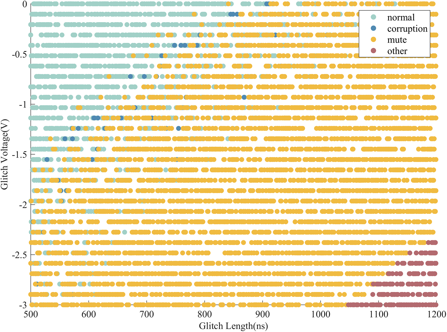
Figure 1: Distribution of responses in the whole process of attack
Fig. 2 shows the responses for each time slice, where the x-axis represents the glitch length and the y-axis represents the glitch voltage. The scattered points in the figure indicate the device’s response under corresponding glitch lengths and voltages. Blue means “corruption” responses, and green indicates other responses. Due to the different operations performed at each moment, the response distribution also changes accordingly. There are apparent differences in the distribution of various responses with varying depths of glitch and widths. It means that the fault probability is related to the operation at each moment and has operation dependence.
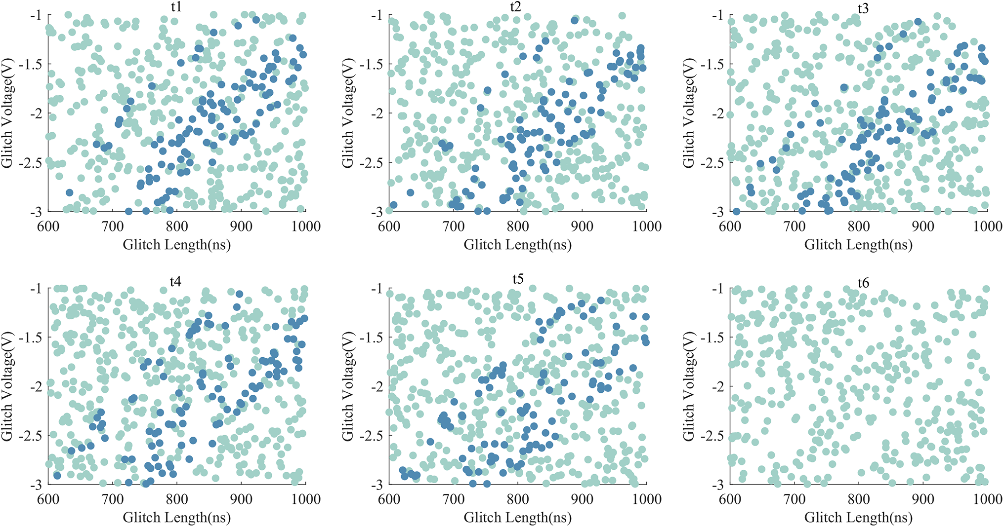
Figure 2: Distribution of responses at different times
During the experiment, it can be observed that the response after fault injection is distributed in a centralized manner. Curves can be fitted at the intersection of different responses. The curvature, inflection point, and asymptote of the curve contain relevant information about data, operations and fault sensitivity. Since this paper focuses on the data dependence of fault probability, the operational dependence needs to be analyzed in depth here.
2.3 Data Dependence of Fault Probability
After conducting numerous fault injections, it is noted that there is a significant difference in the fault probability for data of different HW. Since fault probability has specific data dependence, and the probability of 0→1 and 1→0 may differ, we build a fault probability model based on HW, rather than the HD model.
Define the probability of single-bit 0→1 transition as P0, 1→0 transition as P1, and the fault probability of single-byte data due to bit flipping is:
In information theory and probability theory, the mutual information (MI) of two random variables indicates the degree of interdependence of the variables. In general, the MI of two discrete variables X and Y is defined as Eq. (3), where p(x, y) is the joint probability distribution function of X and Y, and p(x) and p(y) are the marginal probability distribution functions of X and Y, respectively.
MI quantifies the information we can grasp about one variable X while observing another variable Y. In evaluating side-channel security, we can use MI to quantify how much we can learn about keys when observing the physical leakage of target devices. The amount of MI can also be used to judge the quality of the leakage model. The model effect is better if the simulated leakage is closer to the measured leakage.
This paper proposes the FPMIA method based on the FPHW model, and the principles of FPMIA are as follows. For a fixed time t, the operation being performed by the target cryptographic device is represented as a function f. The plaintext is denoted as p, the key is denoted as k, the leakage function is denoted as L, and the linear coefficient is denoted as a, then for time t, Eq. (1) can be rewritten as:
To evaluate the leakage amount of cryptographic equipment, we use Eq. (5) to assess the MI between simulated and measured leakage. If the simulated leakage value is expressed as L and the measured leakage value is expressed as FP, the MI between them is:
Since p(fp, l) cannot be calculated, it can be rewritten as follows:
Substitute Eq. (6) into Eq. (5) to get:
The measured fault probabilities are classified according to the FPHW model, and the probability distribution p(fp) is estimated. The simulated fault probabilities are classified according to the HW model, and the probability distribution p(l) is estimated. The measured leakage samples are divided into groups according to the simulated leakage, and their probability distribution p(fp|l) is estimated. The greater the MI between the simulated and measured leakage, the greater the physical leakage of the cryptographic device.
3 Exploration Methods for Data Dependence of Fault Probability
Firstly, the attacker model employed in this paper is outlined as follows. An attacker can transmit arbitrary plaintexts and observe the output of any S-box. Additionally, the attacker can access the responses generated by the cryptographic device. Rather than measuring the specific data outputted by the S-box alone, this paper emphasizes measuring the device’s overall response. However, it is essential to note that the ciphertext and the key remain inaccessible to the attacker.
This paper takes the AES-128 algorithm as a case study to examine the data dependence concerning fault probability. We carry out numerous fault injection attacks on the output of the first S-box during the initial round of encryption. The specific analysis process is shown in Fig. 3.
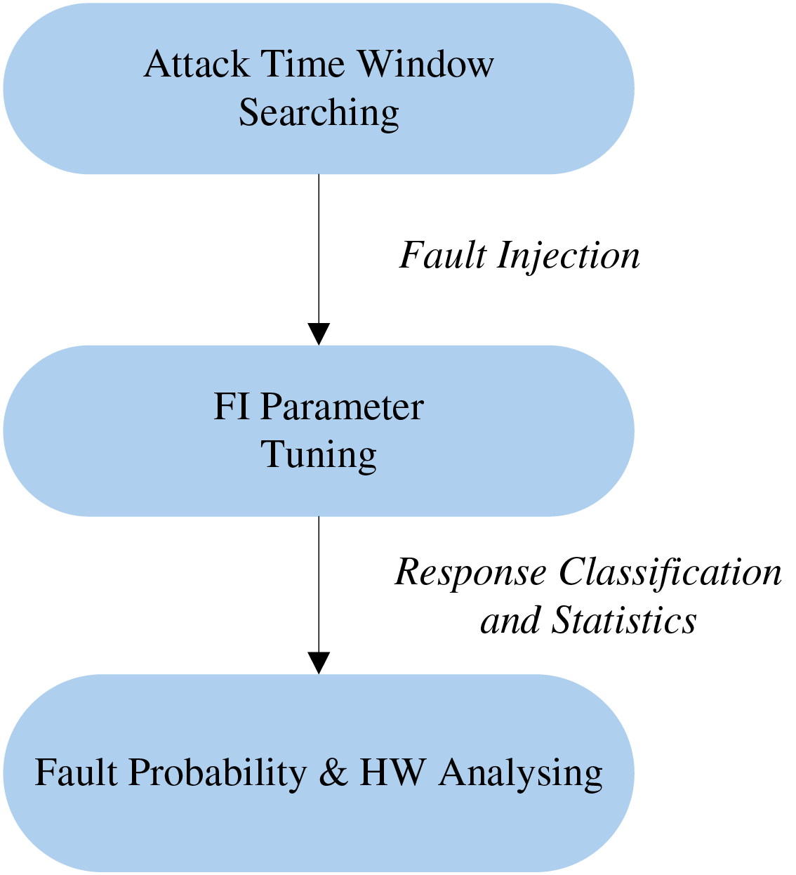
Figure 3: Attack flow
The steps of fault injection attacks and data analysis based on FPHW are as follows:
• Step 1: Choose the time window for the attack. Perform multiple Correlation Power Analysis (CPA) on AES-128 encryption to analyze the leakage point of the 1st S-box output in the first round of encryption.
• Step 2: Choose effective fault injection parameters. Using a wide range of random parameters to inject many glitches in the time window determined in Step 1. Then, narrow the parameters until the response results within each time slice of the time window to have an approximate mix of 50% “corruption” and 50% others.
• Step 3: Perform fault injection attacks. For 256 plaintexts with different HW whose first byte is different and the rest are the same, use the selected fault injection parameters to inject voltage glitches within the time window and record the device response. Establish fault probability traces and analyze the fault probability at each moment.
4 Effectiveness Verification of the FPHW Model
The general structure of the experimental attack platform is illustrated in Fig. 4a, primarily comprising the attack target, fault injection controller, oscilloscope monitoring module, and data acquisition-processing module. The cryptographic target of the attack is the DMCU-F405, which employs an STM32F405RGT6 MCU as its microcontroller. The fault injection controller contains a glitch creation module and a current boosting module, supplying parameters like pulse delay, glitch voltage, glitch duration, and baseline level to the MCU. Under specified pulse delays, these modules can generate glitches of any duration.
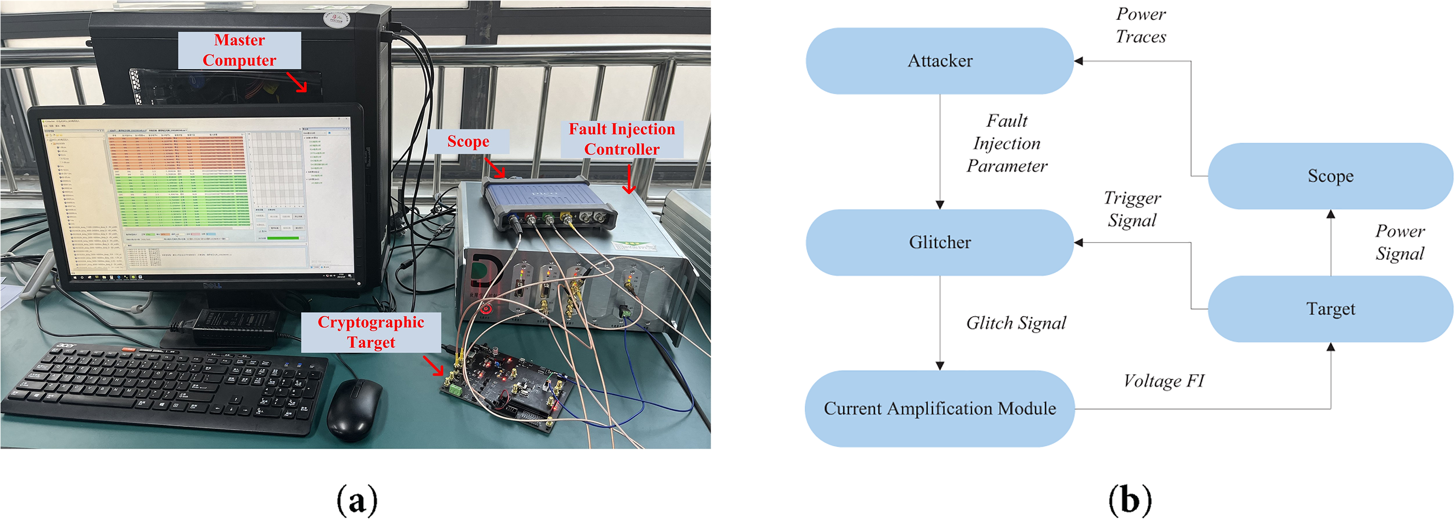
Figure 4: Voltage glitch injection experiment: (a) Experimental site; (b) Experimental schematic diagram
Fig. 4b depicts the experimental schematic layout. The PC side uses Attacker software to constantly transmit plaintext, which the attack target encrypts upon receipt and sends the ciphertext back to the PC for storage. Initially, the fault injection controller processes the trigger signal from the MCU development board during encryption-decryption operations to generate a glitch signal. Subsequently, the current amplification module converts this glitch signal into the voltage glitch required for fault attacks. Lastly, the attack on the MCU cryptographic target involves injecting these voltage glitches for fault induction.
Perform multiple CPAs on AES-128 to find the leakage point of the first S-box output of the first round of encryption. Experimental results show that the leakage peak is about 12,000 ns. Combined with the operation instructions near the leak point, through the calculation of the instruction cycle, the time window is judged as a delay of 8000 to 16,000 ns.
Many voltage glitches of different lengths and voltages are injected into the time window. The fault probability traces of the five plaintexts in the time window are shown in Fig. 5. The x-axis delay represents the pulse delay provided by the fault injection controller to the MCU, which is the delay time between the injected glitch and the trigger signal. Fig. 5 demonstrates that the fault probability for specific data segments remains 0 across certain time intervals, signifying that voltage glitches do not influence the first S-box operation during the initial encryption round. This implies an inaccuracy in the time window configuration. Through tuning and analysis, it was found that the glitch activation timing is slightly delayed relative to the input timing. To ensure glitches can impact the first-round first S-box operation, a delay is inserted before the operation, with glitch injection executed within this delayed interval.
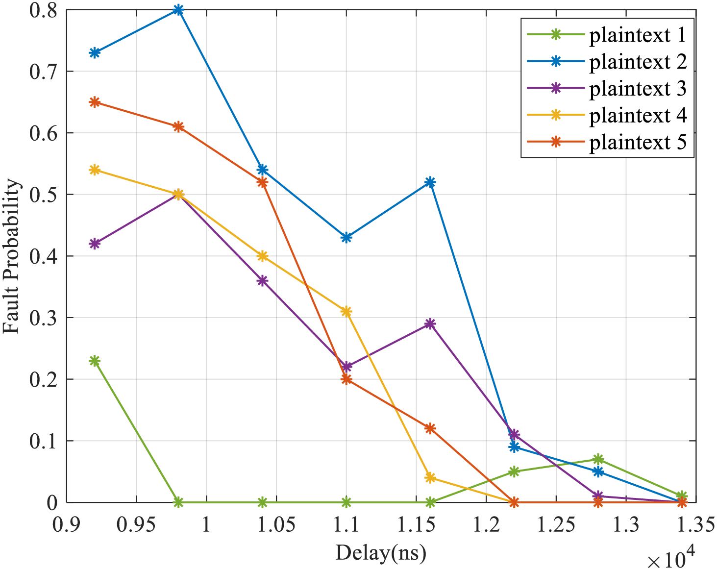
Figure 5: Fault probability traces of 5 plaintexts
Fig. 6 shows the waveform diagram following the addition of trigger signals. Initially, the experiment introduces a trigger signal prior to the S-box operation instruction, referred to as a “small trigger” signal. A trigger signal is added within several microseconds before the small trigger, known as a “large trigger” signal. A glitch is injected between the large and small trigger signals to guarantee that the glitch can impact the S-box operation. Many voltage glitches are injected between the two trigger signals, and the target device seldom responds with “corruption” outside the delay range of 880~900 ns. Therefore, the delay window of the attack is 880~900 ns.
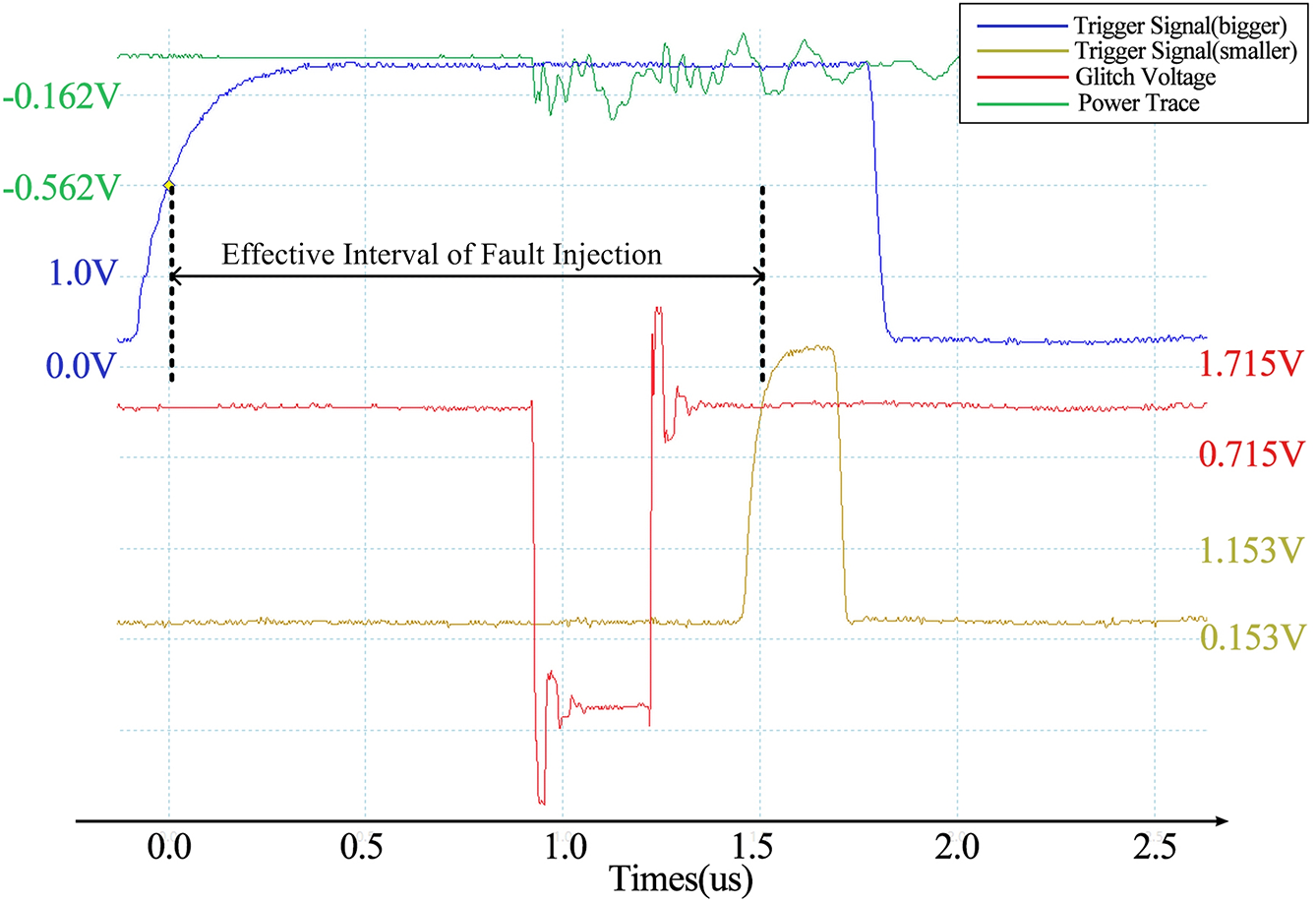
Figure 6: Glitch waveform under trigger signals
Within the time window determined above, we choose a voltage range from 0 V to the extremum (−6 V). The length ranges from hundreds to thousands of nanoseconds to inject many glitches. Fault injection parameters are selected incrementally to identify the suitable range, aiming to make the proportion of “corruption” responses in the results of each time slice within the time window around 50%.
The approach for determining these fault injection parameters follows a progressive narrowing strategy:
• Step 1: Initial Scanning: Randomly inject faults within a wide range (glitch depth: 0 to −6 V, width: 100 to 3000 ns), and record the response distribution of each time slice.
• Step 2: Interval Shrinkage: For each time slice, select parameter intervals with a “corruption” response rate close to 50% using parameter stepping (e.g., voltage step of 0.1 V, length step of 50 ns), and exclude extreme response regions.
• Step 3: Fine Adjustment: Inject faults within the shrunk interval with smaller steps (voltage: 0.01 V, length: 1 ns) and determine the optimal parameter combination through the bisection method to stabilize the “corruption” response rate of each time slice at 45%–55%.
Fig. 7 shows the response distribution of each slice in the time window. The green represents “corruption” responses, the red represents other responses, and the square boxes represent the fault parameter intervals that meet the requirements.
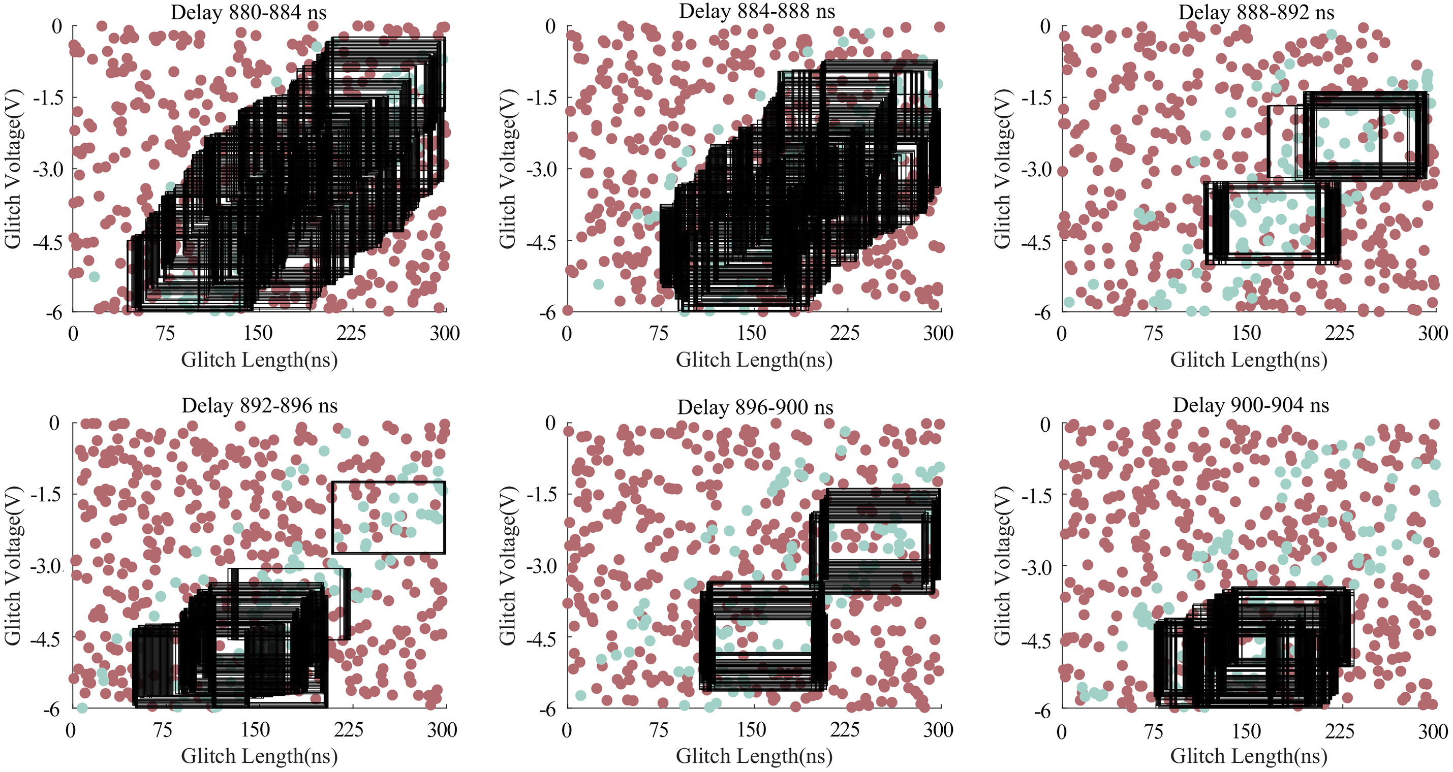
Figure 7: Response distribution and effective interval selection in each time slice
It can be seen from Fig. 7 that the effective interval is roughly distributed at the intersection of the two types of responses. The larger the parameter interval setting and the larger the step, the fewer possible effective intervals in each time slice. Generally, it does not affect the selection of effective intervals in the entire attack window. The size of the parameter interval and step length will impact the choice of effective parameter intervals, as will the number of attacks per time slice. We only need to select a suitable set of fault injection parameters. The selection results of the effective intervals in the three groups of tests are shown in Table 2.
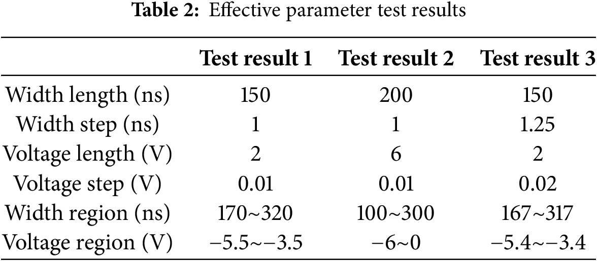
Eventually, the fault injection parameters chosen for the attack feature a glitch width ranging from 100 to 300 ns and a voltage spanning from −6 to 0 V.
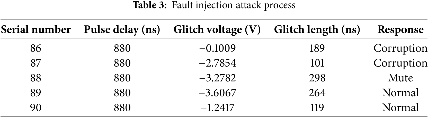
Next, select the above parameters to inject many faults in the time window, as shown in Table 3. Given that the attack target is the output of the first S-box in the initial round of AES-128 encryption, our focus remains solely on the first byte of the ciphertext generated by the S-box output. The 256 possibilities output by the first S-box are classified according to the HW, and 256 plaintexts are obtained by inverse operation. For each of the 256 plaintexts, use the fault injection parameters in the effective interval to attack 1000 times, record the fault response of each data in each time slice, and establish 256 fault probability traces.
To determine the probability distribution of the fault probability of the target device when processing different data, we performed a dependence analysis of the fault probability on the data. The distribution of FPdata is related to the target device and the distribution of the processed data. In every subsequent discussion, it is presumed that the processed data follow a uniform distribution pattern. This means that all values appear to have the same probability. The HW of single-byte data obeys the binomial distribution. Fig. 8 shows the probability distribution of HW for uniformly distributed 8-bit data. The data with HW of 0 and 8 have the slightest probability of occurrence, and those with HW of 4 have the highest probability of occurrence.
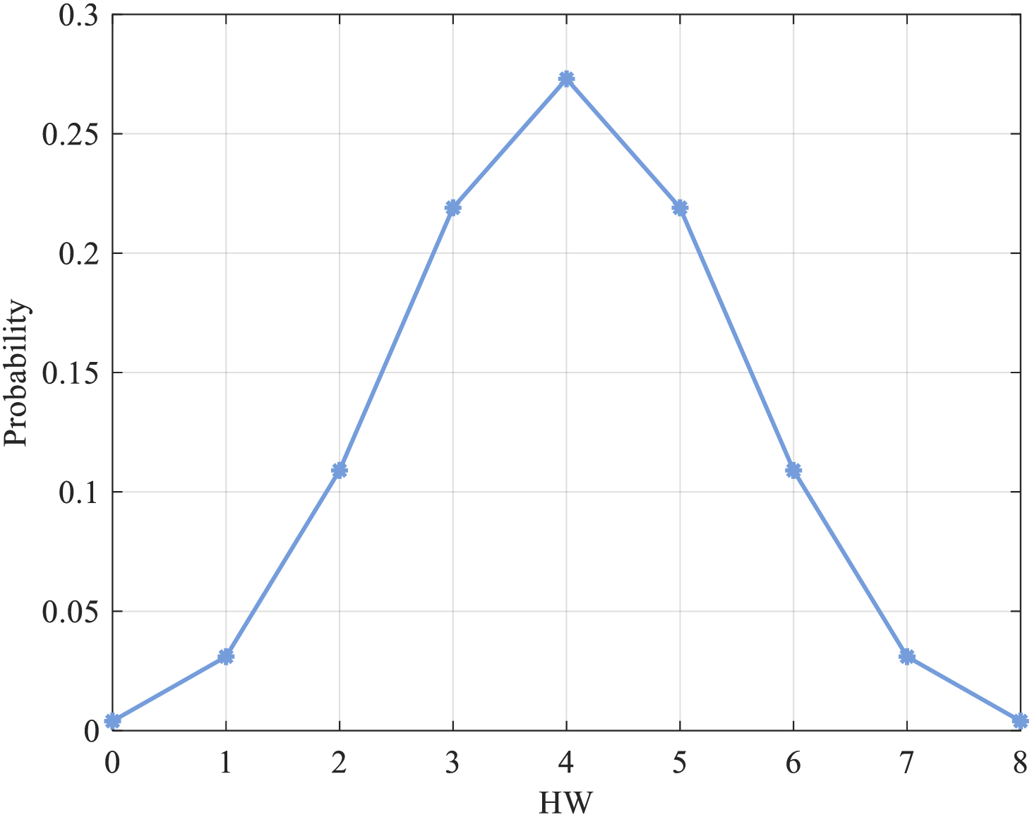
Figure 8: Probability distribution of HW for uniformly distributed single-byte data
Within the attack time window (880~900 ns), the distribution of fault probability of 256 plaintexts is shown in Fig. 9. It is observed that the distribution of the histogram is approximately composed of 9 normal distributions with different magnitudes. The mean of the first distribution is about 0.2911, the second distribution is about 0.3333, and the third distribution is about 0.3337, etc. This summary analyzes all the attack results within the determination window. It draws the following conclusion: when the data of the same HW is processed, the fault probability distribution is roughly the same. For the data of different HW, the means of each distribution are different, but the standard deviation is the same, and there are approximately nine normal distributions with other means.
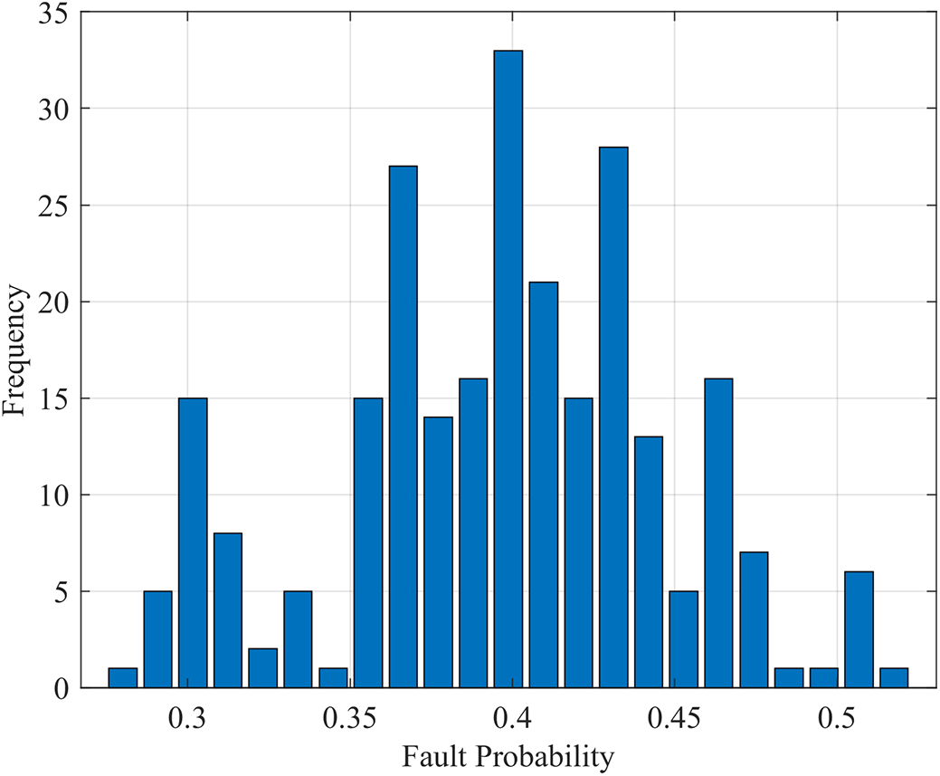
Figure 9: Frequency distribution of fault probability for different HW
The probability distribution of the same and different HW data will be analyzed below:
(1) Fault Probability Distribution for Data of the Same HW
Taking the attack results of two sets of the same HW data (HW 1 and 2) as an example, the fault probability of each time slice is shown in Table 4, respectively.
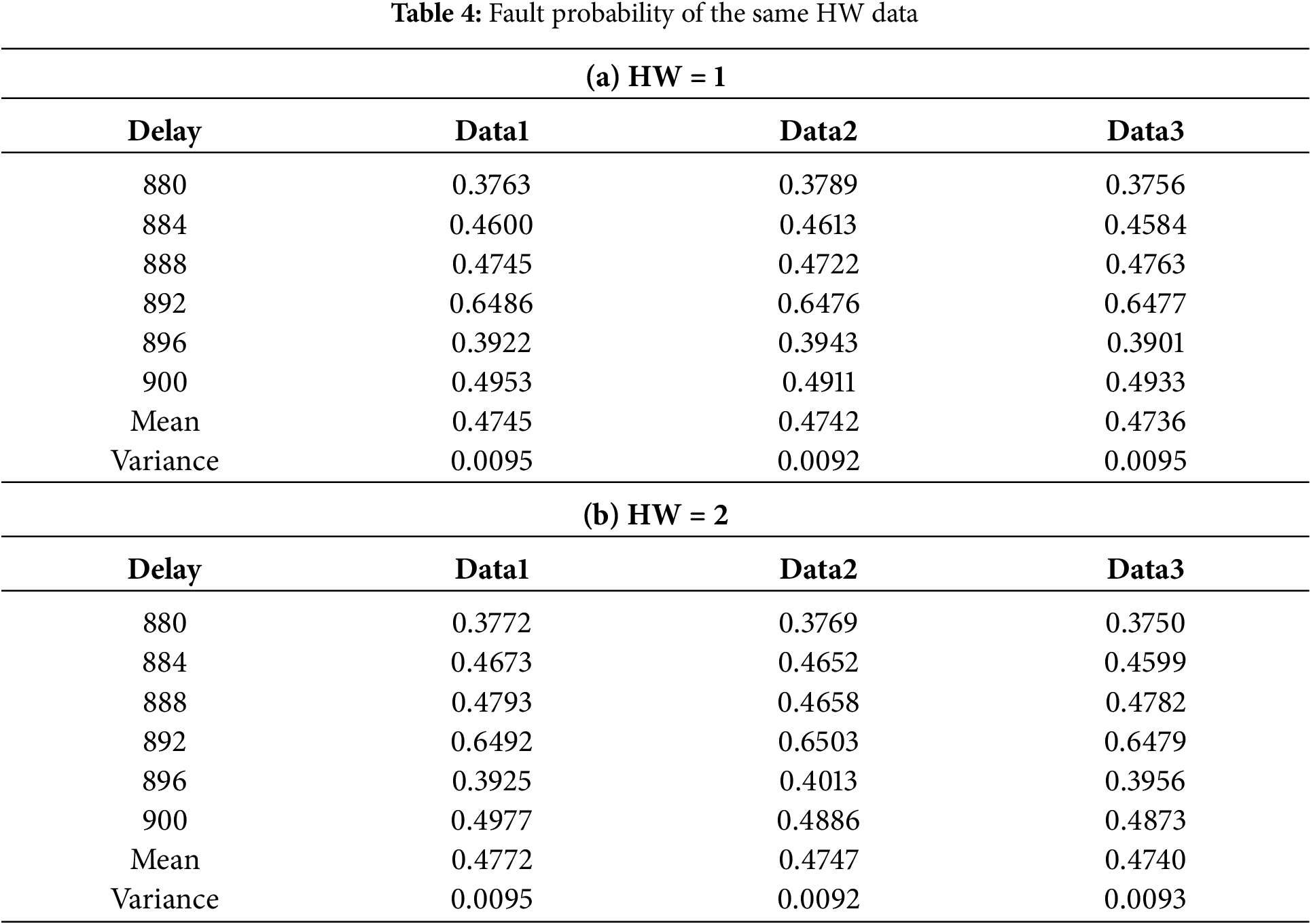
At the time of fault attack, the data with the same HW has very little difference in fault probability in each time slice. This means that the same HW data has the same fault mode. In Eq. (2), based on fixed P0 and P1, the fault probability PHWi is a constant for the same HW data. It is observed that the experimental results are consistent with this conclusion, and the above conclusion has been verified.
(2) Fault Probability Distribution for Data of Different HW
To remove electronic noise from the fault probability trace, we reduce the variance of FPel.noise by calculating the mean of multiple pieces of the same HW data. The diagram in Fig. 10 displays the probability distribution of faults in various HW. Each hardware data point has its distinct fault mode.
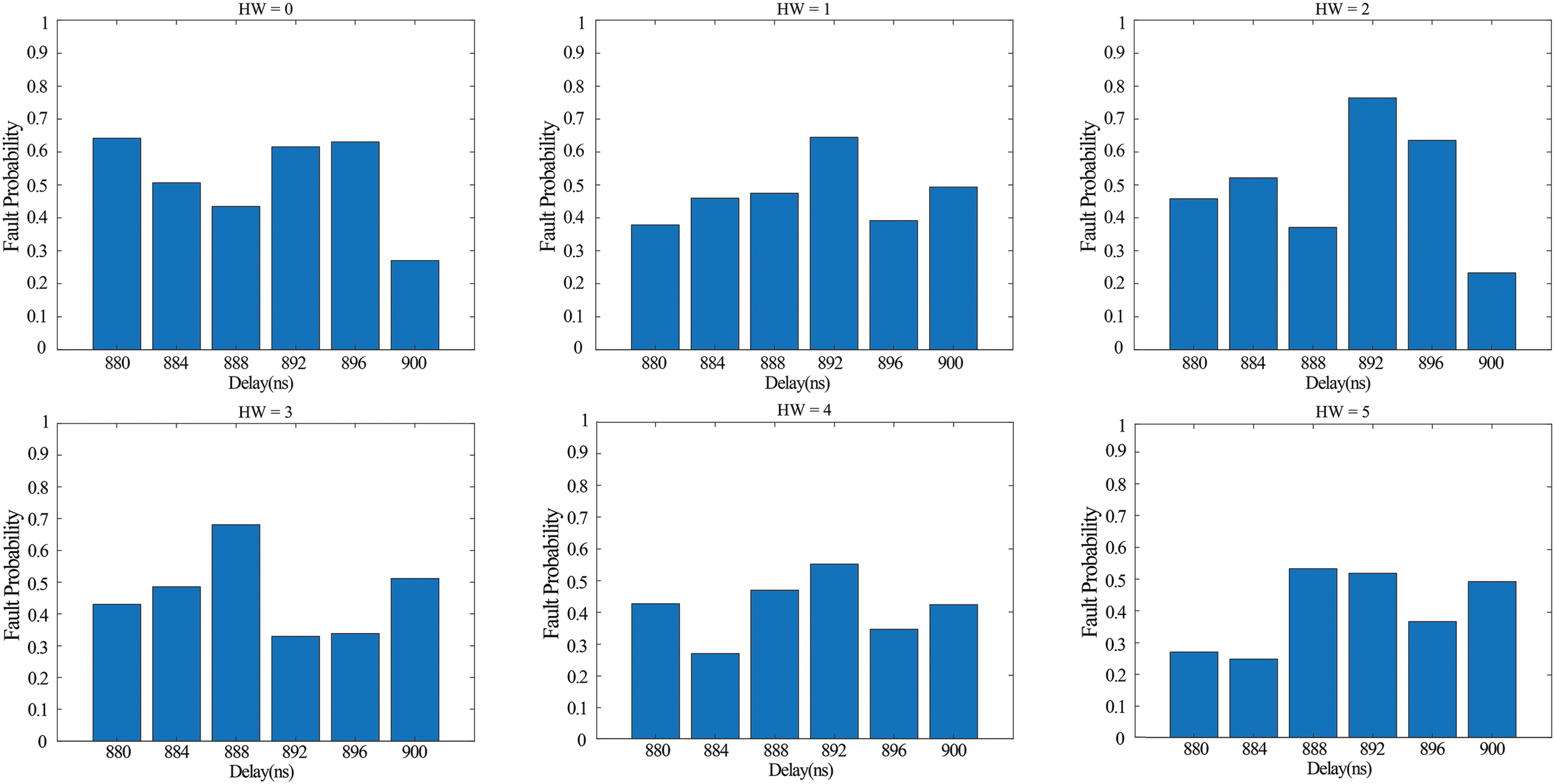
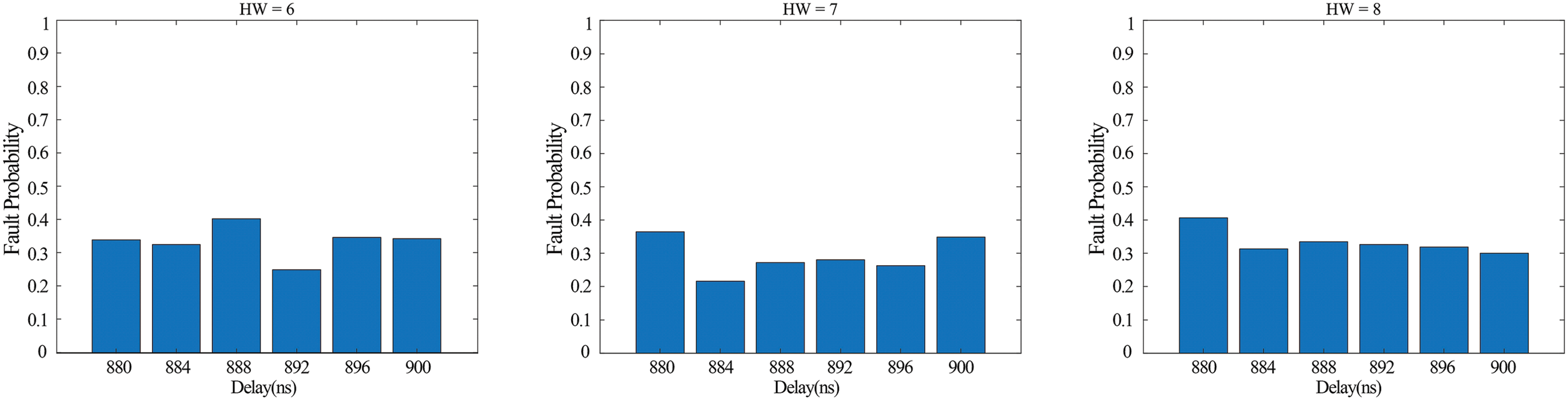
Figure 10: Fault probability distribution of data with different HW
The average of the fault probability for each HW data is presented in Fig. 11. The mean fault probability in the HW attack outcomes from 0 to 8 generally shows a decreasing trend, which aligns with the computational result of Eq. (2).
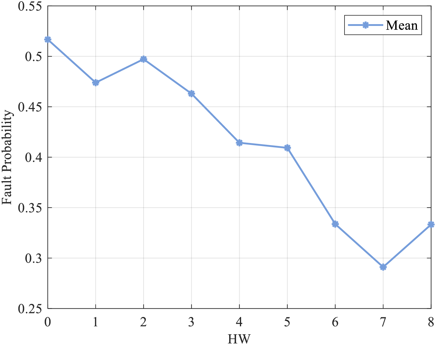
Figure 11: The mean of the fault probability of each HW data
The sliding window filtering method deals with the fault probability in each time slice. When the sliding window is 1 to 6, the correlation coefficient between fault probability and HW is shown in Fig. 12. When the delay window size is 6, the fault probability of the sixth time slice has the strongest correlation with the HW, up to −0.9455, showing a strong negative correlation. Reviewing Eq. (2), the fault probability of the output data is negatively correlated with its HW, and the theoretical and practical results are consistent.
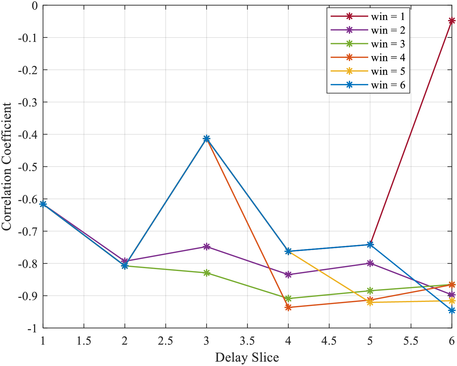
Figure 12: Correlation coefficient under sliding filtering
Since the fault probability of the sixth time slice with a delay window size of 6 has the strongest correlation with HW, the data is selected as the measured results for the following analysis. When PHW0 = 0.5167 and PHW8 = 0.3333 are substituted, P0 is 0.0534, and P1 is 0.0360. Substitute Eq. (2), and calculate the PHWi (i = 1, 2, …, 7), as shown in Table 5.
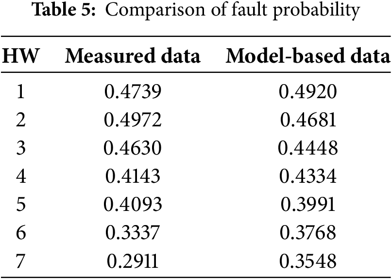
Fig. 13 illustrates that the correlation coefficient between the experimentally measured fault probabilities for each HW and those computed using Eq. (2) stands at 0.9403.

Figure 13: Comparison of fault probability based on actual measurement and model calculation
If the attack window and the selection of fault injection parameters are further optimized, the model fitting effect may be further improved. From the physical level, each memory cell (transistor and capacitor) in the general storage medium stores the data of 1 bit. The cell contains the electronic representation value “1” and empties the representation value “0”. After a capacitor is filled with electrons, it only takes a few milliseconds to leak out, so keeping the value of “1” requires the CPU to constantly charge the capacitor. Therefore, the energy consumption of 0→1 conversion is higher than that of 1→0 conversion in side-channel attacks. The energy consumption caused by data with higher HW is higher than that caused by data with lower HW [19].
In physical implementations, binary data “0” and “1” are represented by the charge states of transistor-capacitor units. Taking a CMOS inverter as an example, “1” corresponds to the capacitor charged to the logic high level, while “0” corresponds to the capacitor discharged to the logic low level. When a voltage glitch is injected, the charge stability of the capacitor directly affects the bit flip probability:
0→1 flip (charging state): Transistors must conduct to inject charge, and the capacitor is in a high-charge state. Voltage glitches are prone to cause overcharging or charge leakage.
1→0 flip (discharging state): Only transistor conduction is required to release charge, and the capacitor has less charge, resulting in higher tolerance to glitch interference.
For 8-bit data, the HW represents the number of “1” s. When the HW is higher, more capacitors are in the charged state, and the total charge is larger. Due to the capacitive coupling effect, collective charge fluctuations caused by voltage glitches are more likely to be suppressed, decreasing fault probability as the HW increases. This is consistent with the experimental results in Fig. 11, where the mean fault probability decreases as the HW increases from 0 to 8.
Therefore, the fault probability of 0→1 conversion is higher than that of 1→0 conversion. The fault probability of data with higher HW is lower than that of data with lower HW, similar to the data dependence of side channel attacks.
5 Design and Implementation of FPMIA
Existing mutual information analysis methods are all based on analog side-channel traces, such as power consumption or electromagnetic radiation. In contrast, FPMIA pioneers the application of MI to fault probability curves, constructing leakage models through frequency statistics of device response classifications. This innovation eliminates the need for analog signal acquisition equipment, requiring only the recording of digital device responses, thereby significantly expanding the applicability of fault attacks.
The specific process of FPMIA is shown in Fig. 14.
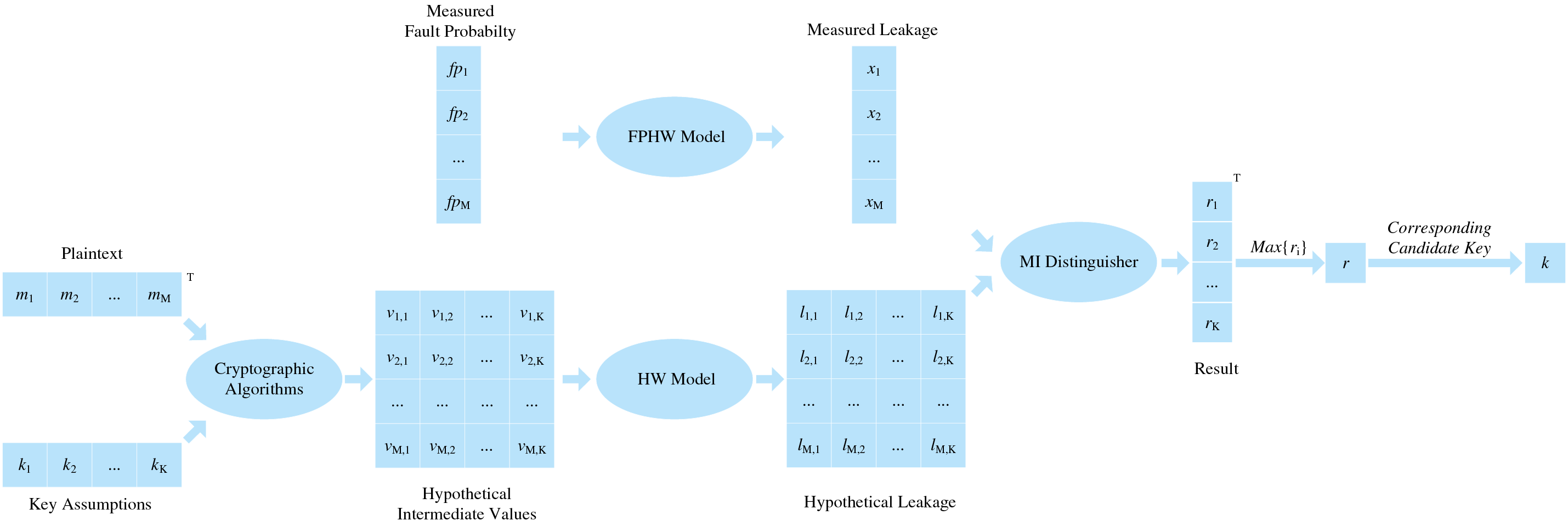
Figure 14: Attack flow of FPMIA
The steps of FPMIA are as follows:
• Step 1: Select an intermediate value of the executed algorithm. We chose the output of the first S-box in the initial round of AES-128 encryption.
• Step 2: Estimate the probability distribution of measured leakage. Many voltage glitches are injected into encrypting M plaintexts m = {m1, m2, …, mM}, and M fault probability traces are established. According to the FPHW model, the time delay corresponding to the leakage peak point is obtained, and the measured fault probability fp = {fp1, fp2, …, fpM} is obtained. Combined with the FPHW model, we use the Manhattan Distance method to map the measured fault probability to HWi (i = 0, 1, …, 8), obtain the measured leakage x = {x1, x2, …, xM} and estimate its probability density function.
• Step 3: Estimate the probability distribution of simulated leakage. For M plaintexts m = {m1, m2, …, mM} and K key assumptions k = {k1, k2, …, kK}, we calculate the hypothetical intermediate value.
We adopt the HW model and map the hypothetical intermediate value v to the simulated leakage.
• Step 4: Calculate the MI between the measured and simulated leakage to obtain r = {r1, r2, …, rK}. The guessed key (kg) corresponding to the maximum value is the correct key.
Estimating the probability distribution requires generating a PDF of the joint distribution, with kernel density estimation [20], data clustering [21], histogram method [22], vector quantization [23], and other methods. Among them, the histogram method estimates the probability density by grouping the data into bins; each bin covers a specific range and has an equal width. We use the histogram method to estimate the probability density, divide the leakage samples into 9 bins, and count the number of leakage samples falling into each bin. Next, we estimate the PDF of the simulated and measured leakage and analyze their relationship.
(1) Probability Distribution of Simulated Leakage
Randomly select 1000 plaintexts. Next, we take the 1st byte of four randomly selected key assumptions (kg = 0, 6, 198, 234) as an example, use random plaintext fragments and key fragments to calculate the intermediate value, and use the HW model for the leakage sample. The distribution was estimated. As shown in Fig. 15, the distribution of simulated leakage samples under different key assumptions is almost the same, and they all roughly obey the Gaussian distribution. Therefore, when the sample size is large enough, p(l) does not depend on the key assumption.

Figure 15: Distribution of simulated leakage under different key assumptions (a) kg = 0, (b) kg = 6, (c) kg = 198, (d) kg = 234
(2) Probability Distribution of Measured Leakage
We still use 1000 plaintexts above, choose the key k = 234, and attack the encryption process to obtain 1000 fault probability traces. Combined with the time delay corresponding to the S-box leakage peak interval, the fault probability corresponding to the time delay interval is mapped to HW by using the Euclidean Distance method according to the FPHW model.
Below, we illustrate the mapping process of measured fault probabilities with an example. We randomly select a fault probability trace and use the Euclidean Distance method to match it. The result is shown in Fig. 16. The x-axis HW represents the plaintext Hamming weight to which the leakage measurement may correspond, and the y-axis indicates the Euclidean distance between the fault probability of this trace and the Hamming weight. Since the Euclidean Distance is the shortest when HW = 1, the measured fault probability is mapped to the measured leakage HW = 1. Fig. 17 shows the probability distribution of the measured leakage corresponding to 1000 plaintexts when the key k = 234.
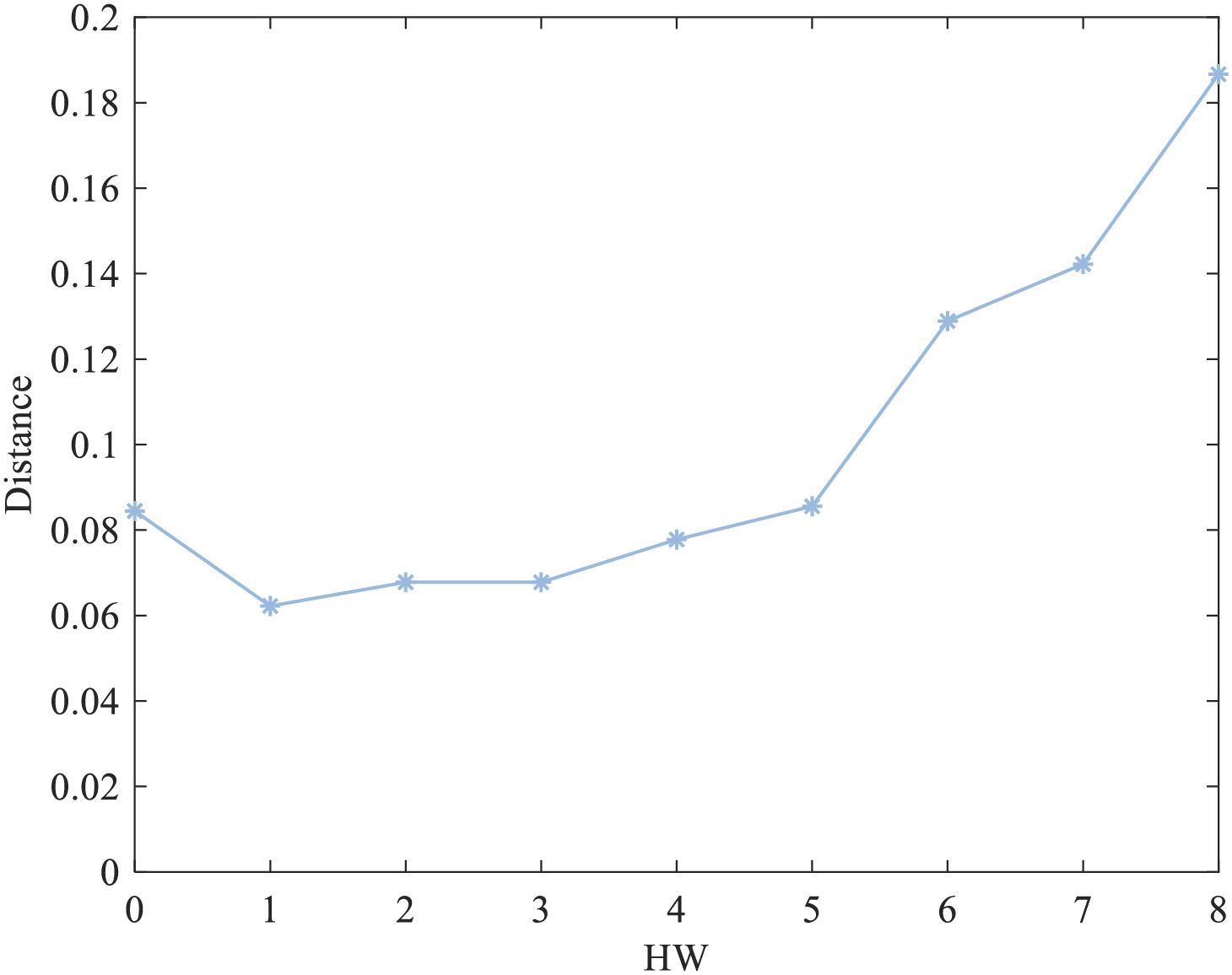
Figure 16: Mapping of measured fault probability to measured leakage

Figure 17: Distribution of measured values of fault probability
(3) Relationship between the Measured and Simulated Leakage
We choose the simulated leakage when the assumption key is 0, 6, 198, and 234, and study the relationship between it and the distribution of the measured leakage. We use Q-Q plots to represent the relationship between the simulated and measured leakage, as shown in Fig. 18. Fig. 18 depicts a Q-Q plot, which is a type of scatter plot. The x-axis represents the quantiles of one sample, while the y-axis corresponds to the quantiles of another sample. The scatter plot formed by the x- and y-axes represents the quantiles associated with the same cumulative probability. To identify whether the sample data follows a normal distribution using a Q-Q plot, one needs to observe whether the plot points are aligned along a straight line, with the slope of this line representing the standard deviation and the intercept being the mean. The blue line in Fig. 18 represents this straight line, where the x-axis indicates the quantiles of the simulated leakage samples, and the y-axis denotes the quantiles of the measured leakage samples. As shown in Fig. 18, when the kg is 234, the simulated and measured leakage distribution is the closest.

Figure 18: Relationship between simulated and measured leakage (a) kg = 0, (b) kg = 6, (c) kg = 198, (d) kg = 234
We use Eq. (7) to calculate the MI between the simulated and measured leakage under each key assumption, as shown in Fig. 19. When the kg is 234, the value of the MI is the largest. The key we used in the process is 234, and the result of the key recovery is successful. Thus, the MI metric successfully evaluates the actual leakage of the target device.

Figure 19: MI values corresponding to different key assumptions
The method of recovering the other bytes of the key is the same as described in this paper, and the ith byte of the key can be recovered by attacking the ith S-boxes encrypted in the 1st round of the AES-128 algorithm.
To verify the accuracy of FPMIA, we randomly generated plaintexts, the steps of which are shown in Algorithm 1.
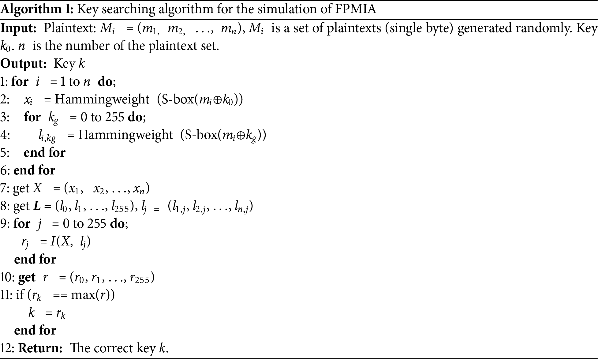
Numerous fault injection attacks are executed using random plaintexts to establish fault probability traces. As depicted in Fig. 20, the graph illustrates the correlation between the key recovery success rate and the quantity of fault probability traces.

Figure 20: MI values corresponding to different key assumptions
In Fig. 20, the trace number on the x-axis represents the quantity of fault probability traces used in the simulated attack. At the same time, the success rate on the y-axis indicates the probability of successfully recovering the key in the case of repeating a large number of experiments. When the count of fault probability traces exceeds 25, the attacker achieves a 100% likelihood of recovering the correct key.
In the MCU-based experiment, FPMIA is employed to conduct the attack, and the correlation between the key recovery success rate and the number of fault probability traces is presented in Fig. 21. When the quantity of fault probability traces surpasses 28, the attacker gains a 100% probability of recovering the correct key.
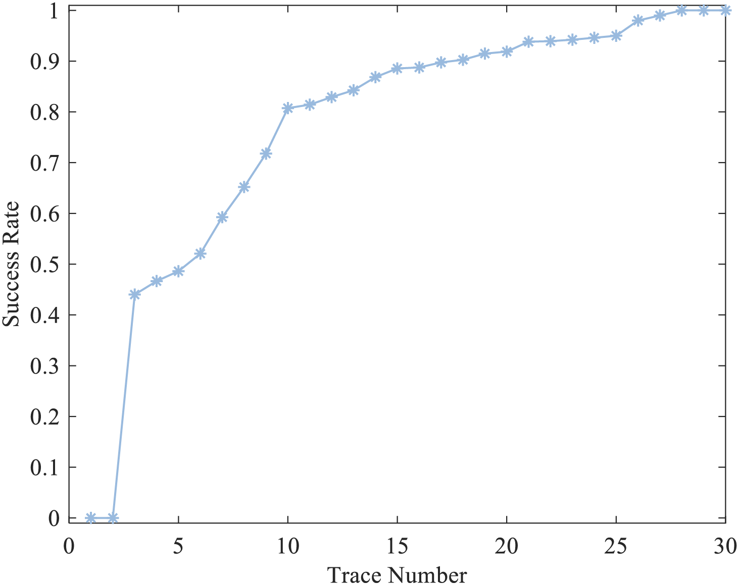
Figure 21: Result of the actual attack
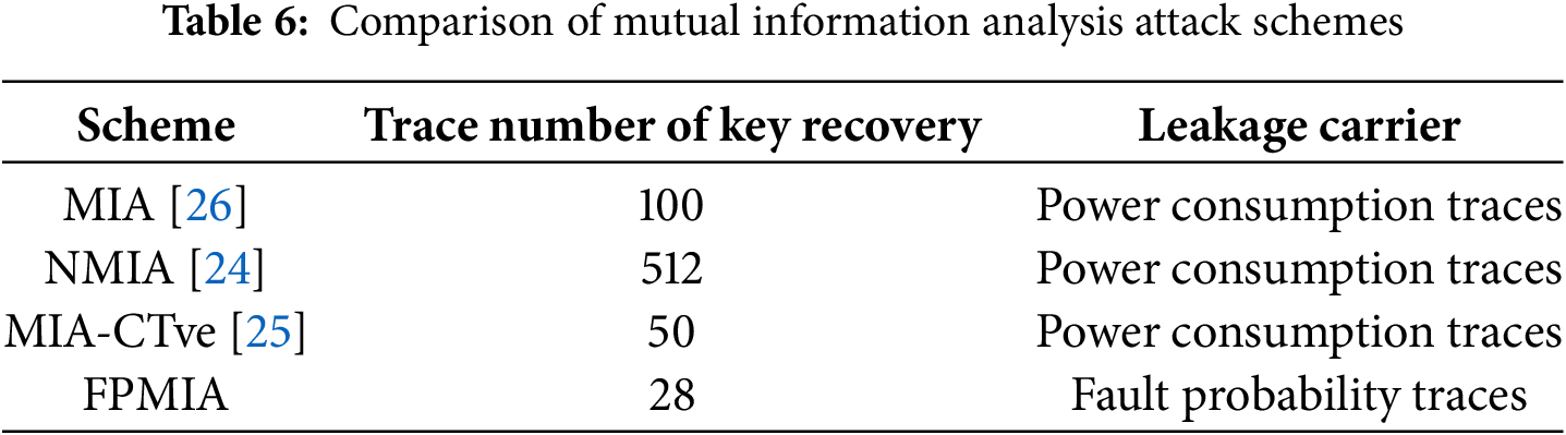
In recent years, a series of mutual information analysis attacks and their enhanced approaches have been successively put forward, such as NMIA [24] and MIA-CTve [25]. Next, compare the above mutual information analysis attack methods with FPMIA, as shown in Table 6, the FPMIA method increases the attack efficiency by at least 44%.
FPMIA achieves a 44% data reduction primarily due to three efficiency mechanisms:
(1) Noise suppression via statistical averaging. Each fault probability trace is generated by statistically classifying responses from numerous fault injections, suppressing random electronic noise via the law of large numbers.
(2) Strong physical correlation between HW and fault probability. Experiments measure a correlation coefficient of −0.9455 between fault probability and HW, with highly concentrated fault probability distributions for the same HW data forming 9 distinguishable normal distributions. This strong correlation allows the model to cover all HW scenarios with only 28 traces, whereas traditional methods require more data due to a weak power-HW correlation.
(3) Noise resistance of mutual information analysis. FPMIA uses MI to quantify “fault probability-HW” dependency, with MI invariant to independent noise (Eq. (7)). Even with residual noise, MI accurately captures true leakage if noise is independent of the key. Traditional MIA, based on correlation analysis, suffers from blurred peaks due to noise and requires more data for denoising.
The following describes the baseline methods, dataset details, and testing conditions to support the reproducibility of the experiments:
(1) baseline method comparison
To validate the efficacy of FPMIA, this study conducts a comparison with the subsequent mutual information analysis techniques:
MIA [26]: Based on the Hamming weight model, it uses the mutual information between measured power traces and simulated leakage to recover keys.
NMIA [24]: Employs a variational lower bound to estimate mutual information.
MIA-CTve [25]: Utilizes a mutual information-based distinguisher with a leakage model of cache access pattern vectors.
All comparative methods use the same plaintext set and fault injection parameters, executed on the STM32F405 platform.
(2) dataset composition
Plaintext Space: 256 8-bit plaintexts, with the first byte covering HW = 0 to HW = 8, and the remaining bytes fixed as 0x00 to isolate single-byte effects.
Number of Attacks: 1000 fault injections per plaintext.
Test Subset: Randomly sampled from the total number of traces.
(3) Experimental Environment and Parameters
Hardware Platform:
– Target device: STM32F405RGT6 microcontroller (DMCU-F405 encryption module).
– Fault injection equipment: Glitch generation module (voltage range: −6 V to 0 V, pulse width: 100–3000 ns).
Synchronous Triggering: Through a “large trigger-small trigger” dual-signal mechanism to ensure that glitch injection is synchronized with the AES first-round S-box operation.
Software Configuration: Encryption algorithm: AES-128 standard implementation using hardware-accelerated instructions.
Data acquisition: Record device responses.
The FPHW model is fundamentally different from existing HW-based leakage models, and its innovations are reflected in the following three aspects:
(1) Breakthrough in modelling logic: Existing models such as MIA rely on directly mapping “physical trace—HW”, requiring known plaintext/ciphertext and algorithm details. FPHW, however, establishes the correlation of “fault probability—HW” through device response classification probability statistics without needing specific data. In experiments, key recovery was achieved only through the response statistics of 256 groups of plaintexts with different HW, verifying the black-box attack capability independent of plaintext.
(2) Universality and implementation independence: FPHW proposes a decomposition framework of “operation dependence + data dependence”, where data dependence is determined solely by HW, and operation dependence is dynamically captured through response distribution. This makes the model independent of specific algorithms and hardware architectures, requiring only that device responses be classified into “normal/damaged” states.
(3) Data efficiency and noise robustness: The FPMIA method only requires 28 fault probability traces to recover the key with 100% success, reducing data requirements by 44% compared to traditional MIA. This benefits from the natural noise suppression of fault probability statistics—digital response classification is less susceptible to noise than analogue side-channel traces.
The FPHW model differs from previous general fault models, such as Fault Sensitivity Analysis (FSA) or Statistical Ineffective Fault Analysis (SIFA) in the following ways:
(1) “Zero-knowledge” data processing: Models like FSA/SIFA rely on plaintext-ciphertext pairs or intermediate values. For example, FSA requires calculating faulty ciphertext thresholds, and SIFA needs to judge whether intermediate values change. In contrast, FPHW only performs frequency statistics through 4 types of device response state classifications. When attacking 256 groups of plaintexts in experiments, it does not need to know the specific plaintext content. However, it only records the probability of “damaged” responses, enabling the establishment of a fault probability model and achieving true “data-independent” statistics.
(2) Physical-level breakthrough in modelling dimensions: Traditional models belong to “algorithm-level fault analysis” (e.g., FSA analyzes fault propagation paths in algorithms). At the same time, FPHW proposes a physical-level decomposition framework of “operation dependence + data dependence”. The data-dependent part is only related to data HW, and its negative correlation is derived from CMOS circuit charging/discharging mechanisms, completely decoupled from algorithm logic; the operation-dependent part is dynamically captured through response distribution, without knowing the specific operation type.
(3) Verification of black-box attack universality: FSA/SIFA assumes that attackers know algorithm implementations (white-box/grey-box). At the same time, FPHW only requires controlling fault injection parameters and observing response classifications (black-box). We recovered the key with 100% success in experiments using 28 fault probability traces without knowing the specific AES implementation. In contrast, FSA failed to attack without plaintext, verifying the universality of FPHW in black-box scenarios.
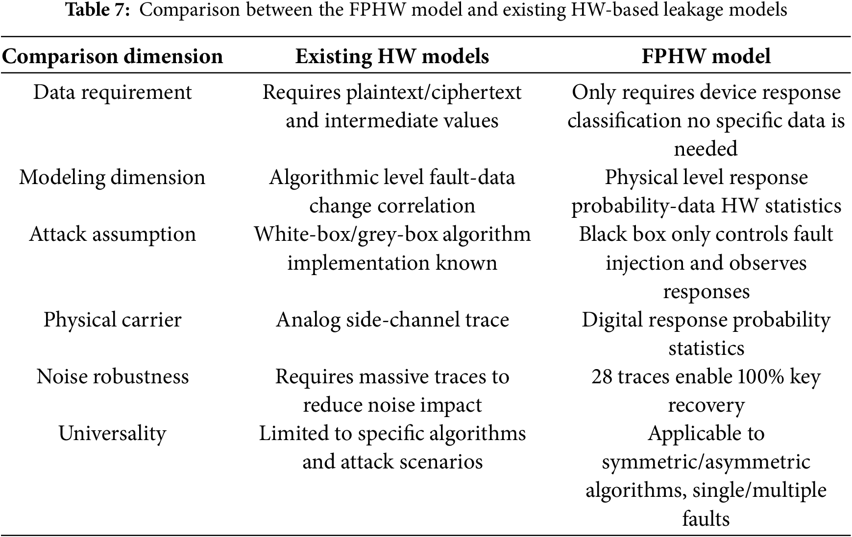
The comparison between the FPHW model and existing HW-based leakage models is shown in Table 7.
The core innovation of FPMIA lies in shifting MI analysis from “analogue signal correlation” to “digital probability statistics”. Since fault probability traces are statistical results of multiple injections, their noise robustness stems from statistical averaging to suppress random noise and MI’s invariance to independent noise (Eq. (7)). This makes FPMIA more practical in strong electromagnetic interference scenarios where traditional MI methods fail due to analog trace vulnerability.
This paper proposes the FPHW model and the FPMIA method. The FPHW model does not need to know the algorithm’s implementation details or detailed data, such as plaintext and intermediate values; it only needs to observe the target equipment’s response and count the probability of fault response.
The core of the FPHW model lies in decomposing fault probability into operation-dependent and data-dependent components, where the data-dependent component is directly related to the Hamming weight of the data. This modeling approach exhibits the following universality:
(1) Algorithm independence: The underlying layer of any cryptographic algorithm (symmetric/asymmetric) is based on binary bit operations. As a physical measure of data activity, HW directly reflects the charge state of storage units (such as the charging/discharging mode of CMOS transistors).
(2) Hardware independence: The model does not rely on specific processes (e.g., CMOS, FinFET) or architectures (MCU, FPGA), and only requires that device responses can be classified as “corruption/others” states.
Because the derivation process and conclusions apply to all types of fault attacks, the model is universal and can solve the problem of the lack of a unified model to describe fault attacks. The model is suitable for template fault attacks, differential fault attacks, fault correlation attacks, and so on.
Through a large number of fault injection experiments and result analysis, the following conclusions can be drawn:
(1) The fault probability distribution of the same HW data is the same. However, the fault probability distribution of different HW data is quite different due to their different fault modes, which is consistent with the theoretical analysis conclusion of this model.
(2) The FPHW model can accurately describe the information leakage of the fault attack. The correlation coefficient between the theoretically calculated fault probability and the measured one is as high as 0.9403, and the fault probability and the data’s HW are dependent.
The essence of the fault is that a single bit has been flipped accidentally, and the essence of the bit flip is the charging and discharging behavior of the central processing unit (CPU) to the capacitor. In the side-channel attack, the effect of random bit flips is reflected in the difference in energy consumption. As for fault injection attacks, it is reflected in the difference in fault probability. They show that side-channel and fault injection attacks obtain sensitive information from different dimensions, and their essence is consistent. This conclusion lays the foundation for establishing a unified physical security leakage model.
Taking the implementation of the AES-128 algorithm based on the MCU as an example, the attacker successfully achieved key recovery using 28 fault probability traces. This method mainly has the following advantages:
(1) Less affected by noise. We chose the FPHW model, which does not need to collect ciphertext and only focuses on the response of the target device after the attack, which is hardly affected by noise. The noise resistance of FPMIA stems from the robustness of its statistical modeling and the noise tolerance of mutual information. Fault probability traces are statistical results of multiple fault injections, which suppress random noise based on the law of large numbers. Meanwhile, because mutual information is invariant to independent noise, noise does not affect the identification of mutual information peaks between keys and leakage. Even if Gaussian noise exists in fault probability traces, as long as the noise is independent of the key, MI can still effectively capture the correlation between actual leakage and the key.
(2) Strong scalability. This method does not depend on specific assumptions and detailed algorithm steps and can be easily extended to more dimensions, such as attacks on mask-protected cryptographic devices. The FPHW model can be extended to multi-round attacks on block ciphers, key stream analysis of stream ciphers, and even fault analysis of exponential operations in public-key algorithms. The core assumption of the FPHW model is that fault probability depends on the data Hamming weight (HW) and operation types. For block cipher algorithms, the HW of intermediate values reflects the activity level of data bits, and the negative correlation between fault probability and HW can be derived through circuit-level charging/discharging mechanisms. For public-key cryptographic algorithms such as RSA, modular exponentiation consists of binary bit operations—the higher the exponent or modulus’s HW, the greater the corresponding register’s total charge, and the lower the flip probability after fault injection. Therefore, this assumption applies to all cryptographic algorithms based on binary representation. Meanwhile, the model does not rely on specific hardware architectures and only requires device responses to be classifiable as “corruption/others” states, ensuring cross-platform applicability.
Finally, several prospects for future work are put forward:
• We will consider attacks based on multiple hardware platforms, targeting different cryptographic algorithms, and encrypted targets protected by masking.
• In experiments, we observe that measuring physical leakage is much easier than calculating key recovery efficiency. Since the amount of MI can also be used to evaluate the leakage of the target device, that is, the physical security, if we can find out the relationship between the amount of MI and the attack success rate, the efficiency of security assessment can be significantly improved.
• We will also conduct verification experiments on noise robustness from controlled noise injection and hardware noise comparison. Gaussian noise with known SNR will be added to the fault probability curves to test the relationship between key recovery success rate and SNR; a programmable noise source will be introduced on the FPGA platform to compare the performance of FPMIA and other methods under the same noise level.
• We will conduct algorithmic abstract modeling to derive the theoretical relationship between HW and fault probability in different algorithms based on formal descriptions of cryptographic algorithms, establishing a unified cross-algorithm analysis framework. Meanwhile, we will develop adaptive filtering algorithms to estimate and eliminate environmental noise from fault probability curves in real time, enhancing reliability in complex scenarios.
• Finally, we contemplate incorporating novel methodologies such as machine learning in our future endeavors to analyze fault response distribution maps and select fault injection parameters, thereby enhancing the efficiency of our analysis.
Acknowledgement: Not applicable.
Funding Statement: The authors received no specific funding for this study.
Author Contributions: The authors confirm contribution to the paper as follows: Conceptualization, Tong Wu; methodology, Tong Wu; software, Tong Wu; validation, Tong Wu, Dawei Zhou; formal analysis, Tong Wu; investigation, Tong Wu; resources, Dawei Zhou; data curation, Tong Wu; writing—original draft preparation, Tong Wu; writing—review and editing, Tong Wu, Dawei Zhou; visualization, Tong Wu; supervision, Dawei Zhou; project administration, Dawei Zhou. All authors reviewed the results and approved the final version of the manuscript.
Availability of Data and Materials: The data that support the findings of this study are available from the Corresponding Author, Tong Wu, upon reasonable request.
Ethics Approval: Not applicable.
Conflicts of Interest: The authors declare no conflicts of interest to report regarding the present study.
Abbreviations
| FPHW | Fault probability model based on Hamming Weight |
| FPMIA | A fault injection attack method based on the FPHW model from the perspective of mutual information |
| MCU | Microcontroller Unit |
| MIA | Mutual Information Analysis |
| FCA | Fault Correlation Analysis |
| CPA | Correlation Power Analysis |
References
1. Alshaer I, Burghoorn G, Colombier B, Deleuze C, Beroulle V, Maistri P. Cross-layer analysis of clock glitch fault injection while fetching variable-length instructions. J Cryptogr Eng. 2024;14(2):325–42. doi:10.1007/s13389-024-00352-6. [Google Scholar] [CrossRef]
2. Xu J, Zhang F, Jin W, Yang K, Wang Z, Jiang W, et al. A deep Investigation on stealthy DVFS fault injection attacks at DNN hardware accelerators. IEEE Trans Comput-Aided Des Integr Circuits Syst. 2025;44(1):39–51. doi:10.1109/TCAD.2024.3426364. [Google Scholar] [CrossRef]
3. Hayashi S, Sakamoto J, Matsumoto T. Design methodology of digital sensors for detecting laser fault injection attacks in FPGAs. J Cryptogr Eng. 2025;15(2):12. doi:10.1007/s13389-025-00378-4. [Google Scholar] [CrossRef]
4. Hyunju Kim, Im W, Jeong S, Hyunil Kim, Seo C, Kang C. Recovery for secret key in CTIDH-512 through fault injection attack. Comput Electr Eng. 2025;123(2):110057. doi:10.1016/j.compeleceng.2024.110057. [Google Scholar] [CrossRef]
5. Casado-Galán A, Potestad-Ordóñez FE, Acosta AJ, Tena-Sánchez E. Electromagnetic fault injection attack methodology against AES hardware implementation. In: Proceedings of the 2024 39th Conference on Design of Circuits and Integrated Systems (DCIS); 2024 Nov 13–15; Catania, Italy. Piscataway, NJ, USA: IEEE; 2024. Vol. 6225. p. 1–6. doi:10.1109/DCIS62603.2024.10769137. [Google Scholar] [CrossRef]
6. Esmaeilian M, Beitollahi H. Experimental evaluation of RISC-V micro-architecture against fault injection attack. Microprocess Microsyst. 2024;104(1):104991. doi:10.1016/j.micpro.2023.104991. [Google Scholar] [CrossRef]
7. Li Y, Sakiyama K, Gomisawa S, Fukunaga T, Takahashi J, Ohta K. Fault sensitivity analysis. In: Mangard S, Standaert FX, editors. Cryptographic hardware and embedded systems-CHES 2010. Lecture notes in computer science. Berlin/Heidelberg, Germany: Springer; 2010. p. 320–34. doi:10.1007/978-3-642-15031-9_22. [Google Scholar] [CrossRef]
8. Ghalaty NF, Yuce B, Taha M, Schaumont P. Differential fault intensity analysis. In: Proceedings of the: 2014 Workshop on Fault Diagnosis and Tolerance in Cryptography, FDTC 2014; 2014 Sep 23; Busan, Republic of Korea. p. 49–58. doi:10.1109/FDTC.2014.15. [Google Scholar] [CrossRef]
9. Dobraunig C, Eichlseder M, Korak T, Mangard S, Mendel F, Primas R. Sifa: exploiting ineffective fault inductions on symmetric cryptography. IACR Trans Cryptogr Hardw Embed Syst. 2018;2018(3):547–72. doi:10.13154/tches.v2018.i3.547-572. [Google Scholar] [CrossRef]
10. Saha S, Bag A, Roy DB, Patranabis S, Mukhopadhyay D. Fault template attacks on block ciphers exploiting fault propagation. In: Canteaut A, Ishai Y, editors. Advances in cryptology—eurocrypt 2020, PTI. Lecture notes in computer science. Cham, Switzerland: Springer International Publishing; 2020. Vol. 12105, p. 612–43. doi:10.1007/978-3-030-45721-1_22. [Google Scholar] [CrossRef]
11. Spruyt A, Milburn A, Chmielewski Ł. Fault injection as an oscilloscope: fault correlation analysis. IACR Trans Cryptogr Hardw Embed Syst. 2020;2020:192–216. doi:10.46586/tches.v2021.i1.192-216. [Google Scholar] [CrossRef]
12. Degré M, Derbez P, Lahaye L, Schrottenloher A. New models for the cryptanalysis of ASCON. Des Codes Cryptogr. 2025;93(6):2055–72. doi:10.1007/s10623-025-01572-5. [Google Scholar] [CrossRef]
13. Wu X, Li J, Zhang R, Zhang H. A novel two-stage model based SCA against secAES. J Electron Test. 2024;40(6):707–21. doi:10.1007/s10836-024-06149-z. [Google Scholar] [CrossRef]
14. Argiento R, Filippi-Mazzola E, Paci L. Model-based clustering of categorical data based on the hamming distance. J Am Stat Assoc. 2025;120(550):1178–88. doi:10.1080/01621459.2024.2402568. [Google Scholar] [CrossRef]
15. Jiao L, Li Y, Hao Y, Gong X. Differential fault attacks on privacy protocols friendly symmetric-key primitives: rain and hera. IET Inf Secur. 2024;2024(1):519. doi:10.1049/2024/7457517. [Google Scholar] [CrossRef]
16. Zhang X, Jiang Z, Ding Y, Ngai ECH, Yang SH. Anomaly detection using isomorphic analysis for false data injection attacks in industrial control systems. J Frankl Inst. 2024;361(13):107000. doi:10.1016/j.jfranklin.2024.107000. [Google Scholar] [CrossRef]
17. Guo Z, Zhao R, Huang Z, Jiang Y, Li H, Deng Y. Transient voltage information entropy difference unit protection based on fault condition attribute fusion. Entropy. 2025;27(1):61. doi:10.3390/e27010061. [Google Scholar] [PubMed] [CrossRef]
18. Nassar H, Krautter J, Bauer L, Gnad D, Tahoori M, Henkel J. Meta-scanner: detecting fault attacks via scanning FPGA designs metadata. IEEE Trans Comput-Aided Des Integr Circuits Syst. 2024;43(11):3443–54. doi:10.1109/TCAD.2024.3443769. [Google Scholar] [CrossRef]
19. Mangard S, Oswald E, Popp T. Power analysis attacks: revealing the secrets of smart cards. Heidelberg, Germany: Springer Science & Business Media; 2008. Vol. 31. [Google Scholar]
20. Moreo A, González P, del Coz JJ. Kernel density estimation for multiclass quantification. Mach Learn. 2025;114(4):92. doi:10.1007/s10994-024-06726-5. [Google Scholar] [CrossRef]
21. Wang Y, Qian J, Hassan M, Zhang X, Zhang T, Yang C, et al. Density peak clustering algorithms: a review on the decade 2014–2023. Expert Syst Appl. 2024;238(7):121860. doi:10.1016/j.eswa.2023.121860. [Google Scholar] [CrossRef]
22. Pérez-Mon O, Moreo A, Coz JJé del, González P. Quantification using permutation-invariant networks based on histograms. Neural Comput Appl. 2025;37(5):3505–20. doi:10.1007/s00521-024-10721-1. [Google Scholar] [CrossRef]
23. Wang J-Y, Du T, Chen L. Undersampling based on generalized learning vector quantization and natural nearest neighbors for imbalanced data. Int J Mach Learn Cybern. 2024;21(9):1263. doi:10.1007/s13042-024-02261-w. [Google Scholar] [CrossRef]
24. Zhang C, Lu X, Cao P, Gu D, Guo Z, Xu S. A nonprofiled side-channel analysis based on variational lower bound related to mutual information. Sci China Inf Sci. 2023;66(1):112302. doi:10.1007/s11432-021-3451-1. [Google Scholar] [CrossRef]
25. Guo P, Yan Y, Zhang F, Zhu C, Zhang L, Dai Z. Extending the classical side-channel analysis framework to access-driven cache attacks. Comput Secur. 2023;129:103255. doi:10.1016/j.cose.2023.103255. [Google Scholar] [CrossRef]
26. Gierlichs B, Batina L, Tuyls P, Preneel B. Mutual information analysis: a generic side-channel distinguisher. In: Proceedings of the International Workshop on Cryptographic Hardware and Embedded Systems; 2008 Aug 10–13; Washington, DC, USA. p. 426–42. [Google Scholar]
Cite This Article
 Copyright © 2025 The Author(s). Published by Tech Science Press.
This work is licensed under a Creative Commons Attribution 4.0 International License , which permits unrestricted use, distribution, and reproduction in any medium, provided the original work is properly cited.
 Downloads
 Citation Tools