Identification of Visibility Level for Enhanced Road Safety under Different Visibility Conditions: A Hierarchical Clustering-Based Learning Model

1  Introduction

Visibility is a crucial meteorological factor for ensuring the safety of road and air traffic, particularly under adverse weather conditions. Poor visibility, often caused by dense fog, heavy rain, snow, or sandstorms, can severely affect a driver’s ability to see other vehicles, road lines, traffic signals, and signs, leading to an increased risk of accidents [1]. Among the mentioned factors, fog is a major concern that often occurs in different areas and greatly affects road safety. Numerous research studies have been accomplished for addressing this issue; however, they choose a particular region as a case study and are not generic [2]. Furthermore, the earlier methodologies primarily rely on conventional techniques that may be suitable for one specific scenario but may not be effective across different case studies with varying visibility conditions.

Recent technological advances in machine learning (ML) and deep learning (DL) have greatly improved different application areas such as surveillance, transportation systems, etc. Advanced ML, DL, and video-based visibility detection methods [3,4] offer a cost-effective alternative to one of the prominent traditional methods known as laser visibility meters [5], image processing, and AI-based techniques [6] to estimate the visibility level under different weather conditions. Some of these methods, like those that use dark channel prior (DCP) knowledge to estimate transmittance [7] for classification [8], have various limitations because they depend on static images and indirect calculations, which make them less accurate. Furthermore, methods leveraging continuous image evolution for fog prediction showed better performance; however, they still struggle with precise visibility estimation [9].

Keeping the significance of advanced ML and DL techniques in mind, this study proposes an ML-based approach for estimating visibility levels under different circumstances to ensure continuous traffic flow and help drivers avoid road accidents. The objective of this study is to give drivers real-time visibility updates using highway CCTV (Closed-Circuit Television) cameras, which are already installed along the roadside every 2 km for traffic monitoring. The CCTV cameras are used because they are widely used for surveillance and offer a cost-effective and practical solution for road monitoring and traffic surveillance. By analyzing the camera images, the system estimates how far drivers can see ahead and quickly shares this information with them. This helps drivers slow down or take safety measures in foggy and poor weather conditions, reducing accident risks. The approach is cost-effective since it uses existing cameras compared to deploying specialized and expensive visibility measurement devices. This method not only improves road safety but also supports the growing need for intelligent transportation systems capable of operating safely in low-visibility conditions. Furthermore, we focus on avoiding the use of threshold-based approaches because images captured under different conditions, such as different dates and weather scenarios, produce varying data patterns. This makes it difficult to apply a single threshold for visibility measurement. Instead, we extract data patterns from the CCTV images and estimate visibility distance using hierarchical clustering. This study uses CCTV images with eight different visibility levels to identify the visibility level and fog level under diverse weather conditions.

The main contributions of this study are listed as follows:

•   This study introduces a real-time visibility estimation model that leverages roadside CCTV cameras, focusing on ROIs in the captured frames to extract features that are crucial for distinguishing visibility levels under varying weather conditions.

•   The proposed approach consists of two main parts, i.e., feature extraction and hierarchical clustering. For feature extraction, we develop a method to extract specific features, namely the number of lines and contours, from ROI-based analysis of CCTV images. These features are very vital and effective indicators of visibility levels, with distinct patterns observed between high and low visibility scenarios. For visibility level estimation, we employ hierarchical clustering using DTW, a similarity metric, to classify visibility levels. The proposed approach allows for adaptive classification without relying on fixed thresholds, improving the robustness of the model under diverse environmental conditions.

•   Our proposed approach achieved over 97% accuracy, which proves its effectiveness and reliability as compared to traditional methods. Our approach provides great potential for enhancing road safety in adverse low-visibility weather conditions. Additionally, using the proposed system with current roadside CCTV cameras provides an effective way to monitor traffic in real-time and keep drivers informed about visibility conditions. This helps enhance road safety in diverse weather conditions.

The rest of the paper is organized as follows: Section 2 provides a detailed overview of the literature review. Section 3 illustrates the proposed methodology. Section 4 demonstrates the detailed experimental results and evaluation. Finally, Section 5 summarizes the main findings of this study and provides future research directions for further investigation of the topic.

2  Related Work

Meteorological visibility level estimation is very crucial for traffic safety, environmental monitoring, and urban surveillance. Visibility estimation for road safety under diverse weather conditions has been explored in different studies using numerous approaches. For instance, the authors in [10,11] used physical sensors, while reference [12] utilized a computer vision-based approach for visibility identification using CCTV videos. The use of CCTV cameras for visibility estimation has emerged as one of the most prevalent techniques [13]. In this section, we review the existing visibility estimation techniques, which are given in more detail in the following subsections.

2.1 Farthest Black Object-Based Approach

In this approach the visibility distance is calculated via different fixed black objects; the farthest visible black object represents the visibility distance. It uses different techniques like thresholding and image segmentation to identify different targets along the road. The targets include lane markers, road signs, and the intersection lines. The camera is geometrically calibrated to get the highest accuracy. According to [14], the visibility is defined by the International Commission on Illumination (CIE) as the distance at which a black object of a specific size is visible with less than 5% contrast. This approach takes advantage of using a single camera, but it requires that the road and the sky be visible in the image scenery. Kim [15] compared how far people can see with their eyes, human visual range (HVR), and how visibility can be measured using meteorological tools. They found that using images to measure visibility was more accurate, especially when the entire scene was captured. In a similar study, Yang et al. [16] developed a method to estimate visibility in real-time for adaptive speed limit systems in smart traffic systems. They used road images and analyzed them with techniques like DCP, weighted image entropy, and support vector machines (SVM) to get accurate visibility estimates.

2.2 Scene Contrast Calculation Methods

This method calculates visibility based on the contrast of the scene. By employing linear regression, the relationship between scene contrast and visibility is established. In this regard, Wang et al. [17] developed a technique to detect atmospheric visibility by comparing the brightness of images, focusing on the difference between the brightness of a specific target and the sky area in the background.

To further improve visibility estimation, different studies have adopted feature-based approaches, which analyze specific image features rather than the entire frame [18]. Common extracted features include edge density, texture information, and geometric structures. Edge-based methods, such as Canny edge detection and Hough transform for line detection, have been widely used to analyze scene clarity [19]. Several studies have shown that detecting and counting specific straight-line structures in images (e.g., road lane markings, building edges, and object boundaries) can serve as a reliable indicator of visibility levels [20]. Under clear conditions, images contain more distinct lines, whereas fog or haze reduces their detectability. This approach is particularly effective in structured environments such as urban roads, where the features degrade in a predictable manner under low visibility levels.

2.3 Global Image Descriptor-Based Approach

This approach estimates visibility by calculating global descriptors from the entire image. With the advancement of artificial intelligence (AI) in recent times, neural networks have become a key tool in computer vision, leading to a wide range of new applications. For instance, Chaabani et al. [21] used the Fourier transform to extract global image features and trained a three-layer neural network to identify different visibility levels. This approach effectively eliminates the need for edge detection or a referenced target distance. Palvanov and Cho [22] introduced a visibility estimation method using a deep hybrid convolutional neural network (DHCNN) combined with a two-step Laplacian of Gaussian (LoG) filter, which accurately estimates visibility distance. Chaabani et al. [23] presented a method that combines CNN and SVM classifiers, where the CNN extracts image features that are then classified by the SVM. This method shows promising results in obstacle avoidance systems. Likewise, Outay et al. [24] proposed a novel approach for estimating visibility range in foggy conditions using the standard AlexNet [25] architecture using the DCNN algorithm with raw image data for feature extraction and SVM for classification purposes. Yu et al. [26] also trained an ANN using meteorological data (temperature, humidity, air pressure, and wind speed) and image data (saturation, minimum grey value, and contrast) as input, with visibility as the output. The error between predicted and actual visibility with this method was 7.56%.

Traditional image-based approaches estimate visibility by analyzing contrast attenuation and colour degradation in images [27]. Contrast-based methods measure the loss of contrast in distant objects due to atmospheric haze [28], while DCP-based techniques estimate haze intensity by detecting pixels with low intensity in at least one colour channel [29,30]. However, these approaches are sensitive to illumination variations, camera angles, and scene complexity and are mostly threshold-based. Additionally, they focus on entire images rather than specific ROIs, making them less effective in structured environments like roads, where certain features (e.g., lane markings, edges, and objects) are more informative. Early studies mostly focus on dedicated meteorological instruments such as transmissometers [5,13], LIDAR [31], and ceilometers [32] to measure visibility by analyzing light scattering and absorption. These methods provide better performance; however, they have high deployment costs, limited spatial coverage, and sensitivity to local environmental factors.

2.4 Machine Learning and Clustering-Based Approaches

ML techniques, especially unsupervised approaches [33], have been employed to classify visibility conditions based on extracted features. Hierarchical clustering is particularly suitable for this task as it groups similar patterns into nested clusters, allowing for adaptive classification of varying visibility levels [34]. Unlike threshold-based methods, clustering techniques automatically determine relationships between feature distributions without requiring predefined visibility categories.

Based on existing methods, our method estimates visibility by analyzing structural features (lines, contours) in specific regions of CCTV video frames. Using hierarchical clustering for unsupervised classification and DTW as a distance metric for feature alignment, this region-based approach improves upon full-frame analysis methods. The technique offers robust visibility estimation while maintaining computational efficiency for real-time transportation monitoring applications, with advantages in adaptability and handling of temporal variations.

3  Proposed Methodology

The proposed system shown in Fig. 1 has two main steps: (1) extracting data patterns and (2) learning through clustering. First, frames from CCTV footage were extracted by focusing on specific road areas (ROIs). These ROIs help in detecting the visibility because the extracted features (lines and contours) have distinct values in different weather conditions. Next, using hierarchical clustering, we grouped similar images based on visibility using DTW as a similarity measure. Each cluster represents a visibility level, enabling accurate classification. The following subsections further explain the methodology of the proposed approach.

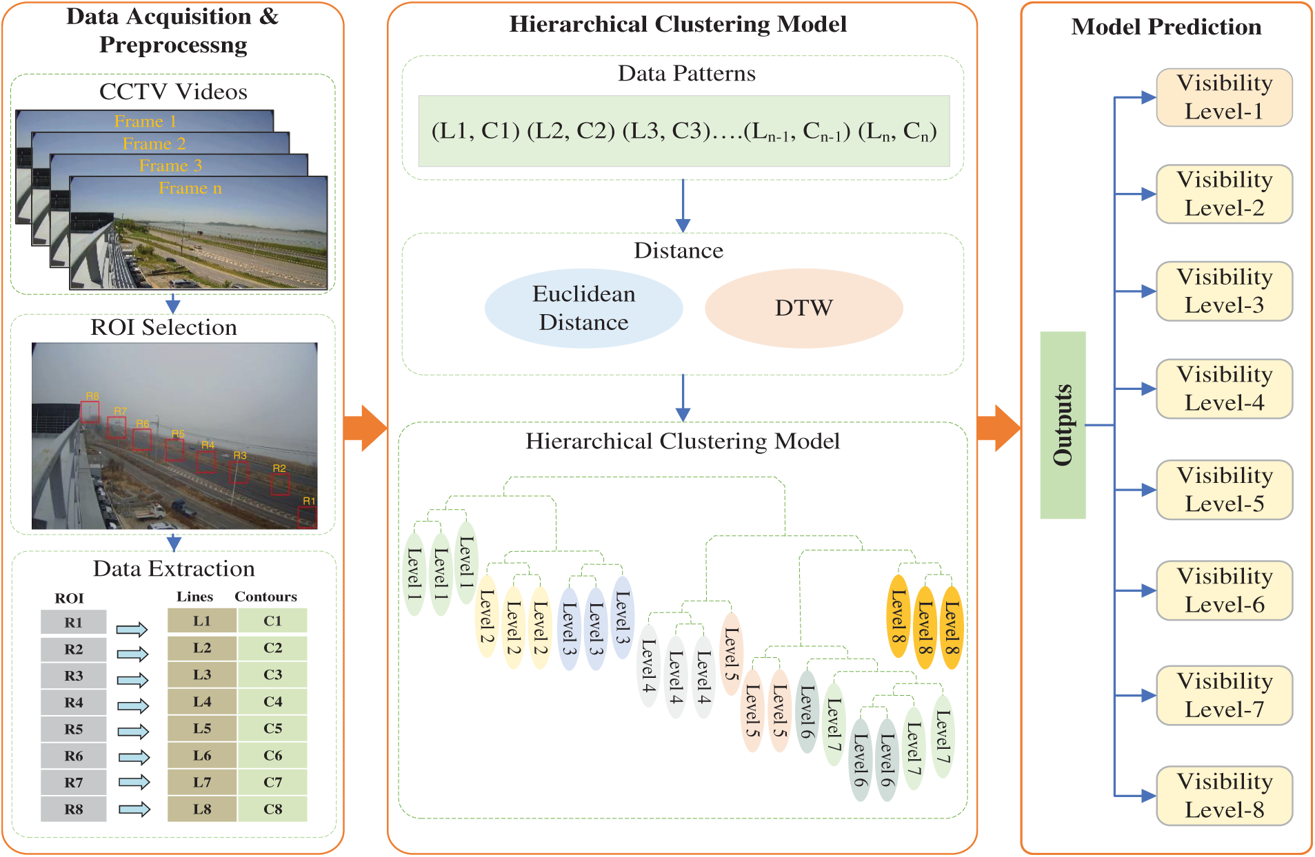
Figure 1: Proposed framework for visibility classification using ROI-based feature extraction and clustering

3.1 Data Preprocessing

To classify CCTV images effectively, preprocessing and feature extraction are essential for differentiating visibility levels. First, we extract frames from the videos and fix ROIs within each frame (see the first part of Fig. 1). Since weather conditions do not change rapidly, processing every frame is unnecessary. Therefore, we choose one frame every 30 s from the video, either by random selection or by averaging features from ten randomly chosen frames. Given that CCTV videos record at 30 fps, this means selecting ten frames out of 900 and computing their average feature values. This workflow is outlined in Algorithm 1.

In the next step, we focus on ROIs rather than the entire image to reduce computational cost and improve feature quality. Road is ideal for selecting ROIs because it has a consistent texture across cameras and provides reliable data patterns for visibility assessment. Through extensive testing, we determined the optimal ROI size, which we discuss further in the evaluation Section 4.2.

3.2 Feature Extraction

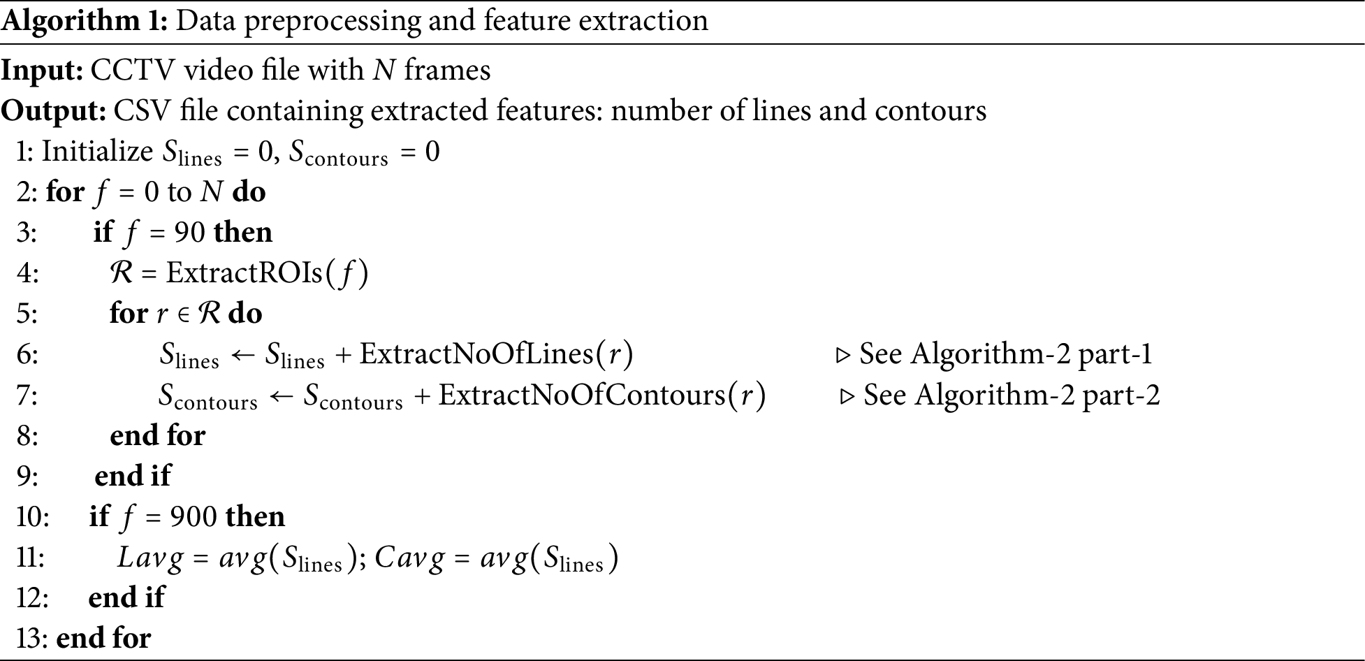
For feature extraction, first ROIs were manually selected, for which we used a distance meter to measure the real-world distance of identifiable fixed objects visible within each CCTV frame. These measured distances are then used to define consistent ROI regions along the field of view to enable reliable visibility estimation. From each ROI, we extract two features: the number of lines and the number of contours. This process helps us create a data pattern that differentiates images with varying visibility levels. The whole process is explained in Algorithm 1, which takes a video file as input and gives a CSV file as output containing the extracted feature values. Line 1 initializes the variables, lines 2 to 11 loop through the video file and extract the features from every 90th frame, and lines 10 to 12 store the final average values for every 30 s. Further details of feature extraction are given below.

3.2.1 Extraction of Feature 1 (Number of Contours)

The first feature we have focused on is detecting and calculating the number of contours. A contour is a curve that connects continuous points of the same colour or intensity within an image. Contours are particularly useful for analyzing shapes in an image. We chose the number of contours as a feature because it effectively helps differentiate images with varying visibility levels.

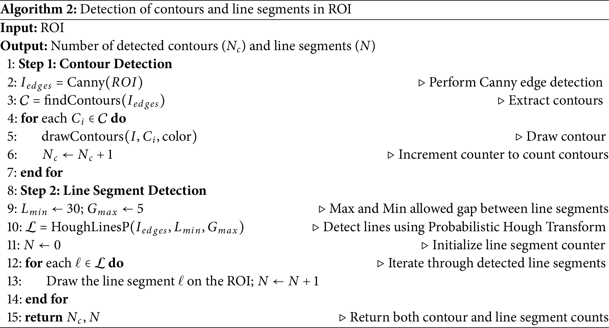
Fig. 2a illustrates the contours detected within each ROI, with each contour shown in a different colour. In Algorithm 2, step 1 processes ROIs to detect and count the number of contours. First, the algorithm uses Canny edge detection to detect the edges within the blurred image, as shown on line 2. After the edge detection, it detects the contours (object boundaries) in the image. It then draws each contour on the original ROI and keeps a count of how many contours are found. Finally, the algorithm returns the total number of contours detected. This approach is useful for finding and analyzing shapes in a specific part of an image.

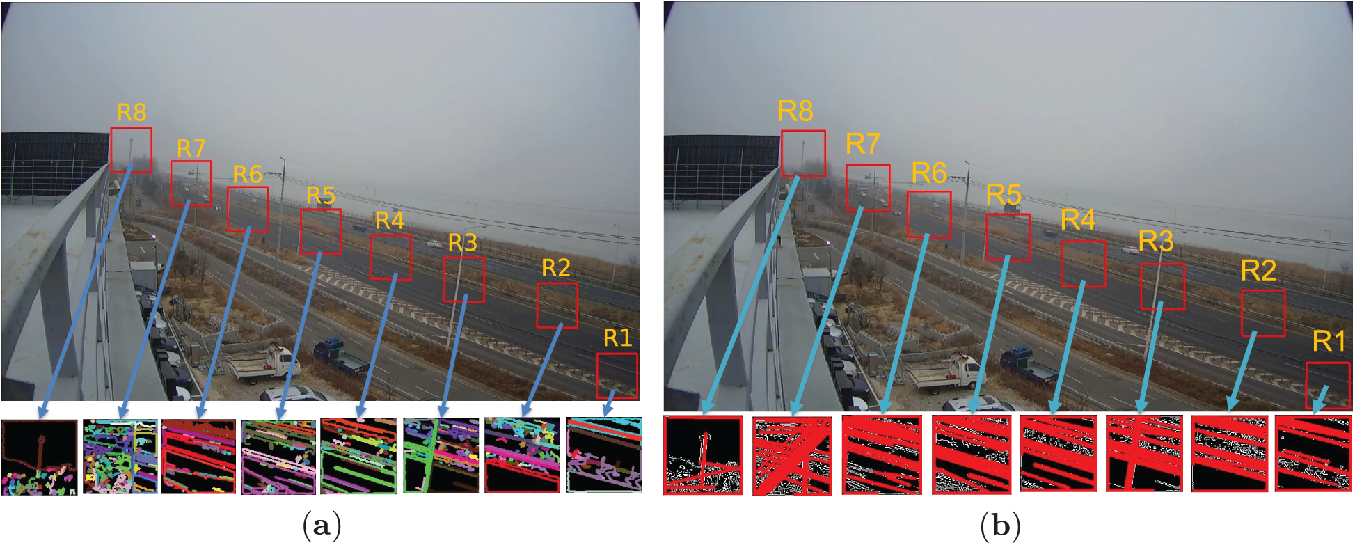
Figure 2: Feature extraction from ROIs (a) Number of Contours (b) Number of Lines

3.2.2 Extraction of Feature 2 (Number of Lines)

For the second feature, we extracted the number of lines found within each ROI. The OpenCV library in the C++ programming language was used to count these lines. The probabilistic Hough line transform is applied, which detects lines by counting the number of intersections between curves. Fig. 2b shows an example of the detected lines within each ROI and are highlighted in red. We count these lines for each ROI, and they are considered the final feature value.

Algorithm 2 step 2 detects and counts the number of lines in ROIs. It starts by setting two parameters: the minimum line length (30 pixels) and the maximum gap between parts of a line (5 pixels), at line 9. These settings help define what will be recognized as a line. Next, it applies the Hough Transform method to find lines in the edge-detected image based on the earlier settings. The algorithm goes through each detected line, drawing it on the original ROI and keeping a count of the lines found. Finally, it returns the total detected number of lines.

3.3 Proposed Hierarchical Clustering-Based Learning Model

We developed a hierarchical clustering model to classify the images based on the data patterns identified in the previous section. This model groups similar images together by analyzing the extracted features, such as the number of lines and contours, allowing for effective categorizaion under different visibility circumstances.

3.3.1 Learning Model

Hierarchical clustering follows a bottom-up approach. It is very straightforward to implement and allows us to avoid threshold-based methods by providing learning capabilities on relatively small and diverse datasets. During this process, images with the same fog intensity are grouped into the same cluster.

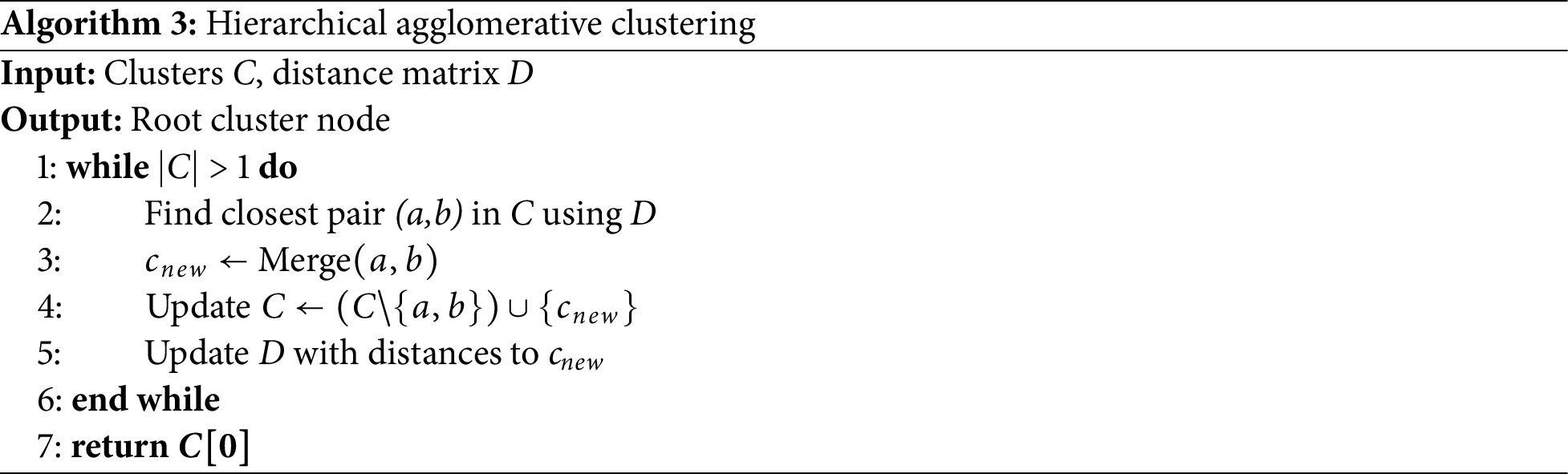
Our proposed model begins with the data patterns explained in the previous section. As is shown in Algorithm 3, each pattern is initially treated as a separate cluster, then it computes a distance matrix to measure similarities between patterns, with shorter distances indicating higher similarity. The two most similar clusters are then merged, and the distance matrix is updated iteratively. This process repeats, progressively building a hierarchical tree structure, until only a single cluster remains, representing the root of the hierarchical tree. We have used average linkage (UPGMA) for its balanced cluster variance handling and set the 0.85 cutoff threshold through empirical optimization, maximizing silhouette scores while maintaining eight distinct visibility clusters.

3.3.2 Distance Matrix

Calculating the similarity distance between data patterns is an important step in implementing the hierarchical clustering. Various similarity metrics can be used to compute these distances, such as Euclidean distance or DTW. The process involves comparing all clusters to each other using the selected distance metric and storing the calculated results in the matrix. This distance matrix is crucial for understanding the relationships between clusters. The distance metrics we experimented with, Euclidean and DTW, are described in detail in the following sections.

Dynamic Time Warping (DTW) Distance

DTW is usually used to find the similarity or optimal alignment between two time series sequences. It is non-linear in nature and is a commonly used technique in pattern recognition and sequence alignment. We chose it to calculate the similarity between data patterns because its warping process increases the accuracy of similarity. It can be represented mathematically as follows:

DTW(T,Q)={∑i=1mdist(t1,qi)if (n=1)∑j=1ndist(tj,q1)if (m=1)dist(tn,qm)+min{DTW(Tn−1,Qm−1)DTW(Tn−1,Qm)DTW(Tn,Qm−1)Otherwise(1)

Eq. (1) defines the DTW distance between two sequences T={t1,…,tn} and Q={q1,…,qm}. It recursively computes the optimal alignment by minimizing the cumulative distance dist(ti,qj), considering insertion, deletion, and match operations. Fig. 3 illustrates how DTW is used to calculate the similarity between two patterns. In the first step of this process, a point table is generated using the Euclidean distance between all possible pairs of the input pattern. In the next step, a DTW table is generated using Eq. (1), the value at the bottom right corner represents the similarity distance.

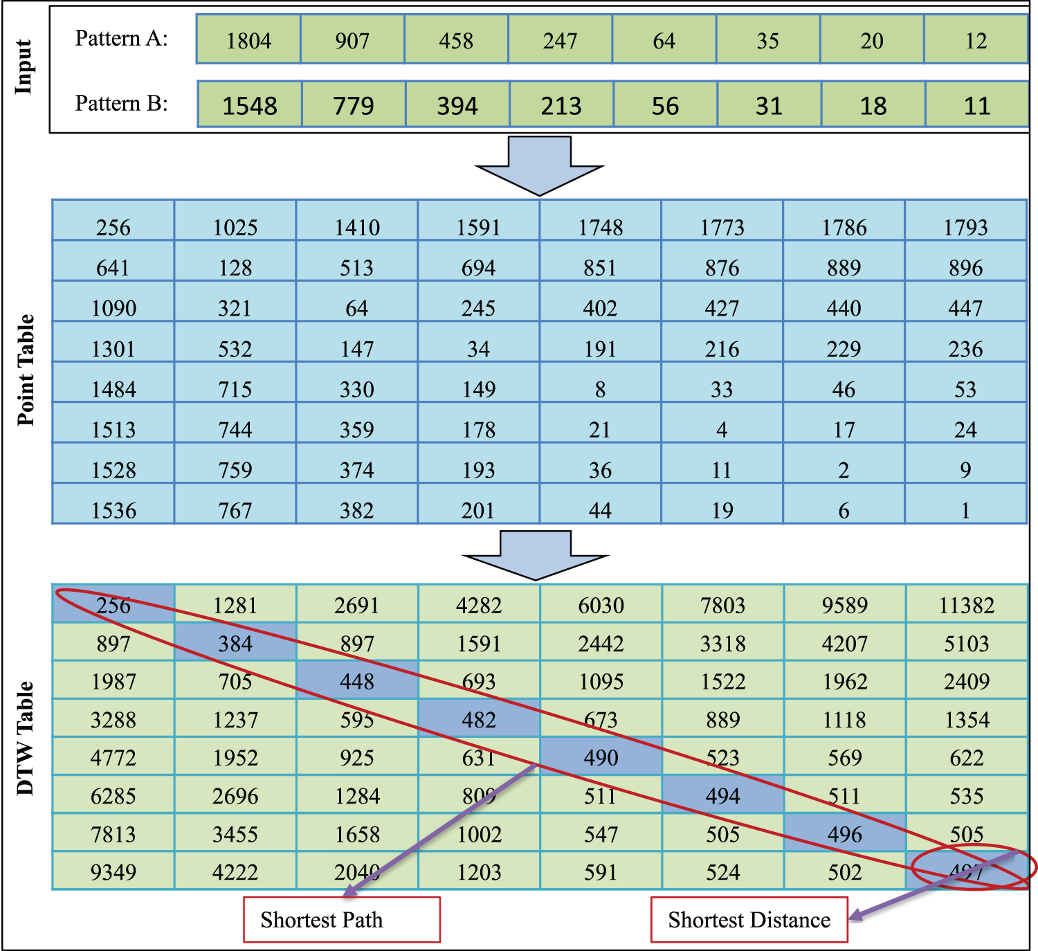
Figure 3: Calculating similarity value between two sequence patterns using DTW

Minkowski Distance

Minkowski distance is another metric commonly used to measure similarity distance between data patterns, shown in Eq. (2). The parameter p determines the type of distance metric: if p=1, it becomes the Manhattan distance, given by DMan(X,Y)=∑i=1n|xi−yi|. If p=2, it simplifies to the Euclidean distance, defined as DEuclidean(X,Y)=(∑i=1n(xi−yi)2)12. If p→∞, it becomes the Chebyshev distance, it is expressed as DChebyshev(X,Y)=maxi|xi−yi|. Thus, p controls how the differences between coordinates are aggregated. We have experimented with different p values, the results of p=2,p=4 which p=10 are selected and presented in Section 4.1. Euclidean distance is used as a baseline for comparison with DTW. The key difference is that DTW is a non-linear method, while Euclidean distance (a form of Minkowski) is linear in nature.

DMinkowski(X,Y)=(∑i=1n|xi−yi|p)1p(2)

3.3.3 Prediction Using Hierarchical Tree

After implementing hierarchical clustering, we create a prediction model using the resulting tree structure. Fig. 4 shows how this model works: a new CCTV image is provided as input, and a data pattern is extracted from it. We then compare this pattern with each sub-cluster in the hierarchical tree to find the closest match. The visibility level of the image is predicted based on the common label in the most similar sub-cluster.

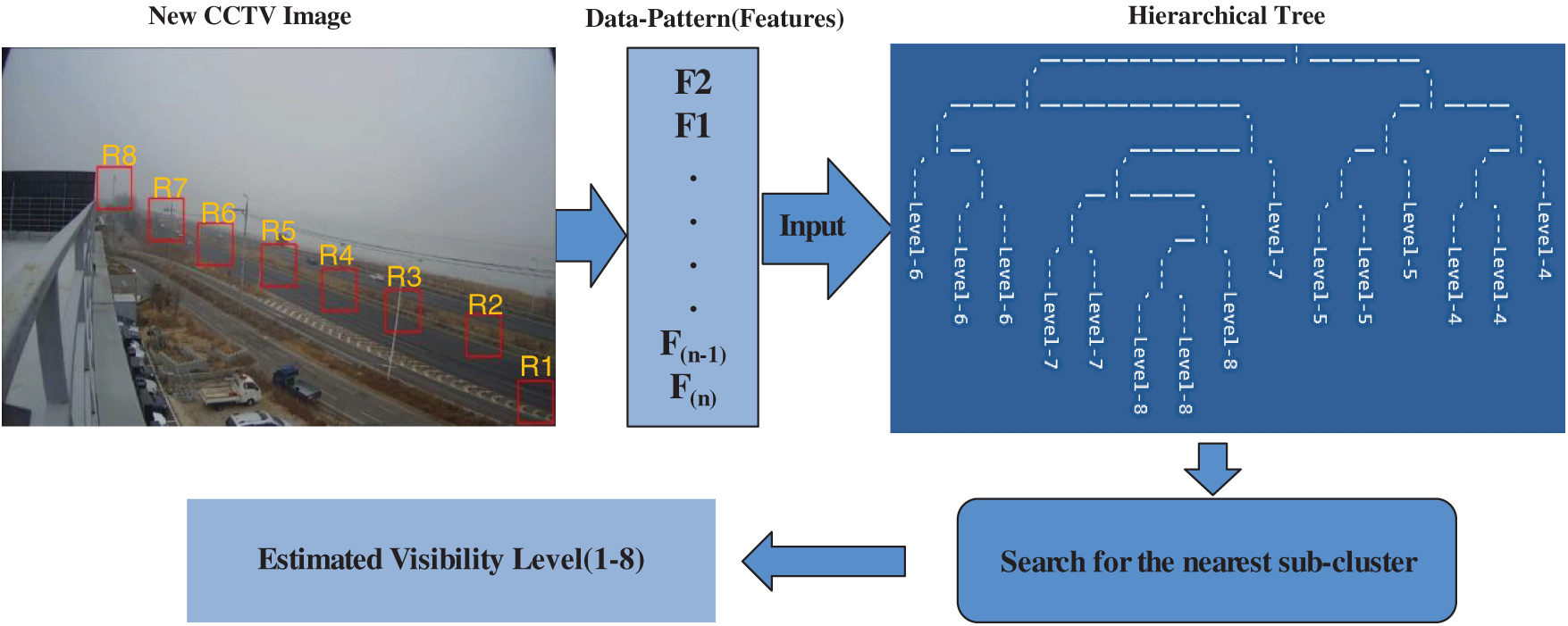
Figure 4: Predicting the visibility level using the hierarchical clustering model

4  Results and Evaluations

In this section, we evaluate the performance of our proposed method using real-time datasets collected from roadside CCTV cameras under diverse visibility conditions. First, we analyzed the key features, like the number of contours and lines, and then compared the performance of our proposed model with DL approaches. All these experiments, including feature extraction, hierarchical tree creation, and evaluations, were performed using the OpenCV library (version 3.4.11) in C++ [35]. The results highlight the robustness and consistency of our model, especially in handling diverse data from different locations. The following sections provide a more detailed discussion of dataset collection, preprocessing, and simulation outcomes.

4.1 Dataset

Problem-specific and authentic datasets play a key role in the development of intelligent AI-based systems. Keeping this in mind, we collected a real-time dataset using the CCTV cameras fixed at the roadsides and then divided it into two parts, where one is used for training while the other is used for testing of the model. The data collection was supported by the Database and Big Data Lab of Pusan National University [36]. The data was collected from six different roadside cameras; three cameras were set up in Busan City, while the other three were set up in Seoul City. The data was collected from March 2018 till April 2019, with its size exceeding 200 GB. Each image is of resolution 1080 × 1920. The videos were extracted only for daytime, and a 5-min video clip was stored for every hour. It contains around 20 days of low-visibility weather conditions, including heavy rain, snow, and fog. A total of 7000 images were extracted, out of which 1920 images were used for evaluations, keeping an equal number of images for each visibility level to keep the dataset balanced. Fig. 5 shows example images for eight different visibility levels, where level-1 indicates the highest visibility while level-8 represents the lowest visibility. These visibility levels are labelled manually based on human perception and the weather forecast from the official website1. This careful curation ensures that the dataset is representative of various weather scenarios, allowing for more robust analysis and model training.

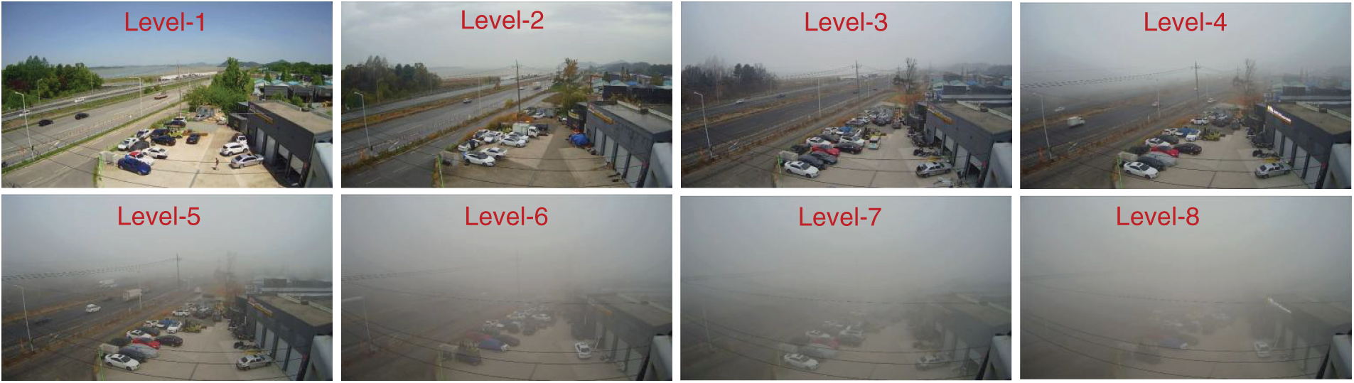
Figure 5: Examples of CCTV images labelled with eight different visibility levels

4.2 Evaluation of Different ROI Sizes

Choosing the best ROI size is of great significance for better feature extraction, having direct implications for its ability to classify. Therefore, we used images with four different sizes (in pixels) of ROIs, such as 160 × 160, 120 × 120, 80 × 80, and 40 × 40. We then evaluate the results attained via different ROI sizes in terms of the number of lines to select the optimum ROI size. The experimental results for four different ROI sizes for the number of lines are shown in Fig. 6, where three different weather conditions are compared. Fig. 6a shows that for each ROI and weather condition, there is no significant pattern, but as the size of ROI increases (shown in Fig. 6b–d) we can find a clear pattern of differentiating different weather conditions (especially ROI size 160 × 160). Similarly, we evaluate the results for four different ROI sizes for the number of contours. According to the simulation results, the ROI size of 160 × 160 was the best among the selected sizes. Therefore, we choose 160 × 160 as the best ROI and have used it for all of the experimental work.

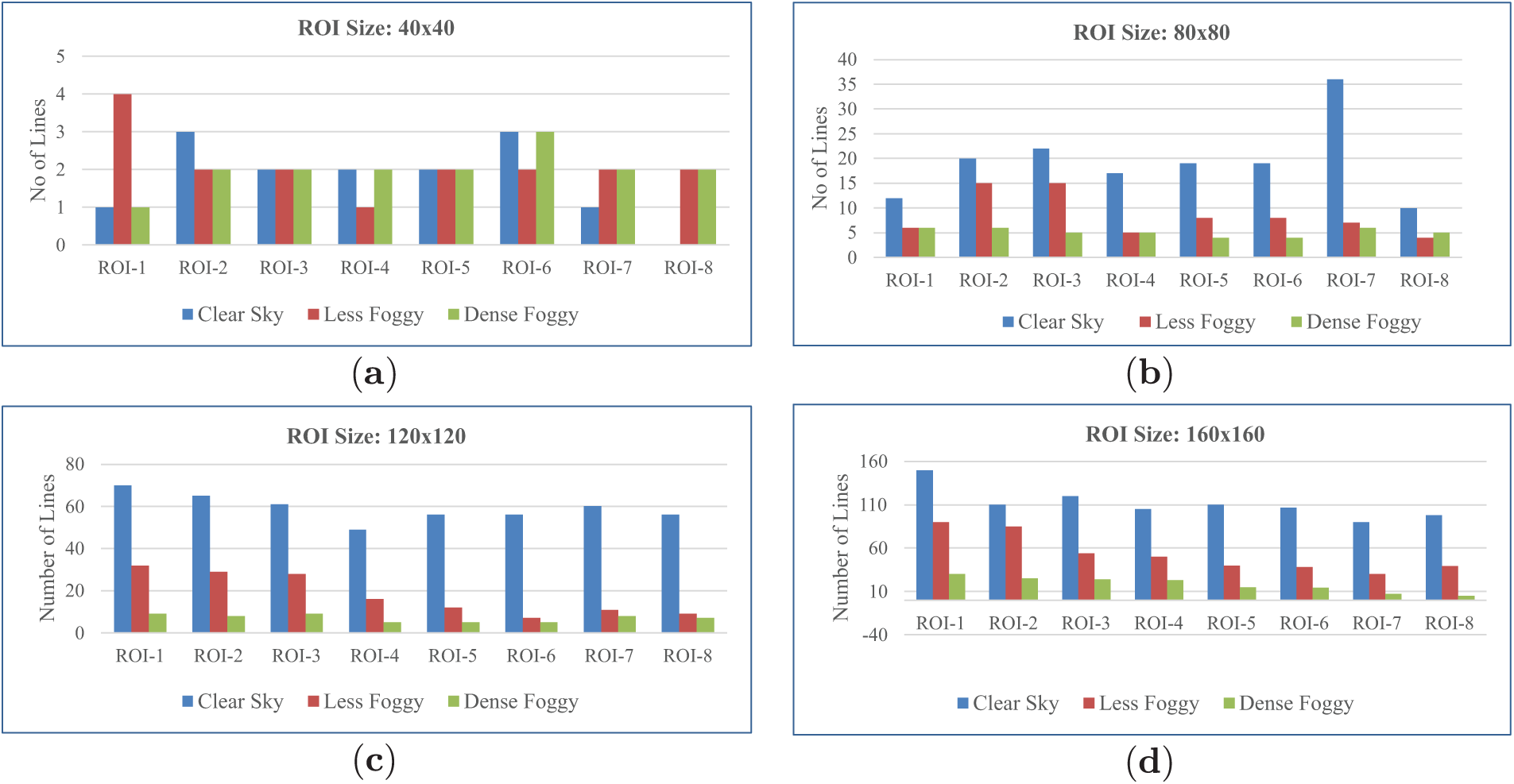
Figure 6: Effect of ROI size on line pattern detection for weather classification under different conditions

4.3 Impact of Image Resolution

To evaluate how image resolution affects feature extraction accuracy, we conducted multiple experiments using downsampled versions of the original 1080p (1920 × 1080) CCTV images. Four step-by-step lower resolutions were tested: 720p (1280 × 720), 540p (960 × 540), 360p (640 × 360), and 180p (320 × 180), maintaining the optimal 160 × 160 ROI size determined in Section 4.2. The analysis results revealed significant resolution-dependent effects for lines and contours. As shown in Fig. 7, line detection is degraded by 18.7% at 720p and 63.2% at 180p due to the loss of fine edge details, while contour detection showed greater sensitivity with a 32.4% reduction at 720p and 81.1% at 180p. Visibility discrimination remained reasonable down to 540p resolution but deteriorated substantially below 360p. For implementation, we used Lanczos resampling for better quality during downsampling, maintained physical ROI locations using camera calibration data, and implemented scale-adaptive thresholds using the following formula:

τnew=τbase×Wcur×HcurWorig×Horig(3)

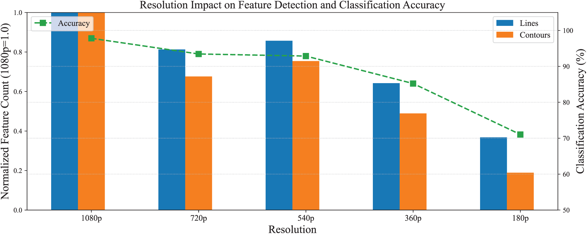
Figure 7: Resolution impact on feature detection accuracy (normalized to 1080p baseline)

In the above equation, τbase illustrate the original threshold at 1080p resolution. This resolution analysis revealed that adaptive downsampling (e.g., Lanczos for high-contrast regions) could reduce processing time at 540p with minimal loss, making it viable for embedded systems. This approach balances resource constraints and feature retention.

4.4 Performance under Combined Extreme Conditions

To evaluate robustness under simultaneous adverse conditions, we analyzed images exhibiting both heavy rain and dense fog. These conditions represent the most challenging scenarios in the dataset. Using the optimal 160 × 160 ROI size and DTW-based clustering, we achieved a precision of 89.7% and recall of 88.3% (Table 1), demonstrating consistent performance degradation of only 1.4% compared to single-condition fog. This marginal decline highlights the model’s resilience and is given as follows:

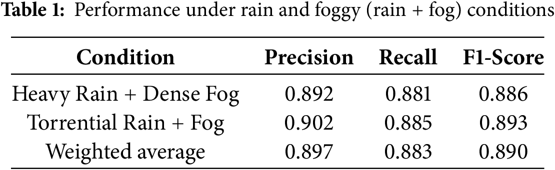
•   Feature Complementarity: Contour detection remains effective in heavy rain (preserving edge structures), while line features maintain discriminative power in dense fog.

•   DTW Adaptation: Non-linear warping accommodates irregular feature distortion patterns during co-occurring precipitation and fog.

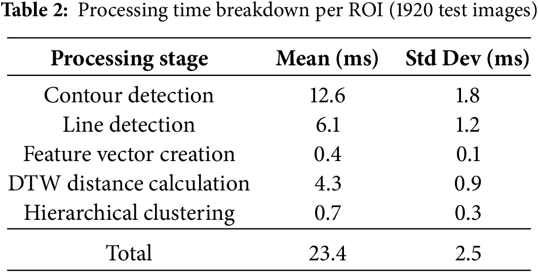
4.5 Scalability and Latency Analysis

To evaluate the real-time performance of the model, we measured its processing time using a system with an Intel Core i7 CPU (3.60 GHz) and 32 GB RAM. Table 2 shows the average processing time per ROI across different stages. The complete pipeline processes one ROI in 23.4 ms (mean), enabling real-time operation at 42.7 frames per second. Contour detection was the most computationally intensive stage (12.6 ms), while clustering required only 0.7 ms.

We further evaluated the system scalability by increasing the camera counts (1–50 cameras), considering 5-min video segments. The results show near-linear scaling up to 20 cameras (42.3 s total processing time). At 50 cameras, processing required 106.7 s, indicating that distributed processing is needed for large deployments. This demonstrates that our system can handle 10–20 cameras in real-time on a single workstation. Furthermore, the energy consumption average rate was 0.21 Wh/frame under sustained load (measured via Intel RAPL), translating to 9 W at 42.7 fps. This efficiency enables deployment on edge devices (e.g., Jetson AGX Xavier: 30 W TDP) without hardware modifications.

4.6 Features Evaluation

In order to classify visibility across various ROIs and weather situations, this section assesses the discriminative power of two essential features: the number of contours and the number of lines. Both of the features are evaluated for different ROIs and weather conditions.

The association between visibility levels and contour counts for eight ROIs is shown in Fig. 8a. The x-axis indicates the ROI distance from the CCTV camera, whereas the y-axis illustrates contour counts. The findings show a strong positive connection, with more variance and contour counts under high-visibility (clear sky) situations than in low-visibility ones. The feature’s robustness for categorization is confirmed by the clear division between visibility classes. DTW’s ability to adapt to temporal differences through non-linear sequence alignment makes it more resistant against changes in speed and data shifts, which is why it works well under such situations.

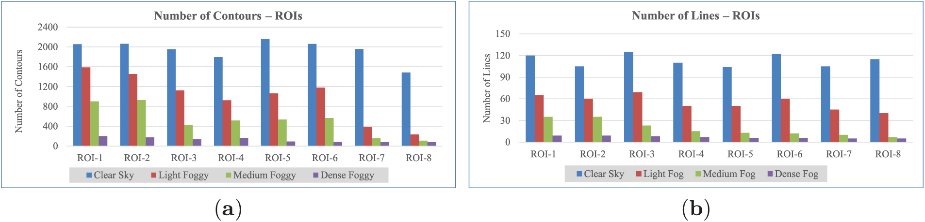
Figure 8: Features’ ability to differentiate visibility levels (a) Number of Contours (b) Number of Lines

Fig. 8b further explains these findings through analysis of line detections at varying visibility levels. In accordance with contour-based observations, increased visibility levels result in a significantly greater number of detected lines. These features collectively create a pattern that effectively distinguishes visibility levels in CCTV imagery. We can conclude that both features effectively create a strong data pattern for distinguishing between different visibility levels in images.

4.7 Similarity Distance Metrics Evaluations

Table 3 presents the performance evaluation of hierarchical clustering using two different distance metrics: DTW and Euclidean distance, while its respective confusion matrices are given in Fig. 9a and b. The results are reported in terms of accuracy, precision, recall, and F1 score for each class separately (Level 1 to Level 8).

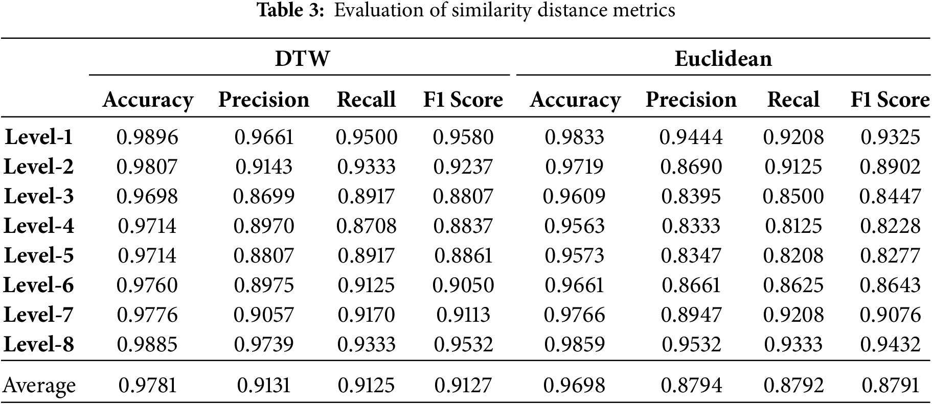
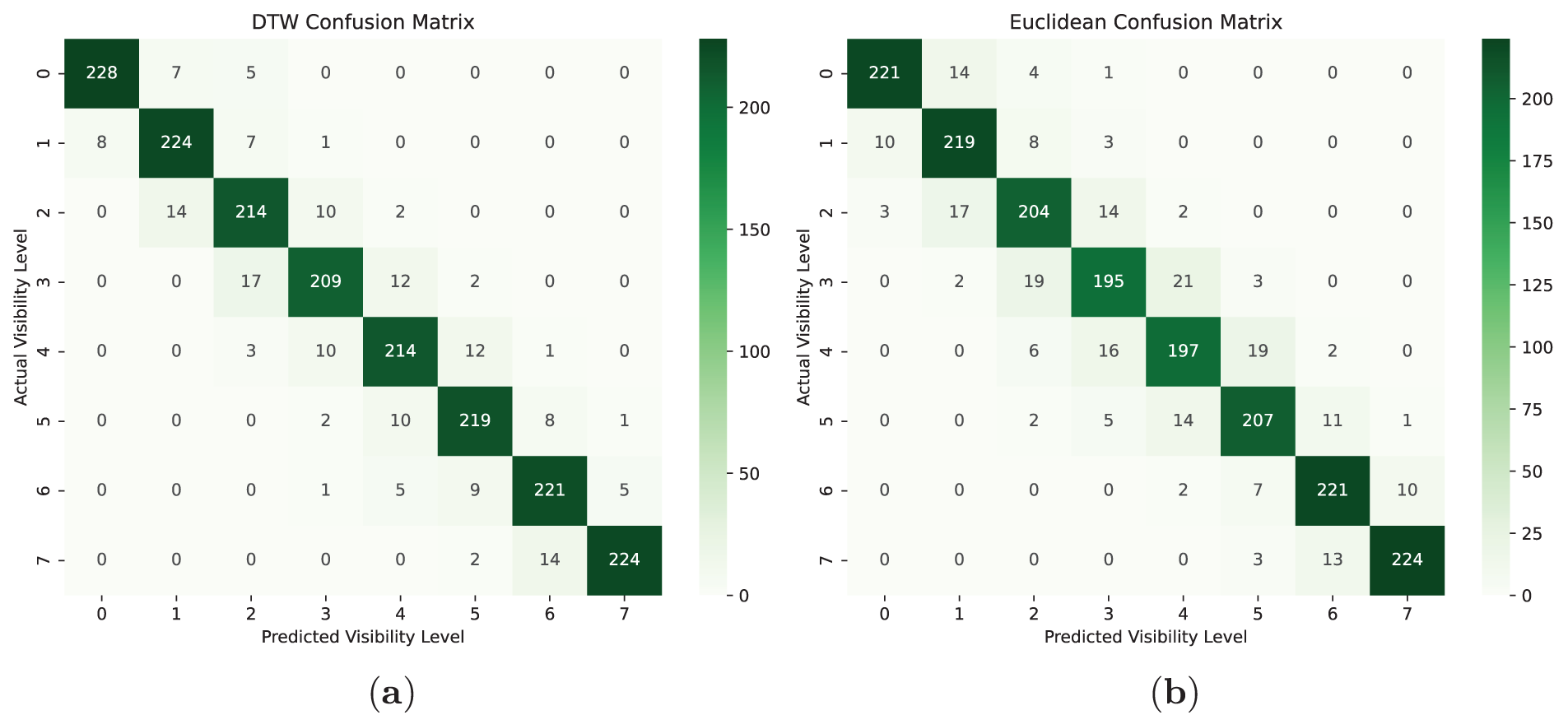
Figure 9: Confusion matrix of similarity distance metrics: (a) DTW (b) Euclidean

It is evident that the DTW-based clustering outperforms the Euclidean-based approach across all metrics. DTW achieves a higher average accuracy (0.9781 vs. 0.9698), precision (0.9131 vs. 0.8794), recall (0.9125 vs. 0.8792), and F1 score (0.9127 vs. 0.8791). The superior performance of DTW can be attributed to its ability to handle temporal distortions and align sequences more effectively, making it more suitable for time-series clustering tasks. These results suggest that DTW is a more robust distance metric for hierarchical clustering in this context.

4.8 Clustering Evaluations and Comparisons with Deep Learning

In this section we present a thorough comparison of our proposed model with numerous DL models used in the literature. We assessed our model from various perspectives, including similarity metrics, features, and data location. Table 4 shows the experimental results attained using the data collected from cameras located in the same location. For combined data (collected from cameras located in two different locations), DTW achieved the highest precision at 91%, while the Euclidean metric had the highest precision of 87% and the lowest at 83%.

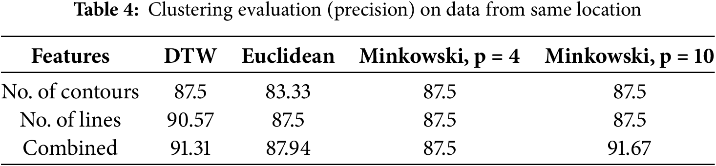
Table 5 illustrates the precision of hierarchical clustering on data collected from different locations, meaning the data was gathered from cameras installed at different roadside locations. In this experiment, DTW again performed better, having a precision of 90%, while Euclidean had the highest precision of 86%.

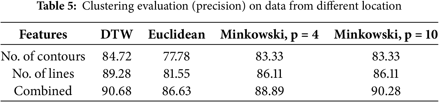
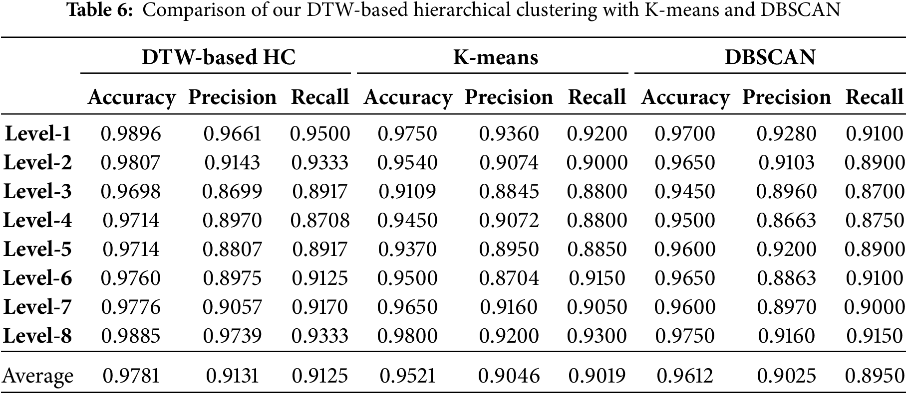
Table 6 presents a thorough comparison of the performance of our proposed model with K-means and DBSCAN (density-based spatial clustering of applications with noise) across various evaluation metrics (accuracy, precision, and recall) at different visibility levels. The The proposed DTW-based HC model consistently outperforms both K-means and DBSCAN, achieving higher accuracy, precision, and recall across all visibility levels. The average accuracy (0.9781) and precision (0.9131) for DTW-based HC are superior to those of both K-means and DBSCAN, which have average accuracies of 0.9521 and 0.9612, respectively. Our approach performs well because of its ability to capture temporal patterns and similarities, outperforming K-means and DBSCAN, which struggle with non-linear patterns and varying clusters.

Besides K-means and DBSCAN, we also compared our proposed approach with state-of-the-art DL models, including YOLOv5 (fine-tuned on our dataset) and a Multilayer Perceptron (MLP). For MLP, the layer configuration consists of an input layer, an output layer, and three hidden layers. The input is the image of ROI of size 128 × 128; the initial learning rate is 0.01, the maximum number of learning repetitions is 100, and the learning time required is 11 min 31 s. Fig. 10a shows the confusion matrix for the MLP using data from the same location (precision: 87.4%). Fig. 10b presents the confusion matrix for data from different locations, with a precision of 84.63%. YOLOv5 achieved 89.2% precision on same-location data but dropped to 83.1% on different locations, as shown in Table 7, while our proposed model achieved 91.3% and 90.7%, respectively. This demonstrates our method’s superior performance and robustness to location variation compared to DL approaches.

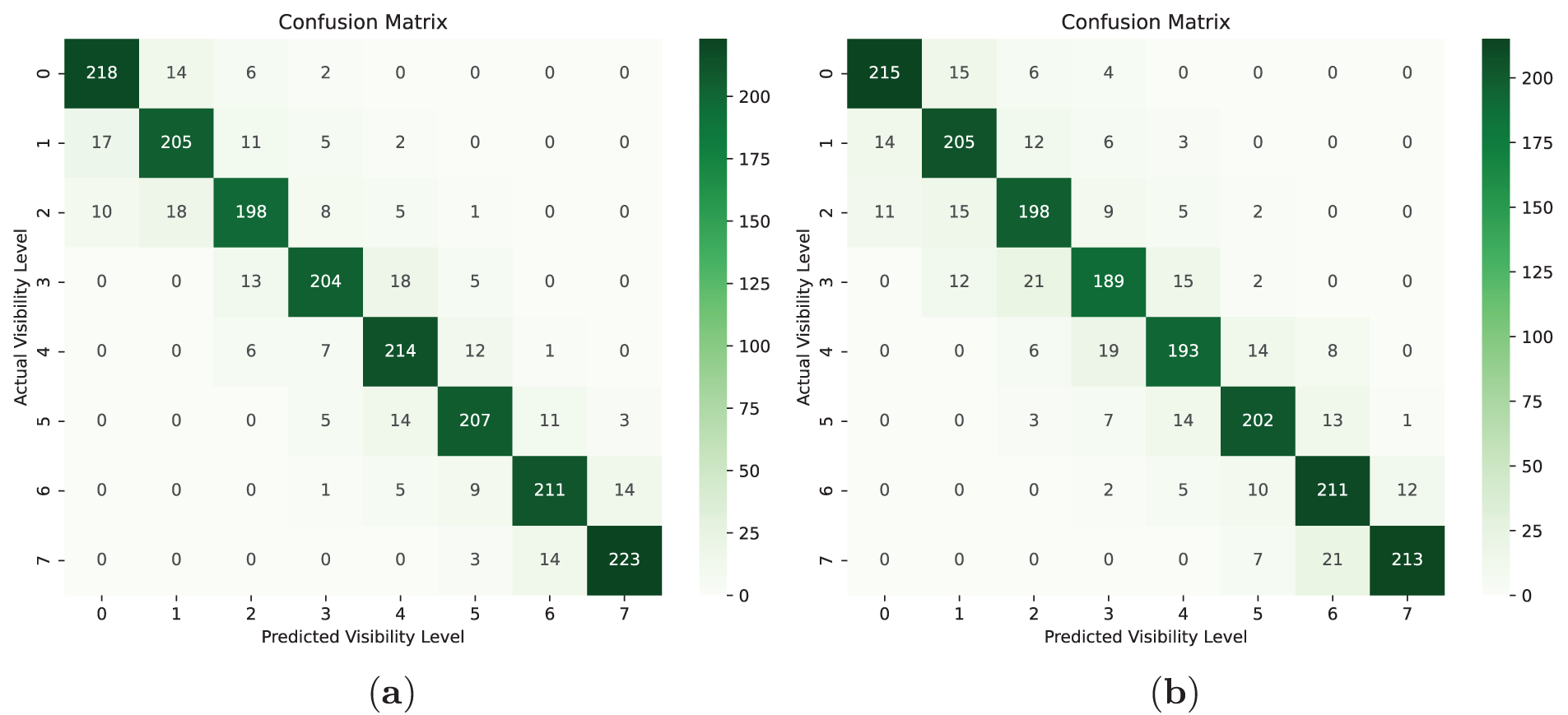
Figure 10: Confusion matrix of DL model: (a) same location data; (b) different location data

The simulation results show that our proposed approach outclassed all other methods in terms of numerous performance measures, demonstrating its generalizability, robustness, and consistency for identifying different visibility levels under diverse weather conditions and case scenarios.

5  Conclusion

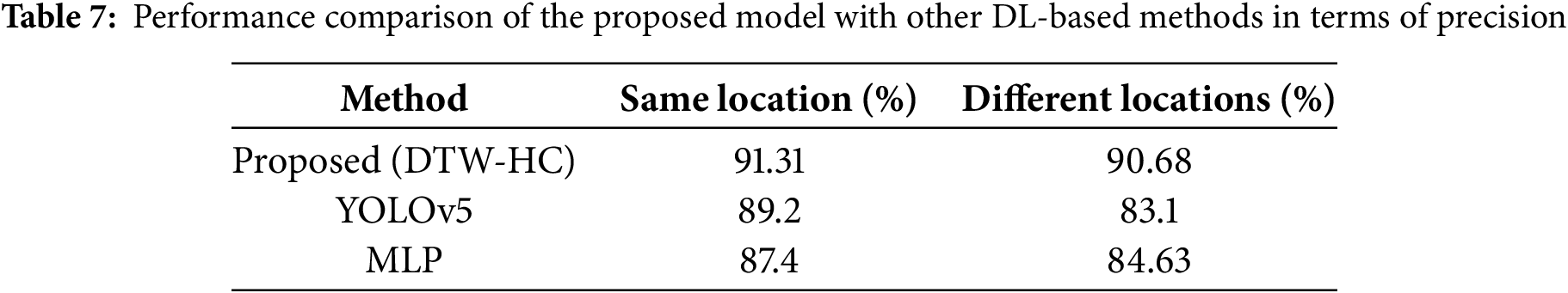
In this study, we proposed a hierarchical clustering-based learning model to estimate road visibility using images from roadside CCTV cameras installed for surveillance purposes. Our approach begins by extracting data patterns from the CCTV footage of cameras installed at roadsides. We focused on a specific ROI in the images and extracted two key features: the number of lines and contours. These features form the basis of our data pattern, which is then used as an input for the hierarchical clustering model to classify the data and estimate the visibility level. A critical aspect of our hierarchical clustering process is the calculation of the distance matrix, which measures the similarity between patterns. We employed two similarity metrics for this purpose: DTW and the Minkowski distance metric. During the evaluation, we compared the results of both metrics and found that DTW outperformed Minkowski, achieving the highest accuracy of 97.81%. Furthermore, we compared our proposed model with DL-based models, which proves the significance and versatility of the proposed approach. Our model achieved 91.31% precision for samples collected from the same location and 90.68% precision for instances collected from different locations. In contrast, the DL-based model achieved 87.4% precision using the same location data and 84.63% precision for the data collected from different locations. Based on these results, we conclude that our approach not only delivers higher overall results but also performs better on diverse datasets.

The potential future work of this study includes experimenting with more similarity distance metrics, such as Mahalanobis, and additional features, such as histograms of color intensity or unsupervised/semi-supervised ML-based representations, to enhance the efficiency of the visibility estimation system. In addition, exploring other advanced clustering methods or hybrid approaches can further improve the performance. Furthermore, our model generalizes across urban settings; extending it to extreme environments (e.g., the Arctic, deserts) would require specialized datasets and sensor adaptations. Therefore, validating the model on a huge and more diverse dataset, including the data collected from a large number of cameras with different camera perspectives (resolutions, angles, etc.), will further enhance its generalizability and robustness for real-world applications.

Acknowledgement: We extend our appreciation to all the authors for their hard work, continuous support, and encouragement to accomplish this research work in a friendly and professional environment.

Funding Statement: This paper recieves no financial support.

Author Contributions: The authors confirm contribution to the paper as follows: Conceptualization, Asmat Ullah and Yar Muhammad; methodology, Asmat Ullah and Bakht Zada; software, Asmat Ullah and Yar Muhammad; validation, Korhan Cengiz, Nikola Ivković and Mario Konecki; formal analysis, Abid Yahya and Bakht Zada; investigation, Yar Muhammad; resources, Asmat Ullah and Abid Yahya; data curation, Asmat Ullah; writing, Asmat Ullah and Yar Muhammad; writing—review and editing, Asmat Ullah and Yar Muhammad; visualization, Bakht Zada and Abid Yahya; supervision, Asmat Ullah and Korhan Cengiz; project administration, Asmat Ullah; funding acquisition, Nikola Ivković and Mario Konecki. All authors reviewed the results and approved the final version of the manuscript.

Availability of Data and Materials: The data used in this study is available from the corresponding authors upon special request.

Ethics Approval: Not applicable.

Conflicts of Interest: The authors declare no conflicts of interest to report regarding the present study.

1Korea Meteorological Administration: https://www.kma.go.kr/ (accessed on 21 July 2025).

References

1. Sun G, Zhang Y, Yu H, Du X, Guizani M. Intersection fog-based distributed routing for V2V communication in urban vehicular ad hoc Networks. IEEE Trans Intell Transp Syst. 2020;21(6):2409–26. doi:10.1109/TITS.2019.2918255. [Google Scholar] [CrossRef]

2. Sun Y, Tang J, Liu Q, Zhang Z, Huang L. Highway visibility level prediction using geometric and visual features driven dual-branch fusion network. IEEE Trans Intell Transp Syst. 2024;25(8):9992–10004. doi:10.1109/TITS.2024.3362905. [Google Scholar] [CrossRef]

3. You J, Jia S, Pei X, Yao D. DMRVisNet: deep multihead regression network for pixel-wise visibility estimation under foggy weather. IEEE Trans Intell Transp Syst. 2022;23(11):22354–66. doi:10.1109/TITS.2022.3180229. [Google Scholar] [CrossRef]

4. Li L, Ahmed MM. A deep learning approach for multiple weather conditions detection based on in-vehicle dash camera video. In: Proceedings of the International Conference on Transportation and Development 2024. Reston, VA, USA: American Society of Civil Engineers; 2024. doi:10.1061/9780784485514.04. [Google Scholar] [CrossRef]

5. Li M, Wang G. A method combining mobile transmissometer and Lidar for high precision measurement of visibility. IEEE Photonics J. 2024;16(4):1–10. doi:10.1109/JPHOT.2024.3410293. [Google Scholar] [CrossRef]

6. Liang J, Yang K, Tan C, Wang J, Yin G. Enhancing high-speed cruising performance of autonomous vehicles through integrated deep reinforcement learning framework. IEEE Trans Intell Transp Syst. 2025;26(1):835–48. doi:10.1109/TITS.2024.3488519. [Google Scholar] [CrossRef]

7. Gao Y, Xu W, Lu Y. Let you see in Haze and Sandstorm: two-in-one low-visibility enhancement network. IEEE Trans Instrum Meas. 2023;72:1–12. doi:10.1109/TIM.2023.3304668. [Google Scholar] [CrossRef]

8. Yang W, Zhao Y, Li Q, Zhu F, Su Y. Multi visual feature fusion based fog visibility estimation for expressway surveillance using deep learning network. Expert Syst Appl. 2023;234:121151. doi:10.1016/j.eswa.2023.121151. [Google Scholar] [CrossRef]

9. Pal T, Halder M, Barua S. A deep learning model to detect foggy images for vision enhancement. Imaging Sci J. 2023;71(6):484–98. doi:10.1080/13682199.2023.2185429. [Google Scholar] [CrossRef]

10. Boudala FS, Gultepe I, Milbrandt JA. The performance of commonly used surface-based instruments for measuring visibility, cloud ceiling, and humidity at Cold Lake, Alberta. Remote Sens. 2021;13:5058. doi:10.3390/rs13245058. [Google Scholar] [CrossRef]

11. Liu X, Zhou X. Determinants of carbon emissions from road transportation in China: an extended input-output framework with production-theoretical approach. Energy. 2025;316:134493. doi:10.1016/j.energy.2025.134493. [Google Scholar] [CrossRef]

12. Peng X, Song S, Zhang X, Dong M, Ota K. Task offloading for IoAV under extreme weather conditions using dynamic price driven double broad reinforcement learning. IEEE Internet Things J. 2024;11(10):17021–33. doi:10.1109/JIOT.2024.3360110. [Google Scholar] [CrossRef]

13. Li J, Lo WL, Fu H, Chung HSH. A transfer learning method for meteorological visibility estimation based on feature fusion method. Appl Sci. 2021;11(3):997. doi:10.3390/app11030997. [Google Scholar] [CrossRef]

14. Guo Y, Liu RW, Lu Y, Nie J, Lyu L, Xiong Z, et al. Haze visibility enhancement for promoting traffic situational awareness in vision-enabled intelligent transportation. IEEE Trans Veh Technol. 2023;72(12):15421–35. doi:10.1109/TVT.2023.3298041. [Google Scholar] [CrossRef]

15. Kim KW. The comparison of visibility measurement between image-based visual range, human eye-based visual range, and meteorological optical range. Atmos Environ. 2018;190:74–86. doi:10.1016/j.atmosenv.2018.07.020. [Google Scholar] [CrossRef]

16. Yang L, Muresan R, Al-Dweik A, Hadjileontiadis LJ. Image-based visibility estimation algorithm for intelligent transportation systems. IEEE Access. 2018;6:76728–40. doi:10.1109/ACCESS.2018.2884225. [Google Scholar] [CrossRef]

17. Wang M, Zhou SD, Yang Z, Liu ZH. Error analysis of atmospheric visibility measurements based on an image brightness contrast method. IEEE Access. 2020;8:48408–15. doi:10.1109/ACCESS.2020.2978941. [Google Scholar] [CrossRef]

18. An J, Cai H, Ding G, An Q. A visibility level evaluation and prediction algorithm for airports based on multimodal information. In: 2024 4th International Conference on Electronic Information Engineering and Computer Science (EIECS); 2024 Sep 27–29; Yanji, China. p. 812–7. doi:10.1109/EIECS63941.2024.10800538. [Google Scholar] [CrossRef]

19. Li G, Chang Z. Research on visibility estimation model based on DenseNet. Int J Adv Netw Monit Controls. 2023;8(1):10–7. doi:10.2478/ijanmc-2023-0042. [Google Scholar] [CrossRef]

20. Wang HF, Shan YH, Hao T, Zhao XM, Song SZ, Huang H, et al. Vehicle-road environment perception under low-visibility condition based on polarization features via deep learning. IEEE Trans Intell Transp Syst. 2022;23(10):17873–86. doi:10.1109/TITS.2022.3157901. [Google Scholar] [CrossRef]

21. Chaabani H, Kamoun F, Bargaoui H, Outay F, Yasar AH. A Neural network approach to visibility range estimation under foggy weather conditions. Procedia Comput Sci. 2017;113:466–71. doi:10.1016/j.procs.2017.08.304. [Google Scholar] [CrossRef]

22. Palvanov A, Cho YI. DHCNN for visibility estimation in foggy weather conditions. In: 2018 Joint 10th International Conference on Soft Computing and Intelligent Systems (SCIS) and 19th International Symposium on Advanced Intelligent Systems (ISIS); 2018 Dec 5–8; Toyama, Japan. p. 240–3. doi:10.1109/SCIS-ISIS.2018.00050. [Google Scholar] [CrossRef]

23. Chaabani H, Werghi N, Kamoun F, Taha B, Outay F, Yasar AH. Estimating meteorological visibility range under foggy weather conditions: a deep learning approach. Procedia Comput Sci. 2018;141:478–83. doi:10.1016/j.procs.2018.10.139. [Google Scholar] [CrossRef]

24. Outay F, Taha B, Chaabani H, Kamoun F, Yasar AH, Werghi N. Estimating ambient visibility in the presence of fog: a deep convolutional neural network approach. Pers Ubiquit Comput. 2021;25:51–62. doi:10.1007/s00779-019-01334-w. [Google Scholar] [CrossRef]

25. Krizhevsky A, Sutskever I, Hinton GE. ImageNet classification with deep convolutional neural networks. Commun ACM. 2017;60(6):84–90. doi:10.1145/3065386. [Google Scholar] [CrossRef]

26. Yu S, You K, Huang Q. Visibility estimation and forecast in foggy weather. Int Core J Eng. 2021;7(1):133–45. doi:10.6919/ICJE.202101_7(1).0018. [Google Scholar] [CrossRef]

27. Wang Y, Zhou L, Xu Z. Traffic road visibility retrieval in the Internet of Video Things through physical feature-based learning network. IEEE Trans Intell Transp Syst. 2025;26(3):3629–42. doi:10.1109/TITS.2024.3519137. [Google Scholar] [CrossRef]

28. Joshi R, Dange D, Ks K, Maiya SR. Adaptive contrast based real-time image and video dehazing. In: 2024 5th International Conference on Circuits, Control, Communication and Computing (I4C); 2024 Oct 4–5; Bangalore, India. p. 589–99. doi:10.1109/I4C62240.2024.10748514. [Google Scholar] [CrossRef]

29. Mushtaq Z, Rehman OU, Ali U, Latif MA. Real-time defogging using dark channel prior for enhanced visibility. In: 2024 3rd International Conference on Emerging Trends in Electrical, Control, and Telecommunication Engineering (ETECTE); 2024 Nov 26–27; Lahore, Pakistan. p. 1–4. doi:10.1109/ETECTE63967.2024.10823762. [Google Scholar] [CrossRef]

30. Han L, Lv H, Han C, Zhao Y, Han Q, Liu H. Atmospheric scattering model and dark channel prior constraint network for environmental monitoring under hazy conditions. J Environ Sci. 2025;152:203–18. doi:10.1016/j.jes.2024.04.037. [Google Scholar] [PubMed] [CrossRef]

31. Zhan J, Duan Y, Ding J, Hu X, Huang X, Ma J. Towards visibility estimation and noise-distribution-based defogging for LiDAR in autonomous driving. In: 2024 IEEE International Conference on Robotics and Automation (ICRA); 2024 May 13–17; Yokohama, Japan. p. 18443–9. doi:10.1109/ICRA57147.2024.10610699. [Google Scholar] [CrossRef]

32. Streicher J, Werner C, Dittel W. Design of a small laser ceilometer and visibility measuring device for helicopter landing sites. In: Laser radar technology for remote sensing. Bellingham, WA, USA: SPIE; 2004. doi:10.1117/12.510478. [Google Scholar] [CrossRef]

33. Tang R, Li Q, Tang S. Comparison of visual features for image-based visibility detection. J Atmos Oceanic Technol. 2022;39:789–801. doi:10.1175/JTECH-D-21-0170.1. [Google Scholar] [CrossRef]

34. Zhang Y, Wang Y, Zhu Y, Yang L, Ge L, Luo C. Visibility prediction based on machine learning algorithms. Atmos. 2022;13(7):1125. doi:10.3390/atmos13071125. [Google Scholar] [CrossRef]

35. Bradski G. OpenCV team. OpenCV library [Internet]. 2020. Version 3.4.11. [cited 2025 Jul 21]. Available from: https://github.com/opencv/opencv/tree/3.4.11. [Google Scholar]

36. Lee J, Hong B, Jung S, Chang V. Clustering learning model of CCTV image pattern for producing road hazard meteorological information. Future Gener Comput Syst. 2018;86:1338–50. doi:10.1016/j.future.2018.03.022. [Google Scholar] [CrossRef]