A Survey of Deep Learning for Time Series Forecasting: Theories, Datasets, and State-of-the-Art Techniques

1  Introduction

Time series forecasting (TSF) stands as a pivotal analytical tool, enabling the prediction of future trends and patterns based on historical data. Its applications span a multitude of domains, including finance [1], economics [2], marketing [3], social sciences [4] and environmental sciences [5]. In marketing, it aids in forecasting sales, market shares, and advertising effects. Moreover, TSF is crucial for predicting meteorological events such as rainfall [6], traffic flow [7,8], medical drug response, and the operational demands of diverse systems, underscoring its versatility and critical role in both scientific research and practical applications.

The emergence of deep learning (DL) has significantly advanced the methodologies and efficacy of TSF. DL, a prominent branch of machine learning, seeks to simulate and understand the human brain’s functioning by constructing and training multi-layer neural networks [9,10]. These networks depict complex relationships in data through connections and weights between layers, learning these relationships through training on large-scale data. Its ability to identify patterns and features in large datasets enables highly accurate predictions and classifications, automatically extracting and representing useful information.

The methodological landscape of TSF has undergone significant transformation alongside the exponential growth of temporal data and its increasing dimensionality. Early approaches predominantly employed conventional statistical techniques that incorporated numerous assumptions about data patterns, frequently proving inadequate for practical applications because they failed to model nonlinear dynamics effectively. Subsequent advancements introduced machine learning (ML) paradigms, including Support Vector Machines (SVMs) [11], Gradient Boosted Regression Trees (GBRT), and Hidden Markov Models (HMMs) [12], which demonstrated improved performance. Nevertheless, these ML methods still exhibited constraints when processing intricate temporal structures and extended dependencies characteristic of real-world time series.

With the advent of DL, a new era in TSF began. DL techniques, particularly those used in natural language processing [13], have been effectively applied to time series research, significantly improving the nonlinear modeling capabilities of TSF methods. The development of DL-based TSF algorithms is shown in Fig. 1. These advancements have made DL an effective solution for solving TSF problems, enabling more accurate and reliable predictions. Despite extensive research, comprehensive and reviews summarizing the overall progress and state-of-the-art techniques in TSF remain scarce. This paper addresses this gap by providing an exhaustive and survey of TSF based on deep learning techniques. We introduce foundational concepts and definitions, classify TSF methods according to different models, and review state-of-the-art (SOTA) methods. Additionally, we discuss frequently used datasets and performance evaluation metrics across various domains, offering a comprehensive overview of the field.

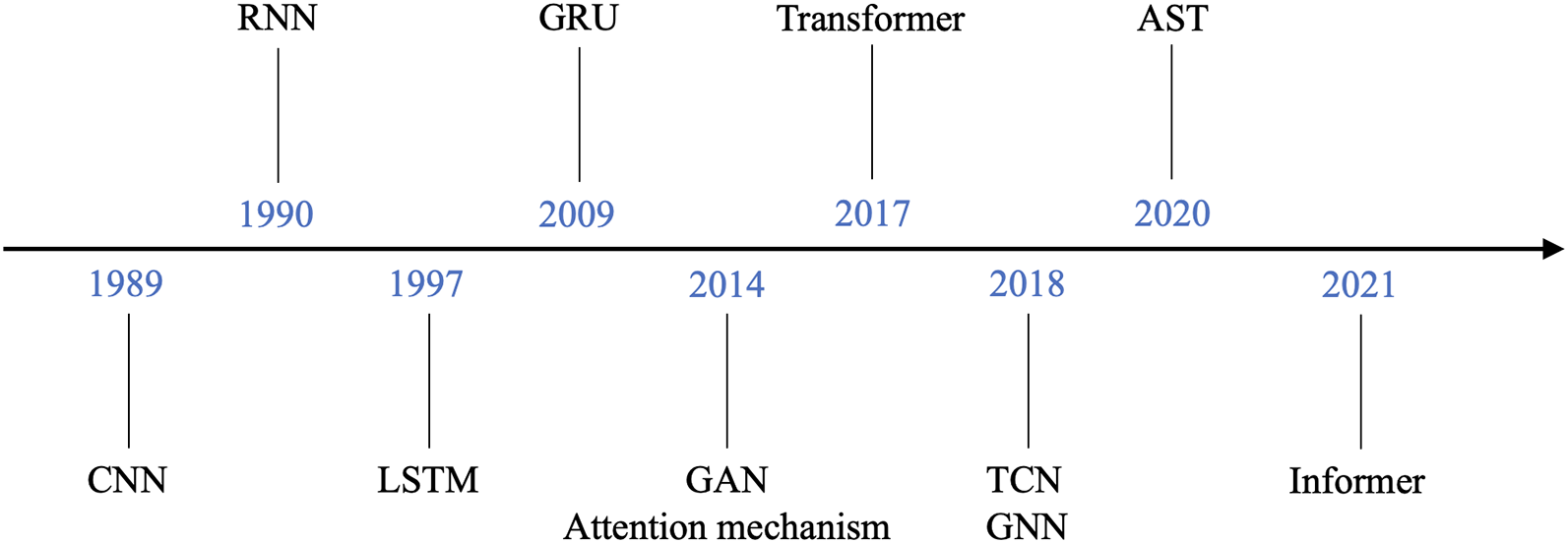
Figure 1: The development of DL-based TSF algorithms

Compared to other surveys [9,14,15], we offer a more comprehensive and accessible overview, integrating specific application scenarios and placing particular emphasis on recent advanced topics. The contributions of this paper are as follows:

•   Overview of Time Series Forecasting Tasks: We provide clear definitions of time series data and TSF, introducing and explaining the TSF task from various perspectives to enhance understanding.

•   New Classification and Comprehensive Review: We propose a new classification for TSF research, categorizing methods into CNN-based models, RNN-based models, GNN-based models, Transformer-based models, composite models, and other forecasting models. We summarize key issues in TSF and discuss relevant work and effective solutions for each.

•   Comprehensive Resources: We gather extensive resources, providing detailed introductions and reviews on various aspects of TSF, including definitions, commonly used models, and evaluation metrics. We also present the SOTA models from recent years, enabling scholars to gain a deeper understanding of TSF tasks and apply their knowledge in practice.

•   Future Research Directions: Based on our research and experimental findings, we outline potential future research directions, providing a forward-looking perspective on the field.

The remaining structure of the article is as follows: In Section 2, we define time series data and TSF, explaining the TSF task from various perspectives. In Section 3, we classify TSF methods according to different forecasting models and review state-of-the-art TSF methods [16]. In Section 4, we discuss and evaluate the datasets frequently used in TSF across various domains, along with their performance evaluation metrics. In Section 5, we speculate on the future trends of TSF research and briefly summarize the core findings of this study.

2  Problem Definition

In this section, we introduce the foundational concepts and definitions of the TSF problem. Specifically, we define data and its characteristics in Section 2.1, and discuss the definition of TSF and various approaches to the TSF task based on different classification criteria in Section 2.2.

2.1 Time Series Definition

Time series analysis serves as a fundamental methodology across diverse disciplines [16], ranging from quantitative finance and meteorological science to biomedical engineering and industrial applications. These temporally ordered observations record the evolution of system states, enabling researchers to identify underlying patterns, detect anomalies, and predict future behaviors. The analytical value of time series stems from their ability to represent dynamic processes through sequential measurements.

•   Trend: The trend component in time series analysis characterizes the persistent [16], long-term movement of data values, revealing either growth, decline, or stationary behavior across extended observation periods. This fundamental feature serves as a critical indicator of changes in the observed system, offering researchers meaningful information about the intrinsic dynamics of temporal processes.

For example, in equity market analysis, securities frequently demonstrate prolonged bullish trends during economic expansions, contrasted by bearish trends during contractions. These directional movements encapsulate the fundamental shifts in market valuation. As shown in Fig. 2, our analysis of product sales data reveals a consistent growth pattern, where the fitted trend line (dotted) clearly tracks the upward trajectory of actual sales measurements (solid line) over multiple business cycles.

Trends can manifest as either local or global patterns, and a single time series can exhibit both. For example, in the sales volume data, the overall trend is upward, but there may be localized upward trends during peak seasons and localized downward trends during off-seasons. Additionally, trends can be linear or non-linear [16]. A linear trend is characterized by a constant rate of increase or decrease, while a non-linear trend typically exhibits a multiplicative increase, meaning the rate of change is proportional to the previous values. Understanding the nature of the trend, whether it is linear or non-linear, is crucial for selecting appropriate forecasting models and strategies.

•   Seasonality: Seasonality in time-series data refers to the cyclical repeating patterns or periodic changes that occur over specific time frames. These cyclical variations are typically associated with particular seasons, months, days of the week, or other temporal units. For instance, in temperate regions, higher temperatures during the summer and lower temperatures during the winter create a distinct seasonal pattern. This pattern is crucial for weather forecasting and agricultural planning, among other applications. Similarly, stock markets are influenced by seasonality. The release of quarterly reports, annual reports, and financial data can significantly impact stock prices and trading volumes. Additionally, during specific seasons, such as the end of the year or the beginning of the year, investors may adjust their portfolios to accommodate seasonal changes. Fig. 3 illustrates the seasonal cycle of a product’s sales volume, highlighting the regular fluctuations that occur within a specific time frame.

•   Randomness: The randomness of a time series refers to the absence of a clear pattern, trend, or periodicity in the data over time. Instead, the data exhibit a high degree of variability and unpredictability, characterized by random fluctuations and irregularities. This randomness implies that the movements of the data are not governed by fixed patterns or laws, making it difficult to predict future values based solely on historical data. Randomness can be caused by a variety of factors, including external shocks, measurement errors, or inherent stochastic processes.

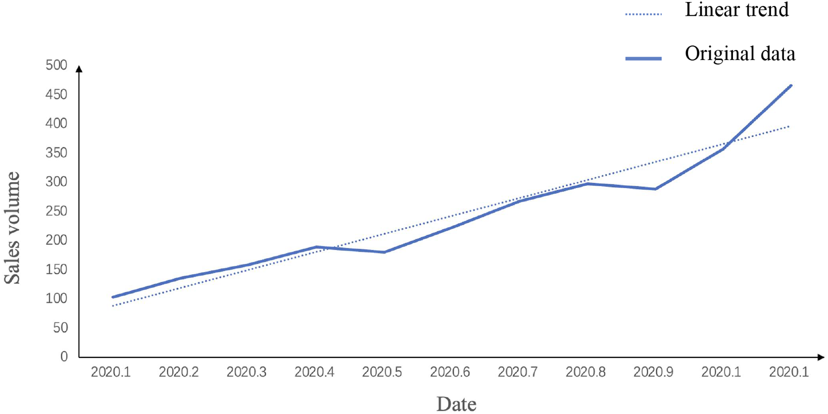
Figure 2: Trend in sales volume of a product

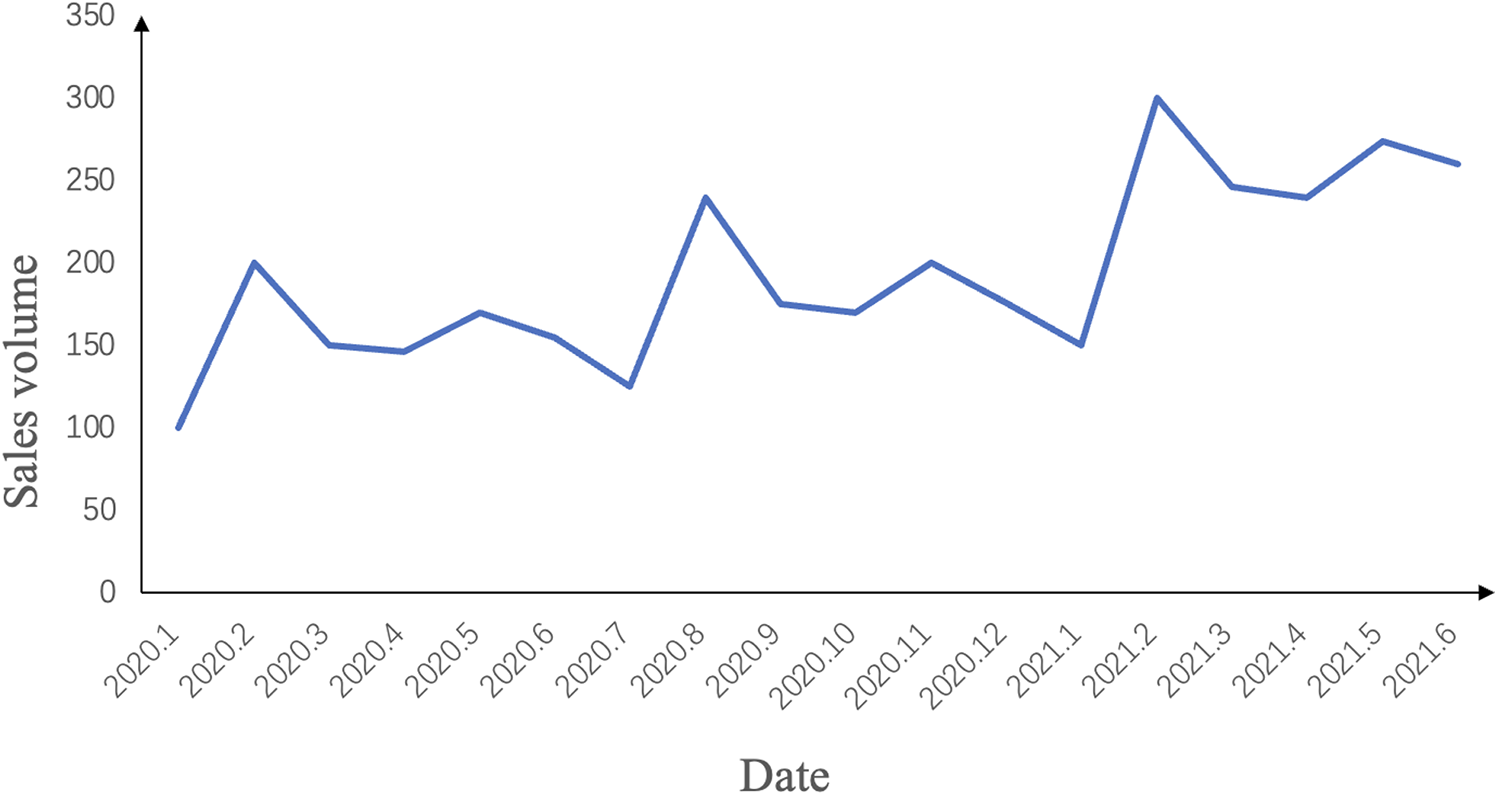
Figure 3: Seasonality in sales volume of a product

From a mathematical perspective, a time series is a sequence of random variables, either finite or infinite, arranged in chronological order. These variables represent the values of a specific statistical indicator over time, typically sampled at a relatively fixed frequency to capture the process of change. Mathematically, a time series can be conceptualized as a stochastic process, where each observation is a random variable influenced by various factors.

The time series data can be represented in matrix form as follows. When there is only one sensor, the time series is one-dimensional:

X^t={x→1,x→2,…,x→t}(1)

where x→t represents the value of the sensor at the current timestamp, and X^t represents a set of time series. This can be extended to multidimensional time series:

X^1:N,t−n:t={x→1,t−n:t,x→2,t−n:t,…,x→N,t−n:t}(2)

where N denotes an N-dimensional time series, n represents a time series with n sample data, and t denotes the current time step. x→1,t−k:t denotes a vector, x→1,t−n:t={x1,t−n,x1,t−n+1,…,x1,t}, and x1,t denotes the time series point of the time series at time t. X^1:N,t−n:t denotes N-dimensional time series data consisting of N time series.

Time series data can be either one-dimensional or multidimensional. A one-dimensional time series, focusing on a single variable, is represented as:

X^t−k,t={x1,t−k,x1,t−k+1,…,x1,t}(3)

where X^t−k,t represents the time series of the past k time series. This representation is particularly useful for analyzing the behavior of a single variable over time, such as the daily closing price of a stock or the hourly temperature readings at a specific location. Understanding the mathematical structure of time series data is fundamental for developing effective models and techniques for time series forecasting.

2.2 Definition of Time Series Forecasting

TSF serves as a fundamental analytical technique for temporal data analysis, with wide-ranging applications including classification tasks, anomaly identification, and future value prediction. At its core, TSF methodologies employ historical observations to model temporal patterns, enabling the projection of future system states through careful analysis of established trends and behavioral characteristics. The primary objective involves generating accurate predictions for time steps beyond a given reference point t, utilizing only information available prior to t.

For clarity of exposition, we focus our discussion on single-step forecasting scenarios. The underlying mathematical formulation can be expressed as:

X^i,t+1=f(Xi,t−k:t,S)(4)

where i denotes the i-th set of time series data, X^i,t+1 represents the forecasted value at time t+1 based on the data from t−k to t, S represents the static factors that remain constant during the forecasting process, and f(⋅) is the prediction function of the model. Since the static factor S remains unchanged during the forecasting process, in order to simplify the formulas for better understanding, S will be omitted in the subsequent equations.

TSF methodologies can be classified according to two primary dimensions: (1) prediction horizon, encompassing single-step (immediate next point) and multi-step (extended future sequence) forecasting approaches, and (2) input variable configuration, distinguishing between autoregressive (target series only) and covariate-based (incorporating external factors) methods. This categorization reflects fundamental differences in problem formulation and technical requirements, with each paradigm presenting unique computational challenges and application scenarios that will be explored in subsequent sections.

2.2.1 Single-Step Forecasting and Multi-Step Forecasting

TSF methodologies can be fundamentally classified by their prediction horizon, with single-step forecasting (one-step-ahead prediction) focusing on immediate future values and multi-step forecasting (also called long-horizon prediction) addressing sequences of future observations. Each type of forecasting serves different purposes and is suited to different scenarios.

(1) Single-Step Forecasting

Single-step forecasting focuses on estimating the immediate subsequent value in a time series using historical observations (Fig. 4). This methodology is particularly valuable in applications requiring high temporal resolution, including financial market analysis and meteorological prediction systems, where accurate near-term projections are essential for operational decision-making. The technique’s emphasis on the most proximate future point enables enhanced prediction accuracy for real-time applications, as it avoids the compounding errors associated with longer forecasting horizons while providing the low-latency outputs needed for time-sensitive scenarios.

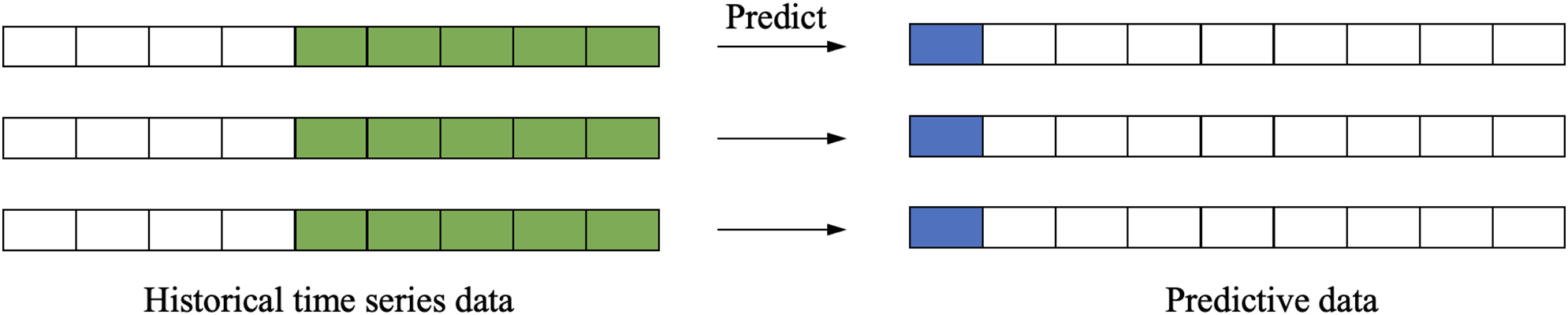
Figure 4: Single-step forecasting

The mathematical expression for single-step forecasting is as follows:

X^j,t+1=f(Xi,t−k:t,S)(5)

where i denotes the number of input features, j is the number of output features, k is the time step parameter [9], and t is the current time step, S denotes any static factors that remain constant during the forecasting process.

(2) Multi-Step Forecasting

Multi-step forecasting extends predictive capabilities by generating sequential future values from historical observations (Fig. 5), addressing scenarios requiring extended-horizon projections. This methodology is indispensable for applications where capturing evolving trends is critical, such as electricity load planning, macroeconomic policy formulation, and investment portfolio optimization. By simultaneously modeling multiple future states, it enables proactive resource allocation and risk mitigation, though it introduces unique challenges like error accumulation and temporal dependency decay that require specialized architectural solutions.

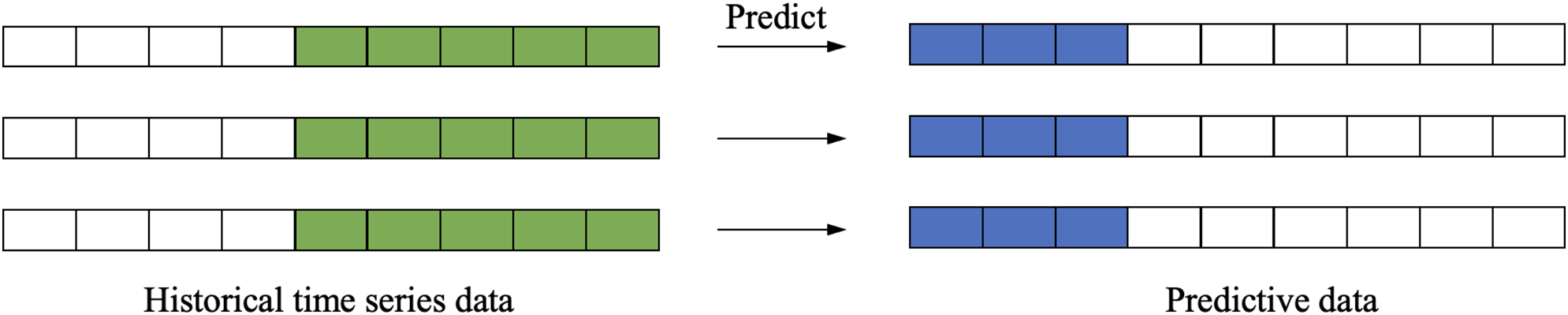
Figure 5: Multi-step forecasting

The mathematical expression for multi-step forecasting is as follows:

X^j,t+1:t+s+1=f(Xi,t−k:t,S)(6)

where s denotes the prediction horizon, representing the number of future time steps to be predicted, X^j,t+1:t+s+1 represents the predicted values for the j-th output feature from time t+1 to t+s+1.

Multi-step forecasting can be implemented using several methods, each with its own advantages and disadvantages. The four main methods are:

1.    Direct Multi-Step Forecasting: This method involves building a separate model for each future time step. Each model is trained to predict a specific time step, and the predictions are aggregated to form the final forecast. While this approach can capture the unique patterns of each time step, it can become computationally intensive when the prediction horizon is large, as it requires training multiple models.

2.    Recursive Multi-Step Forecasting: In this method, a single model is used to predict the next time step, and the predicted value is then fed back into the model as an input for the subsequent prediction. This process is repeated recursively to generate predictions for multiple future time steps. While this approach is computationally efficient, it can accumulate errors over time, leading to less accurate long-term predictions.

3.    Direct-Recursive Hybrid Multi-Step Forecasting: This method combines the direct and recursive approaches. It uses a separate model for each time step but also incorporates the predictions from previous time steps as inputs [10]. This hybrid approach aims to balance the computational efficiency of the recursive method with the accuracy of the direct method.

4.    Multi-Output Forecasting: This method involves training a single model to predict all future time steps simultaneously. The model is designed to handle multiple outputs, capturing the relationships between different time steps. This approach can be more efficient and accurate, especially when the relationships between time steps are strong.

These methodologies exhibit distinct advantages and limitations, with optimal model selection contingent upon both dataset properties (e.g., temporal resolution, noise characteristics) and application requirements (e.g., prediction horizon, interpretability needs).

Direct Multi-Step Forecasting. To build a separate model for each future time step, direct multi-step forecasting involves training each model to predict a specific time step. Essentially, this method is a series of single-step forecasts, with each model trained on the same historical data but predicting a different future time step, as shown in Fig. 6. The mathematical expression for direct multi-step forecasting is as follows.

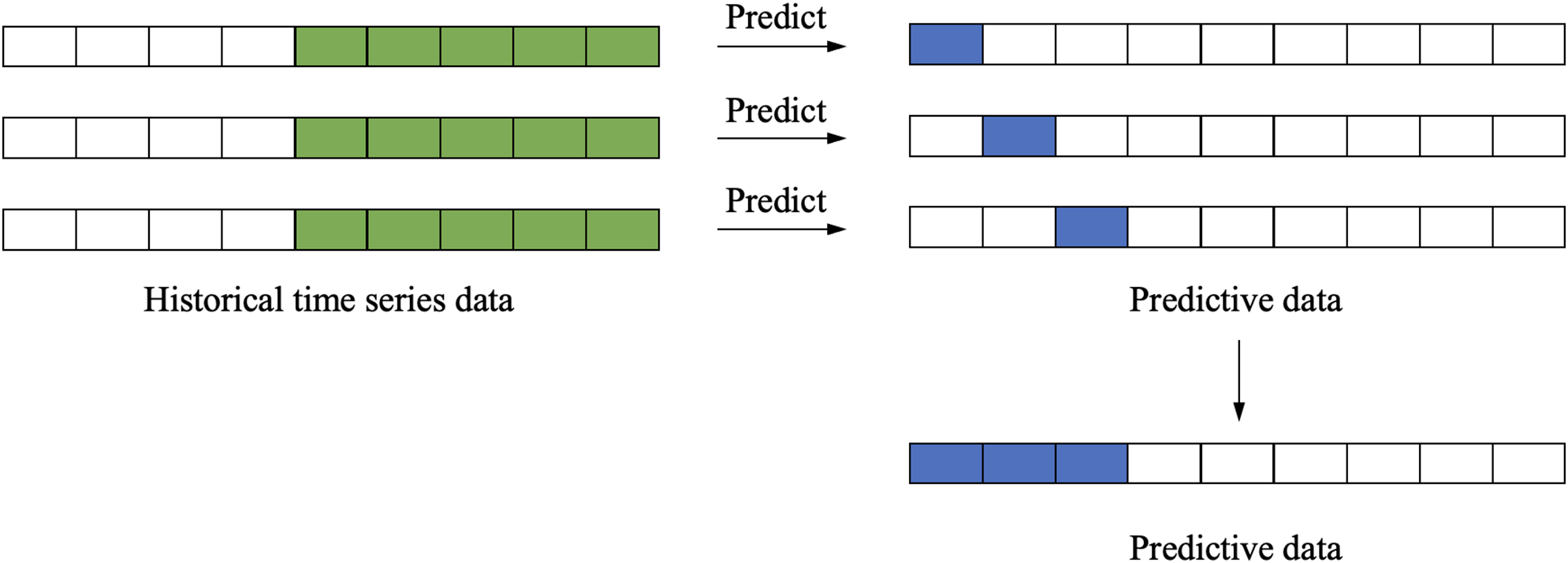
Figure 6: Direct multi-step forecasting

The mathematical expression for direct multi-step prediction is as follows:

X^i,t+1=f1(Xi,t−k:t)X^i,t+2=f2(Xi,t−k:t)…X^i,t+s+1=fs+1(Xi,t−k:t)(7)

where i denotes the number of input features, k denotes the time step and t denotes the current time step, and s denotes the predicted horizon.

While direct multi-step forecasting can capture the unique patterns of each time step, it can become computationally intensive when the prediction horizon is large, as it requires training multiple models. Additionally, since each model is trained independently, it may not capture the correlations between different time steps, potentially leading to less accurate predictions.

Recursive Multi-Step Forecasting. It employs an iterative prediction strategy where a single-step model generates successive forecasts by recursively feeding its outputs as inputs for subsequent time steps (Fig. 7). This chained prediction mechanism can be formalized as:

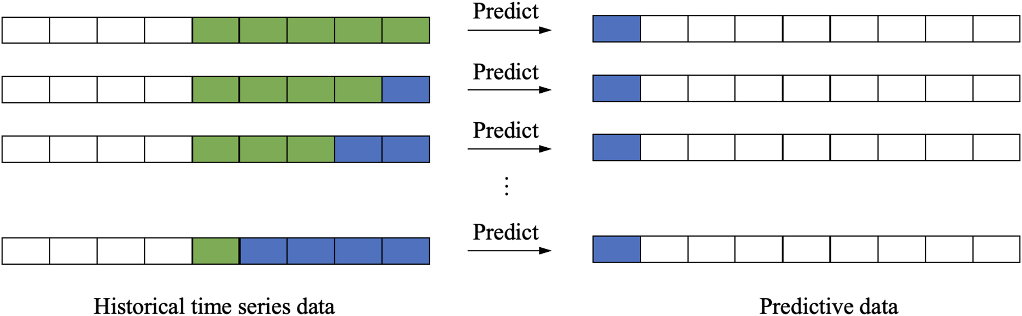
Figure 7: Recursive multi-step forecasting

The mathematical expression is as follows:

X^i,t+1=f(Xi,t−k:t)X^i,t+2=f(X^i,t+1)…X^i,t+s+1=f(X^i,t+2)(8)

where i denotes the number of input features, k denotes the time step and t denotes the current time step, and s denotes the predicted horizon [9].

While recursive multi-step forecasting is computationally efficient, it can accumulate errors over time, leading to less accurate long-term predictions. This is because the model uses predicted values rather than actual observations as inputs for subsequent predictions.

Direct-Recursive Hybrid Multi-Step Forecasting.It approach enhances multi-step forecasting accuracy by synergistically integrating the strengths of both direct and recursive methodologies. This framework employs a cascade of specialized models, where each subsequent predictor incorporates outputs from preceding models as supplementary inputs (Fig. 8). The mathematical formulation of this hybrid paradigm can be expressed as:

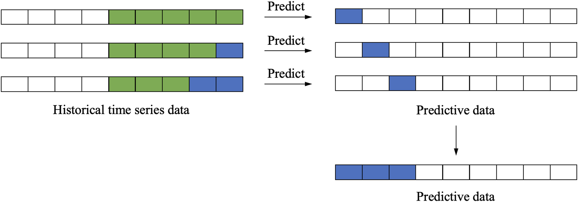
Figure 8: Direct-recursive hybrid multi-step forecasting

The mathematical expression for direct-recursive hybrid multi-step prediction [10] is as follows:

X^i,t+1=f1(Xi,t−k:t)X^i,t+2=f2(Xi,t−k+1:t+1)…X^i,t+s+1=fs+1(Xi,t−k+s:t+s)(9)

where i denotes the number of input features, k denotes the time step and t denotes the current time step, and s denotes the predicted horizon.

This hybrid approach aims to balance the computational efficiency of the recursive method with the accuracy of the direct method by leveraging the strengths of both approaches.

Multi-Output Multi-Step Forecasting. Training a single model to predict all future time steps simultaneously, multi-output multi-step forecasting is particularly useful in neural network models can handle multidimensional inputs and outputs. Computationally efficient, this method captures the relationships between different time steps, making it a powerful tool for long-term forecasting.

2.2.2 Autoregressive Forecasting and Covariate Forecasting

TSF methodologies can be fundamentally classified by their input variable structure into two paradigms: (1) autoregressive approaches that exclusively utilize historical values of the target series, and (2) covariate-based methods that incorporate external explanatory variables. The selection between these approaches requires careful consideration of multiple factors, including data dimensionality, feature availability, and the required prediction horizon, as each technique exhibits distinct advantages in handling different temporal patterns and application scenarios.

(1) Autoregressive forecasting

Autoregressive forecasting involves using only the time series data itself for prediction, without considering other external factors, as illustrated in Fig. 9. By leveraging historical data, an autoregressive model can be built to predict future values. These models typically use linear regression methods to fit the historical data and make predictions based on the fitting results.

Figure 9: Autoregressive forecasting

The advantages of autoregressive forecasting include its simplicity, ease of use, and computational efficiency. However, it has some limitations. It can capture linear relationships and is well-suited for handling nonlinear data. Additionally, it cannot effectively model seasonal or trend components. Therefore, when using autoregressive forecasting, it is important to select appropriate models and parameters based on the specific characteristics of the data. Autoregressive forecasting is typically used for short-term predictions, as it focuses solely on the patterns within the time series data and does not account for external influences.

The mathematical expression for autoregressive prediction is as follows:

X^t+1=f(Xt−k:t)(10)

where t denotes the current time step and k denotes the input time step size [9]. f represents the algorithm of the model in the current application scenario.

(2) Covariate forecasting

Covariate forecasting extends the forecasting model by incorporating additional external factors, or covariates, in addition to the time series data itself, as shown in Fig. 10. These covariates can include variables. By modeling the relationships between these covariates and the target variable, covariate forecasting can provide more accurate and comprehensive predictions.

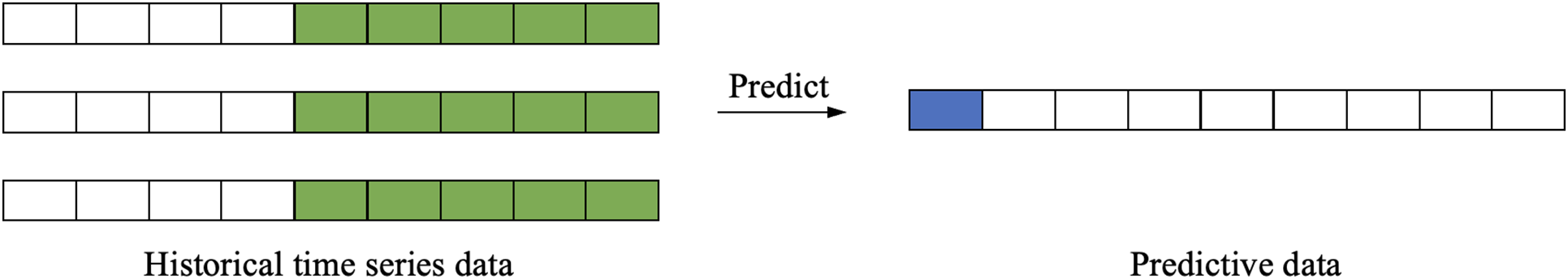
Figure 10: Covariate forecasting

The primary advantage of covariate forecasting is its ability to improve prediction accuracy by considering a broader range of relevant factors. For example, in sales forecasting, covariates such as weather, economic indices, and promotional activities can be included to enhance the predictive power of the model. It requires the collection and processing of additional data, which can increase the complexity and computational cost. Moreover, selecting the appropriate covariates is crucial and often requires domain expertise and careful analysis.

The mathematical expression for covariate prediction is given below:

X^1,t+1=f(Xi,t−k:t)(11)

where i indicates the number of input features, k means the input time step size [9], and t refers to the current time step.

In summary, autoregressive forecasting is a simple and efficient method suitable for short-term predictions when the focus is on the inherent patterns of the time series data. Covariate forecasting, on the other hand, is more complex but can provide higher accuracy by incorporating external factors that influence the target variable.

2.2.3 Isometric Interval Forecasting and Non-Isometric Interval Forecasting

Time series forecasting (TSF) tasks can also be classified based on the equality of the time intervals between observations in the time series data. The two main categories are isometric interval forecasting and non-isometric interval forecasting, which are described below.

(1) Isometric Interval Forecasting

Isometric interval forecasting involves predicting future values based on time series data where the time interval between each observation is equal, as illustrated in Fig. 11. This method is particularly suitable for data that exhibit periodic patterns. When the data have significant periodic variations, isometric interval forecasting can effectively capture these patterns and use them to predict future values.

Figure 11: Isometric interval forecasting

The primary advantage of isometric interval forecasting is its ability to capture and utilize periodic patterns in the data. For instance, in the field of finance, stock prices often exhibit cyclical behavior, and isometric interval forecasting can be effectively used to predict future stock prices. Similarly, in meteorology, temperature and rainfall data often show cyclical variations, making isometric interval forecasting a suitable method for predicting future weather conditions.

The mathematical expression for isometric interval forecasting is as follows:

X^t+1=f(Xi,t−k,Xi,t−k+1,Xi,t−k+2,…,Xi,t)=f(Xt−k:t)(12)

where i is the i-th time series data, t denotes the current time step, and k is the input time step size.

(2) Non-Isometric Interval Forecasting

Non-isometric interval forecasting deals with time series data where the time interval between observations is unequal, as shown in Fig. 12. This method is suitable for data that do not exhibit a clear periodic pattern. Non-isometric interval forecasting can be used to make predictions even when there is no apparent periodic variation in the data. For example, in the finance domain, stock trading data may be non-equally spaced.

Figure 12: Nonisometric interval forecasting

The advantage of non-isometric interval forecasting is its ability to handle non-equally spaced data and make predictions even in the absence of significant cyclical variations. However, this method has some limitations. First, it requires more complex techniques, such as interpolation, to handle the unequal intervals, which can increase computational complexity and resource requirements. Additionally, non-isometric interval forecasting may be less accurate than isometric interval forecasting because it cannot utilize periodic patterns in the data for prediction.

The mathematical expression for non-isometric interval forecasting is as follows:

X^t+1=f(Xi,t−k,Xi,t−k+l1,Xi,t−k+l2,…,Xi,t)=f(Xt−k:t)(13)

where i denotes the i-th time series data, t represents the current time step, k is the input time step size, and {l≤k|l1,l2,l3,…,ln∈N+}. Equalities may exist between some values of l, but not all values before l are identical, as there are varying sizes of l.

In summary, isometric interval forecasting is suitable for data with regular and periodic patterns, while non-isometric interval forecasting is used for data with irregular or non-periodic patterns.

3  A Review and Classification of DL Techniques in TSF

In this section, we present and discuss typical time series forecasting (TSF) approaches based on different deep learning models. We categorize TSF methods into five types: CNN-based methods, RNN-based methods, MLP-based methods, GNN-based methods, and Transformer-based methods. For each category, we explain the principles and roles of the methods in addressing TSF problems and provide a review of specific methods.

•   CNN-Based Methods: Convolutional Neural Networks are designed to extract local features from time series data through convolutional layers. This method is particularly effective for capturing short-term dependencies in the data, making it suitable for tasks like financial prediction, where local patterns in price movements are important.

•   RNN-Based Methods: Recurrent Neural Network is ideal for time series forecasting, because they can model temporal dependencies by maintaining a memory of past inputs.

•   MLP-Based Methods: Multi-Layer Perceptrons are feedforward neural networks that can model both linear and nonlinear relationships in time series data. They are useful for forecasting tasks like sales prediction, where multiple input features, such as seasonality or promotional events, need to be combined to predict future outcomes.

•   GNN-Based Methods: Graph Neural Network is designed to handle time series data with complex spatial-temporal dependencies. They are especially useful for tasks like traffic flow prediction.

•   Transformer-Based Methods: Transformer models use self-attention mechanisms to handle long-term dependencies in time series data. Unlike RNNs, transformers can process sequences in parallel and efficiently model long-range dependencies.

Shallow networks are typically suitable for handling simple forecasting problems, with the advantage of lower computational cost and faster training speed. However, as the complexity of the problem increases, shallow networks may fail to capture the deeper relationships and patterns in the data. In such cases, deep networks become more necessary. Although deep networks have significantly higher computational costs than shallow networks, they can effectively learn more complex feature representations, especially when dealing with nonlinear, high-dimensional, or long-term dependent data. By introducing more layers, deep networks can capture more detailed patterns, and in many practical problems, deep networks have been shown to significantly improve forecasting accuracy.

The training and inference processes of DL models typically require substantial computational resources, especially when handling large datasets. The costs during training mainly stem from the model’s complexity, the number of parameters, and the iterative processing of data. DLg models often require large memory and processing power. While inference is relatively lighter, highly complex models still consume significant time, particularly during real-time or large batch predictions. Additionally, using hardware accelerators like GPUs or TPUs during training incurs high energy consumption and operational costs. For simple problems, shallow networks remain an efficient choice, while for complex problems, deep networks offer stronger modeling capabilities. We not only conduct a detailed analysis and explanation of the models but also provide a side-by-side performance summary. We implement the model with the PyTorch toolkit on a Linux server with a GeForce RTX 4090 GPU.

3.1 CNN-Based Methods

The structure of the Convolutional Neural Networks (CNNs) used for TSF is shown in Fig. 13. For ease of understanding, a single-channel solution, as shown in Eq. (3), is used.

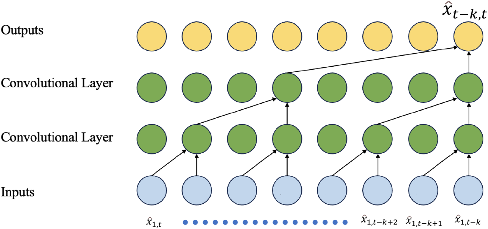
Figure 13: The structure of the CNN used for the TSF task

The working principle of CNNs is based on convolutional operations and feature extraction. In TSF tasks, CNNs can capture patterns and local dependencies at different time scales and extract the most predictive features from time series data. Additionally, CNNs can handle multivariate time series data by using 2D CNNs, which can extract important feature patterns in both time and other dimensions simultaneously.

Temporal Convolutional Networks (TCNs) [17] are an improvement over traditional CNNs. TCNs use convolutional layers to capture patterns and dependencies in time series data and have shown strong performance in various time series tasks. The key improvements in TCNs include three blocks, as shown in Figs. 14–16.

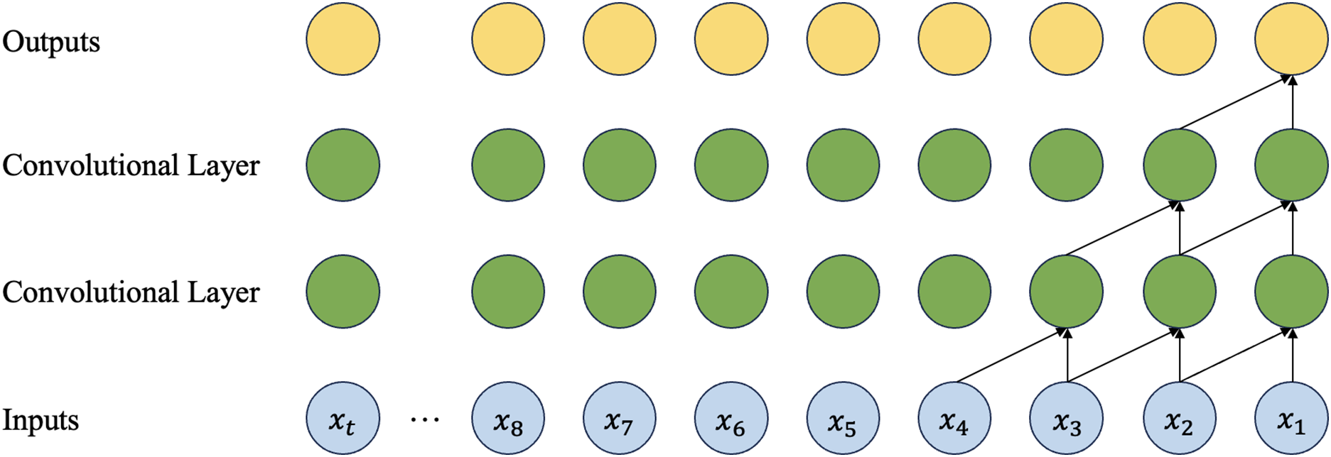
Figure 14: The structure of the causal convolution in TCN

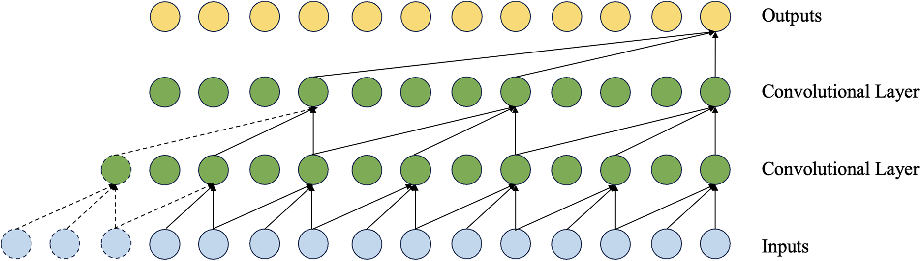
Figure 15: The structure of the dilated convolution in TCN

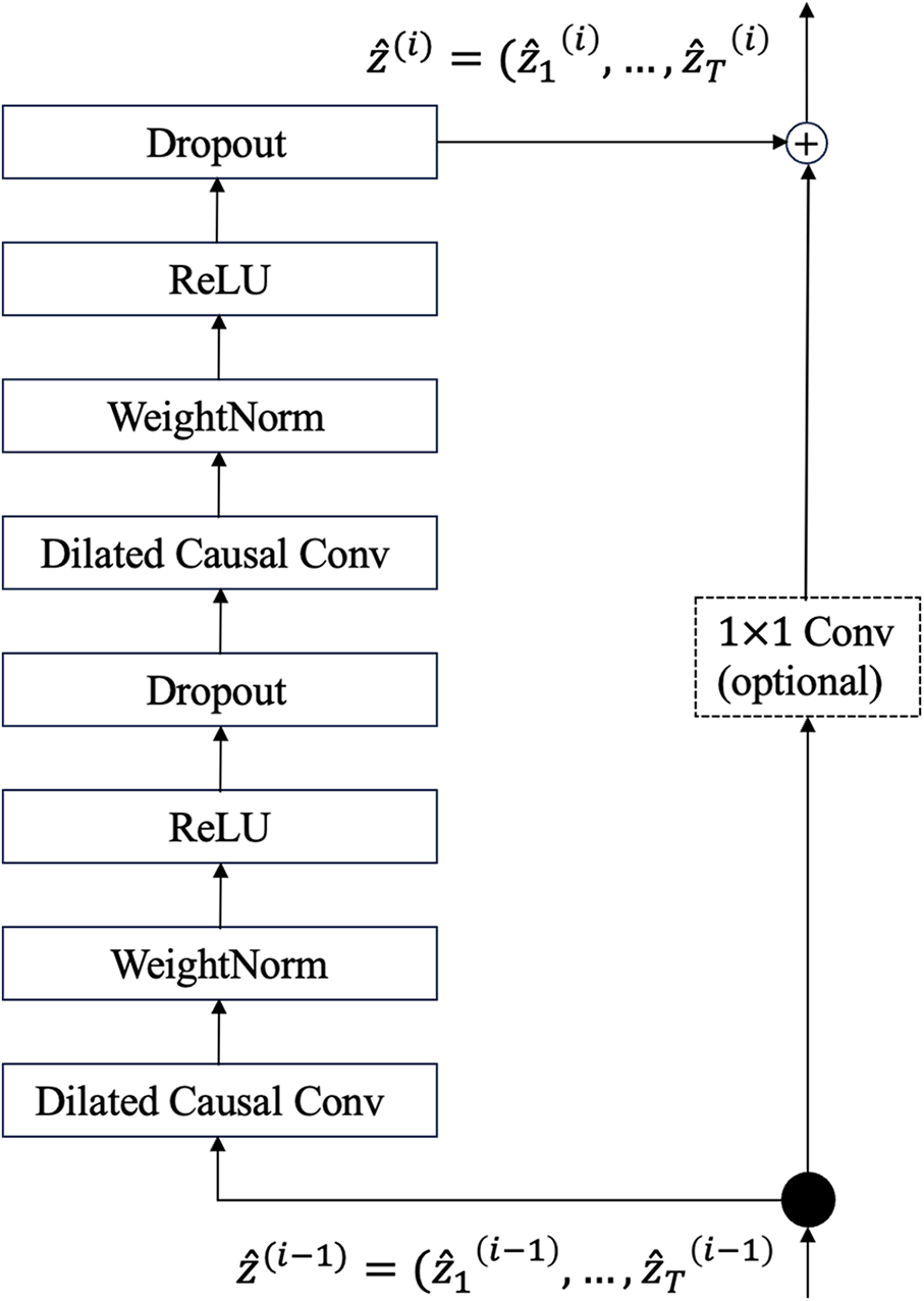
Figure 16: The structure of the residual block in TCN

•   Causal Convolution: In causal convolution, the convolution kernel only slides over current and past time steps, ensuring that the model uses only past information to predict the current output, following a causal relationship.

•   Dilated Convolution: Dilated convolution architectures enhance temporal dependency modeling through strategically spaced convolutional kernels, expanding the receptive field while maintaining parameter efficiency.

•   Residual Blocks: Residual blocks use residual connections to solve the problem of vanishing gradients in deep networks. They allow gradients to flow directly to earlier layers, improving network performance and supporting the construction of deeper networks.

As shown in Fig. 15, dilated convolution in Temporal Convolutional Networks is a technique that expands the receptive field by introducing gaps between the data points the kernel processes. This is done by applying a kernel with a specified “dilation rate,” allowing the model to capture long-range dependencies without increasing the computational load. By stacking dilated convolutions with increasing dilation rates, TCNs can model dependencies at various time scales. In the network at each update step, dropout forces the network to rely on multiple paths to make predictions. This helps to reduce the model’s dependency on specific neurons, thereby improving generalization to unseen data. Dropout is typically applied in fully connected layers and can be controlled, which specifies the probability of deactivating a neuron. By introducing dropout, the network is encouraged to learn more robust features, especially in complex tasks with limited training data.

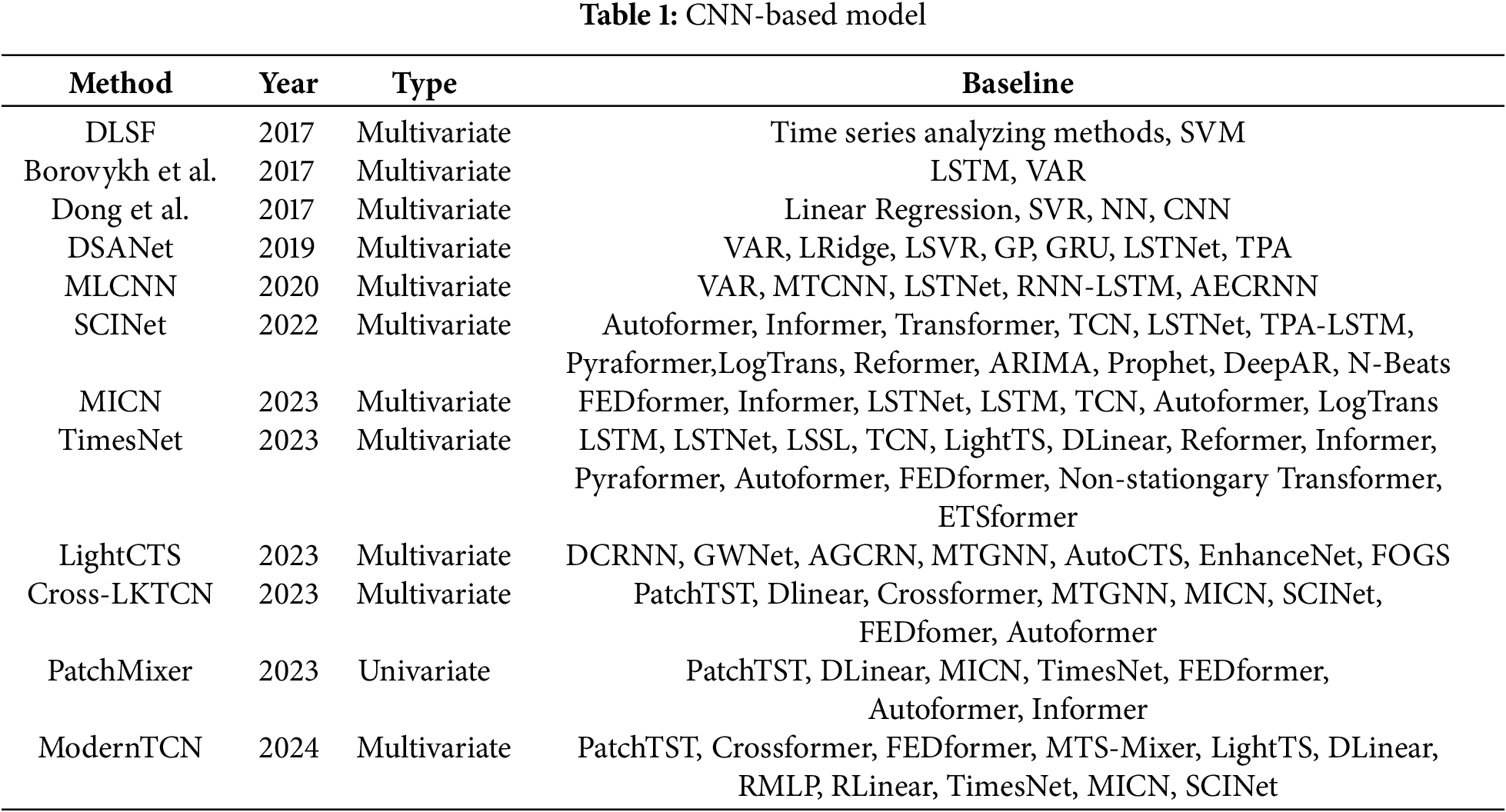
Some TSF works based on CNN and TCN modeling are discussed below, as shown in Table 1.

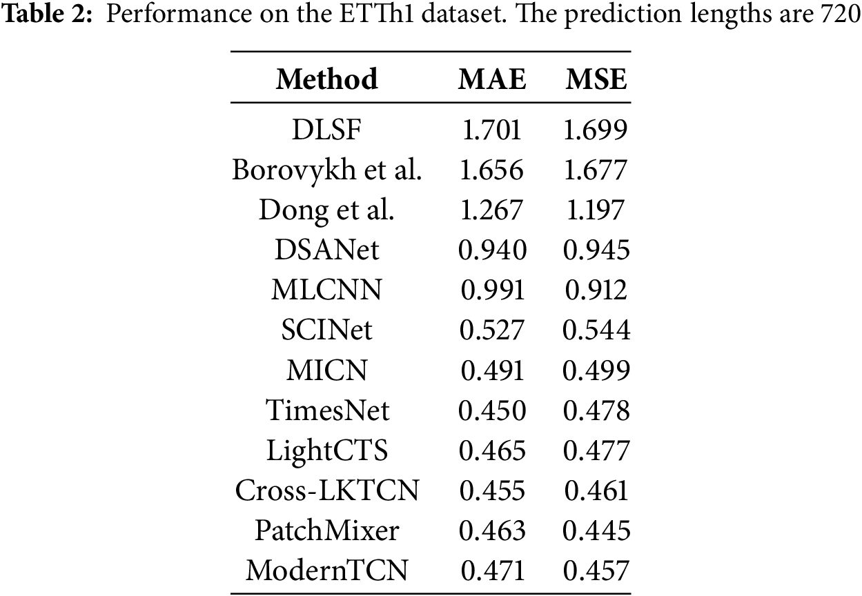
As shown in Table 2, we evaluate the overall performance of the model on the ETTh1 dataset with a prediction length of 720.

Li et al. [18] proposed a deep learning-based prediction method, DLSF, which converts time series data into images for processing. For feature extraction, they designed a two-branch convolutional neural network. Finally, a linear autoregressive component is integrated to enhance robustness, making it suitable for dynamic cyclic or non-cyclic sequence prediction. For data prediction, they proposed a multilayer neural network to predict data changes. This method is used for power load prediction and takes into account external influences. The results showed good accuracy and efficiency on a load dataset from a major city in China. Borovykh et al. [19] proposed a CNN model for financial predictive analytics inspired by the deep convolutional WaveNet architectural model. The model uses the ReLU activation function and employs parametric skip-connection conditioning to simplify and optimize the structure of the TSF forecasting model.

Although CNN performs well in prediction on some small-scale datasets, as the datasets become larger and more complex, CNN may appear to perform poorly on large datasets. To address this issue, Dong et al. [20] proposed a model that combines CNN with the K-means clustering algorithm to achieve better accuracy and scalability. This method divides the dataset into different smaller sub-datasets using K-means and trains the CNN on the generated sub-datasets. The performance of the method on a large power dataset with more than 10,000 samples proves its effectiveness and high performance.

Current time series forecasting approaches predominantly focus on single-point prediction, failing to account for temporal interdependencies between forecasts at varying horizons, which consequently constrains their predictive performance. To bridge this gap, Cheng et al. [21] introduced the Multi-Level Conformational Neural Network (MLCNN), an innovative multi-task learning architecture inspired by human predictive cognition. MLCNN uniquely integrates: (1) shared feature extraction across temporal scales, (2) dynamic fusion of multi-horizon predictive mechanisms, and (3) explicit modeling of cross-horizon interaction patterns—collectively enhancing forecast accuracy through synergistic temporal relationship learning.

Generic models used to solve the TSF problem do not take into account the specificity between time series data well. To solve this problem, Liu et al. [22] proposed Sample Convolution and Interaction Network (SCINet) to address the issue of generic models not accounting for the specificity between time series data. SCINet uses a downsampled convolutional interaction framework to simulate complex dynamic time series for better prediction. The SCI-Block module in this network structure extracts the input time series data and its features into two subsequences through downsampling, allowing the network to better learn the complex and rich features of the input time series.

To address the dual challenges of computational complexity in Transformer architectures and their limited capacity for local feature extraction, Wang et al. [23] developed the Multi-scale Isometric Convolution Network (MICN). This innovative framework integrates parallel convolutional branches to simultaneously capture: (i) fine-grained local patterns through isometric kernels, and (ii) global temporal dependencies via hierarchical feature fusion. The multi-scale design explicitly decouples short-range and long-range modeling, achieving superior efficiency while maintaining modeling fidelity compared to conventional attention-based approaches.

To enhance the modeling capacity for complex temporal patterns, Wu et al. [24] introduced TimesNet, an innovative framework that transforms 1D time series into multiple 2D tensors through periodic decomposition. This novel representation: (i) encodes intra-cycle variations along tensor columns, (ii) captures inter-cycle dynamics through tensor rows, and (iii) enables efficient 2D convolution operations for joint temporal pattern learning. The architecture demonstrates state-of-the-art performance across five benchmark time series analysis tasks by effectively leveraging both microscopic periodic fluctuations and macroscopic trend evolution through its unique 2D transformation paradigm.

To mitigate the computational inefficiency of existing deep learning models for correlated time series forecasting without sacrificing accuracy, Lai et al. [25] developed LightCTS—a lightweight framework employing streamlined temporal-spatial operator stacking. Unlike conventional architectures with alternating layers, LightCTS adopts: (i) parallelized operator modules for reduced computational overhead, (ii) optimized feature interaction mechanisms through simplified tensor operations, and (iii) adaptive weight sharing across prediction horizons.

Luo and Wang [26] proposed a convolution-based network architecture, CrossLKTCN, which addresses the problem that existing methods mainly focus on cross-temporal dependencies and do not adequately consider cross-variate dependencies. Gong et al. [27] proposed a novel CNN-based model, PatchMixer, to address the problem of temporal information loss due to the alignment-agnostic mechanism of transformer-based methods. PatchMixer retains temporal information by using a variational convolutional structure, relying solely on depth-separable convolution and using a single-scale architecture to simultaneously extract local features and global correlations of temporal information. Luo and Wang [28] brought the CNN convolutional model back into the spotlight by adapting the traditional Temporal Convolutional Network (TCN) and modifying it into a more suitable model for time series tasks, namely ModernTCN. ModernTCN adopts a large convolutional kernel, enhancing the receptive field. The method also leverages the ability of convolution to capture dependencies between variables, using three sets of convolutions to cleverly realize the decoupling modeling of three relationships: temporal, channel, and variable.

In summary, they may perform less effectively in modeling global patterns and complex time-series structures, such as non-smoothness, seasonality, or periodicity.

3.2 RNN-Based Methods

Recurrent Neural Networks (RNNs), first proposed by Elman [29], play a crucial role in time series forecasting (TSF) tasks. RNNs are characterized by their recurrent connectivity, which allows them to store past information and utilize it in the current time step by introducing recurrent dependencies on the temporal dimensions. The structure of the RNN is shown in Fig. 17.

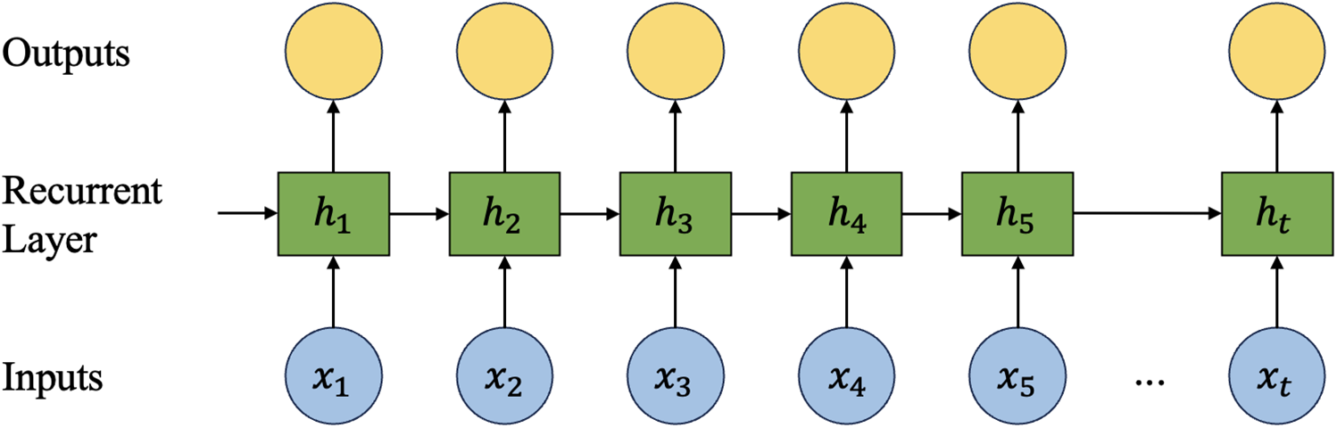
Figure 17: The structure of the RNN used for the TSF task

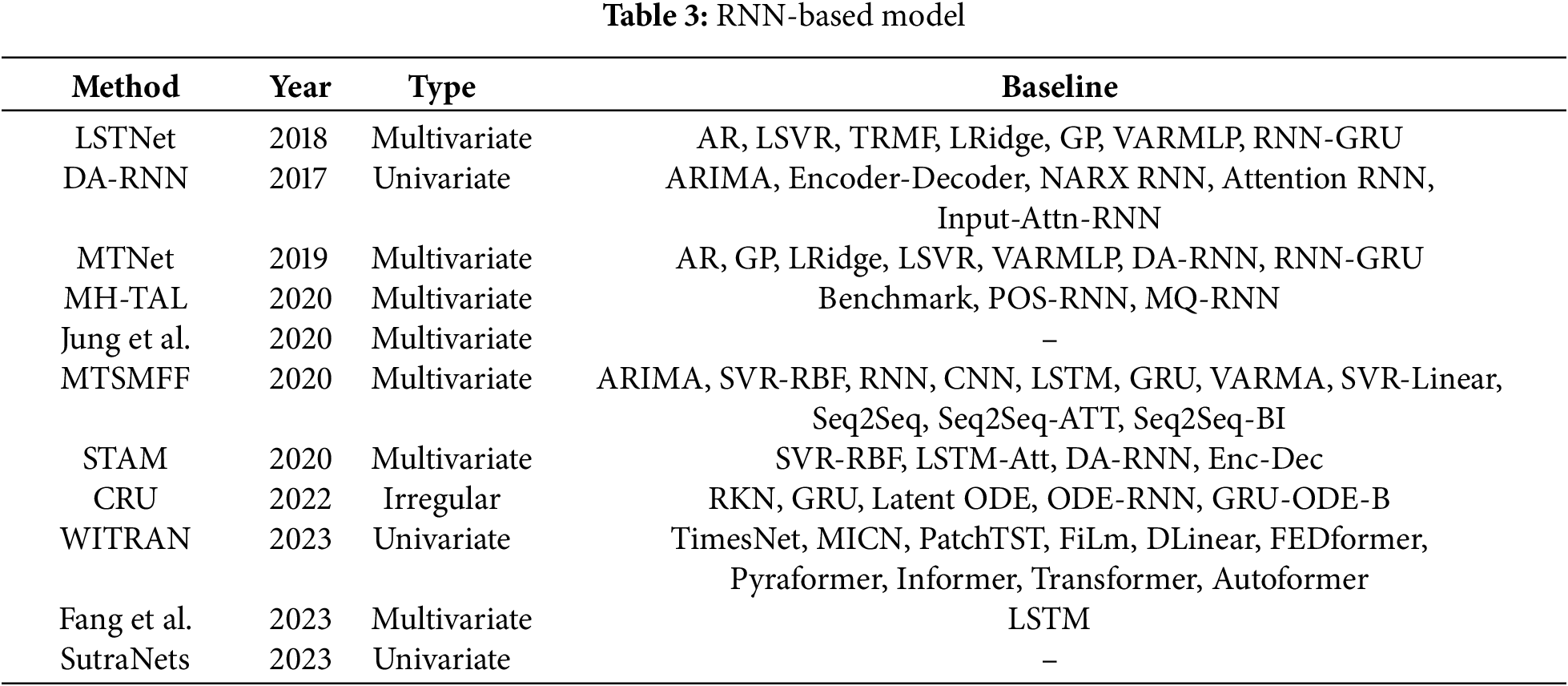
Despite the suitability of RNNs for processing time series information, they have limitations in handling long sequences of temporal data and suffer from the vanishing gradient problem. To address these issues, Graves [30] introduced Long Short-Term Memory (LSTM). LSTM efficiently captures and conveys long-term dependencies in time series by incorporating memory units and gating mechanisms, thereby avoiding the gradient vanishing problem inherent in RNNs. Although LSTM solves the issues of RNNs, its complex structure demands greater computational resources and results in slower network training. To simplify the model, Cho et al. [31] proposed the Gated Recurrent Unit (GRU) as a streamlined version of LSTM. GRU contains only two gating mechanisms: the update gate and the reset gate. The update gate controls the weights of past memories and current inputs, while the reset gate determines the impact of past memories on current inputs. Some TSF methods based on RNN models are described below, as shown in Table 3.

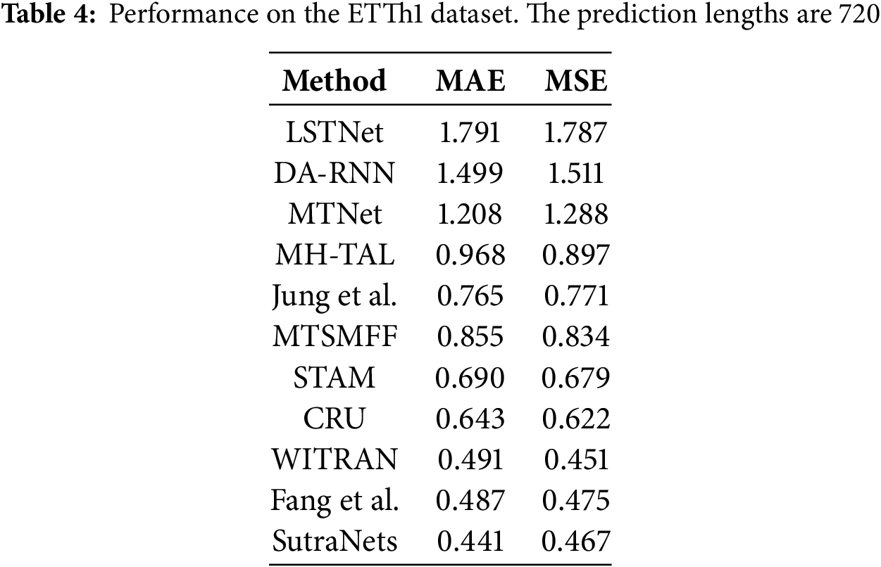
As shown in Table 4, we evaluate the overall performance of the model on the ETTh1 dataset with a prediction length of 720.

Lai et al. [32] developed the Long- and Short-term Time Series Network (LSTNet), which synergistically combines convolutional layers for local pattern extraction with recurrent units for trend modeling, demonstrating superior performance on real-world datasets exhibiting complex periodic behaviors. Complementing this approach, Qin et al. [33] proposed the Dual-Stage Attention-Based RNN (DARNN), incorporating: (i) an input attention mechanism for dynamic feature selection based on historical encoder states, and (ii) a temporal attention module specifically designed to model extended dependencies.

Recent innovations in temporal modeling have introduced memory-enhanced architectures to overcome limitations in capturing complex temporal dependencies. Chang et al. [34] developed the Memory Time-series Network (MTNet), incorporating: (i) a large memory module for long-term pattern retention, (ii) triple independent encoders for multi-scale feature extraction, and (iii) an interpretable attention-based autoregressive component. Parallelly, Fan et al. [35] proposed a multi-view framework employing bidirectional LSTM decoders with temporal attention mechanisms, which dynamically integrate historical patterns and future contextual information to enhance prediction accuracy. These approaches collectively advance time series analysis through memory-augmented designs and attention-based temporal fusion, effectively addressing both long-term dependency capture and multi-view information integration challenges.

Jung et al. [36] proposed a predictive model for forecasting monthly PV generation using an RNN with an LSTM layer to process monthly time-series data. To address the dual challenges of multi-step and multivariate forecasting in classical models, Du et al. [37] developed MTSMFF, an encoder-decoder framework employing Bi-LSTM with attention mechanisms to simultaneously capture long-term temporal dependencies and cross-variable nonlinear interactions. Complementing this approach, Gangopadhyay et al. [38] introduced STAM, which integrates spatiotemporal attention with LSTM to explicitly model both temporal causality (through historical data constraints) and dynamic spatial correlations. These architectures collectively advance multivariate forecasting by: (i) leveraging bidirectional recurrent structures for enhanced temporal representation learning, and (ii) incorporating attention mechanisms to adaptively weight important features across both time and variable dimensions, as demonstrated through improved performance on complex real-world datasets with interdependent sensors and geographical distributed measurements.

Schirmer et al. [39] proposed Continuous Recurrent Units (CRUs) to handle irregular intervals between observations. CRUs assume a hidden state that evolves according to linear stochastic differential equations and are integrated into an encoder-decoder framework.

To address the difficulty of other methods in capturing different types of semantic information, Jia et al. [40] proposed a Waterwave Information Transfer (WIT) framework to capture long-term and short-term repetitive patterns through dual-grained information transfer. The framework uses a Horizontal Vertical Gated Selection Unit (HVGSU) to recursively fuse and select information, building global and local correlation models. The method improves prediction accuracy and handles challenges such as error accumulation and signal path distance through autoregressive generative modeling and cross-time, cross-subsequence modeling.

Overall, RNNs are effective in feature extraction and modeling temporal relationships in TSF tasks. However, using only RNN models may lead to gradient vanishing or explosion, so improved RNN models like LSTM and GRU are recommended for processing.

3.3 GNN-Based Methods

Graph Neural Networks (GNNs) are a class of neural network models designed to handle graph-structured data and are widely used for spatio-temporal multivariate time series prediction. GNNs excel at capturing the dependencies of nodes and edges in the spatio-temporal dimension from time series data. By propagating information and aggregating features of neighboring nodes in the graph structure, GNNs can learn spatio-temporal representations of nodes and edges. GNNs can simultaneously process the information of multiple variables in the graph structure and perform multivariate time series prediction. By learning multidimensional feature representations at nodes and propagating and aggregating information in the graph structure, GNNs can synthesize the interactions and dependencies among different variables.

Several variants of GNNs have been developed to enhance their capabilities. For instance, the Graph Attention Network (GAT) [41] is. GAT uses attention weights to adaptively compute the importance of each node with its neighboring nodes, allowing it to more accurately aggregate the information of neighboring nodes. By learning the attention weights between different nodes, GAT can focus more on the neighboring nodes with importance.

Another common GNN variant is the Graph Convolutional Network (GCN) [42]. GCN updates the representation of a node using its neighbor information, similar to how convolutional neural networks perform convolutional operations on images. With multiple layers of graph convolution operations, GCNs can capture both local and global features of nodes, generating richer representations. GCNs are advantageous due to their simple structure and ease of implementation, and they have shown good performance in many graph data tasks.

Both GAT and GCN are important variants of GNNs, each with its own strengths. GAT is suitable for tasks that require accurate modeling of the importance between nodes, while GCN is suitable for tasks that require in-depth learning of local and global features of nodes.

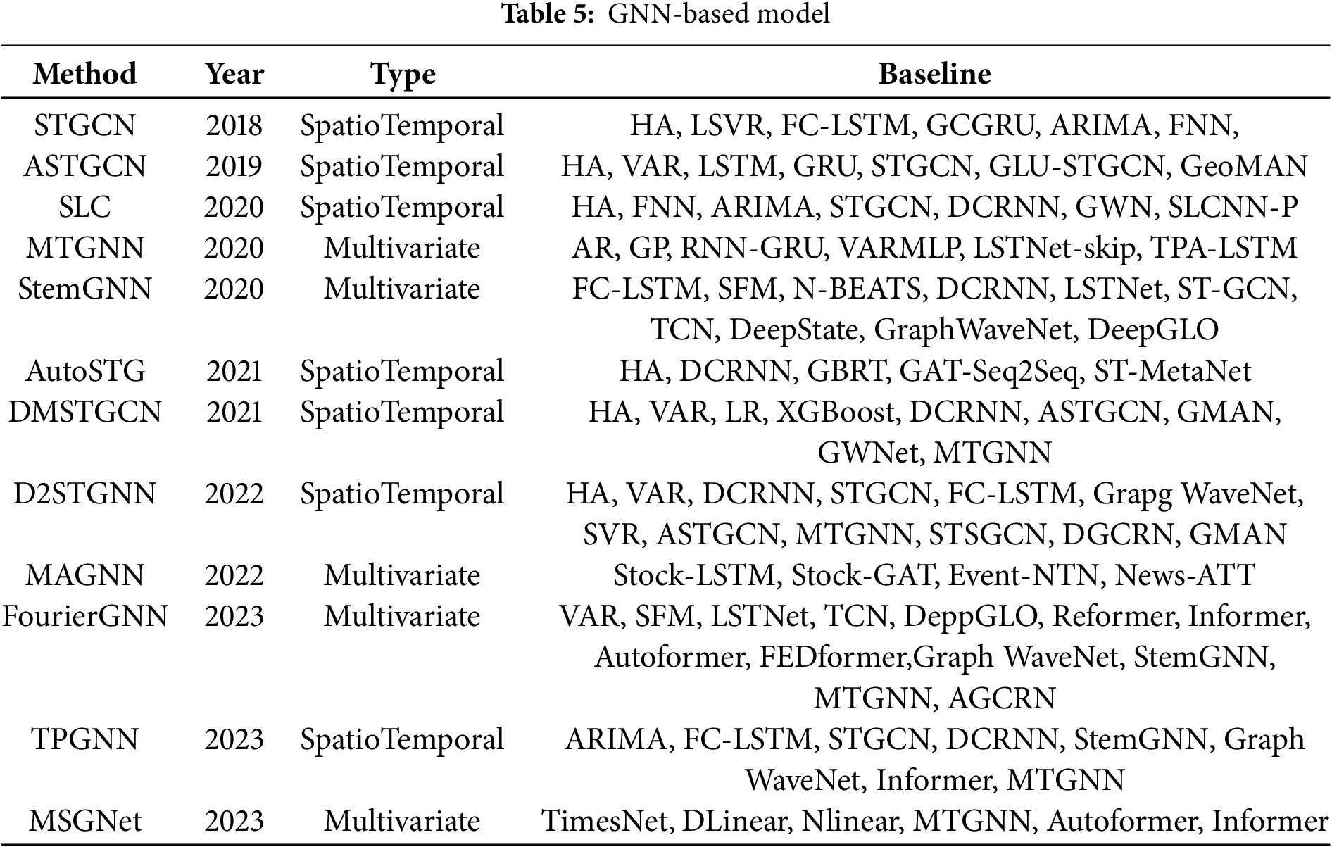
Next, we introduce some GNN-based TSF methods, as shown in Table 5.

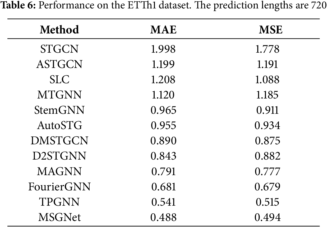
As shown in Table 6, we evaluate the overall performance of the model on the ETTh1 dataset with a prediction length of 720.

Yu et al. [43] proposed a spatio-temporal graph convolutional network (STGCN) to address the limitations of traditional methods in medium- and long-term traffic prediction. STGCN models the problem with a complete convolutional structure on the graph, efficiently capturing comprehensive spatio-temporal correlations and outperforming other models on various traffic datasets by modeling the multiscale traffic network. Guo et al. [44] proposed an attention-based spatio-temporal graph convolution network (ASTGCN). ASTGCN consists of three independent components to model the three temporal attributes of the traffic flow: near-term dependency, daily cycle dependency, and weekly cycle dependency [45]. Each component contains a spatio-temporal attention mechanism for capturing dynamic spatio-temporal correlations and spatio-temporal convolution in traffic data, while graph convolution is employed to capture spatial patterns and ordinary standard convolution to describe temporal features [45]. Zhang et al. [46] identified three challenges in traffic data: (1) traffic data is physically associated with a road network and should be formatted as a traffic graph rather than a plain grid-like tensor, (2) traffic data has strong spatial dependencies, and (3) traffic data has strong time dependencies. To address these issues, they proposed a network framework called Structure Learning Convolution (SLC) [47].

Wu et al. [48] proposed a generalized graph neural network framework for multivariate time series data, allowing the model to automatically extract unidirectional relationships between variables and incorporate external factors such as variable attributes [49]. Cao et al. [50] proposed a Spectral Temporal Graph Neural Network (StemGNN) that captures both intra-sequence temporal correlation and inter-sequence correlation to improve the accuracy of multivariate time series prediction.

Pan et al. [51] proposed AutoSTG, a new network for automatic spatio-temporal graph forecasting. With the aim of exploring the inherent dynamics in traffic data such as traffic speed, traffic volume, and multifaceted spatio-temporal features for better prediction of traffic speed, Han et al. [52] proposed a dynamic graph construction method based on Dynamic Graph Neural Networks (DGNN) to learn the time-specific spatial correlations of road segments. Shao et al. [53] proposed a decoupled spatio-temporal framework (DSTF) to address the problem of traffic data containing both diffuse and intrinsic signals. DSTF separates these signals in a data-driven manner and processes them separately. They also proposed Decoupled Dynamic Spatio-Temporal Graph Neural Network (D2STGNN), which captures spatio-temporal correlations and has a dynamic graph learning module [53].

Financial time series analyses are usually characterized by multi-modal flows and overshooting lag effects, and the financial industry needs predictive models that are interpretable and compatible. Based on these needs, Cheng et al. [54] proposed a multimodal graph neural network (MAGNN) for financial time series forecasting. MAGNN constructs a heterogeneous graph network with sources in the financial knowledge graph as nodes and relations as edges [55].

Latent variable correlations for multivariate time series forecasting are more complex, and the dominant approach using GNNs is to represent the correlations as static graphs, but this approach can lead to significant bias due to the fact that correlations in multivariate time data are constantly changing over time. To address this problem, Liu et al. [56] proposed a temporal polynomial graph neural network (TPGNN) for accurate multivariate time series prediction. TPGNN starts with a static matrix to capture overall correlation and constructs a matrix polynomial for each time step using time-varying coefficients and a matrix basis. Cai et al. [57] proposed MSGNet, it employs a self-attention mechanism and an adaptive hybrid graph convolutional layer to learn different inter-sequence correlations within each time scale.

Overall, GNNs enhance the accuracy and robustness of time series forecasts by capturing the spatio-temporal relationships and correlations between multivariate variables using the characteristic representations of nodes and edges in the graph structure.

3.4 Transformer-Based Methods

The Transformer architecture [58], developed for natural language processing, has become a pivotal framework for temporal modeling due to its self-attention mechanism (Fig. 18). Its encoder-decoder structure operates through: (i) hierarchical feature abstraction in the encoder via multi-head attention, and (ii) autoregressive sequence generation in the decoder. This design fundamentally addresses the long-term dependency learning limitations of RNNs by eliminating recurrent connections, thereby preventing gradient vanishing/explosion issues while enabling parallel processing of entire sequences. The model’s capability to simultaneously attend to all temporal positions through attention weights allows direct capture of both local patterns and global trends in time series data, making it particularly effective for applications requiring modeling of extended temporal contexts.

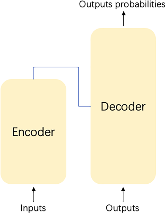
Figure 18: The structure of the Transformer used for the TSF task

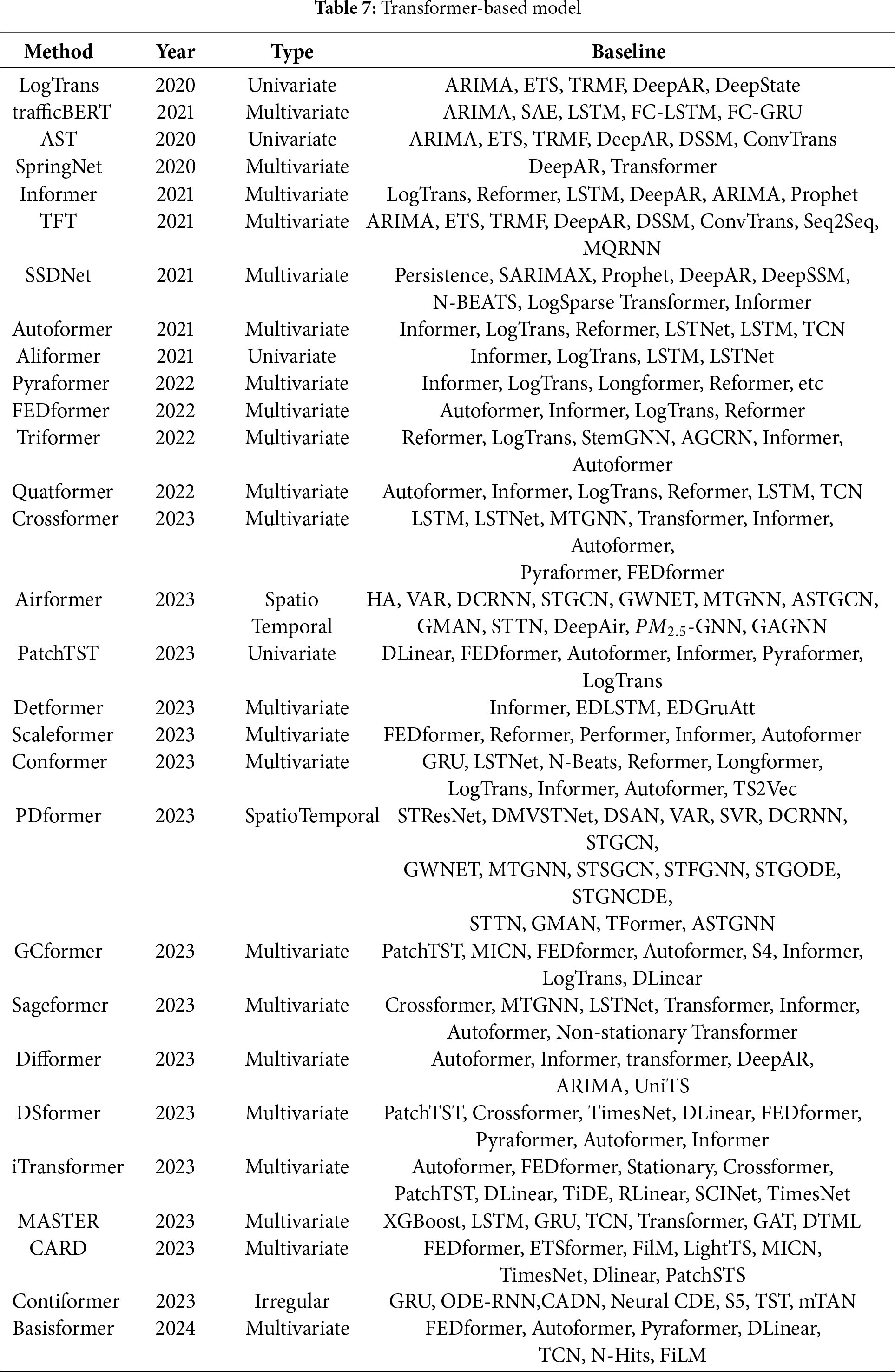
Moreover, compared to RNN models, the self-attention mechanism in Transformer allows for better parallelism and higher computational efficiency. Some applications of Transformer in TSF tasks are presented next, as shown in Table 7.

Li et al. [59] found that Transformer has the problems of limiting diagnosis and memory bottleneck, and to solve these two problems, The authors introduced a novel Convolutional Self-Attention mechanism that revolutionizes traditional attention by employing causal convolutions to generate queries and keys, thereby effectively integrating localized contextual information into the attention computation process. Then, they proposed the LogSparse Transformer with a memory cost of only O(L(log⁡L)2), which improves the prediction accuracy of time series with fine-grained and strong long-term dependencies under a limited memory budget [60].

Jin et al. [61] proposed trafficBERT based on the BERT [13] model. This model captures time series information by using multi-head self-attention instead of the commonly used RNN [61]. The model requires only information about traffic speeds and roads on days of the week for prediction and does not require information about the flow on neighboring roads at the current moment, which has few application limitations.

Tansformer is deficient in facing long sequence time prediction. In terms of this problem, Zhou et al. [62] proposed the Informer model based on the Transformer encoder-decoder structure. The Informer model can give all the required long sequence prediction results at one time, instead of adopting the method of multiple prediction for prediction. Informer first proposes the ProbSparse self-attention mechanism, which can effectively handle longer sequence input data by replacing the traditional Transformer self-attention in the encoder part by employing the multi-head sparse self-attention [63]. Secondly, it proposed a self-attention refining mechanism, which can greatly reduce the number of layers of the network and improve the robustness of the layer stacking part by extracting the self-attention distillation part of the dominant attention. In addition, the decoder part of the model sets the predicted sequence and the subsequent data to 0 for data masking, and the sequence input requires only one forward step, which effectively avoids error accumulation. Informer introduces sparse bias in the self-attention model, as well as Logsparse masking, which reduces the computational complexity of the traditional Transformer model from O(L2) to O(Llog⁡L).

Lim et al. [64] proposed the Time Fusion Transformer (TFT), which uses a recurrent layer for localization and an interpretable self-attentive layer to capture long-term dependencies of the input sequence data. The model can be used for multilevel prediction with interpretability and high performance. Lin et al. [65] proposed the State Space Decomposition Neural Network (SSDNet) that combines Transformer and State Space Modeling (SSM) with both the high performance of deep learning and the interpretability of SSM [65]. It uses the Transformer architecture to learn temporal patterns and directly estimates the parameters of the SSM [65]. Wu et al. [66] proposed Autoformer based on the Transformer model. which transforms Transformer into a decomposition prediction architecture by embedding decomposition blocks as internal operators into the network structure. The model replaces Transformer’s self-attention mechanism with autocorrelation mechanism, which can discover sequence similarity from sequence periodicity. Qi et al. [67] proposed a bi-directional Transformer, Aliformer, for dealing with time series sales forecasting problems in e-commerce. The model is designed with a knowledge-guided self-attentive layer and utilizes historical information, current factors and future knowledge to predict future data changes.

Liu et al. [68] proposed Pyraformer to capture a wide range of temporal dependencies [69]. The method introduces a Pyramid Attention Module (PAM) [70] in which a cross-scale tree structure generalizes features at different resolutions, while intra-scale neighbor connections model different ranges of temporal dependencies [69]. Recent advances in Transformer-based time series forecasting have addressed two critical challenges: computational efficiency and global pattern capture. Pyraformer demonstrates superior performance in empirical evaluations, achieving optimal prediction accuracy with minimal computational overhead—particularly for long-sequence scenarios in both single-step and extended-horizon forecasting tasks. Building on this progress, Zhou et al. [71] introduced FEDformer, which enhances the standard Transformer architecture through: (i) a frequency-domain decomposition strategy to reduce computational complexity, and (ii) specialized Fourier and wavelet enhancement modules that replace conventional attention mechanisms. These innovations collectively enable more efficient modeling of global temporal structures while maintaining competitive predictive performance, as validated through comprehensive benchmarks on large-scale datasets.

A new attention-based Transformer model, Triformer, was proposed by Cirstea et al. [72]. They first proposed an attention mechanism called Patch Attention and designed a new triangular structure that stacks the attention layers, resulting in a significant reduction in the number of layers. In addition, they propose a lightweight method for modeling specific variables by introducing different projection matrices, which can capture different temporal patterns and improve prediction accuracy.

Chen et al. [73] proposed an innovative time series forecasting framework, Quatformer, which handles complex periodic patterns by introducing quaternion-based Learned Rotational Attention (LRA), and tackles the challenges of long-term dependencies and dot-product attention through trend normalization and global memory decoupling. In evaluations on multiple real-world datasets, Quatformer demonstrates its strengths in time series forecasting by improving performance by an average of 8.1% compared to state-of-the-art benchmark models, with up to 18.5% MSE improvement. Recent advancements in Transformer-based time series forecasting have introduced innovative architectures to address spatiotemporal dependencies. Crossformer effectively preserves temporal and dimensional information through its two-stage attention (TSA) layer, which captures cross-time and cross-variable relationships, while its hierarchical encoder-decoder (HED) leverages multi-scale representations for enhanced prediction accuracy, outperforming existing methods across six real-world benchmarks. Similarly, Liang et al. [74] developed Airformer for large-scale air quality forecasting, employing a two-stage framework that combines deterministic spatiotemporal attention with stochastic uncertainty modeling to achieve 5%–8% error reduction in 72-h predictions across thousands of Chinese monitoring stations. These models demonstrate the growing capability of attention-based architectures to handle complex real-world forecasting tasks through specialized mechanisms for dependency modeling and multi-scale feature utilization.

Nie et al. [75] present PatchTST, it significantly improves the accuracy of long-term forecasts by splitting time series into patches with shared embeddings and weights. Meng et al. [76] proposed Detformer, which solves the problem that the Transformer-based method does not have the ability of temporal modeling resulting in the model not being directly applied. The method proposes a dual-feedback sparse attention mechanism to improve the stability of heuristic sparse attention. Also, they designed a time-dependent extraction mechanism to model the perspective of the attention index [76]. In addition, they proposed an algorithm to eliminate data noise so as to optimize the spatio-temporal modeling. Shabani et al. [77] propose ScaleFormer, a generalized multi-scale Transformer framework that enhances existing architectures through three key innovations: (1) iterative multi-scale refinement of predictions using weight-sharing mechanisms to maintain parameter efficiency, (2) strategic architectural modifications for improved temporal representation learning, and (3) a novel normalization scheme specifically optimized for multi-scale processing. This unified approach demonstrates consistent performance improvements across diverse Transformer variants and datasets while introducing minimal computational overhead, effectively addressing the trade-off between model capacity and efficiency in time series forecasting tasks. The framework’s adaptability is further evidenced by its ability to enhance both local pattern capture and global trend modeling through its hierarchical refinement process.

Li et al. [78] proposed Conformer based on Transformer, which is specialized for long-term time series forecasting applications (LTTF) such as wind supply planning. The method achieves higher information utilization and accuracy and is capable of generating reliable forecasts with uncertainty quantification by introducing innovative designs such as an encoder-decoder architecture, a regularized flow module, and explicitly modeling the correlation and dynamics of the time series. Jiang et al. [79] proposed PDformer for accurate traffic flow prediction. Compared with traditional GNN models, PDformer features breakthrough innovations in modeling the spatio-temporal dependencies of urban traffic data, including dynamic spatial dependency capture, long-range spatial dependency modeling, and consideration of propagation time delay of traffic conditions. After extensive experimental validation, PDformer is not only state-of-the-art in terms of performance, but also competitively computationally efficient and makes its model highly interpretable by visualizing spatio-temporal attention maps.

Zhao et al. [80] proposed GCformer, a model that combines a global convolutional branch and a local Transformer branch, to address the limitations of Transformer in the prediction of long-input time series. Zhang et al. [81] proposed Sageformer. As a graph-enhanced Transformer model, Sageformer efficiently captures complex relationships within and between sequences and reduces redundant information.

Li et al. [82] present an effective and efficient Transformer architecture called DifFormer for performing various time series analysis tasks. Compared to previous Transformer variants, DifFormer employs a novel multi-resolution differencing mechanism that is capable of progressively and adaptively highlighting subtle but meaningful variations and is flexible enough to capture periodic or cyclic patterns [82]. Yu et al. [83] proposed a two-sampling transformer model called DSformer for long-term forecasting of multivariate time series.

Liu et al. [84] proposed iTransformer, a time series forecasting model based on the Transformer architecture. By applying attention and feedforward networks on the inverted dimension, iTransformer is able to better capture correlations between multivariate variables and learn nonlinear representations. Experimental results show that iTransformer achieves state-of-the-art performance on real datasets, providing better performance and generalization capabilities for Transformer models in time series forecasting. Li et al. [85] proposed MASTER (MArkert-Guided Stock TransformER) for stock price forecasting, aiming to solve the forecasting challenges caused by high volatility in the stock market. Unlike existing methods, MASTER efficiently models complex stock correlations by considering both instantaneous and intertemporal stock correlations and using market information for automatic feature selection.

Wang et al. [86] proposed the Channel Aligned Robust Blend Transformer (CARD) to address limitations of channel-independent Transformers in time series forecasting. The model introduces three key innovations: (1) a channel-aligned attention mechanism that simultaneously captures inter-variable dependencies and temporal correlations, (2) a multi-scale token mixing module that generates hierarchical representations at varying resolutions, and (3) a novel robust loss function incorporating uncertainty-weighted temporal importance to prevent overfitting. The framework effectively balances the modeling of cross-channel relationships with temporal dynamics while maintaining robustness through its specialized loss formulation.

Recent advances in Transformer-based time series forecasting have introduced innovative architectures to address key challenges in irregular and continuous-time data modeling. Chen et al. [87] developed ContiFormer, which integrates Neural ODE’s continuous dynamics modeling with Transformer attention mechanisms to effectively handle irregular temporal patterns, demonstrating superior performance in continuous-time scenarios. Complementing this approach, Ni et al. [88] proposed BasisFormer, an interpretable framework that leverages self-learned basis functions through adaptive self-supervised learning. By employing bidirectional cross-attention to compute similarity coefficients between historical patterns and basis functions, BasisFormer achieves state-of-the-art performance with 11.04% to 15.78% improvements in univariate and multivariate forecasting tasks respectively across six benchmark datasets. These models collectively advance time series forecasting by combining the relational modeling strengths of Transformers with specialized mechanisms for continuous-time dynamics (ContiFormer) and interpretable pattern decomposition (BasisFormer), while addressing both irregular sampling and prediction accuracy challenges.

In summary, Transformer can capture long-term dependencies well and handle multivariate time series data, and the TSF method based on it has good robustness and generalization ability. It is worth noting that the processing effect of Transformer may be different when facing different time series datasets. Therefore, when dealing with the TSF task, the model selection should be based on the characteristics of the data.

3.5 Recent Advances

Diffusion-Based Forecasting for Time Series: Diffusion models learn data distributions by gradually adding and removing noise, and have recently been successfully applied to time series forecasting. These methods are especially suitable for high-uncertainty domains such as finance and healthcare, as they can generate multiple possible future trajectories, thereby quantifying prediction uncertainty. For example, TimeGrad uses RNNs to encode time series features and then generates probabilistic forecasts through the diffusion process. Recent research like DiffTS further combines diffusion models with Transformers, leveraging self-attention to capture long-term dependencies while retaining the generative capabilities of diffusion models. Additionally, it highlights the need for interpretability in finance, so the generative process of diffusion models should be combined with attention mechanisms or other interpretability tools to enhance trustworthiness.

Hybrid Classical Statistical and Deep Learning Pipelines: Hybrid approaches combine traditional statistical models (such as ARIMA, GARCH) with deep learning models (such as LSTM, Transformer), improving forecasting performance while maintaining interpretability. For example, DeepAR uses autoregressive models to handle linear trends and then applies RNNs to learn nonlinear residuals; N-BEATS dynamically adjusts model weights via interpretable basis expansion modules. Such methods naturally satisfy the explainable AI (XAI) requirements described, since the statistical components provide clear parameter explanations and the deep learning parts can be further analyzed with tools like SHAP.

Quantile Regression Combined with Transformers: Quantile regression directly predicts intervals at different confidence levels (e.g., 5%, 50%, 95% quantiles), providing richer information for financial risk management and decision-making. Transformers, with their powerful sequence modeling capabilities, serve as an ideal framework. For instance, Informer employs quantile attention heads to output multiple quantile forecasts simultaneously, avoiding strong assumptions about data distributions inherent in traditional methods. FEDformer further decomposes time series in the frequency domain and performs quantile regression on each subcomponent, better handling periodicity and sudden events.

4  Datasets and Performance Evaluation Metrics

This section provides an overview of datasets and performance evaluation metrics commonly used in time series forecasting (TSF) tasks. Section 4.1 introduces benchmark datasets across various application domains, summarized in tabular form.

Section 4.2 discusses strategies for training and validating TSF models, with a focus on splitting data into training, validation, and test sets, as well as cross-validation techniques tailored for time series. Section 4.3 explains the importance of using specialized cross-validation techniques like TimeSeriesSplit and Walk-Forward Validation for accurately assessing time series models while maintaining the integrity of temporal dependencies. Section 4.4 addresses strategies for handling data imbalances and outliers in time series, emphasizing preprocessing techniques like robust scaling, outlier detection, and careful treatment of rare events to ensure accurate model performance. Section 4.5 highlights the role of data augmentation in time series forecasting, discussing methods like time warping, jittering, and bootstrapping to artificially expand the dataset and improve model generalization. (R2.18: Sections 4.2–4.5 are additions made in response to the reviewer’s comments). Section 4.6 discusses widely adopted performance evaluation metrics for assessing TSF models.

4.1 Datasets for TSF

The selection and preparation of datasets are critical for algorithm validation, model comparison, and research analysis in TSF. Prior to utilization, datasets typically undergo preprocessing steps such as subset selection, noise reduction, missing value imputation. When addressing real-world problems, it is essential to select appropriate prediction models and algorithms based on the specific characteristics and requirements of the dataset. Blindly adopting state-of-the-art algorithms without considering the problem context may lead to suboptimal results. Researchers should carefully evaluate the number of feature variables, the required prediction horizon, and the scale of the dataset (e.g., the order of magnitude of records) when designing TSF solutions. Below, we describe datasets commonly used in TSF tasks across different application domains.

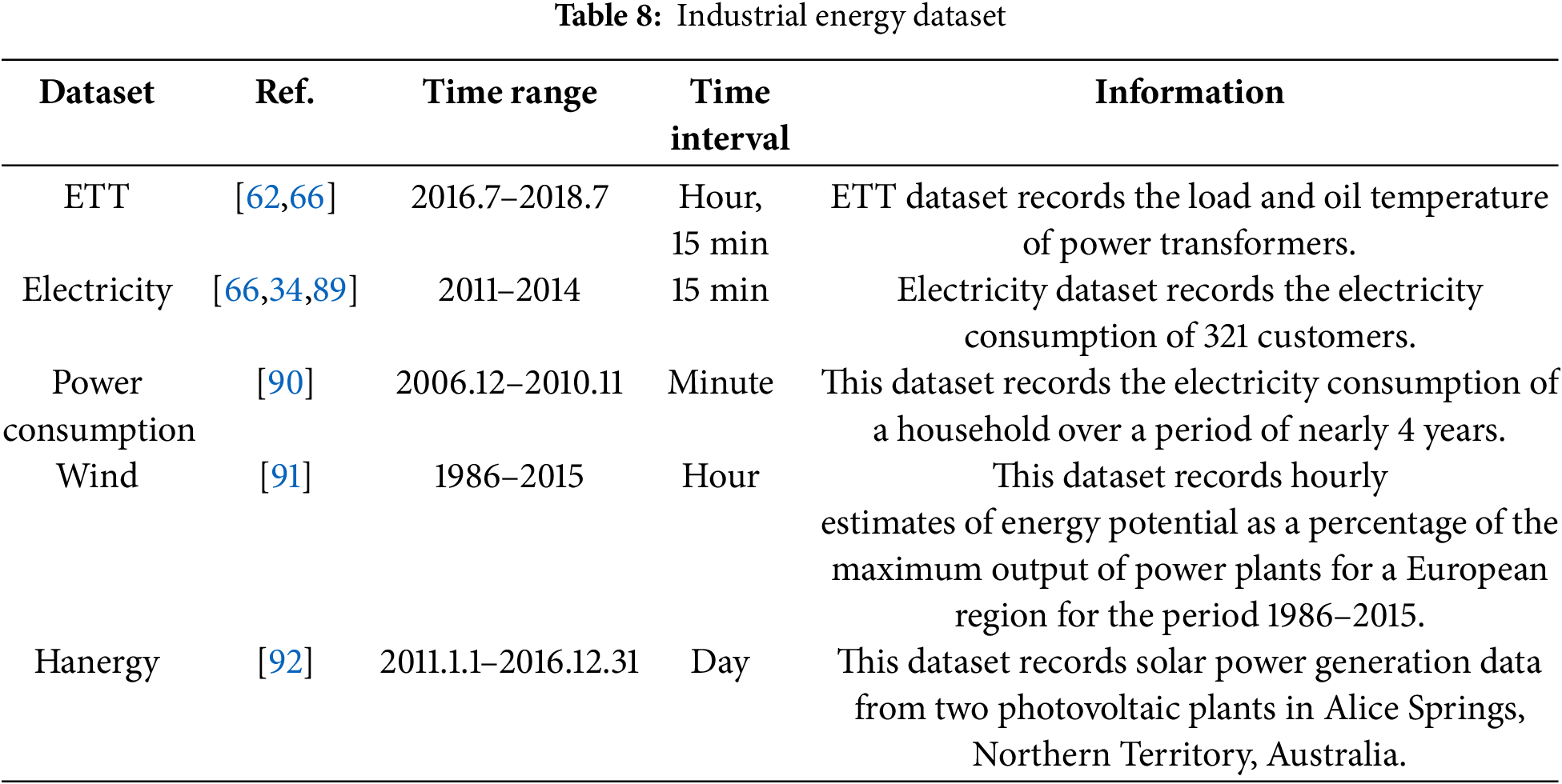
1.   Industrial Energy Datasets

In the industrial energy sector, TSF plays a pivotal role in long-term strategic resource planning. It enables the prediction of future energy demand (e.g., electricity, oil, and natural gas), facilitating optimized production and supply planning. Additionally, TSF assists power companies in forecasting future power generation to ensure stable and adequate supply. These capabilities have broad applications, helping organizations and governments improve planning, mitigate risks, enhance efficiency, and achieve sustainable development goals. Table 8 summarizes key datasets relevant to industrial energy forecasting.

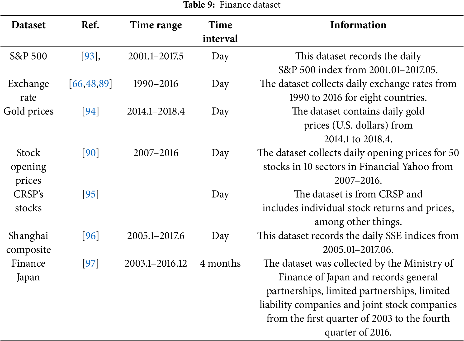
2.   Financial Datasets

TSF is extensively applied in finance, including the prediction of economic cycles, fiscal trends, and stock market behavior. These forecasts provide valuable decision support for financial traders, businesses, and policymakers. In stock markets, TSF models predict price trends and fluctuations, aiding investors in developing robust investment strategies. Beyond market analysis, TSF supports financial institutions in revenue and expenditure planning, loan risk assessment, and interest rate forecasting, thereby informing monetary policy formulation. Table 9 presents a summary of widely used financial datasets.

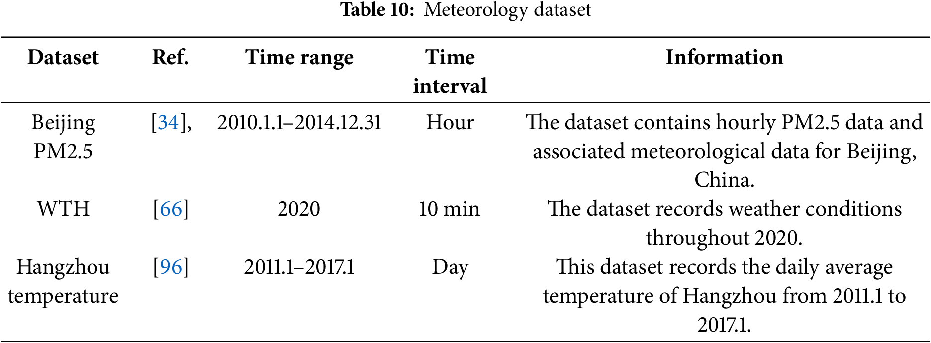
3.   Meteorological Datasets

In meteorology, TSF is employed for long-term climate trend prediction, natural disaster early warning, and marine weather forecasting. These applications provide critical decision support for agriculture, marine transportation, and disaster management, while also contributing to national climate change adaptation strategies. Table 10 summarizes key meteorological datasets used in TSF research.

4.2 Dividing the Dataset into Training, Validation, and Test Subsets

One of the most critical aspects of building forecasting models is the proper division of data into training, validation, and test sets. This division is essential for evaluating the model’s ability to generalize to unseen data and ensuring that it does not overfit.

•   Training Set: The training subset serves as the foundation for developing the forecasting model, enabling it to learn latent patterns and temporal dependencies within the data. For effective time series forecasting, the training period must be carefully selected to encompass a sufficiently extensive duration that captures all critical temporal characteristics.

•   Validation Set: The validation set serves a critical role in model development by enabling hyperparameter optimization (e.g., network depth, learning rate schedules) and model selection. This intermediate dataset provides an unbiased performance assessment during iterative training, acting as an early stopping mechanism to mitigate overfitting while ensuring the model generalizes well to unseen data.

•   Test Set: The test set serves as the gold standard for evaluating model performance, exclusively employed after completing all training and validation phases. This carefully withheld dataset simulates real-world deployment conditions by providing completely unseen data, enabling rigorous assessment of the model’s generalization capacity.

4.3 Cross-Validation Techniques for Time Series

Traditional cross-validation techniques, such as k-fold cross-validation, are not always suitable for time series data due to the temporal dependencies. Instead, methods like TimeSeriesSplit or Walk-Forward Validation are preferred. These techniques involve using earlier data to predict later data while maintaining the temporal structure, ensuring that the validation process mimics the real-world forecasting scenario.

•   TimeSeriesSplit: This method involves splitting the data into several folds, where each fold is used as a validation set in turn, while the training set grows progressively larger with each fold. This allows the model to be trained on more data while still being validated on unseen data.

•   Walk-Forward Validation: In this method, the model is trained on the first portion of the time series, and then tested on the subsequent portion. The process is repeated by moving the training and testing windows forward in time.

4.4 Handling Data Imbalances and Outliers

In time series data, imbalances and outliers can often skew model performance. For instance, rare events (e.g., sudden stock market crashes or natural disasters) may disproportionately affect the dataset. Handling such events requires careful preprocessing, including the use of robust scaling, outlier detection, and data augmentation techniques. Moreover, these rare events should be treated with caution during validation to avoid misleading results.

4.5 Data Augmentation for Time Series

To enhance model robustness and performance, especially when the dataset is small, data augmentation techniques can be employed. For time series forecasting, this might include methods like:

•   Time Warping: Randomly stretching or compressing the time axis to generate new variations of the original time series.

•   Jittering: Adding small random noise to the data to simulate different scenarios.

•   Bootstrapping: Creating synthetic time series by resampling with replacement from the original data.

These techniques help to artificially enlarge the dataset, allowing the model to learn more diverse patterns and improve generalization.

4.6 Performance Evaluation Metrics for Time Series Forecasting (TSF)

In TSF, evaluation metrics serve as crucial tools. These metrics enable us to assess the forecasting capabilities of various models. By leveraging these metrics, we can objectively compare the performance of different models and identify the one that best addresses real-world problems. They provide a standardized approach to measuring a model’s accuracy and precision, facilitating the selection of the most suitable model for predicting future time series data. The insights derived from these metrics allow us to choose the optimal model, thereby enhancing the effectiveness of practical applications. This section presents several widely used evaluation metrics for TSF tasks.

1.   Mean Square Error (MSE)

MSE [98] is defined as the average of the squared differences between predicted and actual values. The formula is as follows:

MSE(y,y^)=1m∑i=1m(yi−y^i)2(14)

where yi represents the true value, y^i represents the predicted value, and m denotes the number of samples.

2.   Root Mean Square Error (RMSE)

RMSE [99] is the square root of the MSE. A smaller RMSE value reflects better predictive capabilities of the model [100]. The calculation formula for RMSE is:

RMSE(y,y^)=1m∑i=1m(yi−y^i)2(15)

where yi denotes the true value, y^i represents the predicted value, and m denotes the number of samples.

3.   Mean Absolute Error (MAE)

MAE [101] is the average of the absolute differences between predicted and actual values. A smaller MAE value indicates enhanced predictive ability of the model [100]. The formula for MAE is presented below:

MAE(y,y^)=1m∑i=1m(|yi−y^i|)(16)

where yi denotes the true value, y^i represents the predicted value, and m denotes the number of samples.

4.   Mean Absolute Percentage Error (MAPE)

MAPE [102] is the average of the absolute percentage.

MAPE(y,y^)=1m∑i=1m|yi−yi^yi|×100%(17)

where yi denotes the true value, y^i represents the predicted value, and m denotes the number of samples.

5  Conclusion and Future Directions

This paper provides an in-depth exploration of the fundamental concepts and definitions related to time series forecasting. By categorizing TSF algorithms based on their underlying network structures, we have divided them into four main categories: CNN-based models, RNN-based models, GNN-based models, and Transformer-based models. We have elaborated on the concepts, principles, and applications of these models and reviewed the state-of-the-art approaches within each category. Additionally, we have presented commonly used datasets and performance evaluation metrics for TSF tasks.

Looking ahead, it is evident that most current TSF models are primarily designed for sequence data with equal time intervals and lack the capability to handle TSF tasks involving datasets with irregular time intervals. To address this limitation, interpolation, filtering, or other techniques could be integrated into the model architecture to effectively manage TSF problems with unequal time intervals. Furthermore, incorporating domain knowledge and considering external privacy factors into time series forecasting models can enhance the accuracy and interpretability of the predictions. These advancements hold significant potential for further improving the performance and applicability of TSF models in real-world scenarios.

Acknowledgement: The authors received no specific support for this study.

Funding Statement: This research was funded by Natural Science Foundation of Heilongjiang Province, grant number LH2023F020.

Author Contributions: The authors confirm contribution to the paper as follows: Conceptualization, Gaoyong Lu and Wei Li; methodology, Yang Ou and Zhihong Wang; software, Zhihong Wang and Yingnan Qu; validation, Yingsheng Xia, Dibin Tang and Zhihong Wang; formal analysis, Igor Kotenko; investigation, Wei Li; resources, Gaoyong Lu; data curation, Yang Ou; writing—original draft preparation, Zhihong Wang and Yingnan Qu; writing—review and editing, Gaoyong Lu and Wei Li; visualization, Yingsheng Xia and Dibin Tang; supervision, Wei Li; project administration, Gaoyong Lu; funding acquisition, Wei Li. All authors reviewed the results and approved the final version of the manuscript.

Availability of Data and Materials: Data available on request from the authors.

Ethics Approval: Not applicable.

Conflicts of Interest: The authors declare no conflicts of interest to report regarding the present study.

References

1. Kim KJ. Financial time series forecasting using support vector machines. Neurocomputing. 2003;55(1–2):307–19. doi:10.1016/S0925-2312(03)00372-2. [Google Scholar] [CrossRef]

2. Kaastra I, Boyd M. Designing a neural network for forecasting financial and economic time series. Neurocomputing. 1996;10(3):215–36. doi:10.1016/0925-2312(95)00039-9. [Google Scholar] [CrossRef]

3. Cao J, Li Z, Li J. Financial time series forecasting model based on CEEMDAN and LSTM. Phys A Stat Mech Appl. 2019;519:127–39. doi:10.1016/j.physa.2018.11.061. [Google Scholar] [CrossRef]

4. Li YF, Dong B, Khan L, Thuraisingham B, Brandt PT, D’Orazio VJ. Data-driven time series forecasting for social studies using spatio-temporal graph neural networks. In: Proceedings of the 2021 Conference on Information Technology for Social Good; 2021 Sep 9–11; Rome, Italy. p. 61–6. doi:10.1145/3462203.3475929. [Google Scholar] [CrossRef]

5. Taylor CJ, Pedregal DJ, Young PC, Tych W. Environmental time series analysis and forecasting with the captain toolbox. Environ Modell Softw. 2007;22(6):797–814. doi:10.1016/j.envsoft.2006.03.002. [Google Scholar] [CrossRef]

6. Murat M, Malinowska I, Gos M, Krzyszczak J. Forecasting daily meteorological time series using ARIMA and regression models. Int Agrophys. 2018;32(2):253–64. doi:10.1515/intag-2017-0007. [Google Scholar] [CrossRef]

7. Zheng J, Huang M. Traffic flow forecast through time series analysis based on deep learning. IEEE Access. 2020;8:82562–70. doi:10.1109/ACCESS.2020.2990738. [Google Scholar] [CrossRef]

8. Lippi M, Bertini M, Frasconi P. Short-term traffic flow forecasting: an experimental comparison of time-series analysis and supervised learning. IEEE Trans Intell Transp Syst. 2013;14(2):871–82. doi:10.1109/TITS.2013.2247040. [Google Scholar] [CrossRef]

9. Chen Z, Ma M, Li T, Wang H, Li C. Long sequence time-series forecasting with deep learning: a survey. Inf Fusion. 2023;97:101819. doi:10.1016/j.inffus.2023.101819. [Google Scholar] [CrossRef]

10. Liu Z, Wang C, Yang X, Zhang N, Liu F, Zhang B. Time series multi-step forecasting based on memory network for the prognostics and health management in freight train braking system. IEEE Trans Intell Transp Syst. 2023;24(8):8149–62. doi:10.1109/TITS.2023.3266227. [Google Scholar] [CrossRef]

11. Noble WS. What is a support vector machine? Nat Biotechnol. 2006;24(12):1565–7. [Google Scholar] [PubMed]

12. Eddy SR. Hidden markov models. Curr Opin Struct Biol. 1996;6(3):361–5. doi:10.1016/S0959-440X(96)80056-X. [Google Scholar] [PubMed] [CrossRef]

13. Devlin J, Chang MW, Lee K, Toutanova K. Bert: pre-training of deep bidirectional transformers for language understanding. arXiv:1810.04805. 2018. doi:10.48550/arXiv.1810.04805. [Google Scholar] [CrossRef]

14. Hewamalage H, Bergmeir C, Bandara K. Recurrent neural networks for time series forecasting: current status and future directions. Int J Forecast. 2021;37(1):388–427. doi:10.1016/j.ijforecast.2020.06.008. [Google Scholar] [CrossRef]

15. Benidis K, Rangapuram SS, Flunkert V, Wang Y, Maddix D, Turkmen C, et al. Deep learning for time series forecasting: tutorial and literature survey. ACM Comput Surv. 2022;55(6):1–36. doi:10.1145/3533382. [Google Scholar] [CrossRef]

16. Kim J, Kim H, Kim H, Lee D, Yoon S. A comprehensive survey of time series forecasting: architectural diversity and open challenges. arXiv:2411.05793. 2024. doi:10.48550/arXiv.2411.05793. [Google Scholar] [CrossRef]

17. Bai S, Kolter JZ, Koltun V. An empirical evaluation of generic convolutional and recurrent networks for sequence modeling. arXiv:1803.01271. 2018. doi:10.48550/arXiv.1803.01271. [Google Scholar] [CrossRef]

18. Li L, Ota K, Dong M. Everything is image: CNN-based short-term electrical load forecasting for smart grid. In: 2017 14th International Symposium on Pervasive Systems, Algorithms and Networks & 2017 11th International Conference on Frontier of Computer Science and Technology & 2017 Third International Symposium of Creative Computing (ISPAN-FCST-ISCC); 2017 Jun 21–23; Exeter, UK. p. 344–51. [Google Scholar]

19. Borovykh A, Bohte S, Oosterlee CW. Conditional time series forecasting with convolutional neural networks. arXiv:1703.04691. 2017. doi:10.48550/arXiv.1703.04691. [Google Scholar] [CrossRef]

20. Dong X, Qian L, Huang L. Short-term load forecasting in smart grid: a combined CNN and K-means clustering approach. In: 2017 IEEE International Conference on Big Data and Smart Computing (BigComp); 2017 Feb 13–16; Jeju Island, Republic of Korea. p. 119–25. [Google Scholar]

21. Cheng J, Huang K, Zheng Z. Towards better forecasting by fusing near and distant future visions. In: Proceedings of the 2020 AAAI Conference on Artificial Intelligence; 2020 Feb 7–12; New York, NY, USA. p. 3593–600. doi:10.1609/aaai.v34i04.5766. [Google Scholar] [CrossRef]

22. Liu M, Zeng A, Chen M, Xu Z, Lai Q, Ma L, et al. Scinet: time series modeling and forecasting with sample convolution and interaction. Adv Neural Inf Process Syst. 2022;35:5816–28. doi:10.48550/arXiv.2106.09305. [Google Scholar] [CrossRef]

23. Wang H, Peng J, Huang F, Wang J, Chen J, Xiao Y. Micn: multi-scale local and global context modeling for long-term series forecasting. In: The Eleventh International Conference on Learning Representations; 2023 May 1–5; Kigali, Rwanda. p. 1–22. [Google Scholar]

24. Wu H, Hu T, Liu Y, Zhou H, Wang J, Long M. Timesnet: temporal 2D-variation modeling for general time series analysis. arXiv:2210.02186. 2022. doi:10.48550/arXiv.2210.02186. [Google Scholar] [CrossRef]

25. Lai Z, Zhang D, Li H, Jensen CS, Lu H, Zhao Y. Lightcts: a lightweight framework for correlated time series forecasting. Proc ACM Manag Data. 2023;1(2):125. doi:10.1145/3589270. [Google Scholar] [CrossRef]

26. Luo D, Wang X. Cross-LKTCN: modern convolution utilizing cross-variable dependency for multivariate time series forecasting dependency for multivariate time series forecasting. arXiv:2306.02326. 2023. doi:10.48550/arXiv.2306.02326. [Google Scholar] [CrossRef]

27. Gong Z, Tang Y, Liang J. Patchmixer: a patch-mixing architecture for long-term time series forecasting. arXiv:2310.00655. 2023. doi:10.48550/arXiv.2310.00655. [Google Scholar] [CrossRef]

28. Luo D, Wang X. Moderntcn: a modern pure convolution structure for general time series analysis. In: The Twelfth International Conference on Learning Representations; 2024 May 7–11; Vienna, Austria. p. 1–43. [Google Scholar]

29. Elman JL. Finding structure in time. Cogn Sci. 1990;14(2):179–211. doi:10.1016/0364-0213(90)90002-E. [Google Scholar] [CrossRef]

30. Graves A. Long short-term memory. Supervised sequence labelling with recurrent neural networks. Berlin/Heidelberg, Germany: Springer; 2012. p. 37–45. doi:10.1007/978-3-642-24797-2_4. [Google Scholar] [CrossRef]

31. Cho K, Van Merriënboer B, Gulcehre C, Bahdanau D, Bougares F, Schwenk H, et al. Learning phrase representations using RNN encoder-decoder for statistical machine translation. arXiv:1406.1078. 2014. doi:10.48550/arXiv.1406.1078. [Google Scholar] [CrossRef]

32. Lai G, Chang WC, Yang Y, Liu H. Modeling long-and short-term temporal patterns with deep neural networks. In: The 41st International ACM SIGIR Conference on Research & Development in Information Retrieval; 2018 Jul 8–12; Ann Arbor, MI, USA. p. 95–104. doi:10.48550/arXiv.1703.07015. [Google Scholar] [CrossRef]

33. Qin Y, Song D, Chen H, Cheng W, Jiang G, Cottrell G. A dual-stage attention-based recurrent neural network for time series prediction. arXiv:1704.02971. 2017. doi:10.48550/arXiv.1704.02971. [Google Scholar] [CrossRef]

34. Chang YY, Sun FY, Wu YH, Lin SD. A memory-network based solution for multivariate time-series forecasting. arXiv:1809.02105. 2018. doi:10.48550/arXiv.1809.021057. [Google Scholar] [CrossRef]

35. Fan C, Zhang Y, Pan Y, Li X, Zhang C, Yuan R, et al. Multi-horizon time series forecasting with temporal attention learning. In: Proceedings of the 25th ACM SIGKDD International Conference on Knowledge Discovery & Data Mining; 2019 Aug 4–8; Anchorage, AK, USA. p. 2527–35. doi:10.1145/3292500.3330662. [Google Scholar] [CrossRef]

36. Jung Y, Jung J, Kim B, Han S. Long short-term memory recurrent neural network for modeling temporal patterns in long-term power forecasting for solar PV facilities: case study of South Korea. J Clean Prod. 2020;250:119476. doi:10.1016/j.jclepro.2019.119476. [Google Scholar] [CrossRef]

37. Du S, Li T, Yang Y, Horng SJ. Multivariate time series forecasting via attention-based encoder-decoder framework. Neurocomputing. 2020;388:269–79. doi:10.1016/j.neucom.2019.12.118. [Google Scholar] [CrossRef]

38. Gangopadhyay T, Tan SY, Jiang Z, Meng R, Sarkar S. Spatiotemporal attention for multivariate time series prediction and interpretation. In: ICASSP 2021—2021 IEEE International Conference on Acoustics, Speech and Signal Processing (ICASSP). Piscataway, NJ, USA: IEEE; 2021. p. 3560–4. doi:10.1109/icassp39728.2021.9413914. [Google Scholar] [CrossRef]

39. Schirmer M, Eltayeb M, Lessmann S, Rudolph M. Modeling irregular time series with continuous recurrent units. arXiv:2111.11344. 2022. doi:10.48550/arXiv.2111.11344. [Google Scholar] [CrossRef]

40. Jia Y, Lin Y, Hao X, Lin Y, Guo S, Wan H. Witran: water-wave information transmission and recurrent acceleration network for long-range time series forecasting. In: Advances in neural information processing systems. Red Hook, NY, USA: Curran Associates, Inc.; 2023. p. 12389–456. doi:10.5555/3666122.3666666. [Google Scholar] [CrossRef]

41. Veličković P, Cucurull G, Casanova A, Romero A, Liò P, Bengio Y. Graph attention networks. arXiv:1710.10903. 2018. doi:10.48550/arXiv.1710.10903. [Google Scholar] [CrossRef]

42. Kipf T. Semi-supervised classification with graph convolutional networks. arXiv:1609.02907. 2016. doi:10.48550/arXiv.1609.02907. [Google Scholar] [CrossRef]

43. Yu B, Yin H, Zhu Z. Spatio-temporal graph convolutional networks: a deep learning framework for traffic forecasting. In: Proceedings of the Twenty-Seventh International Joint Conference on Artificial Intelligence. International Joint Conferences on Artificial Intelligence Organization; 2018 Jul 13–19; Stockholm, Sweden. p. 3634–40. doi:10.24963/ijcai.2018/505. [Google Scholar] [CrossRef]

44. Guo S, Lin Y, Feng N, Song C, Wan H. Attention based spatial-temporal graph convolutional networks for traffic flow forecasting. In: Proceedings of the 2019 AAAI Conference on Artificial Intelligence; 2019 Jan 27–Feb 1; Honolulu, HI, USA. p. 922–9. doi:10.1609/aaai.v33i01.3301922. [Google Scholar] [CrossRef]

45. Gao Z, Li Z, Zhang H, Yu J, Xu L. Dynamic spatiotemporal interactive graph neural network for multivariate time series forecasting. Knowl Based Syst. 2023;280:110995. doi:10.1016/j.knosys.2023.110995. [Google Scholar] [CrossRef]

46. Zhang Q, Chang J, Meng G, Xiang S, Pan C. Spatio-temporal graph structure learning for traffic forecasting. In: Proceedings of the AAAI Conference on Artificial Intelligence; 2020 Feb 7–12; New York, NY, USA. p. 1177–85. doi:10.1609/aaai.v34i01.5470. [Google Scholar] [CrossRef]

47. Zhang Q, Chang W, Yin C, Xiao P, Li K, Tan M. Attention-based spatial-temporal convolution gated recurrent unit for traffic flow forecasting. Entropy. 2023;25(6):938. doi:10.3390/e25060938. [Google Scholar] [PubMed] [CrossRef]

48. Wu Z, Pan S, Long G, Jiang J, Chang X, Zhang C. Connecting the dots: multivariate time series forecasting with graph neural networks. In: Proceedings of the 26th ACM SIGKDD International Conference on Knowledge Discovery & Data Mining; 2020 Jul 6–10; Online. p. 753–63. doi:10.1145/3394486.3403118. [Google Scholar] [CrossRef]

49. Ling J, Lan Y, Huang X, Yang X. A multi-scale residual graph convolution network with hierarchical attention for predicting traffic flow in urban mobility. Complex Intell Syst. 2024;10(3):3305–17. doi:10.1007/s40747-023-01324-9. [Google Scholar] [CrossRef]

50. Cao D, Wang Y, Duan J, Zhang C, Zhu X, Huang C, et al. Spectral temporal graph neural network for multivariate time-series forecasting. arXiv:2103.07719. 2021. doi:10.48550/arXiv.2103.07719. [Google Scholar] [CrossRef]

51. Pan Z, Ke S, Yang X, Liang Y, Yu Y, Zhang J, et al. AutoSTG: neural architecture search for predictions of spatio-temporal graph. In: WWW’21: Proceedings of the Web Conference 2021; 2021 Apr 19–23; Ljubljana, Slovenia. p. 1846–55. doi:10.1145/3442381.3449816. [Google Scholar] [CrossRef]

52. Han L, Du B, Sun L, Fu Y, Lv Y, Xiong H. Dynamic and multi-faceted spatio-temporal deep learning for traffic speed forecasting. In: Proceedings of the 27th ACM SIGKDD Conference on Knowledge Discovery & Data Mining; 2021 Aug 14–18; Singapore. p. 547–55. doi:10.1145/3447548.3467275. [Google Scholar] [CrossRef]

53. Shao Z, Zhang Z, Wei W, Wang F, Xu Y, Cao X, et al. Decoupled dynamic spatial-temporal graph neural network for traffic forecasting. Proc VLDB Endow. 2022;15(11):2733–46. doi:10.14778/3551793.3551827. [Google Scholar] [CrossRef]

54. Cheng D, Yang F, Xiang S, Liu J. Financial time series forecasting with multi-modality graph neural network. Pattern Recognit. 2022;121:108218. doi:10.1016/j.patcog.2021.108218. [Google Scholar] [CrossRef]

55. Wang J, Yang S, Zhao H. Crisis event summary generative model based on hierarchical multimodal fusion. Pattern Recognit. 2023;144:109890. doi:10.1016/j.patcog.2023.109890. [Google Scholar] [CrossRef]

56. Liu Y, Liu Q, Zhang JW, Feng H, Wang Z, Zhou Z, et al. Multivariate time-series forecasting with temporal polynomial graph neural networks. Adv Neural Inf Process Syst. 2022;35:19414–26. doi:10.5555/3600270.3601681. [Google Scholar] [CrossRef]

57. Cai W, Liang Y, Liu X, Feng J, Wu Y. Msgnet: learning multi-scale inter-series correlations for multivariate time series forecasting. In: Proceedings of the 2024 AAAI Conference on Artificial Intelligence; 2024 Feb 20–27; Vancouver, BC, Canada. p. 11141–9. doi:10.1609/aaai.v38i10.28991. [Google Scholar] [CrossRef]

58. Vaswani A, Shazeer N, Parmar N, Uszkoreit J, Jones L, Gomez AN, et al. Attention is all you need. In: Advances in neural information processing systems. Cambridge, MA, USA: MIT Press; 2017. Vol. 30. doi:10.48550/arXiv.1706.03762. [Google Scholar] [CrossRef]

59. Li S, Jin X, Xuan Y, Zhou X, Chen W, Wang YX, et al. Enhancing the locality and breaking the memory bottleneck of transformer on time series forecasting. In: Proceedings of the 33rd International Conference on Neural Information Processing Systems; 2019 Dec 8–14; Vancouver, BC, Canada. p. 5243–53. doi:10.5555/3454287.3454758. [Google Scholar] [CrossRef]

60. Li R, Zhang X. All you need is transformer: RTT prediction for TCP based on deep learning approach. In: 2021 International Conference on Digital Society and Intelligent Systems (DSInS); 2021 Nov 19–21; Chengdu, China. p. 348–51. doi:10.1109/dsins54396.2021.9670591. [Google Scholar] [CrossRef]

61. Jin K, Wi J, Lee E, Kang S, Kim S, Kim Y. TrafficBERT: pre-trained model with large-scale data for long-range traffic flow forecasting. Expert Syst Appl. 2021;186:115738. doi:10.1016/j.eswa.2021.115738. [Google Scholar] [CrossRef]

62. Zhou H, Zhang S, Peng J, Zhang S, Li J, Xiong H, et al. Informer: beyond efficient transformer for long sequence time-series forecasting. In: Proceedings of the 35th AAAI Conference on Artificial Intelligence; 2021 Feb 2–9; Online. p. 11106–15. doi:10.1609/aaai.v35i12.17325. [Google Scholar] [CrossRef]

63. Banerjee S, Dong M, Shi W. Spatial-temporal synchronous graph transformer network (STSGT) for COVID-19 forecasting. Smart Health. 2022;26:100348. doi:10.1109/TPAMI.2023.3293516. [Google Scholar] [CrossRef]

64. Lim B, Arık SÖ, Loeff N, Pfister T. Temporal fusion transformers for interpretable multi-horizon time series forecasting. Int J Forecast. 2021;37(4):1748–64. doi:10.1016/j.ijforecast.2021.03.012. [Google Scholar] [CrossRef]

65. Lin Y, Koprinska I, Rana M. SSDNet: state space decomposition neural network for time series forecasting. In: 2021 IEEE International Conference on Data Mining (ICDM); 2021 Dec 7–10; Auckland, New Zealand. p. 370–8. doi:10.48550/arXiv.2112.10251. [Google Scholar] [CrossRef]

66. Wu H, Xu J, Wang J, Long M. Autoformer: decomposition transformers with auto-correlation for long-term series forecasting. Adv Neural Inf Process Syst. 2021;34:22419–30. doi:10.48550/arXiv.2106.13008. [Google Scholar] [CrossRef]

67. Qi X, Hou K, Liu T, Yu Z, Hu S, Ou W. From known to unknown: knowledge-guided transformer for time-series sales forecasting in Alibaba. arXiv:2109.08381. 2021. doi:10.48550/arXiv.2109.08381. [Google Scholar] [CrossRef]

68. Liu S, Yu H, Liao C, Li J, Lin W, Liu AX, et al. Pyraformer: low-complexity pyramidal attention for long-range time series modeling and forecasting. In: International Conference on Learning Representations; 2022 Apr 25–29; Online. p. 1–20. [Google Scholar]

69. Ma S, Guan S, He Z, Nie J, Gao M. TPAD: temporal-pattern-based neural network model for anomaly detection in multivariate time series. IEEE Sens J. 2023;23(24):30668–82. doi:10.1109/JSEN.2023.3327138. [Google Scholar] [CrossRef]

70. Bian Z, Wan Z, Li F, Liu D, Lyu Z. Oil temperature prediction method based on deep learning and digital twins. In: Asian Conference on Pattern Recognition. Cham, Swizterland: Springer; 2023. p. 174–84. doi:10.1007/978-3-031-47665-5_15. [Google Scholar] [CrossRef]

71. Zhou T, Ma Z, Wen Q, Wang X, Sun L, Jin R. Fedformer: frequency enhanced decomposed transformer for long-term series forecasting. In: International Conference on Machine Learning. Westminster, UK: PMLR; 2022. p. 27268–86. doi:10.48550/arXiv.2201.12740. [Google Scholar] [CrossRef]

72. Cirstea R, Guo C, Yang B, Kieu T, Dong X, Pan S. Triformer: triangular, variable-specific attentions for long sequence multivariate time series forecasting. In: The Thirty-First International Joint Conference on Artificial Intelligence (IJCAI-22). International Joint Conference on Artificial Intelligence (IJCAI); 2022 Jul 23–29; Vienna, Austria. p. 1994–2001. doi:10.48550/arXiv.2204.13767. [Google Scholar] [CrossRef]

73. Chen W, Wang W, Peng B, Wen Q, Zhou T, Sun L. Learning to rotate: quaternion transformer for complicated periodical time series forecasting. In: Proceedings of the 28th ACM SIGKDD Conference on Knowledge Discovery and Data Mining; 2022 Aug 14–18; Washington, DC, USA. p. 146–56. doi:10.1145/3534678.3539234. [Google Scholar] [CrossRef]

74. Liang Y, Xia Y, Ke S, Wang Y, Wen Q, Zhang J, et al. Airformer: predicting nationwide air quality in china with transformers. In: Proceedings of the 37th AAAI Conference on Artificial Intelligence; 2023 Feb 7–14; Washington, DC, USA. p. 14329–37. doi:10.1609/aaai.v37i12.26676. [Google Scholar] [CrossRef]

75. Nie Y, Nguyen NH, Sinthong P, Kalagnanam J. A time series is worth 64 words: long-term forecasting with transformers. arXiv:2211.14730. 2022. doi:10.48550/arXiv.2211.14730. [Google Scholar] [CrossRef]

76. Meng X, Li W, Zhao Z, Liu Z, Feng G, Wang H. Detformer: detect the reliable attention index for ultra-long time series forecasting. In: International Conference on Intelligent Computing. Cham, Switzerland: Springer; 2023. p. 457–68. doi:10.1515/intag-2017-0007. [Google Scholar] [CrossRef]

77. Shabani MA, Abdi AH, Meng L, Sylvain T. Scaleformer: iterative multi-scale refining transformers for time series forecasting. arXiv:2206.04038. 2023. doi:10.48550/arXiv.2206.04038. [Google Scholar] [CrossRef]

78. Li Y, Lu X, Xiong H, Tang J, Su J, Jin B, et al. Towards long-term time-series forecasting: feature, pattern, and distribution. In: 2023 IEEE 39th International Conference on Data Engineering (ICDE); 2023 Apr 3–7; Anaheim, CA, USA. p. 1611–24. doi:10.1109/ICDE55515.2023.00127. [Google Scholar] [CrossRef]

79. Jiang J, Han C, Zhao WX, Wang J. Pdformer: propagation delay-aware dynamic long-range transformer for traffic flow prediction. In: Proceedings of the AAAI Conference on Artificial Intelligence; 2023 Feb 7–14; Washington, DC, USA. p. 4365–73. doi:10.1609/aaai.v37i4.25556. [Google Scholar] [CrossRef]

80. Zhao Y, Ma Z, Zhou T, Ye M, Sun L, Qian Y. GCformer: an efficient solution for accurate and scalable long-term multivariate time series forecasting. In: Proceedings of the 32nd ACM International Conference on Information and Knowledge Management; 2023 Oct 21–25; Birmingham, UK. p. 3464–73. doi:10.1145/3583780.361513. [Google Scholar] [CrossRef]

81. Zhang Z, Meng L, Gu Y. SageFormer: series-aware framework for long-term multivariate time-series forecasting. IEEE Internet Things J. 2024;11(10):18435–48. doi:10.1109/JIOT.2024.3363451. [Google Scholar] [CrossRef]

82. Li B, Cui W, Zhang L, Zhu C, Wang W, Tsang IW, et al. DifFormer: multi-resolutional differencing transformer with dynamic ranging for time series analysis. IEEE Trans Pattern Anal Mach Intell. 2023;45(11):13586–98. doi:10.1109/TPAMI.2023.3293516. [Google Scholar] [PubMed] [CrossRef]

83. Yu C, Wang F, Shao Z, Sun T, Wu L, Xu Y. Dsformer: a double sampling transformer for multivariate time series long-term prediction. In: Proceedings of the 32nd ACM International Conference on Information and Knowledge Management; 2023 Oct 21–25; Birmingham, UK. p. 3062–72. doi:10.1145/3583780.361485. [Google Scholar] [CrossRef]

84. Liu Y, Hu T, Zhang H, Wu H, Wang S, Ma L, et al. iTransformer: inverted transformers are effective for time series forecasting. arXiv:2310.06625. 2023. doi:10.48550/arXiv.2310.06625. [Google Scholar] [CrossRef]

85. Li T, Liu Z, Shen Y, Wang X, Chen H, Huang S. Master: market-guided stock transformer for stock price forecasting. In: Proceedings of the AAAI Conference on Artificial Intelligence; 2024 Feb 20–27; Vancouver, BC, Canada. p. 162–70. doi:10.1609/aaai.v38i1.27767. [Google Scholar] [CrossRef]

86. Wang X, Zhou T, Wen Q, Gao J, Ding B, Jin R. CARD: channel aligned robust blend transformer for time series forecasting. arXiv:2305.12095. 2024. doi:10.48550/arXiv.2305.12095. [Google Scholar] [CrossRef]

87. Chen Y, Ren K, Wang Y, Fang Y, Sun W, Li D. ContiFormer: continuous-time transformer for irregular time series modeling. In: Proceedings of the 37th International Conference on Neural Information Processing Systems; 2023 Dec 10–16; New Orleans, LA, USA. p. 47143–75. doi:10.5555/3666122.3668164. [Google Scholar] [CrossRef]

88. Ni Z, Yu H, Liu S, Li J, Lin W. BasisFormer: attention-based time series forecasting with learnable and interpretable basis. In: Proceedings of the 37th International Conference on Neural Information Processing Systems; 2023 Dec 10–16; New Orleans, LA, USA. p. 71222–41. doi:10.5555/3666122.3669240. [Google Scholar] [CrossRef]

89. Yoo J, Kang U. Attention-based autoregression for accurate and efficient multivariate time series forecasting. In: Proceedings of the 2021 SIAM International Conference on Data Mining (SDM); 2021 Apr 29–May 1; Alexandria, VA, USA. p. 531–9. doi:10.1137/1.9781611976700.60. [Google Scholar] [CrossRef]

90. Zhao Y, Shen Y, Zhu Y, Yao J. Forecasting wavelet transformed time series with attentive neural networks. In: 2018 IEEE International Conference on Data Mining (ICDM); 2018 Nov 17–20; Singapore. p. 1452–7. doi:10.1109/ICDM.2018.002017. [Google Scholar] [CrossRef]

91. Wu S, Xiao X, Ding Q, Zhao P, Wei Y, Huang J. Adversarial sparse transformer for time series forecasting. Adv Neural Inf Process Syst. 2020;33:17105–15. doi:10.5555/3495724.3497159. [Google Scholar] [CrossRef]

92. Lin Y, Koprinska I, Rana M. SpringNet: transformer and spring DTW for time series forecasting. In: International Conference on Neural Information Processing. Cham, Swizterland: Springer; 2020. p. 616–28. doi:10.1007/978-3-030-63836-8_51. [Google Scholar] [CrossRef]

93. Yang Z, Yan W, Huang X, Mei L. Adaptive temporal-frequency network for time-series forecasting. IEEE Trans Knowl Data Eng. 2020;34(4):1576–87. doi:10.1109/TKDE.2020.3003420. [Google Scholar] [CrossRef]

94. Livieris IE, Pintelas E, Pintelas P. A CNN-LSTM model for gold price time-series forecasting. Neural Comput Appl. 2020;32:17351–60. doi:10.1007/s00521-020-04867-x. [Google Scholar] [CrossRef]

95. Hou X, Wang K, Zhang J, Wei Z. An enriched time-series forecasting framework for long-short portfolio strategy. IEEE Access. 2020;8:31992–2002. doi:10.1109/access.2020.2973037. [Google Scholar] [CrossRef]

96. Shen Z, Zhang Y, Lu J, Xu J, Xiao G. A novel time series forecasting model with deep learning. Neurocomputing. 2020;396:302–13. doi:10.1016/j.neucom.2018.12.084. [Google Scholar] [CrossRef]

97. Yoshimi S, Eguchi K. Forecasting corporate financial time series using multi-phase attention recurrent neural networks. In: EDBT/ICDT Workshops 2020 [Internet]. [cited 2025 Aug 6]. Available from: http://star.informatik.rwth-aachen.de/Publications/CEUR-WS/Vol-2578/DARLIAP12.pdf. [Google Scholar]

98. Wang Z, Bovik AC. Mean squared error: love it or leave it? A new look at signal fidelity measures. IEEE Signal Process Mag. 2009;26(1):98–117. doi:10.1515/intag-2017-0007. [Google Scholar] [CrossRef]

99. Chai T, Draxler RR. Root mean square error (RMSE) or mean absolute error (MAE)?—Arguments against avoiding RMSE in the literature. Geosci Model Dev. 2014;7(3):1247–50. doi:10.5194/gmd-7-1247-2014. [Google Scholar] [CrossRef]

100. Liu Y, Huang X, Xiong L, Chang R, Wang W, Chen L. Stock price prediction with attentive temporal convolution-based generative adversarial network. Array. 2025;25:100374. doi:10.1016/j.array.2025.100374. [Google Scholar] [CrossRef]

101. Willmott CJ, Matsuura K. Advantages of the mean absolute error (MAE) over the root mean square error (RMSE) in assessing average model performance. Clim Res. 2005;30(1):79–82. doi:10.3354/cr030079. [Google Scholar] [CrossRef]

102. De Myttenaere A, Golden B, Le Grand B, Rossi F. Mean absolute percentage error for regression models. Neurocomputing. 2016;192:38–48. doi:10.1016/j.neucom.2015.12.114. [Google Scholar] [CrossRef]