Mild Cognitive Impairment Detection from Rey-Osterrieth Complex Figure Copy Drawings Using a Contrastive Loss Siamese Neural Network

1  Introduction

The detection of cognitive decline in adults is an increasingly relevant issue in a global context where the number of people with dementia is expected to triple in the next 30 years [1]. When an individual’s decline is greater than expected for their age and education level but does not interfere with their daily activities, it is known as mild cognitive impairment (MCI) [2]. If an individual is diagnosed with MCI, therapies can be activated to slow the onset of dementia, improving their quality of life and that of their caregivers, while also saving medical resources in the long term [3]. Issuing this diagnosis may require the collection of diverse information from the individual, including current symptoms, medical history, biomarkers (from cerebrospinal fluid or plasma), magnetic resonance and molecular imaging data, and neuropsychological test results [4,5]. Machine learning algorithms can aid in the analysis of this information, leading to enhanced clinical decision-making [6–9].

This article focuses on the automatic analysis of neuropsychological tests, since their cost-effectiveness and minimal invasive nature make them ideal early screening tools [10,11]. Each test evaluates different cognitive abilities, and their results are combined by a team of psychologists to determine the cognitive state of a certain individual. Some examples of neuropsychological tests are Test de aprendizaje verbal España-Complutense (TAVEC) [12], which is the Spanish version of the California Verbal Learning Test (CVLT) [13], Trail Making Test (TMT) [14], or Rey-Osterrieth Complex Figure (ROCF) Test [15,16]. The latter has proven to be quite comprehensive, offering insights into an individual’s visuo-spatial ability, executive functions, and memory [17]. This test involves reproducing a line drawing, first by copying it and then from memory. Copying the figure allows for the evaluation of an individual’s constructive and executive skills, while its reproduction through delayed recall also provides information on their visual memory status. The quality of the figure representation is measured using scoring systems like the Quantitative Scoring System (QSS) [15,16,18], which assigns a quantitative value based on the presence, completeness, and positioning of various ROCF components. This value is generally low in individuals with MCI [19], with a particularly clear case being people with frontal lobe lesions [20]. Seo et al. [21] go further, stating that the QSS score could predict whether a healthy individual will transition to a pre-MCI or even MCI state. However, it should be noted that this score is conditioned by the differences in criteria among various experts, as can be deduced from the inter-rater variability study conducted in [22]. These biases in scores could hinder the psychologists’ task of determining an individual’s cognitive state. Therefore, we propose the development of an automatic system that detects the presence of MCI by directly analyzing the ROCF drawing.

This task could be designed as a classification problem, where the input would be an ROCF drawing and the output would be a label with the individual’s cognitive state. This problem is usually solved using deep learning (DL) architectures [23–27], due to their excellent results in image classification over the last decade. These architectures learn the relationship between the input image and the output label through examples, in such a way that they can infer the label of an unseen image. However, for their performance to be adequate, they require a very large number of examples. Since our data availability is limited, we decide to treat the previously mentioned task as a similarity or distance metric learning problem [28,29]. In these problems, pairwise example comparisons are used to generate a metric space that allows images to be separated according to their class. We believe that such comparisons could improve data leverage and class distinction. The models generally used to solve distance metric learning problems are siamese neural networks (SNNs) [30], given their proven performance in tasks like person re-identification [31], image retrieval [32], or image matching [33].

The aim of this article is to examine the effectiveness of SNNs to predict an individual’s cognitive state based on a copy drawing of the ROCF. Our SNN proposal relies on the distance to the ROCF model (an ideal representation of the ROCF) [34] to distinguish between ROCF drawings made by healthy individuals or those diagnosed with MCI. Using a public dataset of copy-extracted ROCF drawings called ROCFD528 [22], a comparative study will be carried out between our model and the DL models from the literature, which are designed to solve a classification problem. The code and data used in this study are publicly available at the following address: https://edatos.consorciomadrono.es/dataverse/rey (accessed on 23 September 2025). However, the diagnoses are confidential and will only be provided upon request.

The article is structured as follows: in Section 2, we will describe the state-of-the-art methods that share our objective of predicting an individual’s cognitive state based on the ROCF; in Section 3, we present our dataset and explain our SNN proposal; in Section 4, we analyze the performance, decision-making logic, size and computational cost of our proposal and three state-of-the-art architectures; in Section 5, we outline some of our limitations and propose future work; finally, in Section 6, we highlight our main contributions.

2  Related Work

There are several recent works that predict an individual’s cognitive state based solely on the ROCF drawing [35–38]. The datasets used include ROCF drawings extracted both by copying and from memory. For each of these drawings, the individual’s cognitive state at the time of the test is recorded. Typically, the states considered are healthy, MCI, or dementia. But, in some cases, MCI subtypes are also taken into account: amnestic (aMCI) or non-amnestic (naMCI), and single-domain or multi-domain. The aMCI subtype implies a significant memory impairment and is often associated with Alzheimer’s disease, while the naMCI subtype affects other cognitive domains and is often related to less common diseases, such as frontotemporal degeneration or Lewy body dementia [39].

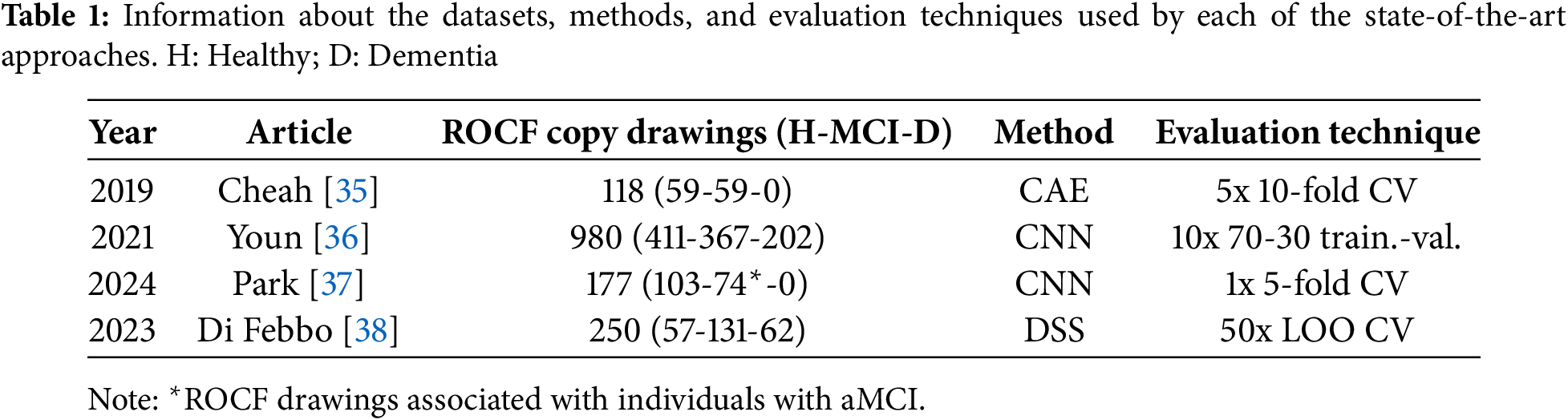
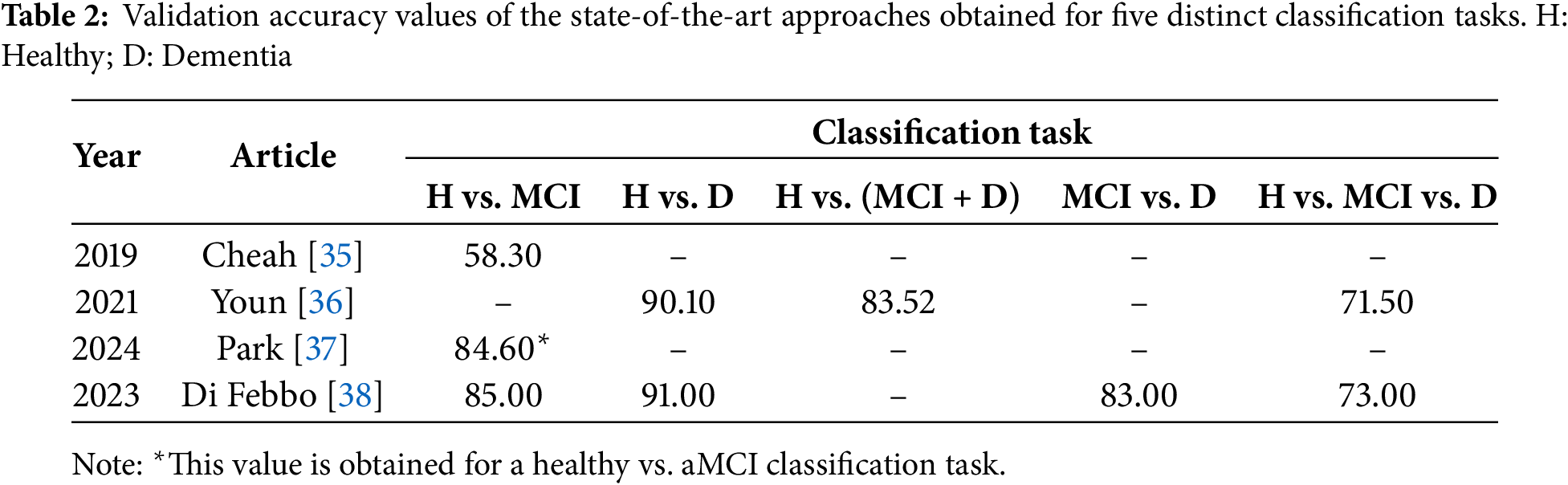
To assign these labels to ROCF drawings, two types of automatic systems are proposed: those based exclusively on DL models [35–37] and those based on decision support systems (DSS) [38]. Focusing on the former, Cheah et al. [35] employ a convolutional auto-encoder (CAE) that extracts a feature vector from the ROCF, and several fully connected layers that associate these features with a healthy or MCI cognitive state. Their dataset includes 118 ROCF copy drawings, corresponding to 59 healthy individuals and 59 individuals with MCI. The result obtained is an accuracy of 58.30%, using 5 rounds of 10-fold cross-validation (CV). Youn et al. [36] propose a convolutional neural network (CNN) with five convolutional layers and a dense layer. Their dataset comprises 980 ROCF copy drawings, corresponding to 411 individuals with normal cognition (healthy), 367 with mildly impaired cognition (MCI), and 202 with severely impaired cognition (dementia). In their article, they give the results of three classification tasks: healthy vs. dementia, healthy vs. (MCI + dementia), and healthy vs. MCI vs. dementia. The accuracy values obtained are 90.10%, 83.52%, and 71.50%, respectively. The evaluation technique consisted of 10 rounds of a 70-30 training-validation split. Finally, Park [37] propose a CNN with four convolutional layers and two dense layers. For model training and evaluation, they have 177 ROCF copy drawings corresponding to 103 healthy individuals and 74 individuals diagnosed with aMCI. The accuracy obtained by the model is 84.60%, using a single round of 5-fold CV.

Shifting focus to works that employ a DSS, Di Febbo et al. [38] propose a system consisting of two parts: one that detects, isolates, and scores each of the ROCF components, and another that determines the individual’s cognitive state by applying machine learning models, such as support vector machines or decision trees, to the ROCF component scores. Their dataset is composed of 250 ROCF copy drawings, associated with 57 healthy individuals, 131 with MCI, and 62 with dementia. Similar to Youn et al. [36], they propose several classification tasks: healthy vs. MCI, healthy vs. dementia, MCI vs. dementia, and healthy vs. MCI vs. dementia. The accuracy values obtained for each of these tasks are 85%, 91%, 83%, and 73%, respectively. These values represent the average result from 50 rounds of leave-one-out (LOO) CV, each performed on a dataset created by randomly sampling 50 elements per class.

Table 1 provides a summary of the characteristics of each work, including the size and distribution of the dataset, the method used, and the evaluation technique followed. Subsequently, Table 2 shows the results obtained for all the classification tasks proposed. From Table 1, a series of interesting details can be extracted, such as the reduced number of available ROCF drawings, highlighting how laborious it is to recruit individuals to obtain the drawings; the simplicity of the DL architectures, supporting the idea that very complex architectures are not necessary when working with drawings [22,40]; and the lack of consensus on the evaluation technique, evidencing the need to create benchmarks [22]. On the other hand, observing the values in Table 2, it can be seen that most of them are relatively high, emphasizing the usefulness of the ROCF as an indicator of general cognitive decline. This is not the case for the results of Cheah et al. [35] in the healthy vs. MCI classification task, which shows the difficulty that DL models have in differentiating an ROCF drawing made by a healthy individual from one made by an individual showing early signs of cognitive decline. Along the same lines, we believe that the results of Park [37] would be worse if the entire spectrum of MCI were considered (instead of only working with individuals with aMCI).

3  Data and Methods

3.1 Dataset

The dataset used in this article is ROCFD528 [22], which is a public collection of 528 ROCF copy drawings made by 241 individuals across multiple neuropsychological evaluation sessions. Information about the number of evaluation sessions conducted per individual, as well as their age and education level at the time of the first session, can be found in [22]. Given an individual and a certain evaluation session, a team of psychologists determines their current cognitive state by combining the results of a carefully selected set of neuropsychological tests [41]. Of the 528 ROCF drawings, 316 (59.85%) were drawn by individuals diagnosed as healthy, and 212 (40.15%) were represented by individuals that showed MCI. The pencil drawings of the ROCF are transformed into binary digital images of size 384 × 384 following the steps described in [22]. Fig. 1 shows an example of an ROCF drawing associated with a healthy individual and an example of an ROCF drawing drawn by an individual diagnosed with MCI.

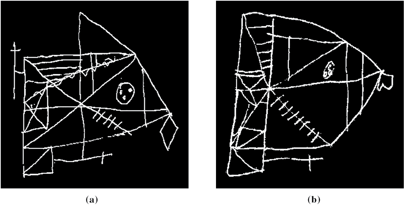
Figure 1: ROCF drawings from the ROCFD528 dataset, drawn by individuals with different cognitive states. (a) Healthy; (b) MCI

Offline Data Augmentation

Our dataset is augmented for two reasons: to have the same number of healthy and MCI figures, preventing the models from having a bias towards the majority class, and to increase the diversity of the figures, which improves the generalization ability of the models. In this article, we apply offline data augmentation to generate a single augmented dataset, which will be used to evaluate all the models. This dataset includes a training partition, on which augmentation operations are applied, and validation and test partitions, which only contain original images. The generation process starts with the 528 available ROCF drawings. From these, we separate 32 samples (16 healthy, 16 MCI) for the test partition. For the remaining 496 ROCF drawings (300 healthy, 196 MCI), we will apply a CV scheme ensuring class balance in each of the folds. To achieve this, we separate 104 healthy ROCF drawings, and the remaining 392 ROCF drawings (196 healthy, 196 MCI) are divided into 14 equal parts. In each CV iteration, one part (14 healthy, 14 MCI) will be used to validate the model and 13 parts to train it (182 healthy, 182 MCI). On these training parts and the 104 healthy ROCF drawings that we previously separated, data augmentation is applied until reaching 1200 ROCF drawings (600 healthy, 600 MCI). To achieve this number, we generate 314 new healthy ROCF drawings and 418 new MCI drawings by applying transformations to their respective counterparts within the training partition (286 healthy, 182 MCI). These transformations are slight rotations (up to 8 degrees), shears (up to 12 degrees), and scaling (with factors ranging from 0.98 to 1.15). The combination of the augmented training partition and the drawings used for model validation and testing represents the final augmented dataset, which we refer to as ROCF Augmented Dataset 1260 (ROCFAD1260). Fig. 2 provides a visual overview of the ROCFAD1260 generation process.

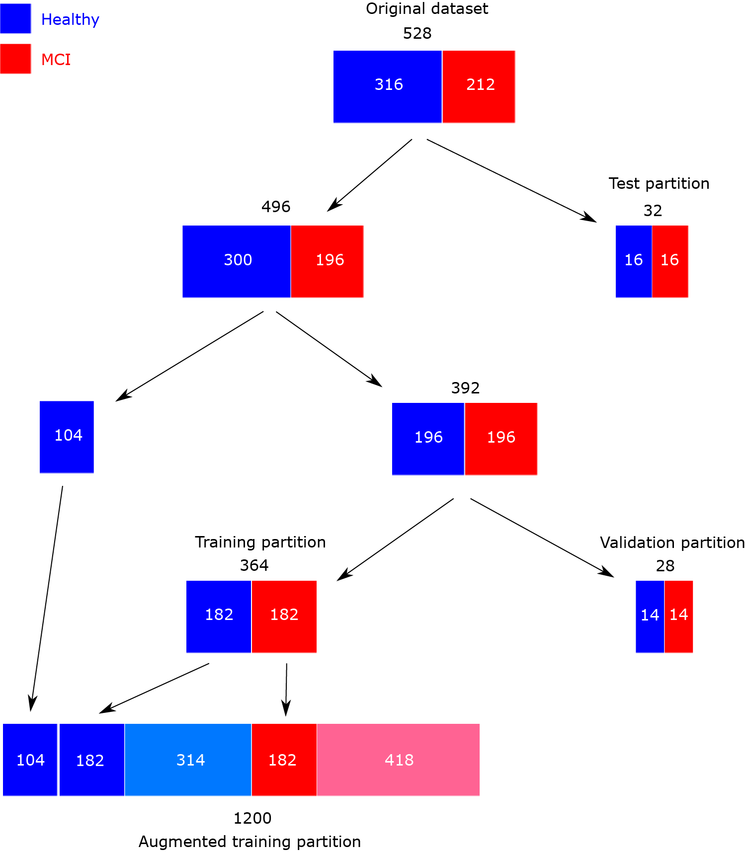
Figure 2: Scheme of ROCF Augmented Dataset 1260 generation

3.2 Siamese Neural Network Proposal

The original SNN architecture [30] consists of two identical neural networks that are responsible for extracting a feature vector or embedding from each element of the input pair. During training, the distance between embeddings guides the formation of a latent space where elements belonging to the same class are close. After training is completed, in the inference stage, the embedding of an unseen element is used to determine its class.

Our implementation of the SNN architecture, called Contrastive Loss Siamese Sketch-a-Net (CL-SSaN), utilizes Sketch-a-Net (SaN) [42] for its branches. This choice was driven by the outstanding results of SaN in automatic ROCF scoring [22]. The training process is guided by the contrastive loss function [43,44], which is formulated as follows:

L⁡(a,b,y)=y∗D⁡(a,b)+(1−y)∗m⁢a⁢x⁡(m−D⁡(a,b),0)(1)

where is the embedding of the first image of a pair (or image A), is the embedding of the second image (or image B), is a label associated with the image pair (1 if the classes of the images match; 0 otherwise), D represents the distance between embeddings, and is a margin that pushes embeddings of different classes apart. Fig. 3 shows an illustration of the CL-SSaN architecture.

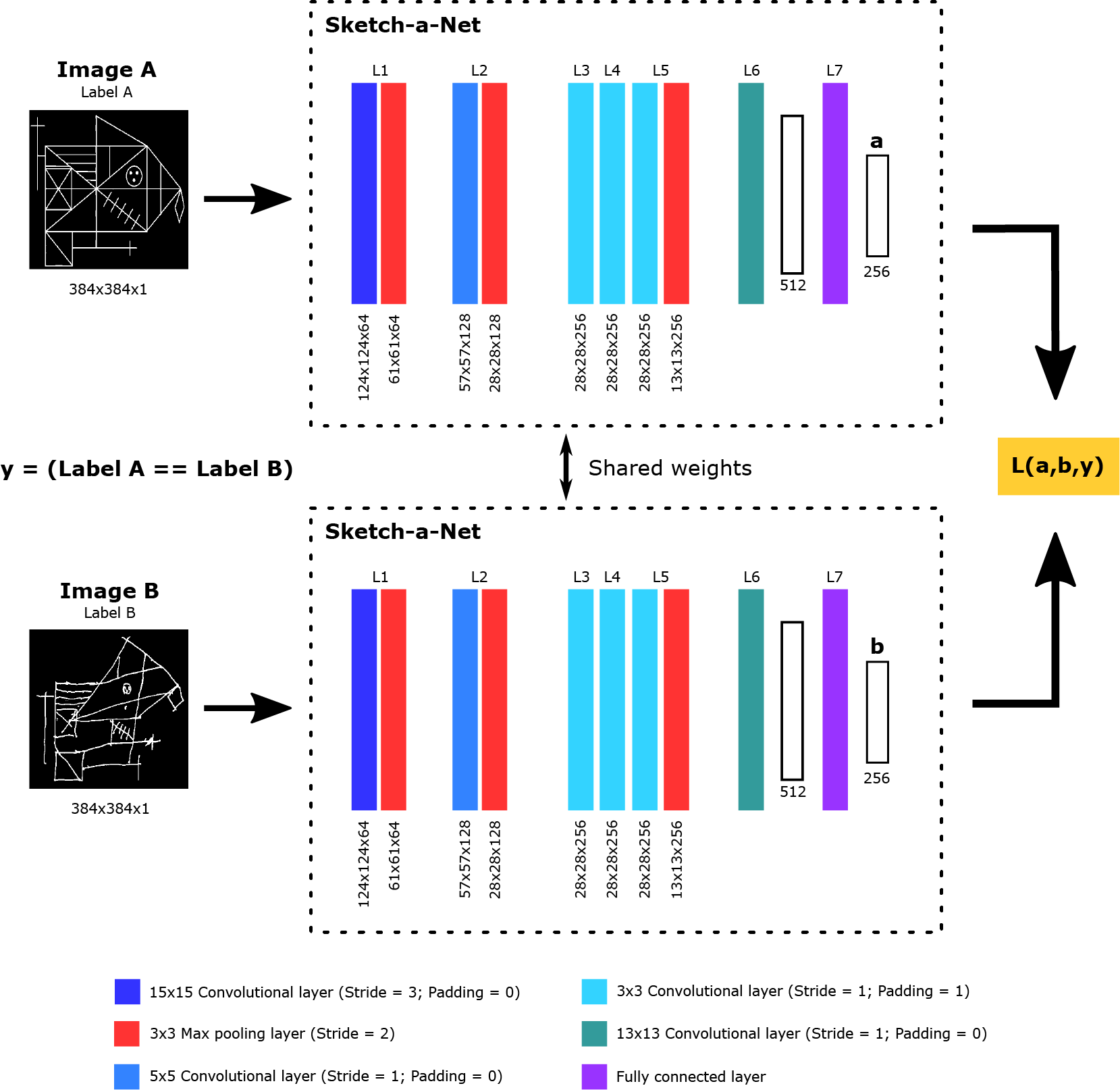
Figure 3: Overview of the CL-SSaN architecture

To train CL-SSaN, image pairs are used such that image A is the ROCF model and image B is each of the 1200 ROCF drawings from the training set. Thus, if image B is labeled as healthy, as assumed for the ROCF model, the pair label will be 1, and if image B is labeled as MCI, will take the value of 0. In this way, Eq. (1) will lead to the generation of a latent space where the embeddings of ROCF drawings labeled as healthy are close to the ROCF model embedding, and the embeddings of ROCF drawings labeled as MCI are as far apart as possible.

In the inference stage, the embedding of any given ROCF and its distance to the ROCF model will help decide whether it is an ROCF drawn by a healthy or MCI-diagnosed individual. The utilization of the ROCF model as a representative of the ROCF drawings labeled as healthy facilitates the definition of the two ROCF groups in the latent space.

4  Results and Discussion

To verify the performance of CL-SSaN, it is compared with that of several DL architectures. In Section 4.1, we compare CL-SSaN with its individual equivalent, a SaN, to analyze the impact of framing the task of predicting an individual’s cognitive state as a distance metric learning problem. On the other hand, in Section 4.2, we compare CL-SSaN with the three state-of-the-art DL-based architectures using the ROCFAD1260 dataset, to see if our proposal offers better results under equivalent conditions. In Section 4.3, we conduct all these performance comparisons using a non-augmented version of the ROCFAD1260 dataset so that we can understand the effects driven by the additional images. Besides comparing the performance of the models, in Section 4.4, we analyze their classification logic for ROCF drawings using an explainable artificial intelligence (XAI) [45] technique to identify potential biases. Finally, in Section 4.5, we study the size and computational cost of the models in relation to their performance to pinpoint areas for optimization prior to deployment.

4.1 Comparison of CL-SSaN Performance with Its Individual Equivalent

In this first experiment, we compare our SNN proposal formed by two SaNs with its individual equivalent, which would be a single SaN. By doing this, we compare the performance of a model designed to solve a distance metric learning problem with a model intended to solve a classification problem, regardless of the network architecture. For both the individual SaN and the two SaNs that form CL-SSaN, we make a slight modification to the original architecture presented in [42], reducing the number of L7 units from 512 to 256 (this will be the size of the image embeddings, as shown in Fig. 3). We made that decision because 512 units seemed excessive for our scenario. The final value of 256 was established after comparing the results obtained with 512, 256 and 128 units. Regarding the contrastive loss function (Eq. (1)), we opt to use cosine distance with a margin of 5e−5. Our selection of this distance function is motivated by its direct proportionality to an L2-normalization of the squared Euclidean distance. This normalization ensures that the difference between two vectors is determined solely by their direction, avoiding problems associated with their magnitude in high dimensions. We corroborated the benefits of cosine distance by comparing CL-SSaN performance when using it against squared Euclidean distance. For the margin, we determined its optimum (5e−5) by testing different values ranging from 5e−6 to 5e−4. Continuing with the CL-SSaN configuration, we have discovered that removing the dropout layers in L6 and L7 [42] leads to better performance. While dropout forces individual neural networks to explore diverse pathways for enhanced generalization, in an SNN with multiple branches and shared weights, we have noticed that the introduced randomness leads to pronounced alterations in the comparison of image pairs, thereby negatively impacting the formation of the latent space.

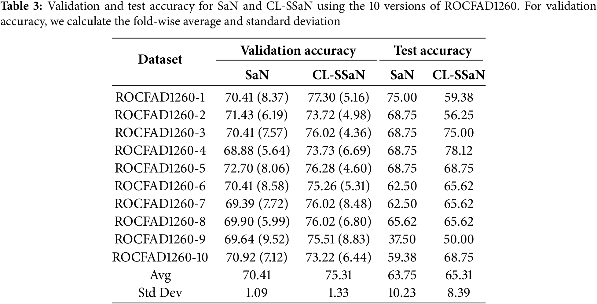
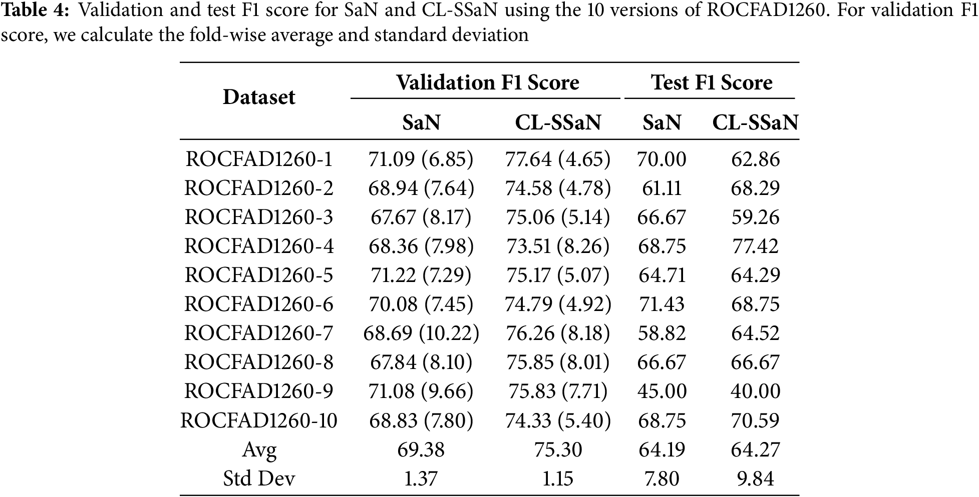
To train and evaluate the two architectures, SaN and CL-SSaN, we use 10 versions of the ROCFAD1260 dataset, labeled from 1 to 10. These versions are generated by modifying the random seeds that define the ROCF drawings belonging to each of the dataset partitions. The following hyperparameters are used to train the architectures: a batch size of 32, a learning rate of 1e−4, and an Adam optimizer with Keras default parameters. The number of training epochs varies, with 250 for SaN and 100 for CL-SSaN. The loss function used for SaN is binary cross-entropy and contrastive (Eq. (1)) for CL-SSaN. When training is completed, for each of the 14 validation folds, the model corresponding to the minimum validation loss is retained. Next, for each model, we choose the probability (SaN) or distance (CL-SSaN) threshold that maximizes validation accuracy, on the one hand, and validation F1 score, on the other. The resulting 14 values are then averaged to obtain the aggregate validation accuracy and F1 score. To calculate the test accuracy and F1 score, we employ the model whose validation metric is the closest to the fold-wise average. For the threshold, we perform an exhaustive search to find the candidate that maximizes the fold-wise micro-averaged accuracy or F1 score.

Table 3 shows the validation and test accuracy for SaN and CL-SSaN. For the validation accuracy, we show the fold-wise average and standard deviation. The values of the metrics are extracted for each version of ROCFAD1260 and, at the end of the table, the global average and standard deviation are shown. Table 4 shows the corresponding F1 scores. If we look at the global averages, it can be seen that CL-SSaN clearly outperforms SaN for both validation accuracy and F1 score, highlighting the potential of our proposal. In contrast, for test accuracy and F1 score, the global averages are very similar. To statistically confirm this similarity, we compare the ten values obtained for the two models using Mann-Whitney U test. The p-values of 1 for accuracy and 0.909 for F1 score indicate that there is no evidence to conclude that there is a significant difference between the two sets of values. However, we would like to emphasize the superiority of our proposal in six versions of ROCFAD1260 for test accuracy and four versions of ROCFAD1260 for test F1 score. This positions CL-SSaN as a valuable alternative for discriminating between ROCF drawings when its individual equivalent exhibits poor performance.

4.2 Comparison of CL-SSaN Performance with State-Of-the-Art Architectures

In this second experiment, we aim to compare the performance of CL-SSaN with that of the three DL architectures mentioned in Section 2, which were designed to classify an ROCF drawing in terms of the individual’s cognitive state: Convolutional Autoencoder + Multilayer Perceptron (CAE + MLP) [35], Youn’s Convolutional Neural Network (YCNN) [36], and Park’s Convolutional Neural Network (PCNN) [37]. The configuration of the YCNN and PCNN architectures is the same as that proposed by their authors: five convolutional layers and one dense layer with sizes 64-64-64-64-128 and 128, and four convolutional layers and two dense layers with sizes 32-32-32-32 and 256-128, respectively. However, the configuration of the CAE + MLP architecture is adapted to the characteristics of our images. For the CAE part, we modify the convolutional layers of the encoder and decoder to have sizes 128-64-32-16 and 16-32-64-128, respectively. These changes result in an input size of 9216 for the MLP part, to which we assign two dense layers of size 2048-512.

To train and evaluate the state-of-the-art architectures, we use five versions of ROCFAD1260 defined in Section 4.1: ROCFAD1260-1, ROCFAD1260-3, ROCFAD1260-4, ROCFAD1260-6, and ROCFAD1260-10. We work with these versions to reduce computation time. The selection criterion is based on the validation accuracy value obtained for CL-SSaN (Table 3). With ROCFAD1260-6, ROCFAD1260-4, and ROCFAD1260-3, we obtain the value closest to the average (75.26%), one half of a standard deviation below (73.73%), and one half of a standard deviation above (76.02%), respectively. We also use the versions corresponding to extreme values: ROCFAD1260-10, associated with the lowest validation accuracy value (73.22%), and ROCFAD1260-1, related to the highest value (77.30%). We want to highlight that the normality of the validation accuracy values is verified using the Anderson-Darling (0.523 given a critical value of 0.684 for a 5% confidence level) and Shapiro-Wilk (0.905 with a p-value of 0.249) tests. For training the architectures, the common hyperparameters are a batch size of 32, a learning rate of 1e−3, and an Adam optimizer with Keras default parameters. The hyperparameter that changes is the number of training epochs, with 1200 for CAE and 100 for MLP, YCNN, and PCNN. The loss function used for the four networks is binary cross-entropy. Once training is completed, the steps to follow are equivalent to those used for SaN.

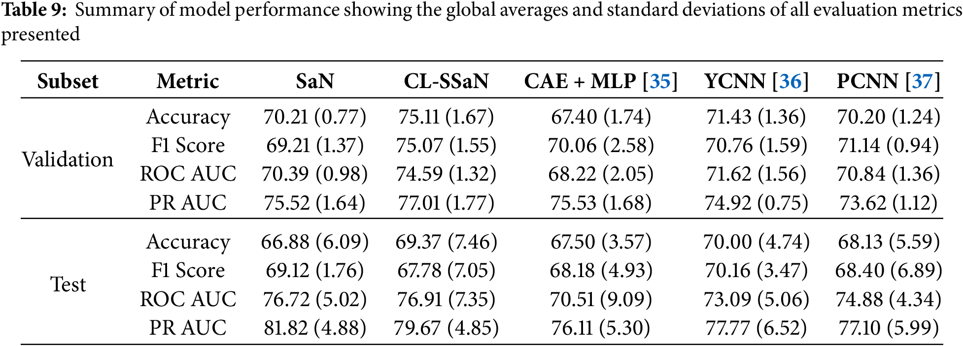
Tables 5 and 6 show the accuracy and F1 score for SaN, CL-SSaN, CAE + MLP [35], YCNN [36], and PCNN [37]. In addition to these metrics, we also calculate the ROC AUC (Table 7) and PR AUC (Table 8), which are independent of the chosen probability (SaN, CAE + MLP, YCNN, and PCNN) and distance (CL-SSaN) thresholds. Fig. 4 shows average validation and test ROC curves, and Fig. 5 displays the corresponding PR curves. Table 9 shows a summary of the global averages and standard deviations for accuracy, F1 score, ROC AUC, and PR AUC of all five models. This table provides a valuable overview of the strengths provided by each model. If we analyze it, we can observe that CL-SSaN achieves the best values for all validation metrics with a clear difference from its competitors. It is worth noting that for PR AUC the differences are smaller, underscoring the challenge of detecting and predicting ROCF drawings produced by individuals with MCI. Focusing now on the test metric values, we want to state that the performance differences between models cannot be considered significant, given the number of evaluation rounds and the high standard deviations. Nevertheless, analyzing these differences is important, as it allows us to understand the subtle advantages of some models over others. While YCNN achieves the best accuracy and F1 score (followed closely by CL-SSaN and SaN, respectively), CL-SSaN and SaN show better performance in ROC AUC and PR AUC compared to the three state-of-the-art models. Specifically, CL-SSaN slightly excels in ROC AUC, while SaN achieves a particularly high PR AUC value, reflecting the flexibility of these two models in discriminating between ROCF drawings across different thresholds, a capability that is valuable in real-world deployment.

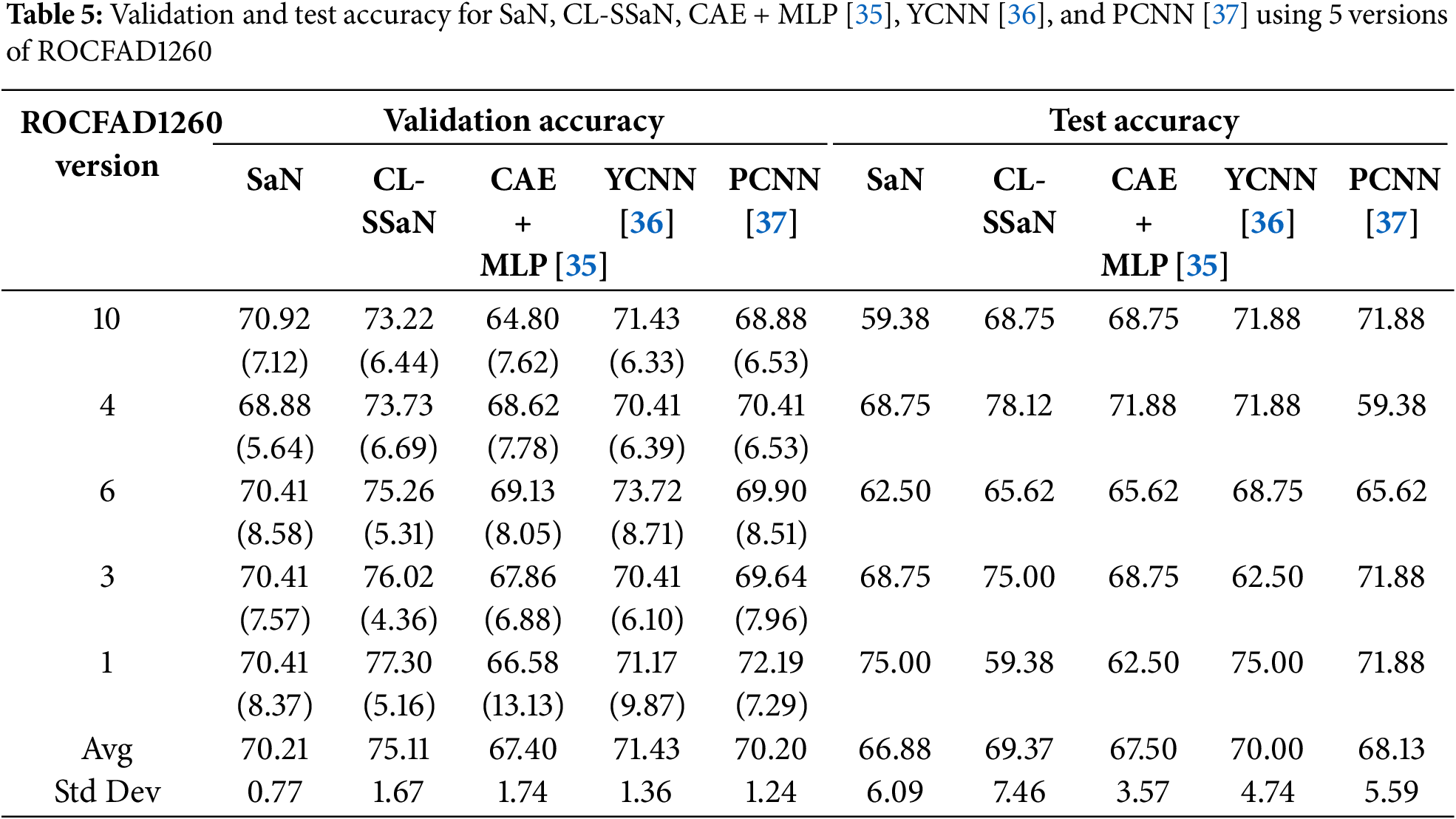
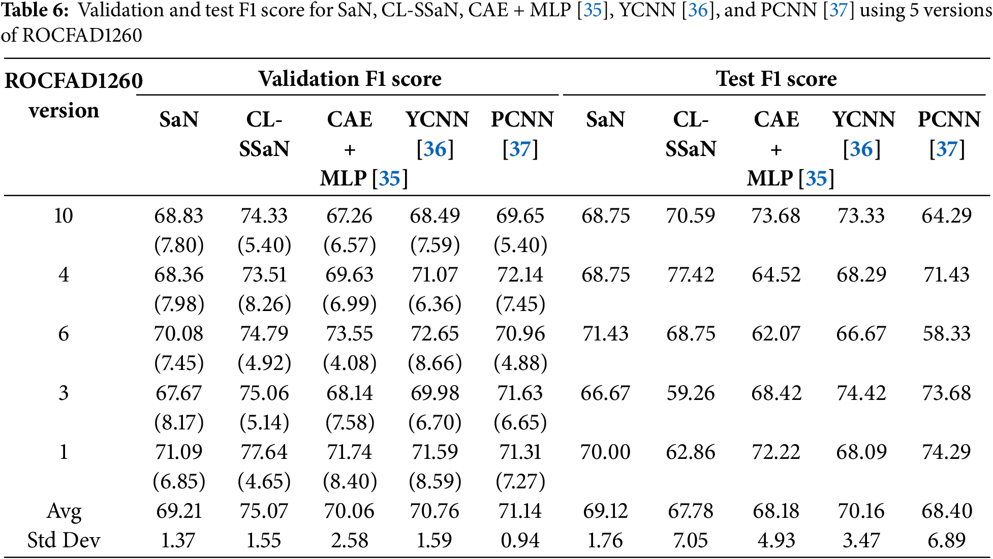
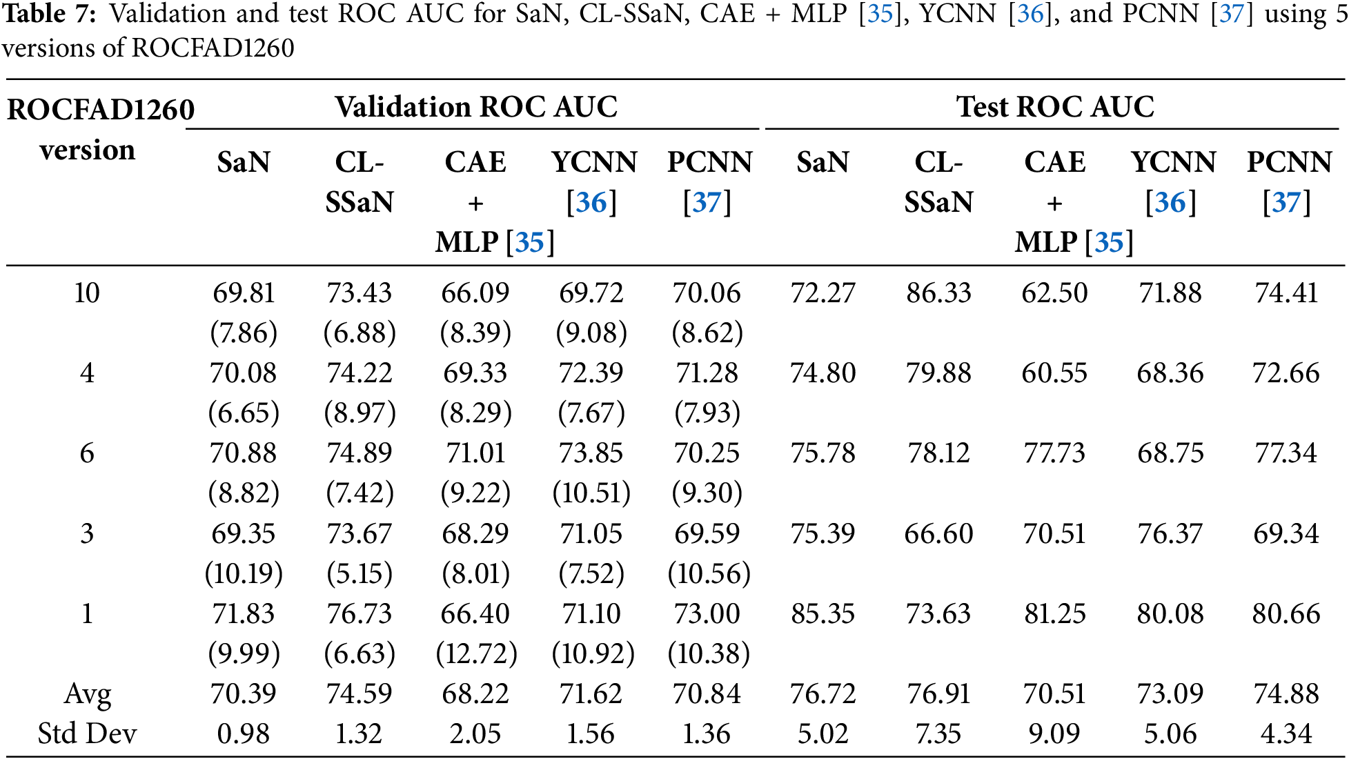
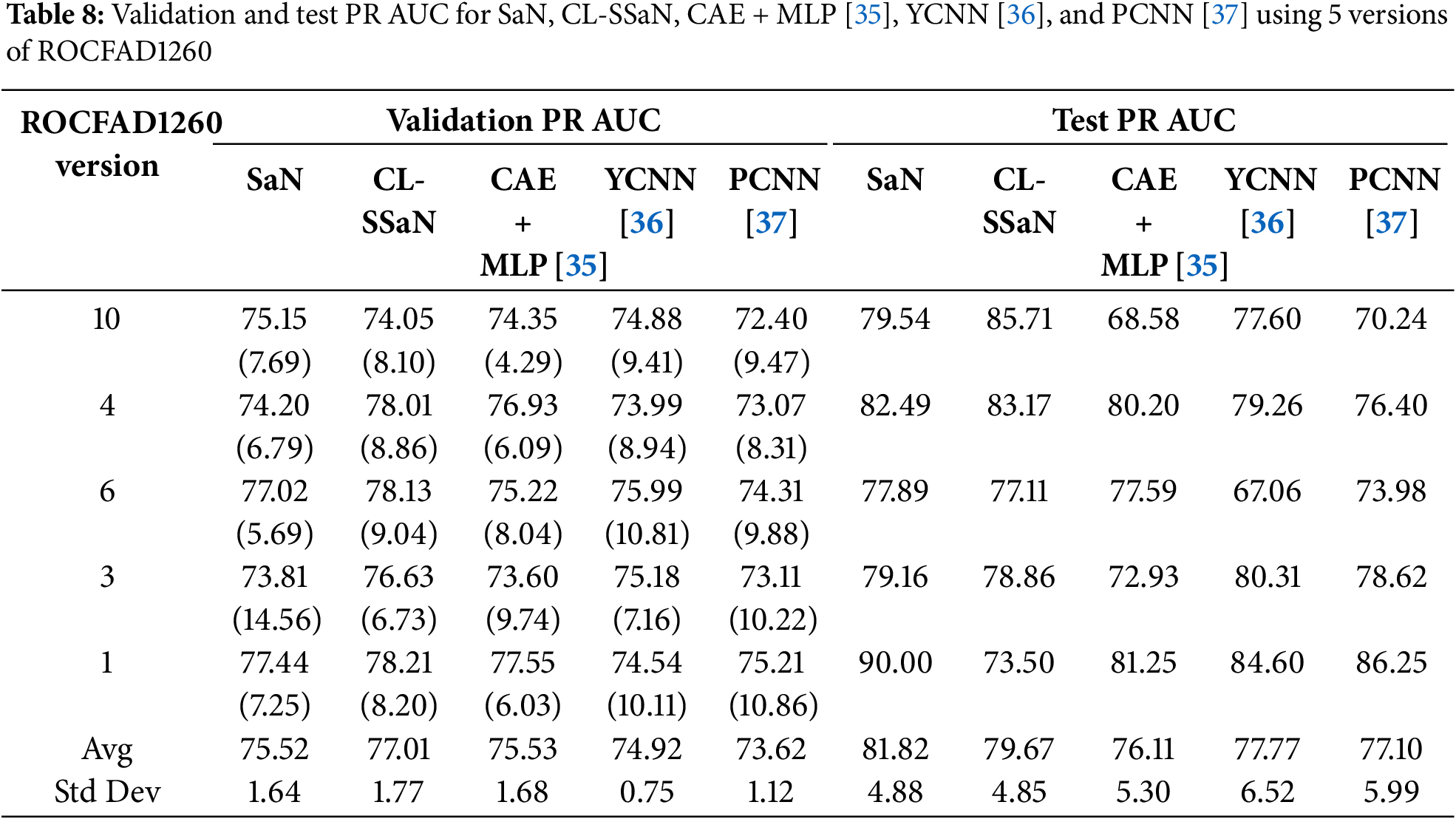
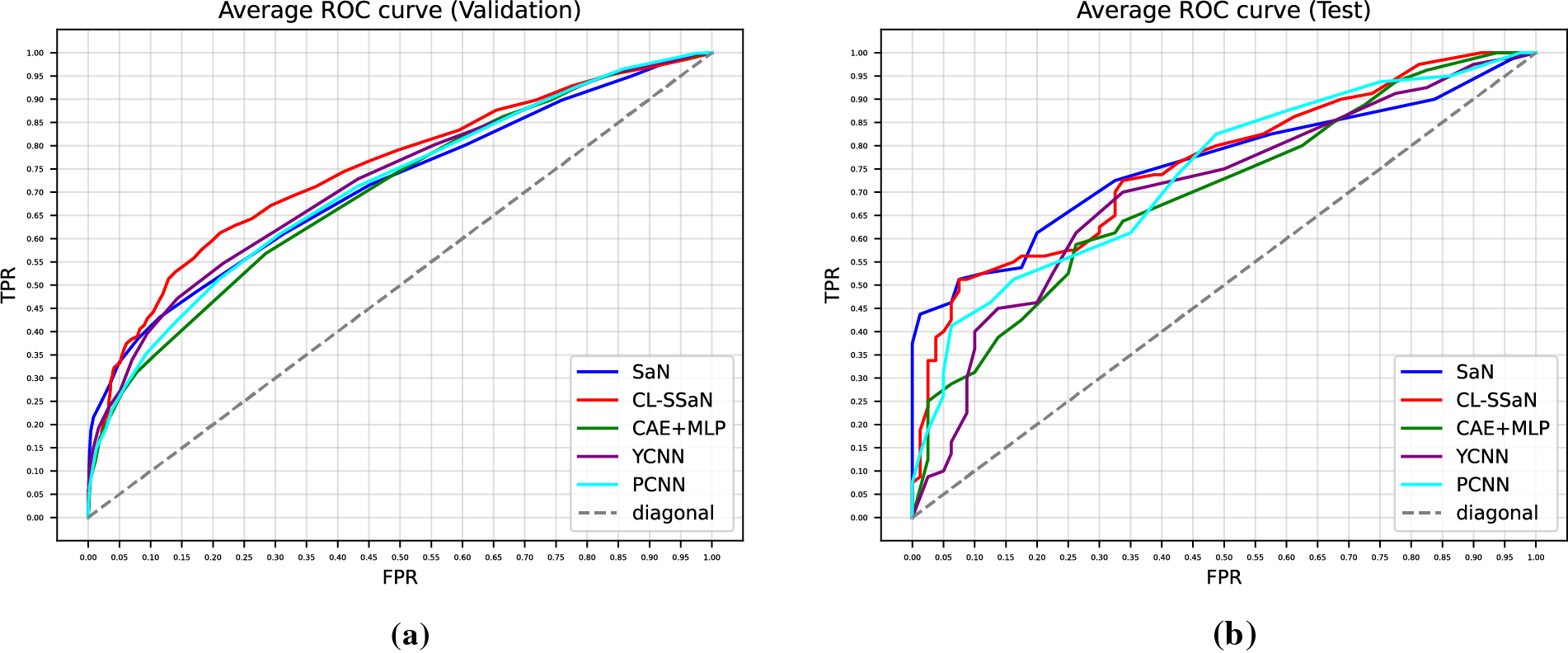
Figure 4: Average ROC curves extracted for SaN, CL-SSaN, CAE + MLP [35], YCNN [36], and PCNN [37]. (a) Corresponding to the validation sets of the five versions of ROCFAD1260; (b) Corresponding to the test sets of the five versions of ROCFAD1260

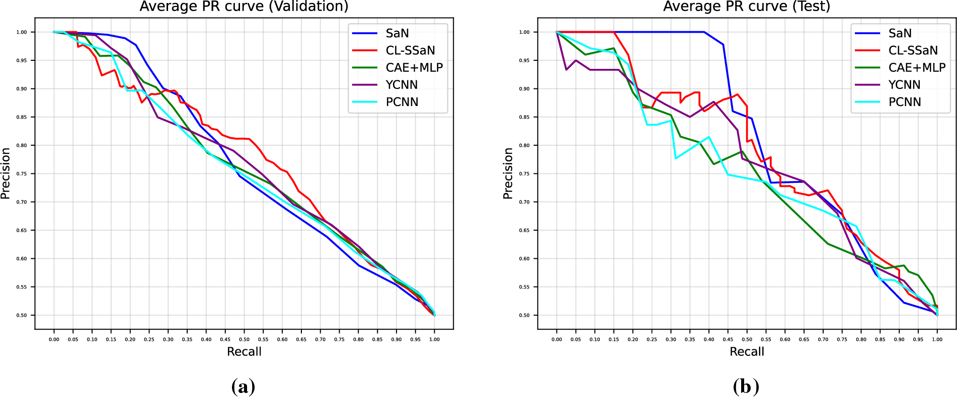
Figure 5: Average PR curves extracted for SaN, CL-SSaN, CAE + MLP [35], YCNN [36], and PCNN [37]. (a) Corresponding to the validation sets of the five versions of ROCFAD1260; (b) Corresponding to the test sets of the five versions of ROCFAD1260

4.3 Model Performance Using the Non-Augmented Dataset

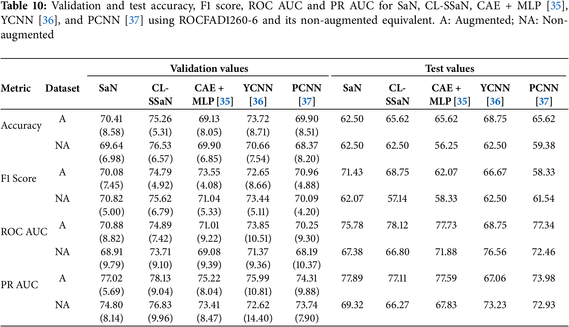
All results shown in the two previous sections are achieved by training the models with 1200 ROCF drawings (Fig. 2). Of these drawings, 468 are original versions, and the remaining 732 are augmented versions. In this section, we analyze what would happen if we trained all models exclusively with the original drawings. Specifically, we utilize version 6 of ROCFAD1260 (the one with validation accuracy closest to the average), remove the augmented drawings from its training set, and train all five models. Table 10 shows a comparison of the accuracy, F1 score, ROC AUC, and PR AUC obtained using the original definition of ROCFAD1260-6 and its non-augmented version. Observing the validation accuracy and F1 score values, we cannot say that data augmentation has led to significant changes. However, if we look at the threshold-independent metrics (validation ROC AUC and PR AUC), it can be appreciated that the additional images provide a consistent improvement for all models. Furthermore, these improvements do not appear to be significantly better for ROC AUC than for PR AUC, or vice versa. Regarding the test results, we can observe a consistent improvement for the models trained with the augmented dataset, which suggests that data augmentation is successfully reducing overfitting. The only exceptions are SaN for accuracy, PCNN for F1 score, and YCNN for ROC AUC and PR AUC. The first two cases can be explained by the particularly low results of SaN (Table 5) and PCNN (Table 6) in relation to the other ROCFAD1260 versions, which implies that the margin for improvement with data augmentation is limited. Meanwhile, the case concerning YCNN is explained by the models selected for obtaining the test metric values, which were those with validation ROC AUC and PR AUC values closest to the average. If, instead of these models, we choose those closest to the average validation accuracy and F1 score and calculate the test ROC AUC and PR AUC, respectively, we obtain 71.09 and 67.38 for ROC AUC, and 75.86 and 69.69 for PR AUC. These alternative values are clearly aligned with those obtained for the other four models.

4.4 Model Interpretability

The quantitative results presented in Sections 4.1–4.3 give us an idea of the performance each model will have in a deployment environment. However, these results do not reveal the logic followed by each model to assign the healthy or MCI class to the ROCF drawings in the test set. To gain understanding of this logic, we apply an XAI technique designed for CNN-based models called Gradient-weighted Class Activation Mapping (Grad-CAM) [46]. This technique generates a heatmap for a given input image that highlights the regions with a greater influence on the model output. The regions are estimated using the gradients that flow from the model output to any of the model convolutional layers. The models we apply Grad-CAM to are the ones used to calculate the test accuracy (Table 5). We focus on SaN, CL-SSaN, and YCNN, and on ROCFAD1260 versions 1, 4 and 6. We choose YCNN as it is the state-of-the-art model with the best test accuracy and F1 score (Table 9) and opt for versions 1, 4, and 6 as they represent scenarios where CL-SSaN performance is inferior, superior, and similar to that of the other models, respectively. Additionally, we also apply Grad-CAM to the three models trained with the non-augmented version of ROCFAD1200-6, to visually understand the effects of data augmentation.

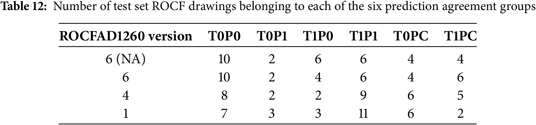
For each model, we generate Grad-CAM heatmaps for all 32 ROCF drawings in the test set. Before showing some of these heatmaps, we want to provide adequate context for the test set drawings by detailing their true and predicted labels. The drawings are organized in two ways: first, via confusion matrices for each model, and second, by categorizing them into six distinct groups based on their true labels and the predictions from the three models. These six groups are: T0P0 (true healthy, predicted healthy), T1P1 (true MCI, predicted MCI), T0P1 (true healthy, predicted MCI), T1P0 (true MCI, predicted healthy), T0PC (true healthy, conflicting predictions), and T1PC (true MCI, conflicting predictions). Table 11 shows the confusion matrices, and Table 12 shows the distribution of drawings based on the prediction agreement groups. If we analyze the ROCFAD1260-6 confusion matrices, we can appreciate how data augmentation enables CL-SSaN to identify three additional MCI drawings (at the cost of misidentifying two healthy ones), allows YCNN to find two more healthy drawings, and has no effect on SaN, which mantains its low TP count. Analyzing the ROCFAD1260-4 confusion matrices, we see that CL-SSaN is able to detect a high number of MCI drawings without sacrificing TNs. Conversely, SaN and YCNN must trade off detection rates between classes. Finally, regarding the ROCFAD1260-1 confusion matrices, it is CL-SSaN that identifies a relatively low number of healthy drawings. If we now look at Table 12, we can find some connections with Table 11. For ROCFAD1260-6, we can observe that all the TPs obtained by SaN are from the T1P1 group, and only CL-SSaN and YCNN are capable of detecting MCI drawings where there is a conflict (group T1PC). For ROCFAD1260-4, the number of T0P0 and T1P1 drawings is high, while the number of T0P1 and T1P0 drawings is low. In this scenario, CL-SSaN is capable of achieving a high number of both TNs and TPs. Finally, for ROCFAD1260-1, CL-SSaN can only detect one healthy drawing from the T0PC group. The visualization of Grad-CAM heatmaps for drawings belonging to each prediction agreement group will allow us to better interpret the behavior of each model.

Figs. 6 and 7 show Grad-CAM heatmaps obtained for test set ROCF drawings. For each drawing, we generate four heatmaps corresponding to convolutional layers 1, 2, 4, and 5 (L1, L2, L4, and L5 in Fig. 3), displayed from left to right and top to bottom. The heatmaps use a color scale from blue to red, indicating a decrease and increase, respectively, in the model output. This output corresponds to the MCI probability for SaN and YCNN, and the distance to the ROCF model for CL-SSaN. Fig. 6 shows heatmaps for two drawings belonging to ROCFAD1260-6 test set whose predictions improve with data augmentation. In Fig. 6a, CL-SSaN correctly predicts the drawing as MCI by emphasizing the interior regions of the figure, while in Fig. 6b, YCNN correctly labels the drawing as healthy due to a pronounced focus on the figure border. Fig. 7 shows the heatmaps generated for several drawings belonging to the six prediction agreement groups. In Fig. 7a, we see a drawing from the T0P0 group. These ROCF drawings closely resemble the ideal ROCF, and the models consistently predict their labels. However, the decision-making logic followed by each model differs: SaN focuses on the drawing general shape and internal areas that may be distorted (see the last heatmap), CL-SSaN inherits SaN behavior, but it is mainly guided by the distance to the ROCF model (as inferred from the predominance of blue in the four heatmaps), and YCNN seems to prioritize strokes, likely due to its convolutional kernel sizes. Fig. 7b shows a T1P1 drawing. Here, SaN late layers find irregular areas that are inconsistent with the ROCF model, while CL-SSaN and YCNN detect anomalies in the stroke shapes. Fig. 7c shows a drawing labeled as healthy but predicted as MCI by all models. We have observed that this normally occurs when the drawing is similar to the ROCF model but its size is small or it has pronounced (especially negative) shearing. In Fig. 7d, we have the opposite scenario, where the drawing is labeled as MCI but all three models consider it healthy. This generally happens when the drawing strongly resembles the ROCF model, yet the individual was diagnosed with MCI based on the results of other neuropsychological tests. Fig. 7e–g shows drawings corresponding to the most frequent T0PC scenarios. In Fig. 7e, YCNN likely fails because it is too sensitive to stroke noise, like changes in curvature or thickness. In Fig. 7f, SaN correctly labels the drawing because it disregards the excessive noise in the center (due to its broader focus). Lastly, in Fig. 7g, CL-SSaN likely mislabels the drawing due to scan noise and the scaling issue mentioned for Fig. 7c. We finalize the heatmap analysis with the drawings shown in Fig. 7h–j, which correspond to the most frequent T1PC scenarios. In these scenarios, SaN wrongly labels the drawing as healthy because it recognizes several components of the figure, even though these are quite misplaced and distorted. These alterations are successfully detected by the middle layers (see second and third heatmaps) of CL-SSaN and YCNN, leading to a correct MCI prediction.

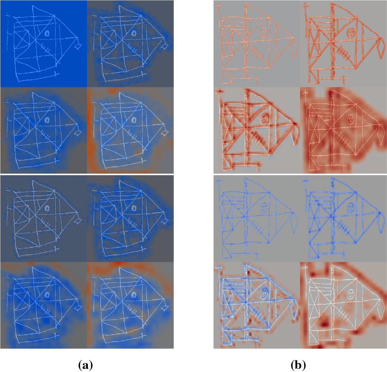
Figure 6: Comparison of Grad-CAM heatmaps of drawings processed by models trained using non-augmented ROCFAD1260-6 (top row) and ROCFAD1260-6 (bottom row). We show four heatmaps corresponding to convolutional layers 1, 2, 4, and 5, from left to right and top to bottom. (a) Drawing with true label 1 processed by CL-SSaN (the predicted label changes from 0 to 1); (b) Drawing with true label 0 processed by YCNN (the predicted label changes from 1 to 0)

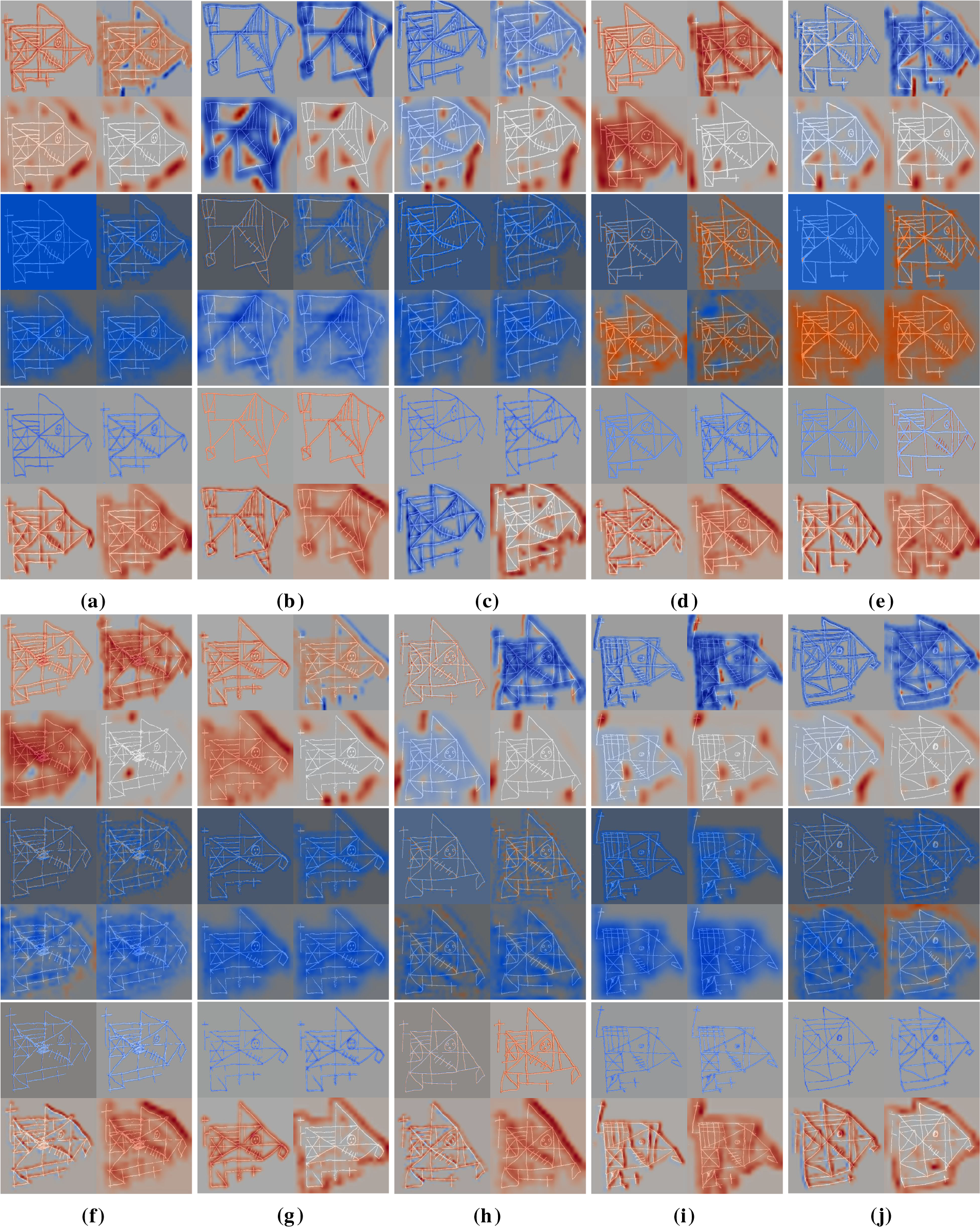
Figure 7: Grad-CAM heatmaps obtained for drawings belonging to the six prediction agreement groups. We show four heatmaps corresponding to convolutional layers 1, 2, 4, and 5, from left to right and top to bottom. For each drawing, we show the heatmaps obtained for SaN, CL-SSaN and YCNN, from top to bottom. (a) T0P0; (b) T1P1; (c) T0P1; (d) T1P0; (e) T0 P001 (YCNN misclassifies); (f) T0 P011 (SaN is the only one that is correct); (g) T0 P010 (CL-SSaN misclassifies); (h) T1 P001 (YCNN is the only one that is correct); (i) T1 P011 (SaN misclassifies); (j) T1 P010 (CL-SSaN is the only one that is correct)

Gathering the knowledge extracted from the analyzed Grad-CAM heatmaps, we can derive a series of key points to understand the performance of each model. We have observed that SaN usually labels the highest number of healthy drawings correctly (Table 11), primarily due to its focus on the overall structure of the figure. However, this broader focus might also be the main contributor to the low number of correctly predicted MCI drawings. Regarding CL-SSaN and YCNN, we have found that the distance criterion of the former and the focus on strokes of the latter are critical for detecting certain MCI ROCF drawings. This contributes to a high number of true positives and a reduced number of false negatives, which is desirable in a clinical context. On a negative note, CL-SSaN and YCNN sometimes misclassify healthy drawings. This is occasionally explained by their architectures, but at times it is related to scan noise or certain image transformations. We intend to analyze these latter cases in detail.

4.5 Model Computational Cost and Size Analysis

To anticipate the behavior of the five analyzed models in a production or deployment environment, we extract their number of parameters and the number of floating-point (FP) operations required to process a single ROCF drawing (we use the TensorFlow profiler to calculate this number). Model test accuracy is added to the comparison to analyze possible trade-offs. Fig. 8a shows the relationship between test accuracy and giga FP operations for all five models, while Fig. 8b displays the test accuracy against the number of parameters. The first thing we would like to highlight about these plots is how CL-SSaN offers a slightly higher test accuracy using the same number of parameters and FP operations as its individual equivalent. This happens because SNNs share weights between branches, and therefore, only one of them is needed for the inference stage. Focusing now on Fig. 8a, we can see that the computational cost of CAE + MLP is very low compared to that of the other models, as only the MLP part is used for inference. But, we should keep in mind that the training computational cost would be significantly high. If we look at CL-SSaN, we can notice that it offers an accuracy-computational cost relationship very close to that of YCNN. In Fig. 8b, the roles of CAE + MLP and YCNN are swapped. The MLP has a very high number of parameters due to its fully connected layers, while YCNN has the lowest number of parameters because its design is almost exclusively composed of convolutional layers. Finally, PCNN shows reduced computational cost and size, making it an attractive option for potential deployment. Combining the characteristics of this architecture with those of SaN could be a good optimization exercise. The resulting network could then be transformed into an SNN, given the alternative it offers for discriminating certain drawings without increasing the number of parameters or FP operations.

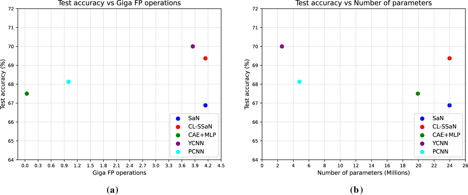
Figure 8: Comparison of model test accuracy with its computational cost and size. (a) Model test accuracy vs. giga floating-point (FP) operations; (b) Model test accuracy vs. number of parameters

5  Limitations and Future Directions

The main limitation we face is the reduced availability of real data. If we had a significantly larger number of images, we could check whether distance metric learning models outperform classification models, or if, on the contrary, the former are only comparable when data is scarce. In addition to having more ROCF drawings in general, it would be especially interesting to have access to ROCF drawings made from memory to train our SNN proposal. Two of the studies presented in Section 2 report results for healthy-MCI classification using this type of ROCF drawing. Concretely, Cheah et al. [35] obtain a sensitivity of 0.712 using copy drawings and 0.756 using delayed recall drawings, while Park [37] report sensitivity values of 0.843 and 0.864, respectively. A relevant future work would be to check if these differences are maintained using our model, a large dataset of delayed recall ROCF drawings, and an exhaustive evaluation protocol.

Besides collecting new drawings, we would like to apply a series of improvements to the ROCFD528 dataset. On the one hand, we want to process all drawings in the dataset to reduce or eliminate scan noise. This action would allow for the reduction of false positives in models particularly sensitive to stroke noise, such as CL-SSaN or YCNN. On the other hand, we aim to have a discussion with the psychologists we collaborate with to understand if certain scaling or shearing transformations of a drawing could be related to MCI. If this theory is rejected, we would work on improving the data augmentation process, creating more augmented images and strategically selecting the transformations. This way, the models would only focus on the interior of the figure to classify it.

Apart from working on the data, we would also explore different approaches in the design and training of SNNs that could lead to better results: using other architectures in the SNN branches that place a greater emphasis on the ROCF drawing strokes, ensuring that these architectures entail a low number of parameters and FP operations, modifying the loss function, implementing regularization techniques alternative to dropout (to mitigate potential overfitting), applying online data augmentation and pair generation, creating pairs omitting the ROCF model, using pair selection techniques, defining criteria for grouping elements in the latent space, etc. All these ideas could be applied to siamese pair neural networks, but we also want to highlight the possibility of using triplet neural networks, such as those described in [47]. As their name suggests, the input to the network is three images, of which one acts as an anchor, another is of the same class as the anchor, and the last is of a different class from the anchor. The simultaneous comparison of the anchor with the other two images could lead to even better discrimination between ROCFs drawn by individuals with different cognitive states. However, handling this type of network implies a series of challenges related to the combinatorial complexity and redundancy inherent in triplets.

After applying these improvements to the data and to our SNN proposal, we could consider its deployment in a real clinical environment. In this scenario, we would optimize our model to obtain the maximum F1 score, perhaps giving a more pronounced weight to recall (we are interested in minimizing the number of MCI drawings that are incorrectly predicted as healthy). If the model were to predict an individual’s ROCF drawing as MCI, this result could be considered a preliminary screening step before conducting expensive medical tests, such as blood or cerebrospinal fluid analysis or medical imaging. These tests would serve to verify the diagnosis suggested by our model.

6  Conclusion

In this article, we propose a distance metric learning model to provide an early screening of an individual’s cognitive state based on their ROCF copy drawing. Specifically, we use an SNN formed by two SaNs that employs the distance of any ROCF to the ROCF model to determine if the former was drawn by a healthy individual or one with MCI. Our proposal demonstrates comparable performance to four DL-based classification models. Notably, it also achieves high accuracy and F1 scores on some test sets where the other models perform poorly. In addition to its performance, our analysis of the Grad-CAM heatmaps reveals that its distance criterion is a key factor in identifying certain MCI drawings. All of these advantages are valuable in a scenario where we have a very limited number of ROCF drawings, the drawing of the figure by individuals is characterized by its enormous variability, and the relationship between the drawing and the diagnosis is not always direct or intuitive. Beyond offering an alternative for discriminating ROCF drawings, our model also provides benefits for future deployment, given that its inference cost, in terms of number of parameters and floating-point operations, is equivalent to that of a single branch. For future work, we will improve the image quality of our drawings, revise the data augmentation process, and collect new ROCF drawings, including those drawn from memory. Additionally, we will adapt the design of our proposal to better capture the subtle differences between ROCF drawings produced by individuals with varying diagnoses. Once we have implemented these improvements, we will work on integrating our model into a real clinical environment.

Acknowledgement: The authors thank the collaborating psychologists, Sara García-Herranz and María del Carmen Díaz-Mardomingo, for kindly sharing the diagnoses associated with each individual and neuropsychological evaluation session.

Funding Statement: This research has been supported by an FPI-UNED-2021 scholarship.

Author Contributions: The authors confirm contribution to the paper as follows: conceptualization and methodology: Juan Guerrero-Martín, Eladio Estella-Nonay, Margarita Bachiller-Mayoral and Mariano Rincón; data curation, formal analysis, software and draft manuscript preparation: Juan Guerrero-Martín; supervision, project administration and funding acquisition: Margarita Bachiller-Mayoral and Mariano Rincón. All authors reviewed the results and approved the final version of the manuscript.

Availability of Data and Materials: The links to the open code and data can be found on this website: https://edatos.consorciomadrono.es/dataverse/rey (accessed on 23 September 2025). Please note that to access the diagnoses, a formal request is necessary.

Ethics Approval: Not applicable.

Conflicts of Interest: The authors declare no conflicts of interest to report regarding the present study.

References

1. Nichols E, Steinmetz JD, Vollset SE, Fukutaki K, Chalek J, Abd-Allah F, et al. Estimation of the global prevalence of dementia in 2019 and forecasted prevalence in 2050: an analysis for the Global Burden of Disease Study 2019. Lancet Public Health. 2022;7(2):e105–25. doi:10.1016/S2468-2667(21)00249-8. [Google Scholar] [PubMed] [CrossRef]

2. Gauthier S, Reisberg B, Zaudig M, Petersen RC, Ritchie K, Broich K, et al. Mild cognitive impairment. The Lancet. 2006;367(9518):1262–70. doi:10.1016/S0140-6736(06)68542-5. [Google Scholar] [PubMed] [CrossRef]

3. Reuben DB, Kremen S, Maust DT. Dementia prevention and treatment: a narrative review. JAMA Intern Med. 2024;184(5):563–72. doi:10.1001/jamainternmed.2023.8522. [Google Scholar] [PubMed] [CrossRef]

4. Hane FT, Robinson M, Lee BY, Bai O, Leonenko Z, Albert MS. Recent progress in Alzheimer’s disease research, part 3: diagnosis and treatment. J Alzheimer’s Disease. 2017;57(3):645–65. doi:10.3233/JAD-160907. [Google Scholar] [PubMed] [CrossRef]

5. Dickerson BC, Atri A, Clevenger C, Karlawish J, Knopman D, Lin PJ, et al. The Alzheimer’s association clinical practice guideline for the diagnostic evaluation, testing, counseling, and disclosure of suspected Alzheimer’s disease and related disorders (DETeCD-ADRDexecutive summary of recommendations for specialty care. Alzheimer’s Dementia. 2025;21(1):e14337. doi:10.1002/alz.14337. [Google Scholar] [PubMed] [CrossRef]

6. Grueso S, Viejo-Sobera R. Machine learning methods for predicting progression from mild cognitive impairment to Alzheimer’s disease dementia: a systematic review. Alzheimer’s Res Therapy. 2021;13(1):162. doi:10.1186/s13195-021-00900-w. [Google Scholar] [PubMed] [CrossRef]

7. Arya AD, Verma SS, Chakarabarti P, Chakrabarti T, Elngar AA, Kamali AM, et al. A systematic review on machine learning and deep learning techniques in the effective diagnosis of Alzheimer’s disease. Brain Inform. 2023;10(1):17. doi:10.1186/s40708-023-00195-7. [Google Scholar] [PubMed] [CrossRef]

8. Blanco K, Salcidua S, Orellana P, Sauma-Pérez T, León T, Steinmetz LCL, et al. Systematic review: fluid biomarkers and machine learning methods to improve the diagnosis from mild cognitive impairment to Alzheimer’s disease. Alzheimer’s Res Therapy. 2023;15(1):176. doi:10.1186/s13195-023-01304-8. [Google Scholar] [PubMed] [CrossRef]

9. Qiu S, Miller MI, Joshi PS, Lee JC, Xue C, Ni Y, et al. Multimodal deep learning for Alzheimer’s disease dementia assessment. Nat Commun. 2022;13(1):3404. doi:10.1038/s41467-022-31037-5. [Google Scholar] [PubMed] [CrossRef]

10. Grassi M, Rouleaux N, Caldirola D, Loewenstein D, Schruers K, Perna G, et al. A novel ensemble-based machine learning algorithm to predict the conversion from mild cognitive impairment to Alzheimer’s disease using socio-demographic characteristics, clinical information, and neuropsychological measures. Front Neurol. 2019;10(1):756. doi:10.3389/fneur.2019.00756. [Google Scholar] [PubMed] [CrossRef]

11. Mukherji D, Mukherji M, Mukherji N. Alzheimer’s disease neuroimaging initiative. Early detection of Alzheimer’s disease using neuropsychological tests: a predict-diagnose approach using neural networks. Brain Inform. 2022;9(1):23. doi:10.1186/s40708-022-00169-1. [Google Scholar] [PubMed] [CrossRef]

12. Benedet MJ, Alejandre MÁ. TAVEC: test de aprendizaje verbal España-Complutense. Tea Madrid. 1988 [Internet]. [cited 2025 Sep 23]. Available from: https://web.teaediciones.com/tavec-test-de-aprendizaje-verbal-españa-complutense.aspx. [Google Scholar]

13. Delis DC, Kramer JH, Kaplan E, Thompkins BAO. CVLT: California verbal learning test-adult version: manual. Psychological corporation. 1987 [Internet]. [cited 2025 Sep 23]. Available from: https://books.google.es/books?id=0EtIMwEACAAJ. [Google Scholar]

14. Arnett JA, Labovitz SS. Effect of physical layout in performance of the trail making test. Psychol Assess. 1995;7(2):220–1. doi:10.1037/1040-3590.7.2.220. [Google Scholar] [CrossRef]

15. Rey A. L’examen psychologique dans les cas d’encephalopathie traumatique. Archives de Psychologie. 1941;28:215–85. [Google Scholar]

16. Osterrieth PA. Le test de copie d’une figure complexe; contribution a l’etude de la perception et de la memoire. Archives de Psychologie. 1944;30:206–356. [Google Scholar]

17. Shin MS, Park SY, Park SR, Seol SH, Kwon JS. Clinical and empirical applications of the Rey-Osterrieth complex figure test. Nat Protoc. 2006;1(2):892–9. doi:10.1038/nprot.2006.115. [Google Scholar] [PubMed] [CrossRef]

18. Zhang X, Lv L, Min G, Wang Q, Zhao Y, Li Y. Overview of the complex figure test and its clinical application in neuropsychiatric disorders, including copying and recall. Front Neurol. 2021;12:680474. doi:10.3389/fneur.2021.680474. [Google Scholar] [PubMed] [CrossRef]

19. Cummings JL, Benson DF. Dementia of the Alzheimer type: an inventory of diagnostic clinical features. J Am Geriatr Soc. 1986;34(1):12–9. doi:10.1111/j.1532-5415.1986.tb06334.x. [Google Scholar] [PubMed] [CrossRef]

20. Lezak MD, Howieson DB, Bigler ED, Tranel D. Neuropsychological assessment. Oxford, UK: Oxford University Press 2012 [Internet]. [cited 2025 Sep 23]. Available from: https://psycnet.apa.org/record/2012-02043-000. [Google Scholar]

21. Seo EH, Kim H, Choi KY, Lee KH, Choo IH. Pre-mild cognitive impairment: can visual memory predict who rapidly convert to mild cognitive impairment? Psychiatry Investig. 2018;15(9):869–75. doi:10.30773/pi.2018.07.29.1. [Google Scholar] [PubMed] [CrossRef]

22. Guerrero-Martín J, Díaz-Mardomingo MC, García-Herranz S, Martínez-Tomás R, Rincón M. A benchmark for Rey-Osterrieth complex figure test automatic scoring. Heliyon. 2024;10(21):e39883. doi:10.1016/j.heliyon.2024.e39883. [Google Scholar] [PubMed] [CrossRef]

23. Krizhevsky A, Sutskever I, Hinton GE. Imagenet classification with deep convolutional neural networks. In: Advances in neural information processing systems; 2012 [Internet]. [cited 2025 Sep 23]. Available from: https://proceedings.neurips.cc/paper/2012/hash/c399862d3b9d6b76c8436e924a68c45b-Abstract.html. [Google Scholar]

24. Szegedy C, Liu W, Jia Y, Sermanet P, Reed S, Anguelov D, et al. Going deeper with convolutions. In: Proceedings of the IEEE Conference on Computer Vision and Pattern Recognition; 2015 Jun 7–12; Boston, MA, USA. p. 1–9. [Google Scholar]

25. Tan M, Le Q. Efficientnet: rethinking model scaling for convolutional neural networks. In: International Conference on Machine Learning; 2019 Jun 9–15; Long Beach, CA, USA. p. 6105–14. [Google Scholar]

26. Dosovitskiy A, Beyer L, Kolesnikov A, Weissenborn D, Zhai X, Unterthiner T, et al. An image is worth 16x16 words: transformers for image recognition at scale. arXiv:2010.11929. 2020. [Google Scholar]

27. Liu Z, Mao H, Wu CY, Feichtenhofer C, Darrell T, Xie S. A convnet for the 2020s. In: Proceedings of the 2022 IEEE/CVF Conference on Computer Vision and Pattern Recognition; 2022 Jun 18–24; New Orleans, LA, USA. p. 11976–86. [Google Scholar]

28. Short R, Fukunaga K. The optimal distance measure for nearest neighbor classification. IEEE Trans Inf Theory. 1981;27(5):622–7. doi:10.1109/TIT.1981.1056403. [Google Scholar] [CrossRef]

29. Xing E, Jordan M, Russell SJ, Ng A. Distance metric learning with application to clustering with side-information. In: Advances in neural information processing systems; 2002 [Internet]. [cited 2025 Sep 23]. Available from: https://proceedings.neurips.cc/paper/2002/hash/c3e4035af2a1cde9f21e1ae1951ac80b-Abstract.html. [Google Scholar]

30. Bromley J, Guyon I, LeCun Y, Säckinger E, Shah R. Signature verification using a “siamese” time delay neural network. In: Advances in neural information processing systems; 1993 [Internet]. [cited 2025 Sep 23]. Available from: https://proceedings.neurips.cc/paper/1993/hash/288cc0ff022877bd3df94bc9360b9c5d-Abstract.html. [Google Scholar]

31. Chung D, Tahboub K, Delp EJ. A two stream siamese convolutional neural network for person re-identification. In: Proceedings of the 2017 IEEE International Conference on Computer Vision; 2017 Oct 22–29; Venice, Italy. p. 1983–91. [Google Scholar]

32. Qi Y, Song YZ, Zhang H, Liu J. Sketch-based image retrieval via siamese convolutional neural network. In: 2016 IEEE International Conference on Image Processing (ICIP); 2016 Sep 25–28; Phoenix, AZ, USA. p. 2460–4. doi:10.1109/ICIP.2016.7532801. [Google Scholar] [CrossRef]

33. Melekhov I, Kannala J, Rahtu E. Siamese network features for image matching. In: 2016 23rd International Conference on Pattern Recognition (ICPR); 2016 Dec 4–8; Cancun, Mexico. p. 378–83. doi:10.1109/ICPR.2016.7899663. [Google Scholar] [CrossRef]

34. Meyers JE, Meyers KR RCFT. Test de la figura compleja de rey y prueba de reconocimiento (Belén Ruiz-Fernández y Yaiza Puig-Navarro, adaptadoras). Hogrefe TEA Ediciones. 2024 [Internet]. [cited 2025 Sep 23]. Available from: https://web.teaediciones.com/RCFT-Test-de-la-Figura-Compleja-de-Rey-y-Prueba-de-Reconocimiento.aspx. [Google Scholar]

35. Cheah WT, Chang WD, Hwang JJ, Hong SY, Fu LC, Chang YL. A screening system for mild cognitive impairment based on neuropsychological drawing test and neural network. In: 2019 IEEE International Conference on Systems, Man and Cybernetics (SMC); 2019 Oct 6–9; Bari, Italy. p. 3543–8. doi:10.1109/SMC.2019.8913880. [Google Scholar] [CrossRef]

36. Youn YC, Pyun JM, Ryu N, Baek MJ, Jang JW, Park YH, et al. Use of the clock drawing test and the rey-osterrieth complex figure test-copy with convolutional neural networks to predict cognitive impairment. Alzheimer’s Res Therapy. 2021;13(1):85. doi:10.1186/s13195-021-00821-8. [Google Scholar] [PubMed] [CrossRef]

37. Park JH. Non-equivalence of sub-tasks of the Rey-Osterrieth Complex Figure Test with convolutional neural networks to discriminate mild cognitive impairment. BMC Psychiatry. 2024;24(1):166. doi:10.1186/s12888-024-05622-5. [Google Scholar] [PubMed] [CrossRef]

38. Di Febbo D, Ferrante S, Baratta M, Luperto M, Abbate C, Trimarchi PD, et al. A decision support system for Rey-Osterrieth complex figure evaluation. Expert Syst Appl. 2023;213(12):119226. doi:10.1016/j.eswa.2022.119226. [Google Scholar] [CrossRef]

39. Petersen RC, Morris JC. Mild cognitive impairment as a clinical entity and treatment target. Arch Neurol. 2005;62(7):1160–3. doi:10.1001/archneur.62.7.1160. [Google Scholar] [PubMed] [CrossRef]

40. Xu P, Hospedales TM, Yin Q, Song YZ, Xiang T, Wang L. Deep learning for free-hand sketch: a survey. IEEE Trans Pattern Anal Mach Intell. 2022;45(1):285–312. doi:10.1109/TPAMI.2022.3148853. [Google Scholar] [PubMed] [CrossRef]

41. Garcia-Herranz S, Diaz-Mardomingo MC, Peraita H. Evaluation and follow-up of healthy aging and aging with mild cognitive impairment (MCI) through TAVEC. Anales de Psicologia. 2014;30(1):373–80. doi:10.6018/analesps.30.1.150711. [Google Scholar] [CrossRef]

42. Yu Q, Yang Y, Liu F, Song YZ, Xiang T, Hospedales TM. Sketch-a-net: a deep neural network that beats humans. Int J Comput Vis. 2017;122(3):411–25. doi:10.1007/s11263-016-0932-3. [Google Scholar] [CrossRef]

43. Chopra S, Hadsell R, LeCun Y. Learning a similarity metric discriminatively, with application to face verification. In: 2005 IEEE Computer Society Conference on Computer Vision and Pattern Recognition (CVPR’05); 2005 Jun 20–26; San Diego, CA, USA. p. 539–46. doi:10.1109/CVPR.2005.202. [Google Scholar] [CrossRef]

44. Hadsell R, Chopra S, LeCun Y. Dimensionality reduction by learning an invariant mapping. In: 2006 IEEE Computer Society Conference on Computer Vision and Pattern Recognition (CVPR’06); 2006 Jun 17–22; New York, NY, USA. p. 1735–42. doi:10.1109/CVPR.2006.100. [Google Scholar] [CrossRef]

45. Ribeiro MT, Singh S, Guestrin C. Why should I trust you? Explaining the predictions of any classifier. In: Proceedings of the 22nd ACM SIGKDD International Conference on Knowledge Discovery and Data Mining. New York, NY, USA: Association for Computing Machinery; 2016. p. 1135–44. doi:10.1145/2939672.2939778. [Google Scholar] [CrossRef]

46. Selvaraju RR, Cogswell M, Das A, Vedantam R, Parikh D, Batra D. Grad-cam: visual explanations from deep networks via gradient-based localization. In: Proceedings of the 2017 IEEE International Conference on Computer Vision; 2017 Oct 22–29; Venice, Italy. p. 618–26. [Google Scholar]

47. Hoffer E, Ailon N. Deep metric learning using triplet network. In: Similarity-based pattern recognition. Cham, Switzerland: Springer; 2015. p. 84–92. doi:10.1007/978-3-319-24261-3_7. [Google Scholar] [CrossRef]