
 Submit a Paper
 Propose a Special lssue
 Open Access
ARTICLE

Cluster Overlap as Objective Function
1 School of Computing, University of Eastern Finland, Joensuu, 80101, Finland
2 Institut d’Electronique et des Technologies du numéRique, University of Rennes—ENSSAT, Lannion, 22305, France
3 School of Computer Science and Technology, Tongji University, Shanghai, 200092, China
* Corresponding Author: Pasi Fränti. Email:
Computers, Materials & Continua 2025, 85(3), 4687-4704. https://doi.org/10.32604/cmc.2025.066534
Received 10 April 2025; Accepted 26 August 2025; Issue published 23 October 2025
 View Full Text
 Download PDF
Abstract
K-means uses the sum-of-squared error as the objective function to minimize within-cluster distances. We show that, as a consequence, it also maximizes between-cluster variances. This means that the two measures do not provide complementary information and that using only one is enough. Based on this property, we propose a new objective function called cluster overlap, which is measured intuitively as the proportion of points shared between the clusters. We adopt the new function within k-means and present an algorithm called overlap k-means. It is an alternative way to design a k-means algorithm. A localized variant is also provided by limiting the overlap calculation to the neighboring points.Keywords
Clustering aims at grouping data points
K-means [1–3] and many other algorithms [4–9] use this objective function. It requires that we can calculate the centroid (mean). It is trivial in Euclidean space but becomes more complex for distance functions designed for strings, sets, time series, and GPS trajectories [10]. SSE can also be converted to an analytical function that can be optimized by gradient descent [11], coordinate descent [12], or its split-and-merge variant [13].
Another popular class of algorithms is agglomerative clustering. The idea is to build the clustering hierarchically, starting with n clusters and then merging clusters until their number reduces to c. Agglomerative clustering applies a local optimization strategy by considering all pairs of clusters and merging the pair that increases the objective function the least. Its main advantages are better clustering accuracy than k-means and the fact that it is not necessary to calculate the centroids.
Regardless of the objective function, we can simply calculate the merge cost as the difference in objective function value before and after the merge:
where fa and fb are the objective function values of the clusters a and b before the merge, and fa+b after their merge.
Many heuristics have been used to measure the merge cost. The most relevant to this paper is the classical Ward’s method [14], which minimizes the same objective function as k-means (SSE). In the context of vector quantization, it is known as Pairwise nearest neighbor (PNN) [15]. Notably, the merge cost can be calculated only using the cluster sizes (na, nb) and their centroids (ca, cb) in O(1) time [15]:
A trivial implementation of the algorithm requires O(n3) time even if the distance matrix is stored. This is due to the time-consuming search for the best pair [16].
A more efficient variant maintains only the pointer (and merge cost) of the best pair for every cluster. It reduces the time complexity close to O(n2) with linear memory requirement [17]. A faster variant uses k-nearest neighbor graph, which reduces the time complexity to O(n log n) at a minor increase in the SSE-values: 0.0%, 0.2%, 2.6% (Birch datasets), and 1.0%, 2.6%, 4.3% (image datasets) [18].
Other objective functions have also been considered. Cut-based methods include Normalized cut [19] and Cut ratio [20] based on between-cluster distances. Graph-based methods first create a neighborhood graph and then use the links between the data points to define a cut. Conductance [21] calculates the ratio of between-cluster links and all links. Modularity [22] calculates the ratio of between-cluster and within-cluster distances. These objective functions have also been adopted into k-means when data is represented by a graph [23]. Between-cluster distances of each merge were measured during the agglomerative clustering process and then normalized by a generic function based on the cluster sizes [24].
Objective functions also exist in cases where the number of clusters is unknown. These are called internal cluster validity indexes and are used to compare clustering results with different values of c. Examples of indexes that work reasonably well according to our experiments include Calinski–Harabasz [25], Silhouette coefficient [26], WB-index [27], and kCE-index [28]. They all measure the ratio of within-cluster and between-cluster distances normalized by the number of clusters in a slightly different way.
The most striking observation is that almost all indices are based on the same two variables: within-cluster and between-cluster distances [27]. In this paper, we show the properties and relationship of these two variables. In particular, we show that the between-cluster distances can be calculated directly from the within-cluster distances and vice versa. Thus, the two variables are not mutually exclusive. Instead, they measure essentially the same property.
To demonstrate their relationship, we introduce a new overlap objective function based on the between-cluster distances. To keep the computation reasonable, we simplify the function using an overlap measure. We then apply the new objective function within k-means and compare the experimental results of the new Overlap k-means against the standard k-means based on within-cluster distances. We design a k-means based algorithm for the new objective function. A localized variant is also considered for clusters with arbitrary shapes.
Our results are as follows. Between-cluster distances provide an alternative way to construct k-means with similar results but higher computational complexity. The proposed overlap measure addresses this problem by emphasizing the central points in the cluster. It has the advantage of providing more accurate centroid locations.
However, there is a drawback. The border points are important for two reasons. First, they allow centroids to travel from one cluster to another. Second, the far-away points play a significant role in pulling the centroids, enhancing their movement. The overlap k-means without this pulling force loses the dynamics of k-means and becomes too rigid.
The rest of the paper is organized as follows. We first discuss the properties of the SSE objective function in Section 2 and show the connection between the within (inner) and between (outer) cluster distances. We then form a k-means variant using the between-cluster distances in Section 3. It has mainly theoretical interest, but we also show how it can be used to create a new localized objective function that can potentially detect arbitrary shapes. The experimental setup is defined in Section 4, and results are given in Section 5. Conclusions are drawn in Section 6.
2 Properties of the Objective Function
The intuitive goal of clustering is to minimize the distances within the clusters and maximize those between the clusters. These can be measured by the following three quantities:
• Sum of squared within-cluster distances (SSW)
• The sum of squared between-cluster distances (SSB)
• All pairwise (squared) distances (APD)
They can be calculated as follows:
APD is the sum of the other two:
SSW and SSB depend on the clustering result, whereas APD is constant and depends only on the data. SSW can also be calculated for each cluster separately:
where SSWa denotes the sum of squared distances within cluster a:
SSW is widely used in agglomerative clustering by calculating the change (Δ) in SSW if any pair of clusters a and b are merged:
Here, it is important to notice that the change equals the sum of squared distances between the clusters, SSBa+b, defined as follows:
In other words, while the algorithm aims to minimize SSW, it proceeds merely by evaluating the between-cluster values (SSB). SSW can also be normalized by calculating the sum of distances divided by the cluster size:
This version is used in Ward’s method and is shown to equal SSE [15]. The unnormalized version in (10) has been shown to provide more balanced cluster sizes compared to SSE [29]. Average linkage clustering eliminates the cluster sizes completely from the equation by dividing by na·nb. Its behavior is opposite to (10) by creating more biased cluster sizes and favoring outlier clusters.
Normalized cut [19], cut ratio [20], and conductance [21] are all based on SSB but normalized in different ways. The ratio of SSW and SSB is used in [30], and their difference in [22]. Calinski and Harabasz [25] and WB-index [27] also use the ratio of SSW and SSB, but they also include c in the equation to allow comparison with different numbers of clusters. This is a useful variation when the number of clusters also needs to be solved.
2.2 Relationship between SSE and SSW
In the case of Euclidean distance, SSE is also directly related to SSW according to Huygens’s theorem [29,31]:
where SSWa and SSEa refer to the SSW and SSE values in cluster a, and na its size. The main consequence of this relationship is that minimizing SSE and SSW within a cluster differs only by a scaling factor na. In other words, SSEa sums up na squared distances, whereas SSWa sums up na2 distances. It is possible to normalize them into the same scale simply as SSEa = SSWa/na.
Using (12), we can reformulate Eq. (6) as:
Since APD is constant, regardless of the clustering, minimizing SSE (and SSW) is effectively the same as maximizing SSB. This implies that the objective function does not need to contain SSE or SSW, but SSB alone is sufficient.
If clusters are of equal sizes (na = nb, for all a, b), then it simplifies even further to:
Fig. 1 shows an example of two clusters with their corresponding SSW and SSB values.
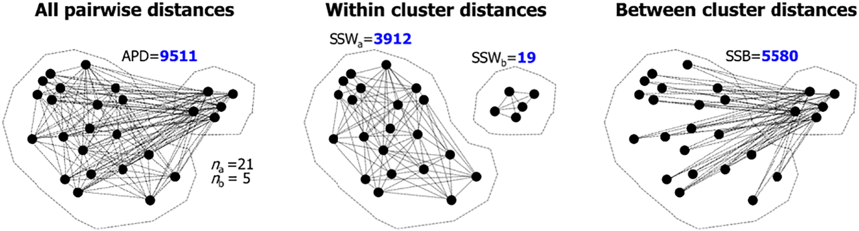
Figure 1: Example of APD (left), SSW (middle), and SSB (right). There are O(n2) links, but not all of them are drawn. The links have the following relationship: {APD} = {SSW}
2.3 Number of SSB Calculations
Motivated by the observations, we reformulate the k-means algorithm using between-cluster distances (SSB). However, this can be time-consuming because there are O(n2) pairwise distances to be calculated at every iteration, which is too slow. An alternative solution is to store the O(n2) size distance matrix, but this would reduce the practicality of the method due to quadratic memory consumption. Neither option looks very promising for scalability.
Fortunately, most SSB distances are between points located far away from each other, so they will almost never be assigned to the same cluster. In other words, they have no contribution to clustering. The distances that matter are points near each other so that they can sometimes belong to the same cluster depending on the operation of the algorithm. They contribute to the objective function most.
One possibility to make the method faster is to limit the distance calculations only between points in neighboring clusters. However, if the number of clusters is small (c << n), almost all clusters are neighbors. This can also happen when the dimension increases high because the distances tend to become equidistant when using Euclidean (L2) distance [32]. Minkowski distances (Lp) with other values of p have also been considered and L-norms with fractional values (0 < p < 1) have been shown to work better for high-dimensional data [33].
To demonstrate the problem, assume that the points are equally divided so that all clusters have size n/c points. In this case, there are (n/c)2 distances between every pair of clusters. If we compute distances only between the nearest cluster, there would still be c·(n/c)2 = n2/c distance calculations. If c =
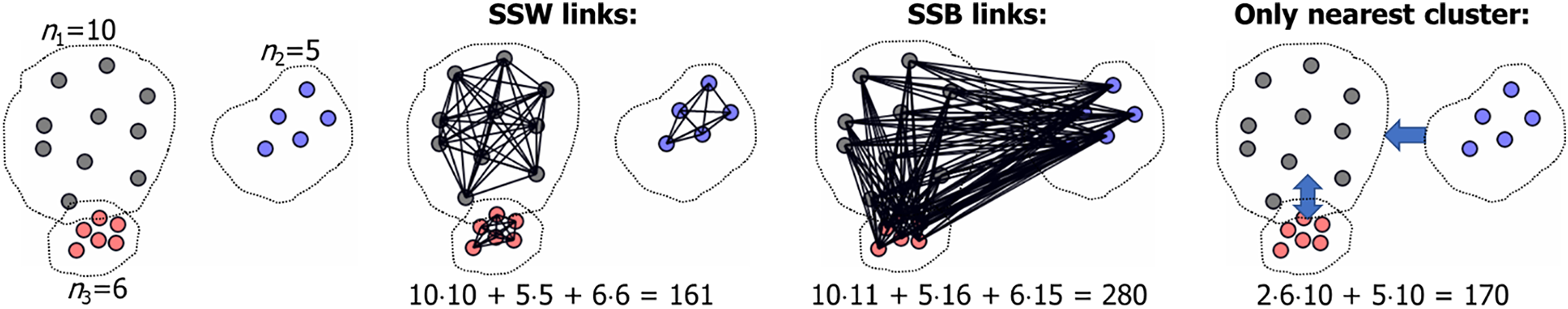
Figure 2: Total number of SSB calculations (280) and the number of calculations if only considering the nearest cluster (170)
When minimizing sum-of-squared Euclidean distances, the calculations can be done more efficiently. From (12), we know that the sum of squared distances (SSE), multiplied by n, equals all pairwise distances within the clusters (SSW):
This is already utilized in k-means by using the centroids to calculate the within-cluster distances (SSW). However, the result also generalizes between-cluster distances as shown in [27,34].
In other words, both SSW and SSB can be done in O(n) time via SSE. In the following, we do not utilize this property as we are interested in overlap. This requires point-level information that would be lost if we used centroids to represent the clusters. However, this property can be beneficial for others, and thus, it is presented here.
Among all the point pairs, the most meaningful ones are those that are near to each other but in different clusters. In other words, border pixels. In the proposed method, we, therefore, calculate only one distance per point to its nearest neighbor in another cluster. This distance is put into the context of its relative location in its own cluster.
We formulate a so-called overlap value for each data point based on the overlap measure proposed in [35]. The overlap score for a point xi is calculated as follows:
where
The lower the overlap value, the better the cluster assignment of the point. The new objective function then minimizes the sum of all overlap values in the data:
The overlap value includes two terms. The first term (numerator) represents a sample of the SSW function, and the second term (divider) is a sample of the SSB function. The overlap is, therefore, a strongly sampled version of the Calinski and Harabasz measure [25] and closely related to other sum-of-squared based indexes [27]. The difference is that the overlap measure is not normalized by the cluster size.
Example calculations are shown in Fig. 3, where the large cluster (gray points) has points near the small dense cluster (red points). While all border points have high distances to the centroids, only those near the red cluster have a high overlap value.
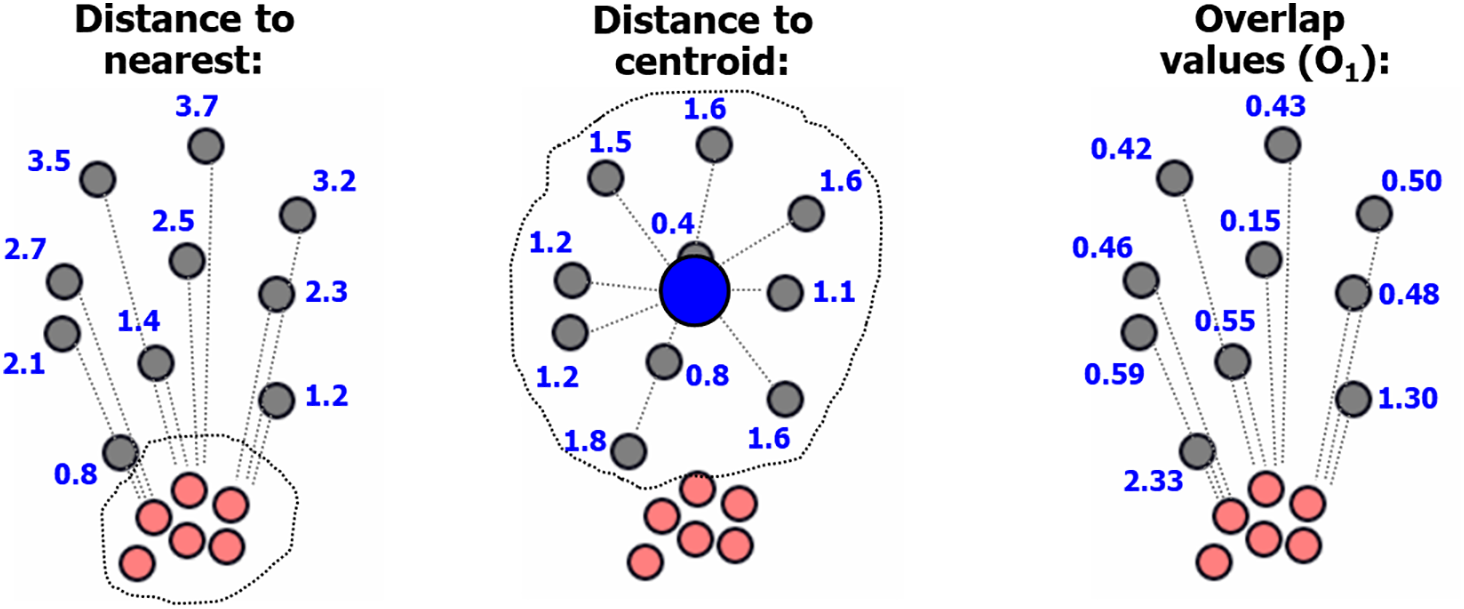
Figure 3: The proposed objective function calculates the distance from a point only to its nearest neighbor in another cluster and to its own centroid
K-means has two steps that should be updated according to the new objective function. Theoretically, the nearest cluster should be calculated by minimizing (16). However, we face computational problems. Finding the nearest neighbor point takes O(n) time for one point, and we have n points to process. The time complexity of the partition would, therefore, grow to O(n2). To avoid this, we keep the original k-means assignment and find the nearest centroid.
The second step is to calculate the centroid for the clusters. We calculate the weighted average so that every point is inversely weighted by its overlap value. In this way, the border points with high overlap values will have less impact on the centroid location, which will move closer to the non-border points. The exact update rule is as follows:
where

Despite the alternative formulation, Overlap k-means is merely another variant of k-means that optimizes essentially the same variables: minimizing SSW and maximizing SSB. The overlap score itself is localized regarding the SSB calculations by considering only the nearest neighbor in another cluster. The motivation was merely to reduce the calculations.
Next, we extend the localization to the SSW part by removing the dependency on the centroid. We want the overlap to be based only on local properties. To achieve this, we calculate a local neighborhood of a point defined by its k-nearest neighbors (KNN). Localized overlap value is then defined as:
where
where
The divider is the same in both
It is both an advantage and a disadvantage. The idea is that the higher the mean-shift distance, the more points differ from their neighborhoods. In specific, border points have high mean-shift values. This idea was originally developed for outlier detection in [36]. An example is shown in Fig. 4. Pseudo code of the local variant is given in Algorithm 2.
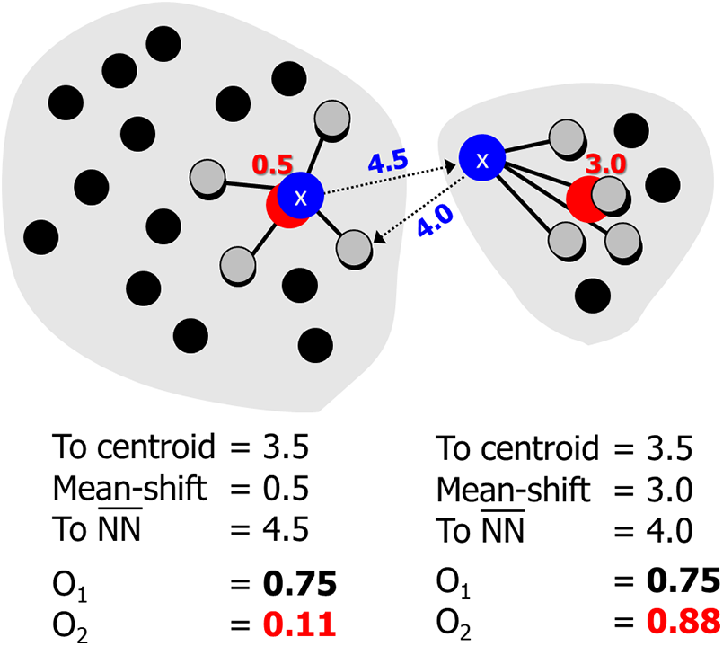
Figure 4: Two points (blue) having the same distance to their cluster centroid (3.5), almost the same distance to the nearest point in another cluster (4.5 and 4.0), but with very different mean shift values (0.5 and 3.0)

The datasets used in the experiments are listed in Table 1 and demonstrated in Fig. 5. We selected datasets from the clustering basic benchmark [35] and from [37]. The datasets have varying cluster overlaps, shapes, and densities.
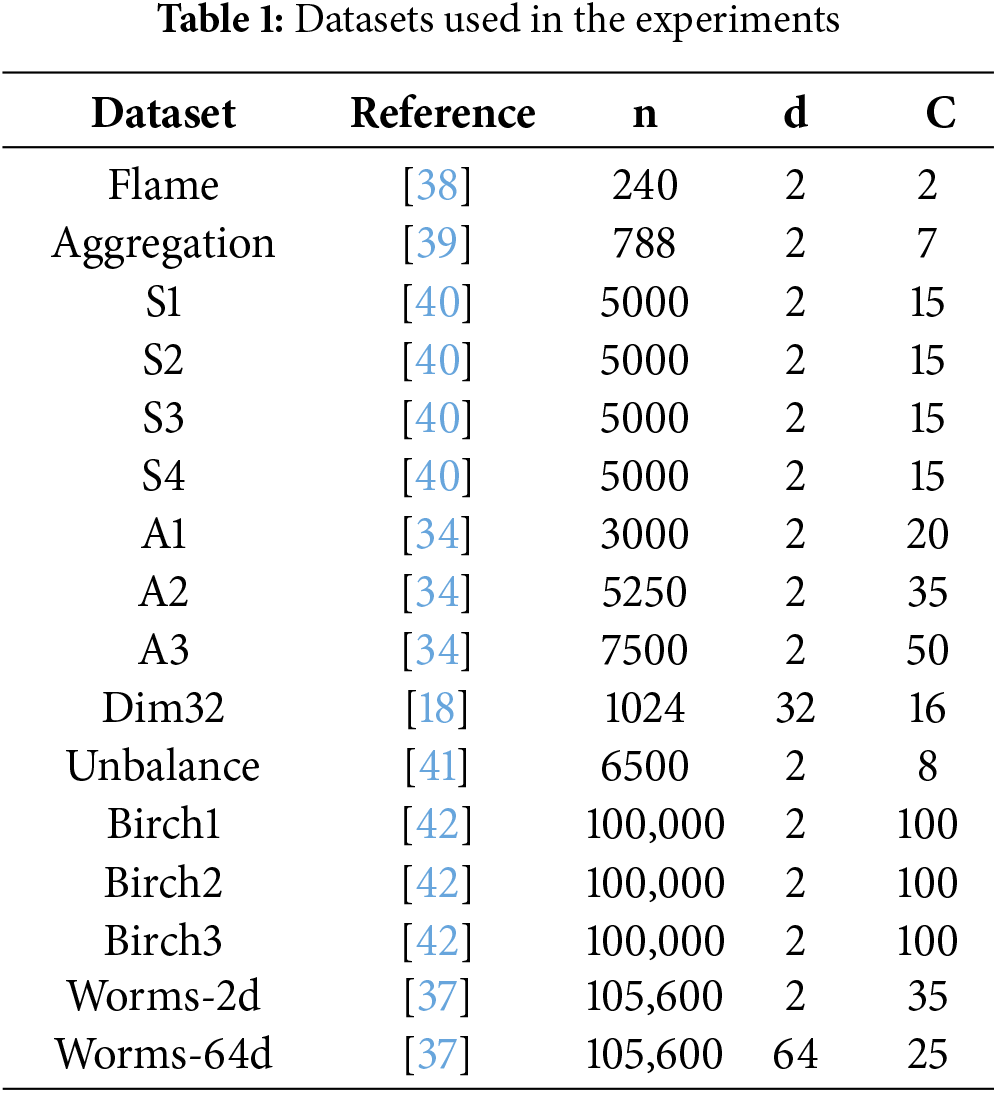
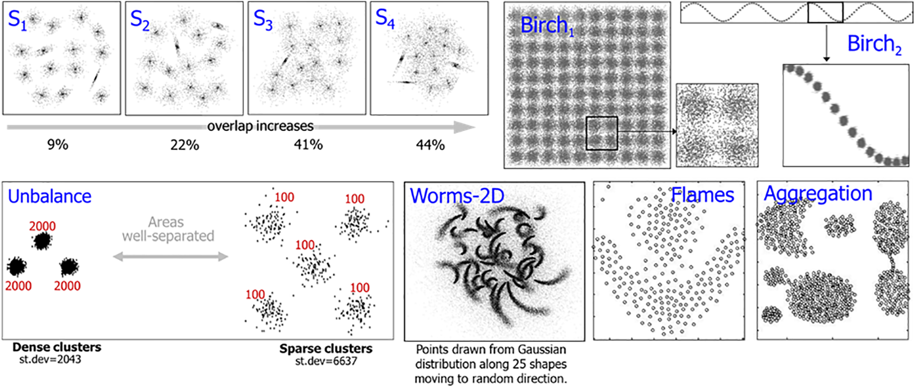
Figure 5: Visualization of the selected datasets. Some datasets are seemingly simple with regular structure (Birch1–3), whereas others have challenges like varying cluster overlap (S1–S4), density (Unbalance), or shapes (Worms-2D, Worms-64D)
We cluster the datasets with the following algorithms:
• K-means (KM)
• K-means++ (KM++)
• Random swap (RS)
• Density peaks (DensP)
• DBSCAN
• Spectral clustering (Spectral)
• Overlap k-means (OK)
• Localized variant (OK-local)
K-means is the main point of comparison to see whether Overlap k-means provides similar clustering results to the standard k-means with the same seeding method. K-means itself can be improved by simple tricks like repeats and better seeding [43]. We, therefore, also tested the most popular seeding called K-means++ [44], which is based on a randomized further point heuristic.
We also include random swap [5], which is almost as simple as k-means and provides a state-of-the-art reference to how good clustering accuracy one can expect by minimizing SSE. It is one of the few clustering algorithms that find the correct cluster allocation for all the benchmark data. Other algorithms included are density peaks [45], DBSCAN [46,47], and spectral clustering [48].
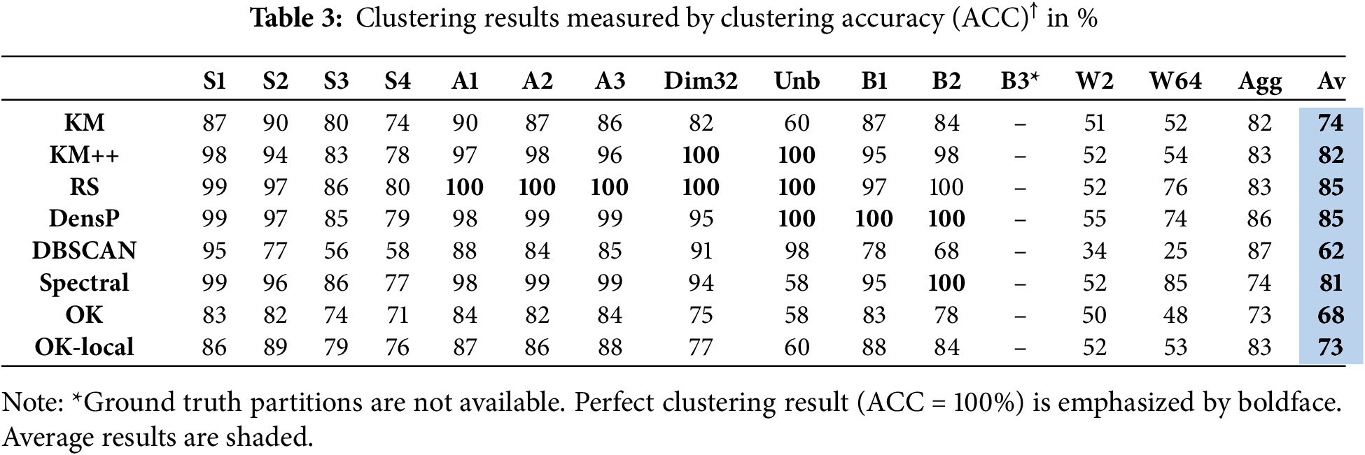
We run all algorithms 100 times and report the average results, with the exceptions of Birch and Worms datasets, which are repeated only 10 times due to their higher processing times. Clustering results are measured by clustering accuracy (ACC) [49] and centroid index (CI) [50].
We have two main hypotheses to test: (1) Does OK provide similar results to k-means, and (2) can OK-local find clusters having non-uniform shapes and density?
The main results are summarized in Tables 2 and 3. Good algorithms like Random swap and Density peaks can find correct clustering (CI = 0) for most datasets. They only fail with the non-spherical datasets Birch3, Worms, and Aggregation, which cannot be clustered correctly by the SSE objective function. K-means++ manages to solve Dim32 and Unabalance, whereas K-means does not solve any of the datasets (average CI = 5.8).
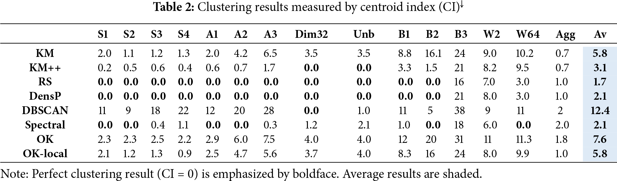
Beyond the clustering accuracy, the interest here is more on the comparison between k-means (KM) and its overlap variant (OK). The results of these two are indeed similar, but there is a noticeable difference favoring k-means. The localized variant provides results closer to k-means. The corresponding average CI values are 5.8 (K-means), 7.6 (OK), and 5.8 (Local-OK).
Our first hypothesis was that Overlap k-means would provide similar results to k-means, but the results do not support it. We analyze the reasons in Fig. 6 with the S1 dataset, which is easy for good algorithms but troublesome for k-means due to small cluster overlap [35]. The results show that k-means can move all centroids to their correct location except two. Overlap k-means, however, performs even worse with four clusters unsolved.

Figure 6: K-means and Overlap k-means result with S1 for the same initial solution (left). Overlap k-means positions the centroids better within the clusters but has problems locating them correctly globally. The CI-values of the solutions are CI = 2 (k-means) and CI = 4 (Overlap k-means) accordingly
The reason is studied in Fig. 7, where the pulling effect of the faraway points attracts a centroid in just three iterations with k-means. However, the same does not happen with Overlap k-means. The reason is due to the low weight of the faraway points in the centroid calculation. This leads to nicely balanced locations of the centroids within the same cluster but leaving the one above empty.
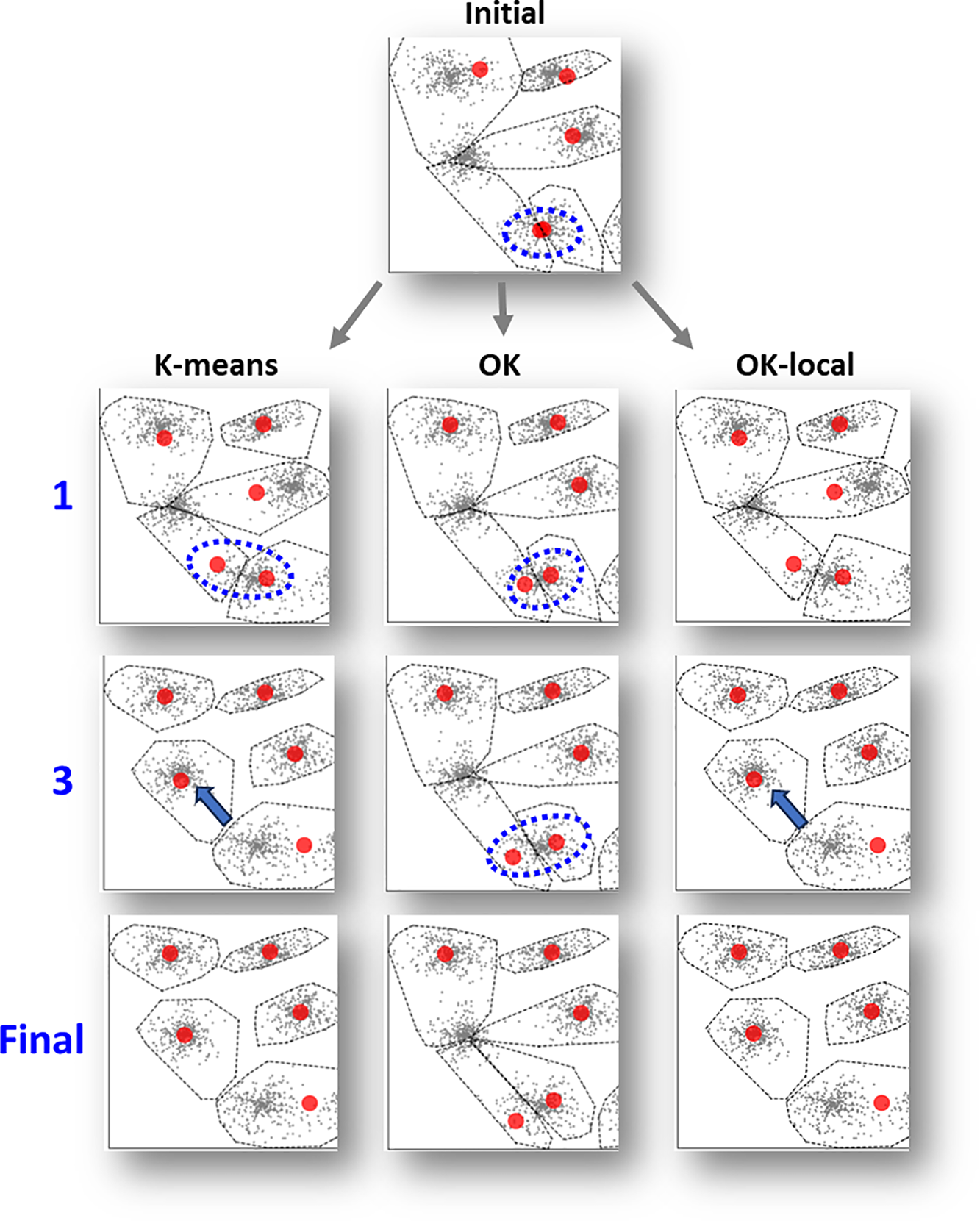
Figure 7: Snapshots of the bottom left corner of S1 after the 1st iteration, 3rd iteration, and the final solution. The pulling effect of the faraway points in k-means manages to move one of the centroids to the cluster missing a centroid. Overlap k-means gives less weight to the border points, which stabilizes the centroids close to their original location and makes the algorithm less dynamic
We conclude that it is possible to design k-means via the between-cluster distances, but the chosen design using the overlap is not good. It makes the algorithm practical by avoiding the overwhelming computations of the between-cluster distances, but it significantly reduces the pulling effect of the remote points, which is vital for k-means. In other words, the algorithm becomes too rigid and tends to get stuck in a local minimum. An effective algorithm should do the opposite: enhance the vital faraway boundary points instead of restricting their use.
The second hypothesis was that the localized variant could also work for non-spherical datasets. This does not happen either. The results of OK-local are closer to k-means than those of OK, but they do not perform any better with the non-spherical datasets (Birch3, Worms, and Aggregation). We cannot conclude whether the idea is not good enough or the potential is not fulfilled by the inferior local optimization.
We did not carry out further tests other than this proof-of-concept. The main contribution is theoretical, showing the connection between the within-cluster and between cluster distances. If one wants to achieve a better algorithm based on the overlap concept, we outline two potential ways to do it here.
1. Design a stochastic variant starting with the opposite: give high weight for the high overlap points. This would further enhance the dynamics of k-means, hopefully pushing the centroids even further than the standard SSE function would do. Then, decrease the weights and gradually converge to the Overlap k-means variant, which would focus on the central points.
2. Replace k-means with a better local optimizer: random swap. This would completely avoid the problem of local minima. If there are any benefits of the OK or OK-local, their random swap counterparts have a higher potential to exploit them.
We have the following conclusions:
First, within-cluster (SSW) and between-cluster distances (SSB) measure essentially the same quantity and do not offer any complementary information. K-means uses the sum-of-squared (SSE) objective function, which is essentially a scaled version of SSW. We have shown that the same objective can be constructed using between-cluster distances.
Second, if we calculate the centroids for the data, both approaches can be calculated in O(n) time [27,34]. Otherwise, we need to calculate all pairwise distances. Within-cluster distances (SSW) take k·(n/k)2 = O(n2/k) time in case of balanced cluster sizes. Between-cluster distances, on the other hand, require the calculation of all pairwise distances in the entire data, which leads to O(n2) time complexity.
Third, Calinski–Harabasz, silhouette score, WB-index, and DBI and most other internal indexes assume that both the within-cluster and between-cluster variances are needed. This paper demonstrates that this is not the case. The consequence is that all these indexes are heuristics based on wrong assumption, which implies that a better approach should be designed based on a different principle.
Fourth, we presented a new algorithm called overlap k-means (OK), which utilizes between-cluster distances. Instead of minimizing all distances, it focuses on the distances near the cluster borders. However, this construction lost the dynamics of the k-means algorithm, leading to a more rigid algorithm behavior. The results of the localized variant were more consistent with that of k-means.
Fifth, the overlap idea has further potential. We outlined two possibilities. The first one would be a stochastic variant, which would emphasize the border points more in the beginning and gradually reduce their effect, leading to the Overlap k-means. The second possibility would be simply to replace the inferior k-means with a more robust random swap algorithm. These two are points for future studies.
Acknowledgement: We thank Fei Wang and Le Li for their help.
Funding Statement: The authors received no specific funding for this study.
Author Contributions: Study conception and design: Pasi Fränti; theoretical part: Pasi Fränti and Qinpei Zhao; algorithm design and experiments: Claude Cariou; analysis and interpretation of results: Pasi Fränti and Claude Cariou; draft manuscript preparation: Pasi Fränti and Claude Cariou. All authors reviewed the results and approved the final version of the manuscript.
Availability of Data and Materials: The source code and the datasets generated during and/or analyzed during the current study are available in the https://cs.uef.fi/ml/software/, https://cs.uef.fi/sipu/datasets/ (accessed on 05 September 2025).
Ethics Approval: Not applicable.
Conflicts of Interest: The authors declare no conflicts of interest to report regarding the present study.
Appendix A: Pseudo Code of the Overlap k-Means
X = dataset
K = Size of KNN
NN = Nearest neighbors
NC = number of clusters
PerformOK(X, NC, K)
{
/* initial solution */
NN: = FindKNN(X,K);
C: = SelectRandomRepresentatives(X,NC);
P: = OptimalPartition(C,X);
P_old: = zeros(size(P));
O: = Overlap-v1(P,X,NN,C);
gamma = Mean(O);
WHILE P <> P_old
{
P_old = P;
(P,C,O): = OK-means(P,C,X,O,NN,gamma);
}
RETURN (P,C,O);
}
OK-means(P,C,X,O,NN,gamma)
{
/* performs one K-means iteration with KNN-overlap weighting */
C: = OptimalRepresentatives_w_Overlap(P,X,O,gamma);
P: = OptimalPartition(C,X);
O: = Overlap-v1(P,X,NN,C);
RETURN (P,C,O);
}
OptimalPartition(C,X)
{
FOR i: = 1 TO N DO
{
P[i]: = FindNearestRepresentative(C,X[i]);
}
RETURN P;
}
FindNearestRepresentative(C,x)
{
j: = 1;
FOR i: = 2 TO k DO
{
IF Dist(x,C[i]) < Dist(x,C[j]) THEN
{
j: = i;
}
}
RETURN j;
}
Overlap-v1(P,X,NN,C)
{
FOR i: = 1 TO N DO
{
B: = NN[i];
Q: = Points in X with label P[i];
T: = B ∩ (X \ Q) /*The nearest neighbors having a different label
D2: = SmallestDistance(T,X[i]); /*Smallest distance between X[i] and T*/
D1: = Dist(X[i],C[P[i]]); /*Dist. between X[i] and its centroid*/
O[i]: = D1/D2; /*Overlap cost*/
}
RETURN O;
}
OptimalRepresentatives_w_Overlap(P,X,O,gamma)
{
/* initialize Sum[1..k] and Count[1..k] by zero values! */
/* sum vector and count for each partition */
FOR i: = 1 TO N DO
{
j: = P[i];
Sum[j]: = Sum[j] + X[i]*exp(-(O[i]/gamma)**2);
Count[j]: = Count[j] + exp(-(O[i]/gamma)**2);
}
/* optimal representatives are average vectors */
FOR i: = 1 TO k DO
{
IF Count[i] <> 0 THEN
{
C[i]: = Sum[i]/Count[i];
}
}
RETURN C;
}
SmallestDistance(Data,Query)
{
Dmin: = some large positive value;
FOR i: = 1 TO N DO
{
D: = Dist(Data[i],Query);
IF D < Dmin THEN
{
Dmin: = D;
}
}
RETURN Dmin;
}
AvgDistance(D)
{
Sum = 0;
FOR i: = 1 TO K DO
{
Sum = Sum + D[i];
}
Davg: = Sum/K;
RETURN Davg;
}
References
1. Forgy E. Cluster analysis of multivariate data: efficiency vs. interpretability of classification. Biometrics. 1965;21:768–80. [Google Scholar]
2. MacQueen J. Some methods for classification and analysis of multivariate observations. In: Berkeley Symposium on Mathematical Statistics and Probability; 1965 Jun 21–Jul 18; Berkeley, CA, USA. p. 281–97. [Google Scholar]
3. Lloyd S. Least squares quantization in PCM. IEEE Trans Inf Theory. 1982;28(2):129–37. doi:10.1109/TIT.1982.1056489. [Google Scholar] [CrossRef]
4. Fränti P. Genetic algorithms for large-scale clustering problems. Comput J. 1997;40(9):547–54. doi:10.1093/comjnl/40.9.547. [Google Scholar] [CrossRef]
5. Fränti P. Efficiency of random swap clustering. J Big Data. 2018;5(1):13. doi:10.1186/s40537-018-0122-y. [Google Scholar] [CrossRef]
6. Malinen MI, Mariescu-Istodor R, Fränti P. K-means: clustering by gradual data transformation. Pattern Recognit. 2014;47(10):3376–86. doi:10.1016/j.patcog.2014.03.034. [Google Scholar] [CrossRef]
7. Fritzke B. Breathing k-means. arXiv:2006.15666. 2020. [Google Scholar]
8. Lee J, Perkins D. A simulated annealing algorithm with a dual perturbation method for clustering. Pattern Recognit. 2021;112(4):107713. doi:10.1016/j.patcog.2020.107713. [Google Scholar] [CrossRef]
9. Baldassi C. Recombinator-k-means: an evolutionary algorithm that exploits k-means for recombination. IEEE Trans Evol Comput. 2022;26(5):991–1003. doi:10.1109/TEVC.2022.3144134. [Google Scholar] [CrossRef]
10. Fränti P, Mariescu-Istodor R. Averaging GPS segments competition 2019. Pattern Recognit. 2021;112(2):107730. doi:10.1016/j.patcog.2020.107730. [Google Scholar] [CrossRef]
11. Malinen MI, Fränti P. Clustering by analytic functions. Inf Sci. 2012;217:31–8. doi:10.1016/j.ins.2012.06.018. [Google Scholar] [CrossRef]
12. Nie F, Xue J, Wu D, Wang R, Li H, Li X. Coordinate descent method for kk-means. IEEE Trans Pattern Anal Mach Intell. 2022;44(5):2371–85. doi:10.1109/TPAMI.2021.3085739. [Google Scholar] [PubMed] [CrossRef]
13. Qu F, Shi Y, Yang Y, Liu Y, Hu Y. Coordinate descent K-means algorithm based on split-merge. Comput Mater Contin. 2024;81(3):4875–93. doi:10.32604/cmc.2024.060090. [Google Scholar] [CrossRef]
14. Ward JHJr. Hierarchical grouping to optimize an objective function. J Am Stat Assoc. 1963;58(301):236–44. doi:10.1080/01621459.1963.10500845. [Google Scholar] [CrossRef]
15. Equitz WH. A new vector quantization clustering algorithm. IEEE Trans Acoust Speech Signal Process. 1989;37(10):1568–75. doi:10.1109/29.35395. [Google Scholar] [CrossRef]
16. Shanbehzadeh J, Ogunbona PO. On the computational complexity of the LBG and PNN algorithms. IEEE Trans Image Process. 1997;6(4):614–6. doi:10.1109/83.563327. [Google Scholar] [PubMed] [CrossRef]
17. Fränti P, Kaukoranta T, Shen DF, Chang KS. Fast and memory efficient implementation of the exact PNN. IEEE Trans Image Process. 2000;9(5):773–7. doi:10.1109/83.841516. [Google Scholar] [PubMed] [CrossRef]
18. Fränti P, Virmajoki O, Hautamäki V. Fast agglomerative clustering using a k-nearest neighbor graph. IEEE Trans Pattern Anal Mach Intell. 2006;28(11):1875–81. doi:10.1109/TPAMI.2006.227. [Google Scholar] [PubMed] [CrossRef]
19. Shi J, Malik J. Normalized cuts and image segmentation. IEEE Trans Pattern Anal Mach Intell. 2000;22(8):888–905. doi:10.1109/34.868688. [Google Scholar] [CrossRef]
20. Hagen L, Kahng AB. New spectral methods for ratio cut partitioning and clustering. IEEE Trans Comput Aided Des Integr Circuits Syst. 1992;11(9):1074–85. doi:10.1109/43.159993. [Google Scholar] [CrossRef]
21. Leskovec J, Lang KJ, Mahoney M. Empirical comparison of algorithms for network community detection. In: Proceedings of the 19th International Conference on World Wide Web; 2010 Apr 26–30. Raleigh, NC, USA. p. 631–40. doi:10.1145/1772690.1772755. [Google Scholar] [CrossRef]
22. Newman MEJ, Girvan M. Finding and evaluating community structure in networks. Phys Rev E. 2004;69(2):026113. doi:10.1103/physreve.69.026113. [Google Scholar] [PubMed] [CrossRef]
23. Sieranoja S, Fränti P. Adapting k-means for graph clustering. Knowl Inf Syst. 2022;64(1):115–42. doi:10.1007/s10115-021-01623-y. [Google Scholar] [CrossRef]
24. Cohen-Addad V, Kanade V, Mallmann-Trenn F, Mathieu C. Hierarchical clustering: objective functions and algorithms. J ACM. 2019;66(4):26. doi:10.1137/1.9781611975031.26. [Google Scholar] [CrossRef]
25. Calinski T, Harabasz J. A dendrite method for cluster analysis. Commun Stat Simul Comput. 1974;3(1):791519860. doi:10.1080/03610917408548446. [Google Scholar] [CrossRef]
26. Rousseeuw PJ. Silhouettes: a graphical aid to the interpretation and validation of cluster analysis. J Comput Appl Math. 1987;20:53–65. doi:10.1016/0377-0427(87)90125-7. [Google Scholar] [CrossRef]
27. Zhao Q, Fränti P. WB-index: a sum-of-squares based index for cluster validity. Data Knowl Eng. 2014;92:77–89. doi:10.1016/j.datak.2014.07.008. [Google Scholar] [CrossRef]
28. Hämäläinen J, Jauhiainen S, Kärkkäinen T. Comparison of internal clustering validation indices for prototype-based clustering. Algorithms. 2017;10(3):105. doi:10.3390/a10030105. [Google Scholar] [CrossRef]
29. Malinen MI, Fränti P. All-pairwise squared distances lead to more balanced clustering. Appl Comput Intell. 2023;3(1):93–115. doi:10.3934/aci.2023006. [Google Scholar] [CrossRef]
30. Bubeck S, von Luxburg U. Nearest neighbor clustering: a baseline method for consistent clustering with arbitrary objective functions. J Mach Learn Res. 2009;10:657–98. [Google Scholar]
31. Aloise D, Deshpande A, Hansen P, Popat P. NP-hardness of Euclidean sum-of-squares clustering. Mach Learn. 2009;75(2):245–8. doi:10.1007/s10994-009-5103-0. [Google Scholar] [CrossRef]
32. Beyer K, Goldstein J, Ramakrishnan R, Shaft U. When is “nearest neighbor” meaningful? In: International Conference on Database Theory; 1999 Jan 10–12; Jerusalem, Israel. Berlin/Heidelberg, Germany: Springer; 1999. p. 217–35. doi:10.1007/3-540-49257-7_15. [Google Scholar] [CrossRef]
33. Aggarwal CC, Hinneburg A, Keim DA. On the surprising behavior of distance metrics in high dimensional space. In: International Conference on Database Theory (ICDT’01); 2001 Jan 4–6; London, UK. Berlin/Heidelberg, Germany: Springer-Verlag; 2001. p. 420–34. doi:10.1007/3-540-44503-x_27. [Google Scholar] [CrossRef]
34. Kärkkäinen I, Fränti P. Dynamic local search algorithm for the clustering problem. Joensuu, Finland: University of Joensuu; 2002. Report No.: A-2002-6. [Google Scholar]
35. Fränti P, Sieranoja S. K-means properties on six clustering benchmark datasets. Appl Intell. 2018;48(12):4743–59. doi:10.1007/s10489-018-1238-7. [Google Scholar] [CrossRef]
36. Yang J, Rahardja S, Fränti P. Mean-shift outlier detection and filtering. Pattern Recognit. 2021;115(406–21):107874. doi:10.1016/j.patcog.2021.107874. [Google Scholar] [CrossRef]
37. Sieranoja S, Fränti P. Fast and general density peaks clustering. Pattern Recognit Lett. 2019;128(3–5):551–8. doi:10.1016/j.patrec.2019.10.019. [Google Scholar] [CrossRef]
38. Fu L, Medico E. FLAME, a novel fuzzy clustering method for the analysis of DNA microarray data. BMC Bioinform. 2007;8(1):3. doi:10.1186/1471-2105-8-3. [Google Scholar] [PubMed] [CrossRef]
39. Gionis A, Mannila H, Tsaparas P. Clustering aggregation. ACM Trans Knowl Discov Data. 2007;1(1):4. doi:10.1145/1217299.1217303. [Google Scholar] [CrossRef]
40. Fränti P, Virmajoki O. Iterative shrinking method for clustering problems. Pattern Recognit. 2006;39(5):761–75. doi:10.1016/j.patcog.2005.09.012. [Google Scholar] [CrossRef]
41. Rezaei M, Fränti P. Set matching measures for external cluster validity. IEEE Trans Knowl Data Eng. 2016;28(8):2173–86. doi:10.1109/TKDE.2016.2551240. [Google Scholar] [CrossRef]
42. Zhang T, Ramakrishnan R, Livny M. BIRCH: a new data clustering algorithm and its applications. Data Min Knowl Discov. 1997;1(2):141–82. doi:10.1023/A:1009783824328. [Google Scholar] [CrossRef]
43. Fränti P, Sieranoja S. How much can k-means be improved by using better initialization and repeats? Pattern Recognit. 2019;93(2):95–112. doi:10.1016/j.patcog.2019.04.014. [Google Scholar] [CrossRef]
44. Arthur D, Vassilvitskii S. K-means++: the advantages of careful seeding. In: ACM-SIAM Symposium on Discrete Algorithms (SODA’07); 2007 Jan 7–9; New Orleans, LA, USA. [Google Scholar]
45. Rodriguez A, Laio A. Machine learning. Clustering by fast search and find of density peaks. Science. 2014;344(6191):1492–6. doi:10.1126/science.1242072. [Google Scholar] [PubMed] [CrossRef]
46. Ester M, Kriegel HP, Sander J, Xu X. A density-based algorithm for discovering clusters in large spatial databases with noise. KDD. 1996;96(34):226–31. [Google Scholar]
47. Schubert E, Sander J, Ester M, Kriegel HP, Xu X. DBSCAN revisited, revisited: why and how you should (still) use DBSCAN. ACM Trans Database Syst. 2017;42(3):1–21. doi:10.1145/3068335. [Google Scholar] [CrossRef]
48. von Luxburg U. A tutorial on spectral clustering. Stat Comput. 2007;17(4):395–416. doi:10.1007/s11222-007-9033-z. [Google Scholar] [CrossRef]
49. Fränti P, Sieranoja S. Clustering accuracy. Appl Comput Intell. 2024;4(1):24–44. doi:10.3934/aci.2024003. [Google Scholar] [CrossRef]
50. Fränti P, Rezaei M, Zhao Q. Centroid index: cluster level similarity measure. Pattern Recognit. 2014;47(9):3034–45. doi:10.1016/j.patcog.2014.03.017. [Google Scholar] [CrossRef]
Cite This Article
 Copyright © 2025 The Author(s). Published by Tech Science Press.
This work is licensed under a Creative Commons Attribution 4.0 International License , which permits unrestricted use, distribution, and reproduction in any medium, provided the original work is properly cited.
 Downloads
 Citation Tools