Solar Radiation Prediction Using Boosted Coyote Optimization Algorithm with Deep Learning for Energy Management

1  Introduction

As the population of the world increases, the demand for electrical energy also rises. At present, nearly 80% of the energy is generated from fossil fuels worldwide, as stated by the International Energy Agency (IEA) [1]. As usage of fossil fuel emits undesirable gases that adversely affect the climate alternate renewable energy resources need to be harnessed [2]. The technology of Solar photovoltaic (PV) is gaining more attention as an alternative to conventional energy. The benefits of utilizing such technology are plentiful, and the relatively lower LOCE of solar power and their modularity has potential to be uses as a major source energy [3]. Predicting Global Horizontal Irradiance (GHI) is definite as the complete irradiance from the Sun assessed on a horizontal surface on the Earth and calculated in units of (W/m2), is a vital stage in most PV power forecast methods [4]. The dynamics of GHI are based on both stochastic and deterministic features, and the latter needs the acceptance of compound statistical and physical methods for effective prediction. So, the highly variable nature of solar energy over time, owing to its seasonality and the occurrence of clouds overhead, creates the PV technology extremely reliant on environmental states [5]. The intermittence of solar power production forces the grid operators to accept more compound management tactics to protect the equilibrium between supply and demand. Therefore, precise real-time and future solar energy predictions can be very beneficial to ensure the effective utilization of solar power [6].

Previous research studies on solar energy have projected a significant number of data-driven approaches for both long- and short-term predictions [7]. These methods fall into four main categories, which include physical models, statistical analysis, deep learning (DL), and machine learning (ML) techniques. In traditional prediction methods, the atmosphere’s physical conditions and dynamic gestures are characterized by utilizing a set of formulations. The performance of physical models heavily relies on the quality and quantity of climatological variables and solar cycle data [8]. Statistical techniques apply mathematical analysis to various input features for solar radiation forecasting. Commonly used methods include Auto-Regressive (AR) models, Exponential Smoothing, Auto-Regressive Integrated Moving Average (ARIMA), the Markov Chain method, and Gaussian Processes [9]. In the past few years, the use of artificial intelligence (AI)-based techniques has gained significant attention in the field of solar energy forecasting [10]. Preceding studies signify that AI-based methods are capable of delivering more precise predictions of solar radiation outcomes than other methods like unsupervised and supervised artificial neural networks (ANNs), support vector machine (SVM), DL models, etc.

This article presents a new Solar Radiation Prediction utilizing a Boosted Coyote Optimization Algorithm with Deep Learning (SRP-BCOADL) model for Energy Management. The SRP-BCOADL model begins by normalizing the input data using a min-max normalization approach to enhance robustness across different data scales. Additionally, the SRP-BCOADL technique employs DLSTM-AE network for accurate forecasting solar energy levels. The effectiveness of the DLSTM-AE model can be improved by the design of a hyperparameter optimizer using BCOA. The performance analysis of the SRP-BCOADL technique is tested using solar radiation data. The extensive experimental outcomes prove that the SRP-BCOADL method obtains more precision over other existing techniques across various measures.

2  Literature Survey

Waheed and Xu [11] demonstrated and incorporated a DL neural network method with analysis of time series and feature selection (FS). The deep feed-forward and deep neural networks (DNN) methods include stacking hidden layers (HL) of CNN like GRU and LSTM elements for controlling uncertainty. Additionally, random forest (RF) regression with Grid Search CV was employed to classify an optimum set of features. In [12], an image processing-based DL technique for short-term solar prediction was proposed. The shi Tomasi model is used to define the feature point on the imageries while the Lucas-Kanade optical flow technique was used to follow the defined feature point on the successive imageries. The average cloud velocity and direction were estimated using a linear regression model based on the tracked cloud movements. Lastly, short-term solar energies were assessed utilizing the LSTM-DL model. Quiñones et al. [13] use Encoding–Decoding Sequence-to-Sequence (Seq2Seq) methods with dual dissimilar RNN architecture, which are LSTM, and GRU methods. The techniques were trained utilizing climatological data attained from climate places. Additionally, an ensemble model was utilized to quantify the uncertainty in the forecasts, thereby increasing the confidence level for end-users in microgrid environments when making predictive decisions.

Sulaiman and Mustaffa [14] proposed a combination of recent meta-heuristic model such as the Evolutionary Mating Algorithm (EMA), to optimize the biases and weights of the DNN method. The research work uses a Feed Forward Neural Network (FFNN) to estimate AC power output using real solar power plant data, verified at 15-min intervals. Irshad et al. [15] presented an Arithmetic Optimizer with a Hybrid DL-based Solar Radiation Prediction (AOHDL-SRP) method. The developed AOHDL-SRP method tracks a 3-phase procedure such as prediction, hyperparameter optimizer, and pre-processing. Mainly, the AOHDL-SRP system contains the min-max normalization model to regularize the input data to an even format. Also, the offered AOHDL-SRP technique uses HDL utilizing CNN with an attention-oriented LSTM (ALSTM) method. Lastly, the AOA is used as the hyperparameter optimizer of the HDL method. The main objective of Ghimire et al. [16] is to project a progressive hybrid prediction technique that incorporates an FS mechanism utilizing a Slime-Mould Algorithm, followed by CNN, LSTM, and subsequently a CNN with Multilayer-Perceptron as the output layer. Comprehensive benchmarking of the obtained results against two DL models and three ML methods highlights the superior performance of the proposed prediction approach.

Ehteram et al. [17] developed an enhanced LSTM method to evaluate solar energy data and create a collective procedure among gates. The study enhances the efficacy of LSTM gates. Climate data are employed. The Boruta-RF (BRF) FS algorithm was employed to define the finest input state. The RLSTM technique was equated with the LSTM method, RNN, radial basis function NN (RBFNN), and the Bi-LSTM method. Ghimire et al. [18] proposed an advanced hybrid model that incorporates CNN with multi-layer Perceptron (MLP) to produce global solar radiation (GSR) predictions. The CMLP method initially removes optimum topological and basic features fixed in prognostic variables over a CNN-based feature extractor phase tracked by an MLP-based analytical technique to produce GSR predictions. A hybrid-wrapper FS technique utilizing an RF-recursive feature elimination (RF-RFE) system is deployed to remove the terminated predictor feature.

Alkhatib et al. [19] investigate hourly GHI forecasting using both univariate and multivariate DL methods. This study specifically evaluates LSTM, CNN and a hybrid CNN/LSTM model. The finding that individual CNN and LSTM models generally outperform their hybrid counterpart offers a nuanced perspective on model complexity. This highlights the importance of empirical valuation and comparative analysis of modern selection instead of assuming that increasing complexity would lead to improved performance.

Rajendran and Gebremedhin [20] introduced the development and deployment of an ANN based forecasting model for solar power generation, specifically designed for integration with Energy PLAN simulation tools. It addresses common deep learning challenges such as overfitting through the implementation of techniques like dropout layers and emphasizing the importance of optimizing hyper parameters using tools like WANDB to ensure robust model performance on unseen data.

This paper focuses on the system level impact within microgrids rather than a detailed comparison of different deep learning models for forecasting accuracy.

Yadav et al. [21] compare various models like radial basis function neural network, LSTM, modular neural network and transformer models to predict daily global solar radiation, particularly in regions where direct measurements are imprecise or unavailable. These models are evaluated using different combinations of meteorological variables. The inclusion of the Transformer model suggests that the field of AI-based solar forecasting is rapidly adopting cutting edge advancements for broader area research.

The model they have proposed doesn’t have universal applicability.

Brahma and Wadhvani [22] concluded that integrating data from multiple sites significantly improves forecast performance compared to models trained solely on single location univariate data. It highlights the effectiveness of bidirectional LSTM and attention-based LSTM models for forecasting daily solar radiation. This approach helps address the challenges of data scarcity at individual sites.

This paper fails to compare the performance matrix across all models. The complexity of integrating and processing data is not discussed.

Mariappan et al. [23] proposed a hybrid deep learning model that integrates CNN and staked LSTM for the prediction of daily average solar irradiance, leveraging real time meteorically parameter and historical solar irradiance data. The authors infer that the model is highly effective at capturing long term dependencies in sequential data. Also, the systematic optimization of hyper parameters using a metaheuristic algorithm ensures that the designed architecture operates at its global or near global optimum thereby maximizing its predictive accuracy and robustness.

The requirement of higher computational demands because of the complexity of the model is not addressed.

Jang et al. [24] integrated classifier modules that identify site similarities to forecast solar power generation at unknown sites. By learning and identifying common patterns or clusters among diverse sites, the shared models can effectively generalize their learned knowledge from known sites to new, unseen locations. This adaptive mechanism reduces the need for extensive site-specific data for every new solar installation.

The internal working of the classifier module and the process by which it extracts site-specific features are not fully detailed in this paper.

3  Proposed Methodology

In this article, we have presented a new SRP-BCOADL model for energy management. The SRP-BCOADL model comprises of three main stages namely data normalization, DLSTM-AE-based solar radiation prediction, and BCOA-based parameter selection. Fig. 1 illustrates the entire procedure of the SRP-BCOADL model.

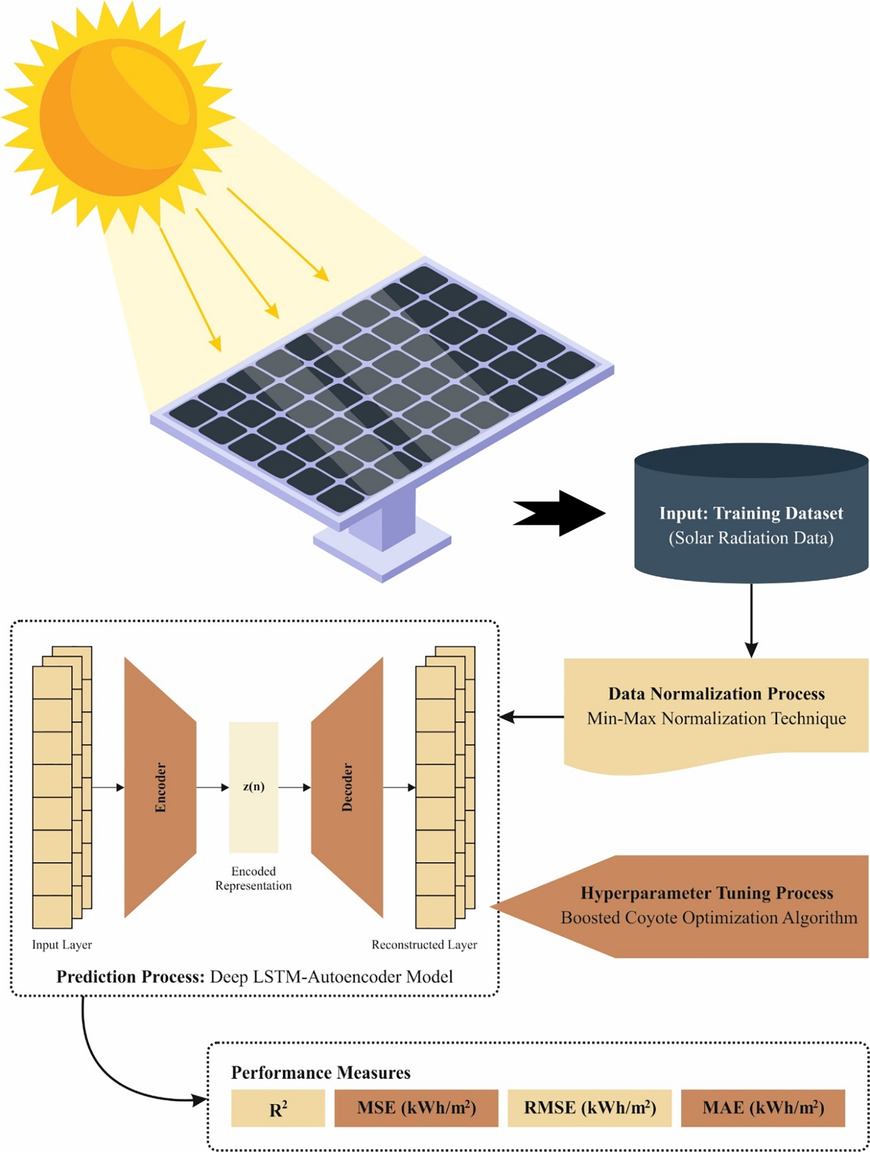
Figure 1: Overall process of SRP-BCOADL model

3.1 Data Normalization

Primarily, the SRP-BCOADL technique involves the normalization of the input data using a min-max normalization approach to improve the robust nature under different scales. In the structure of DL methods, the dataset often contains a wide range of data types, where features with larger numerical values can disproportionately influence the model, while the impact of features with smaller numerical values is diminished [25].

To address this problem, this research utilizes the min-max normalization model during the data pre-processing phase. This method effectively scales the data and reduces the disparity among feature values, thereby enhancing the model’s generalization capability to unseen data and helping to mitigate the risk of overfitting. The mathematical formulation for this technique is revealed in Eq. (1).

xnormal=x−xminxmax−xmin(1)

Here, xnormal denotes the value attained after normalization; x signifies the data to be standardized; xmin indicates the least value; and xmax refers to the maximum value.

3.2 Solar Radiation Prediction Process

Next, the SRP-BCOADL technique uses the DLSTM-AE network for predicting solar radiation levels. As mentioned before, the second element of a DLSTM network contains three LSTM layers [26]. The input pattern is a 3D tensor, representing the time sequence order. A sequence represents only one sample, a time-step represents one point of observation within the model, and a time-step is a single surveillance for each sequence. The architecture of the LSTM network used for the model generation is based on data collection. The volume of HL defines the output size. When determining the LSTM capacity, the number of units shall be considered; therefore, the more the units, greater are the learning capacity of LSTMs. The 1st, 2nd, and 3rd layers of HLs are defined as 200, 100, and 200 units, correspondingly. The output layer is a dense layer with three HLs that forecast all the values in the following 20 min depending on data from the latter 200 min. There is a choice in the LSTM layer known as “return-sequence”. Since the return sequence is fixed to False by default, only the last time step HL of the existing series is taken as an output. On the other hand, the output of LSTMs will consist of each hidden state from every time-step in the series by setting the return sequence to True. In the proposed LSTM model, the return sequence is fixed to true for the 1st and 2nd HLs which have 200 and 100 units, correspondingly. Furthermore, the return-sequence is set to False for the last HL, which contains 200 units. Lastly, if the return-state choice of the LSTM layer is fixed to True, ct is given back as an output together with ht. A batch size of 64 was used in this study. Before the weights are updated, the size of the batch is the volume of samples, which must be noted by the system. Moreover, dropout regularization avoids over-fitting during training. The dropout will fix the output of HLs randomly to 0 during training. The dropout rate is fixed at 0.1. The xt, ht, and ct are parameters representing the inputs of the LSTM unit, HL is the output of the LSTM block, and a vector of cell state, correspondingly. Moreover, the σ and ot are parameters representing the sigmoid function that determines which data should be disregarded from the output and input vectors.

Eqs. (2) to (9) represents how to define the forget gate ft, input gate it, and output gate ot. The data that is discarded from the cell state is defined by considering Wf and bf as weight and bias vectors of the forget gate, correspondingly:

ft=σ(Wf.[ht−1,xt]+bf)(2)

Eq. (3) is used for calculating what data to be stored in the cell state. Wi and bi are parameters that define the output weight matrix and bias of the input gate, correspondingly.

it=σ(Wi.[ht−1,xt]+bi)(3)

ot=σ(Wo.[ht−1,xt]+bo)(4)

Eq. (4) is used for managing data updating and exploiting data in the output gate. The Wo and bo are parameters representing the weight matrix and bias of the output gate, correspondingly.

The update of c (t − 1), the old cell state is defined into ct, the novel cell state:

ct=ft∗ct−1+it∗tanh(Wc.[ht−1,xt]+bc)(5)

In Eq. (5), Wc and bc denote the weight matrix and bias vectors of cell state, correspondingly. The hidden-sate vector is attained by the following equation

ht=ot∗tanh(ct)(6)

The ft, it, and ot are ANNs of a unique type known as FFNN that vary from other ANNs, which link among their nodes. Intrinsically, it varies from its descendant, RNN which uses a sigmoid function for regulating data flow. All the gates are used to receive 3 input vectors: the input vector of the existing time-step; the HL vector of the previous timestep; and the vector of cell state derived from the previous or current timestep.

The auto encoder (AE) reduction and DLSTM methods are combined to construct the predictive mechanism. The AE is used with three layers for automatically selecting features and learning encoded features. The AE is introduced for learning the behaviors over time series with dissimilar patterns. This enables the model to capture relationships within the series and generate useful features with a fixed dimensionality, resulting in reduced input feature complexity. The encoder captures the unusual behaviors of input that are fed into the prediction models.

3.3 Parameter Optimizer

Finally, the effectiveness of the DLSTM-AE model can be improved by the design of a hyperparameter optimizer using BCOA. Nature serves as a vital source of inspiration for humanity, offering solutions to complex and challenging problems across various scientific fields through its fascinating and intricate phenomena [27]. Numerous types of optimizers follow meta-heuristic models that mimic natural processes to solve optimization problems. Coyotes belong to the class of carnivorous mammals, with the majority of their population residing in Central and North America. Noteworthy, the coyote is known for its intelligence and exhibits complex behavior. The COA is inspired by the coyote’s adaptation to its surrounding environment and the collective intelligence exhibited within the pack. The COA adopts a strategic approach that aims to maintain a balance between exploration and exploitation.

The procedure starts with Np, which signifies the number of individuals, and Nc denotes the number of coyotes as candidate solutions. The cost function of the COA is determined based on the social behaviors of coyotes. Therefore, the coyote’s social behaviors are defined as:

SOCcg,c=z=[z1,z2,…,zD](7)

where n, g, and t demonstrate the number, group, and imitation time representation for the variable’s method, correspondingly.

Primarily, the coyotes’ numbers are elected arbitrarily and created as the individual outcomes from the searching region.

SOCcig,c=LBj+η×(Hrj−Lrj)(8)

In which, η∈[0,1] is a random amount and Lrj and Hrj demonstrate min and a max of the j-th parameter on the searching region.

The cost function of all the coyotes is evaluated by the following equation:

objcg,c=f(SOCcig,τ)(9)

The group position undergoes renewal through a random process. Moreover, individuals’ situations vary, and they change their situation by moving to other groups.

Gi=0.005×Nc2(10)

which is c≤√200, and the Gi’s amount is one or more. Based on the procedure’s boosted variation like social behaviors among coyotes, the count of groups’ associates can be constrained and could not be above 14 coyotes. The outcome is exemplified by the alpha formula mentioned below:

αg,t=soccg,tforminobjcg,t(11)

The following formula elucidates the typical social behavior changes among coyotes:

culjg,t={RNc+12,jg,t,Ncisoddnumber12(RNc2,jg,t+RNc2g,t+1,j)O.W.(12)

where RNcg,t defines the grouping of coyotes’ social condition for (g) as a group number at a time (t) for j.

The coyote’s life is a group of problems of environment and coyotes parent selection can be employed in the COA.

Blejg,t={socr1,jg,t,rj<grsorj=j1socr2,jg,t,rj≥grs+graorj=j2σj,O.W.(13)

where rj ∈ [0, 1] and r2 imply the random cost and coyote from g, randomly generated proposal variables are determined by j1 and j2, a range of proposal variable is signified by σj, and grs, gra defines the scatter and connection likelihoods that exemplify the diversity preservation mechanism of coyotes within the group. The grs and gra are represented by the next equation:

grs=1d(14)

gra=12(1−grs)(15)

In which, d signifies the dimensional of variables. Both elements calculating δ1 and δ2 describe the cultural substitute among the groups:

δ1=αg,t−soccr1g,t(16)

δ2=culg,t−soccr2g,t(17)

Whereas the culture differences among alpha (leader), and cr1 (elected coyote) are determined by δ1, and δ2 refers to the cultural differences among the cr2 (opted coyote) and set culture’s progress.

The following equation is employed for renewal of social behavior based on the effect of the group and leader:

nsoccg,t=soccg,t+r1×δ1+r2×δ2(18)

where r_1 and r_2 signify the interval of zero to one that is random selection. By assuming the novel formulas, the original cost is determined by the next formula:

nobjcg,t=f(nsoccg,t)(19)

soccg,t+1={nsoccg,t,nobjcg,t<objcg,tsoccg,t,O.W.(20)

The most essential characteristic of these methods is the capability to overcome the local optimum point.

Based on the explanations, it is understood that when individuals are randomly selected within each age group, it is likely to result in faster convergence, thereby improving the runtime performance.

Numerous different methods are projected to manage this issue. Lévy fight (LF) device is the most common method for raising bio-inspired effectiveness. The LF is offered by the following calculation that is planned based on the random pace efficiency to attain the local search condition:

Lf(w)≈w−1−τ(21)

w=H/|Z|1/τ(22)

σ2={sin⁡(πτ2)21+τ2×Γ(1+τ)τΓ(1+τ2)}2τ(23)

Whereas the Lf device is explained by τ = 1.5, the step-size and Gamma function are determined as w,Γ(⋅)Z∼N(0,σ∧2) and A∼N(0,σ∧2), correspondingly. This method of repeating formulization is based on Lf is determined by:

socc,newg,t+1t{soccg,t+1+Lf(σ)×f(soccg,t+1)rand>0.5soccg,t+1−Lf(σ)×f(soccg,t+1)rand≤0.5(24)

But the cost function for best and worst performances for group behavior is represented by f(soc_(c,worst)∧(g,t+1)) and f(soc_(c,best)∧(g,t+1)).

For evolving the method, the disorder device is presented as the next component. A widespread equation is demonstrated for the disorder device as follows:

CMi+1j=f(CMij),j=1,2,…,D(25)

D and f(CMij) demonstrate the dimensionality of the mapping and generator function.

During this work, a chaotic map has been employed for developing the COA for addressing this issue of rapid convergence. Specifically, the disorder device can be employed to discover a clarification for a local optimum problem that results in an inappropriate analysis with rapid convergence. To address this, pseudo-random standards can be employed. The disorder device can be utilized in 3 process variables (η,r_1,r_2).

ηk+1new=a(ηknew)2sin⁡(πηknew),(26)

r1newk+1=a(r1,newk)2sin⁡(πr1,newk),(27)

r2,k+1new=a(r2,knew)2sin⁡(πr2,knew),(28)

(η0new,r1,0new,r2,0new)∈[0,1],a∈(0,4](29)

where k refers to the repetition’s number. Fig. 2 represents the flowchart of BCOA.

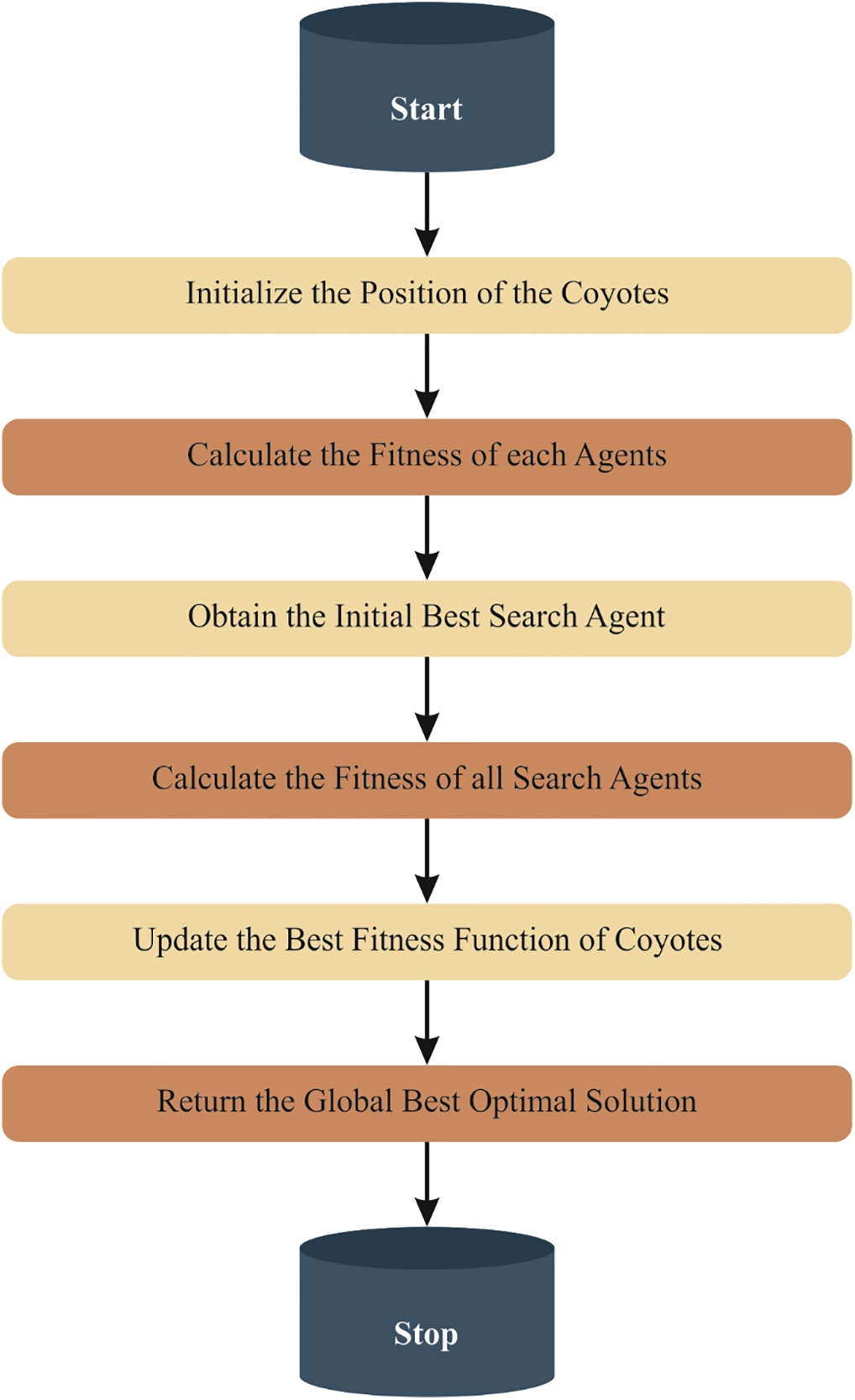
Figure 2: Flowchart of BCOA

Fitness choice is a major aspect controlling the solution of BCOA. The parameter selection method includes a solution-encoded model to evaluate candidate performance. In this context, the BCOA adopts an initial condition to define the fitness function.

4  Experimental Validation

This section inspects the performance analysis of the SRP-BCOADL technique. Table 1 and Fig. 3 deliver a complete set of solar radiation prediction outcomes of the SRP-BCOADL technique under 5 runs. The results indicate that the OMBGRU-SRP method has improved forecast outcomes. The figure denotes the actual vs. prediction of the SRP-BCOADL. The outcome shows that the SRP-BCOADL techniques have improved predicted results under every hour of operation. The variance between the predicted and actual solar radiation values is minimum.

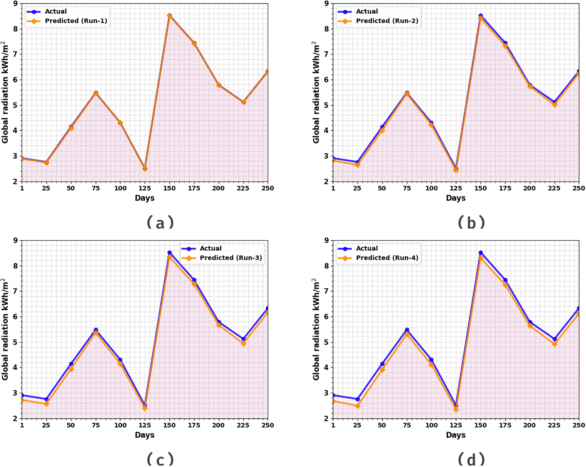
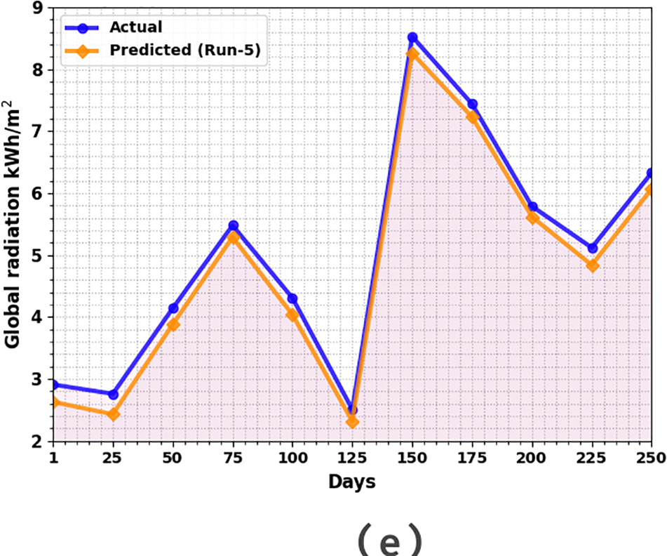
Figure 3: Global radiation of SRP-BCOADL technique (a–e) Runs 1–5

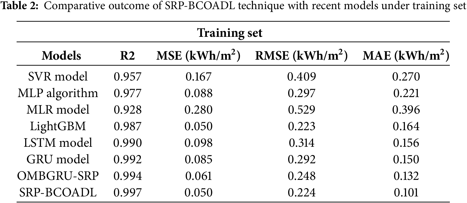
Table 2 represents the predictive results of the SRP-BCOADL technique and other existing models on the training set (TRS). The results imply that the SRP-BCOADL technique is sound [28,29].

In Fig. 4, a comparative R2 analysis of the SRP-BCOADL technique is reported on the TRS. The figure highlighted that the MLP and SVR models have exhibited lower R2 of 0.957 and 0.928, respectively. At the same time, the MLR, Light GBM, LSTM, GRU, and OMBGRU-SRP models obtained higher R2 of 0.928, 0.987, 0.990, 0.992, and 0.994, respectively. Nevertheless, the SRP-BCOADL technique gains maximum performance with an R2 of 0.997.

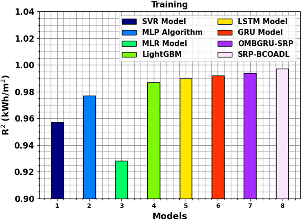
Figure 4: R2 outcome of SRP-BCOADL technique under training set

A comparison study of the SRP-BCOADL technique in terms of MSE is demonstrated in Fig. 5. The results point out that the SRP-BCOADL technique obtains better performance with the lowest values of MSE. It is noticed that the SRP-BCOADL technique gains improved results with the least MSE of 0.050 kWH/m2 while the SVR, MLP, MLR, LightGBM, GRU, and OMBGRU-SRP models portrayed lower MSE of 0.957, 0.977, 0.928, 0.987, 0.990, 0.992, and 0.994 kWH/m2, respectively.

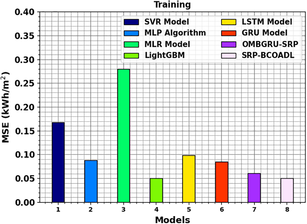
Figure 5: MSE outcome of SRP-BCOADL technique under training set

A comparison study of the SRP-BCOADL technique in terms of RMSE is established in Fig. 6. The outcomes pointed out that the SRP-BCOADL method shows better performance with minimum values of RMSE. It is observed that the SRP-BCOADL system attains enhanced results with minimum RMSE of 0.224 kWH/m2 while the SVR, MLP, MLR, Light GBM, GRU, and OMBGRU-SRP approaches have represented lower RMSE of 0.409, 0.297, 0.529, 0.223, 0.314, 0.292, and 0.248 kWH/m2, correspondingly.

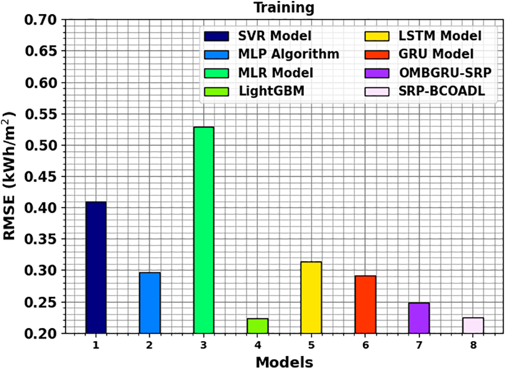
Figure 6: RMSE outcome of SRP-BCOADL technique under training set

A comparison study of the SRP-BCOADL method in terms of MAE is established in Fig. 7. The outcomes points that the SRP-BCOADL method gives better performance with the smallest values of MAE. It is perceived that the SRP-BCOADL model gains enhanced outcomes with minimum MAE of 0.101 kWH/m2 whereas the SVR, MLP, MLR, Light GBM, GRU, and OMBGRU-SRP approaches have portrayed lesser MAE of 0.270, 0.221, 0.396, 0.164, 0.156, 0.150, and 0.132 kWH/m2, correspondingly.

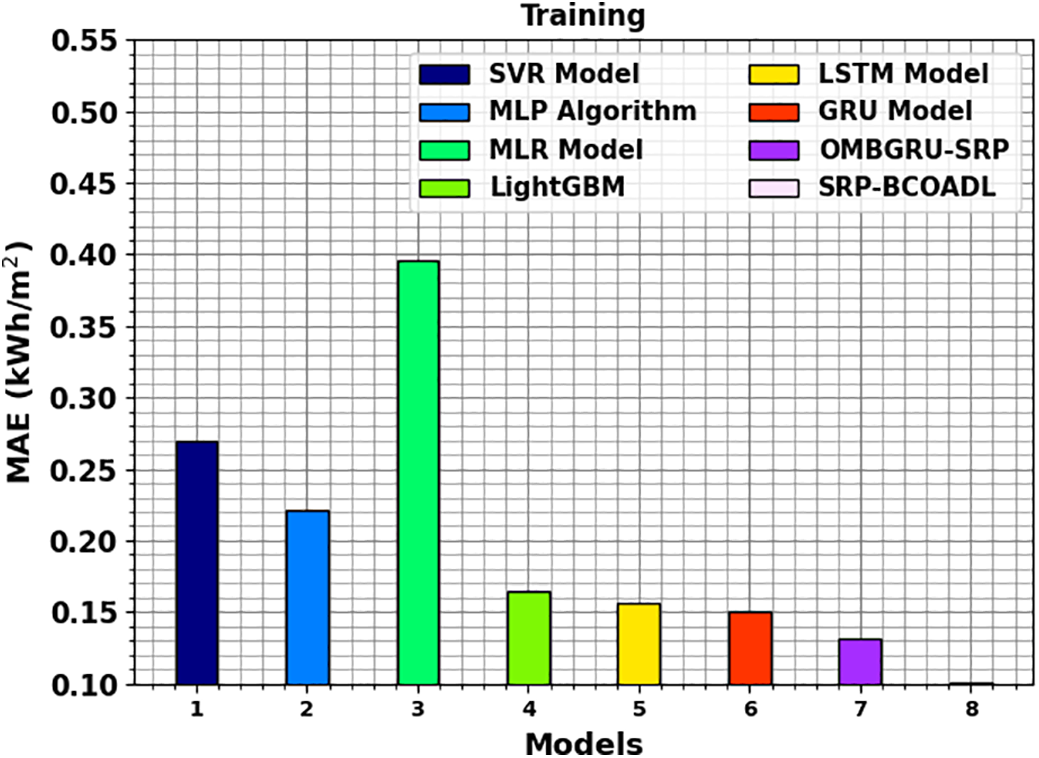
Figure 7: MAE outcome of SRP-BCOADL technique under training set

Table 3 signifies the predictive outcomes of the SRP-BCOADL system and another present method on the testing set (TSS). The outcomes suggest that the SRP-BCOADL model gains enhanced predictive outcomes. In Fig. 8, a comparative R2 analysis of the SRP-BCOADL system is stated on the TSS. The figure emphasized that the MLP and SVR techniques displayed less R2 of 0.929 and 0.937, respectively. Simultaneously, the MLR, Light GBM, LSTM, GRU, and OMBGRU-SRP approaches have gained greater R2 of 0.921, 0.938, 0.941, 0.943, and 0.945, respectively. Nevertheless, the SRP-BCOADL method gains the highest performance with an R2 of 0.959.

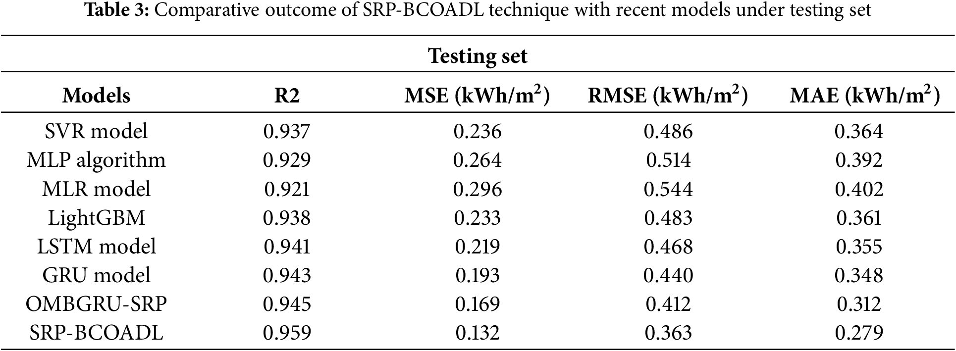
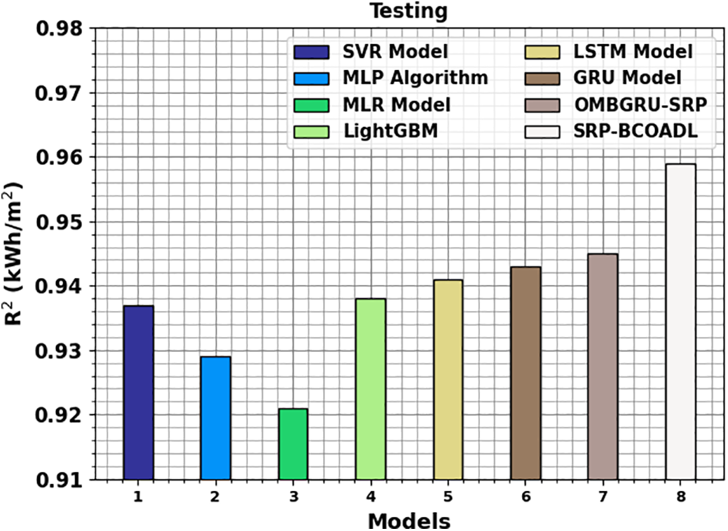
Figure 8: R2 outcome of SRP-BCOADL technique under testing set

A comparison study of the SRP-BCOADL system in terms of MSE is established in Fig. 9. The results pointed out that the SRP-BCOADL approach gets better performance with minimum values of MSE. It is perceived that the SRP-BCOADL method gains enhanced outcomes with least MSE of 0.132 kWH/m2 whereas the SVR, MLP, MLR, Light GBM, GRU, and OMBGRU-SRP methodologies have represented lesser MSE of 0.236, 0.264, 0.296, 0.233, 0.219, 0.193, and 0.169 kWH/m2, correspondingly.

Figure 9: MSE outcome of SRP-BCOADL technique under testing set

A comparison study of the SRP-BCOADL method in terms of RMSE is established in Fig. 10. The outcomes pointed out that the SRP-BCOADL method gets improved performance with minimum values of RMSE. It is perceived that the SRP-BCOADL model gets improved outcomes with a minimum RMSE of 0.363 kWH/m2 whereas the SVR, MLP, MLR, Light GBM, GRU, and OMBGRU-SRP techniques have represented lesser RMSE of 0.486, 0.514, 0.544, 0.483, 0.468, 0.440, and 0.412 kWH/m2, correspondingly.

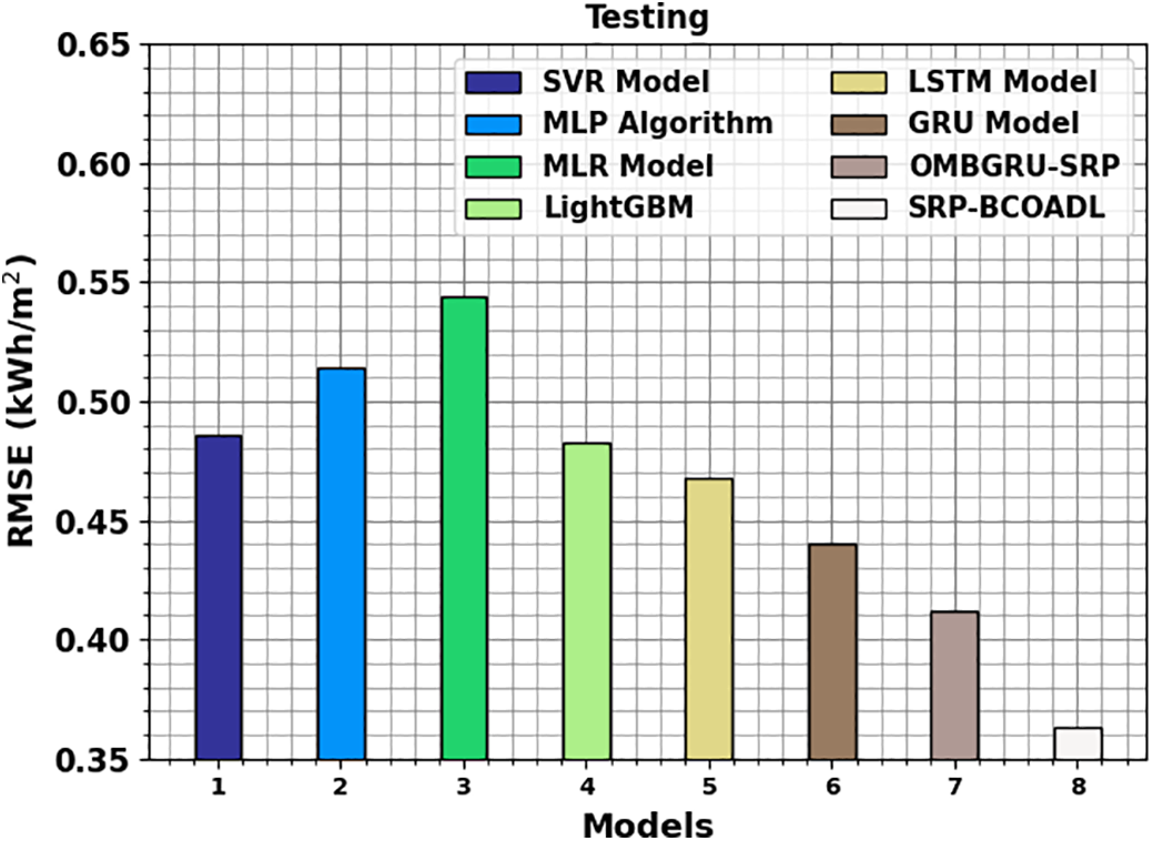
Figure 10: RMSE outcome of SRP-BCOADL technique under testing set

A comparison study of the SRP-BCOADL system in terms of MAE is established in Fig. 11. The results pointed out that the SRP-BCOADL method gets better performance with the smallest values of MAE. It is perceived that the SRP-BCOADL system gains upgraded outcomes with a minimum MAE of 0.279 kWH/m2 while the SVR, MLP, MLR, Light GBM, GRU, and OMBGRU-SRP techniques have described lower MAE of 0.392, 0.402, 0.361, 0.355, 0.348, 0.312, and 0.279 kWH/m2, individually.

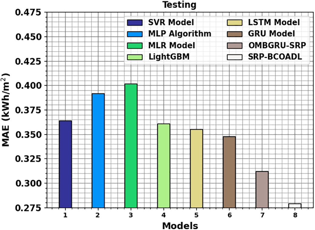
Figure 11: MAE outcome of SRP-BCOADL technique under testing set

Therefore, the SRP-BCOADL technique can be applied for improved prediction of solar radiation levels.

5  Conclusion

This paper presents a novel SRP-BCOADL model for energy forecasting. The SRP-BCOADL model employes three different processes namely data normalization, DLSTM-AE-based solar radiation prediction, and BCOA-based parameter selection. Initially, the technique applies min-max normalization to the input data to enhance robustness across varying data scales. The DLSTM-AE network is then utilized for accurate prediction of solar radiation levels. Performance evaluation on testing data demonstrates that the proposed model outperforms existing approaches. The Mean Squared Error is only 0.13 kWh/m2 which is much lower when compared to other models. The Root Mean Squared Error is also lower when compared to other models. The Mean Absolute Error is also at the lowest level of 0.276 kWh/m2. The effectiveness of the DLSTM-AE model can be improved by the design of a hyperparameter optimizer using BCOA. The performance analysis of the SRP-BCOADL technique is tested using solar radiation data. The extensive experimental outcomes show that the SRP-BCOADL method obtains high efficiency over other techniques under various measures. Deploying lightweight BCOA-DL models on IoT devices for applications like roof top solar and smart grid integration could prove invaluable for future studies. Additionally, embedding probabilistic layers within DL frameworks, guided by BCOA, can facilitate risk assessments to support critical decision-making in solar farm operations.

Acknowledgement: Not applicable.

Funding Statement: This research project was funded by the Deanship of Scientific Research and Libraries, Princess Nourah Bint Abdulrahman University, through the Program of Research Project Funding after Publication, grant No. (RPFAP-79-1445).

Author Contributions: Conceptualization: Shekaina Justin; Data Curation: Shekaina Justin; Methodology: Wafaa Saleh, Hind Mohammed Albalawi, J. Shermina, Shekaina Justin; Project administration: Wafaa Saleh, Hind Mohammed Albalawi, J. Shermina; Supervision: Wafaa Saleh, Hind Mohammed Albalawi, J. Shermina; Validation: Wafaa Saleh, Hind Mohammed Albalawi, J. Shermina; Writing—original draft: Shekaina Justin; Writing—review & editing: Wafaa Saleh, Hind Mohammed Albalawi, J. Shermina, Shekaina Justin. All authors reviewed the results and approved the final version of the manuscript.

Availability of Data and Materials: Data is contained within the article.

Ethics Approval: Not applicable.

Conflicts of Interest: The authors declare no conflicts of interest to report regarding the present study.

References

1. Hou M, Zhang T, Weng F, Ali M, Al-Ansari N, Mundher Yaseen Z. Global solar radiation prediction using hybrid online sequential extreme learning machine model. Energies. 2018;11(12):3415. doi:10.3390/en11123415. [Google Scholar] [CrossRef]

2. Ghimire S, Deo RC, Wang H, Al-Musaylh MS, Casillas-Pérez D, Salcedo-Sanz S. Stacked LSTM sequence-to sequence autoencoder with feature selection for daily solar radiation prediction: a review and new modeling results. Energies. 2022;15(3):1061. doi:10.3390/en15031061. [Google Scholar] [CrossRef]

3. Zhu T, Guo Y, Li Z, Wang C. Solar radiation prediction based on convolution neural network and long short-term memory. Energies. 2021;14(24):8498. doi:10.3390/en14248498. [Google Scholar] [CrossRef]

4. Ghimire S, Deo RC, Raj N, Mi J. Deep solar radiation forecasting with convolutional neural network and long short-term memory network algorithms. Appl Energy. 2019;253:113541. doi:10.1016/j.apenergy.2019.113541. [Google Scholar] [CrossRef]

5. Zhang Q, Tian X, Zhang P, Hou L, Peng Z, Wang G. Solar radiation prediction model for the yellow river basin with deep learning. Agronomy. 2022;12(5):1081. doi:10.3390/agronomy12051081. [Google Scholar] [CrossRef]

6. Han JM, Choi ES, Malkawi A. CoolVox: advanced 3D convolutional neural network models for predicting solar radiation on building facades. Build Simul. 2022;2(5):1081–768. doi:10.1007/s12273-021-0837-0. [Google Scholar] [CrossRef]

7. Reddy KN, Thillaikarasi M, Kumar BS, Suresh T. A novel elephant herd optimization model with a deep extreme learning machine for solar radiation prediction using weather forecasts. J Supercomput. 2022;78(6):8560–76. doi:10.1007/s11227-021-04244-y. [Google Scholar] [CrossRef]

8. Mukhtar M, Oluwasanmi A, Yimen N, Qinxiu Z, Ukwuoma CC, Ezurike B, et al. Development and comparison of two novel hybrid neural network models for hourly solar radiation prediction. Appl Sci. 2022;12(3):1435. doi:10.3390/app12031435. [Google Scholar] [CrossRef]

9. Zhu T, Li Y, Li Z, Guo Y, Ni C. Inter-hour forecast of solar radiation based on long short-term memory with attention mechanism and genetic algorithm. Energies. 2022;15(3):1062. doi:10.3390/en15031062. [Google Scholar] [CrossRef]

10. Huang H, Band SS, Karami H, Ehteram M, Chau KW, Zhang Q. Solar radiation prediction using improved soft computing models for semi-arid, slightly-arid and humid climates. Alex Eng J. 2022;61(12):10631–57. doi:10.1016/j.aej.2022.03.078. [Google Scholar] [CrossRef]

11. Waheed W, Xu Q. Data-driven short term load forecasting with deep neural networks: unlocking insights for sustainable energy management. Elect Power Syst Res. 2024;232(1):110376. doi:10.1016/j.epsr.2024.110376. [Google Scholar] [CrossRef]

12. Eşlik AH, Akarslan E, Hocaoğlu FO. Short-term solar radiation forecasting with a novel image processing-based deep learning approach. Renew Energy. 2022;200:1490–505. doi:10.1016/j.renene.2022.10.063. [Google Scholar] [CrossRef]

13. Quiñones JJ, Pineda LR, Ostanek J, Castillo L. Towards smart energy management for community microgrids: leveraging deep learning in probabilistic forecasting of renewable energy sources. Energy Convers Manag. 2023;293(4):117440. doi:10.1016/j.enconman.2023.117440. [Google Scholar] [CrossRef]

14. Sulaiman MH, Mustaffa Z. Forecasting solar power generation using evolutionary mating algorithm-deep neural networks. Energy AI. 2024;16(2):100371. doi:10.1016/j.egyai.2024.100371. [Google Scholar] [CrossRef]

15. Irshad K, Islam N, Gari AA, Algarni S, Alqahtani T, Imteyaz B. Arithmetic optimization with hybrid deep learning algorithm based solar radiation prediction model. Sustain Energy Technol Assess. 2023;57(4):103165. doi:10.1016/j.seta.2023.103165. [Google Scholar] [CrossRef]

16. Ghimire S, Deo RC, Casillas-Pérez D, Salcedo-Sanz S, Sharma E, Ali M. Deep learning CNN-LSTM-MLP hybrid fusion model for feature optimizations and daily solar radiation prediction. Measurement. 2022;202(7):111759. doi:10.1016/j.measurement.2022.111759. [Google Scholar] [CrossRef]

17. Ehteram M, Nia MA, Panahi F, Farrokhi A. Read-First LSTM model: a new variant of long short term memory neural network for predicting solar radiation data. Energy Convers Manag. 2024;305(9):118267. doi:10.1016/j.enconman.2024.118267. [Google Scholar] [CrossRef]

18. Ghimire S, Nguyen-Huy T, Prasad R, Deo RC, Casillas-Pérez D, Salcedo-Sanz S, et al. Hybrid convolutional neural network-multilayer perceptron model for solar radiation prediction. Cognit Comput. 2023;15(2):645–71. doi:10.1007/s12559-022-10070-y. [Google Scholar] [CrossRef]

19. Alkhatib FY, Alsadi J, Ramadan M, Nasser R, Awdallah A, Chrysikopoulos CV, et al. Comparative analysis of deep learning techniques for global horizontal irradiance forecasting in US cities. Clean Energy. 2025;9(2):2515–4230. doi:10.1093/ce/zkae097. [Google Scholar] [CrossRef]

20. Rajendran SS, Gebremedhin A. Deep learning-based solar power forecasting model to analyze a multi-energy microgrid energy system. Front Energy Res. 2024;12:1363895. doi:10.3389/fenrg.2024.1363895. [Google Scholar] [CrossRef]

21. Yadav AK, Kumar R, Wang M, Fekete G, Singh T. Comparative analysis of daily global solar radiation prediction using deep learning models inputted with stochastic variables. Sci Rep. 2025;15(1):10786. doi:10.1038/s41598-025-95281-7. [Google Scholar] [PubMed] [CrossRef]

22. Brahma B, Wadhvani R. Solar irradiance forecasting based on deep learning methodologies and multi-site data. Symmetry. 2020;12(11):1830. doi:10.3390/sym12111830. [Google Scholar] [CrossRef]

23. Mariappan Y, Ramasamy K, Velusamy D. An optimized deep learning based hybrid model for prediction of daily average global solar irradiance using CNN SLSTM architecture. Sci Rep. 2025;15(1):10761. doi:10.1038/s41598-025-95118-3. [Google Scholar] [PubMed] [CrossRef]

24. Jang SY, Oh BT, Oh E. A deep learning-based solar power generation forecasting method applicable to multiple sites. Sustainability. 2024;16(12):5240. doi:10.3390/su16125240. [Google Scholar] [CrossRef]

25. Wang Y, Luo Z, Kong Y, Luo J. Advancing spatiotemporal pollutant dispersion forecasting with an integrated deep learning framework for crucial information capture. Sustainability. 2024;16(11):4531. doi:10.3390/su16114531. [Google Scholar] [CrossRef]

26. Fahmi AT, Kashyzadeh KR, Ghorbani S. Fault detection in the gas turbine of the Kirkuk power plant: an anomaly detection approach using DLSTM-autoencoder. Eng Fail Anal. 2024;160(3):108213. doi:10.1016/j.engfailanal.2024.108213. [Google Scholar] [CrossRef]

27. Lan S, Razmjooy N. Enhancing the performance of zero energy buildings with boosted coyote optimization and elman neural networks. Energy Rep. 2024;11(21):5214–26. doi:10.1016/j.egyr.2024.05.001. [Google Scholar] [CrossRef]

28. Hasan SS, Agee ZS, Tahir BS, Zeebaree SR. Solar radiation prediction using satin bowerbird optimization with modified deep learning. Comput Syst Sci Eng. 2023;46(3):3225–38. doi:10.32604/csse.2023.037434. [Google Scholar] [CrossRef]

29. Chaibi M, Benghoulam EM, Tarik L, Berrada M, Hmaidi AE. An interpretable machine learning model for daily global solar radiation prediction. Energies. 2021;14(21):7367. doi:10.3390/en14217367. [Google Scholar] [CrossRef]