An Enhanced Image Classification Model Based on Graph Classification and Superpixel-Derived CNN Features for Agricultural Datasets

1  Introduction

In recent years, Artificial Intelligence (AI) has gained significant traction in agriculture, addressing challenges like crop disease identification, yield forecasting, and precision farming [1]. By leveraging technologies like deep learning, machine learning, computer vision, and automation is transforming traditional agricultural practices into data-driven systems. This shift enables real-time decision-making, enhances sustainability, optimizes the use of resources, and boosts productivity, while also addresses critical issues such as labor shortages, environmental impacts, and connectivity in modern agricultural operations [2]. One of the major challenges in modern agriculture is crop health monitoring. Early detection of plant diseases, nutrient deficiencies, and pest infestations is crucial to provide intervention solutions to ensure high yields [3]. Another important problem is automated fruit and vegetable grading, where AI-powered systems assess the quality of produce based on color, size, and texture [4]. Additionally, weed detection is a significant application where computer vision helps differentiate crops from weeds, reducing herbicide usage [5].

Image classification plays a fundamental role in solving many agricultural problems, including above issues. Modern AI models can analyze images of crops, leaves, fruits, and soil to classify plant conditions, detect diseases, and even assess plant growth stages [6]. This approach not only enhances efficiency but also enables real-time decision-making for farmers, contributing to the modernization of agriculture. Image classification tasks in agriculture are commonly implemented following two major approaches: (1) Image-level classification refers to the task of assigning a single label to an entire image. It is a fundamental problem in computer vision, where the objective is to categorize the whole image into one of predefined classes. (2) Pixel-level or region-based classification—assigning labels to groups of pixels or specific regions within an image and it is also known as semantic segmentation, involves classifying each pixel (or group of pixels) in an image into a specific class.

By leveraging both approaches, AI-based systems can offer scalable and precise solutions for wide range of agricultural applications, from disease detection and crop monitoring to quality assessment and resource optimization.

Traditional approaches of image classification typically adopt a two-step pipeline: First, handcrafted feature is extracted from an image, then this feature is passed into classifiers such as Support Vector Machines (SVM) or K-Nearest Neighbors (KNN) for final prediction. Among popular handcrafted feature descriptors, SIFT [7] is well-known due to its robustness to scale and rotation, while HOG [8] excels at capturing gradient-based texture patterns, which makes it effective for object detection problems. Despite their success in certain tasks, these methods heavily rely on manual feature engineering, which requires domain expertise and struggles to generalize well to large, diverse datasets. Second, with the advent of deep learning, particularly Convolutional Neural Networks (CNNs), the paradigm shifted from manual feature design to automatic hierarchical feature learning directly from raw image data. Early breakthroughs such as AlexNet [9], VGGNet [10], InceptionNet [11], and ResNet [12] have demonstrated the superior performance of deep CNNs over traditional methods in large-scale image classification tasks like ImageNet [13]. These models collectively shaped the evolution of CNN architectures, from increasing network depth and using smaller convolutional kernels to incorporating multi-scale feature extraction and residual learning. Kumar et al. [14] proposed a hybrid model combining Convolutional Auto-Encoder (CAE) and DenseNet-based CNN for automatic tomato leaf disease diagnosis without preprocessing, achieving 98.35% accuracy on the PlantVillage dataset with reduced training time due to fewer trainable components. Although CNNs achieve outstanding accuracy in many classification tasks, they also have limitations. CNNs inherently operate on regular grids of pixels, which may not fully capture irregular or non-Euclidean spatial structures present in some types of images, such as medical images or biological microscopy data. Additionally, deep CNNs demand large annotated datasets and considerable computational resources for training, which can be challenging in data-scarce or resource-constrained applications.

Overall, traditional handcrafted methods are simple and easy to interpret, but they lack flexibility and scalability. In contrast, CNN-based methods achieve much higher accuracy, especially on complex and large-scale image classification tasks, but they require more data and computational resources. Therefore, choosing the right method depends on the specific context and requirement of each classification problem. This limitation has motivated researchers to explore Graph Neural Networks (GNNs) as an alternative approach for image classification. GNNs are a family of deep learning models specifically designed to process graph-structured data, where data points are represented as nodes connected by edges [15]. Unlike traditional neural networks, which work on regular grids (like images) or sequences (like text), GNNs excel at modeling relationships in non-Euclidean spaces. This flexibility makes GNNs applicable to a wide range of tasks, including social network analysis, molecular property prediction, and image classification [16].

One of the main strengths of GNNs lies in their iterative aggregation of information from neighbor nodes, which allows the model to effectively captures both local structures and global dependencies within the graph. This capability is particularly beneficial in image classification, where understanding relationships between regions can enhance recognition accuracy. Among the various GNN architectures, Graph Convolutional Networks (GCNs) have gained widespread adoption due to their simplicity and effectiveness. GCNs extend the concept of convolution from CNNs to graph data by aggregating features from a node’s neighbors through a weighted sum [17]. In image classification tasks, this can be applied by first converting an image into a graph, where each node represents a meaningful region (e.g., pixel, superpixel) and edges encode spatial or semantic relationships between regions. This graph-based representation allows GCNs to integrate both local features and global context, offering a more holistic view of the image and improving classification performance. These two GCN-based approaches align closely with the two image classification paradigms discussed earlier: the first approach—graph-level classification—corresponds to assigning a single label to each image, while the second—node-level classification—corresponds to pixel-level or region-based classification, where each part of the image is individually labeled.

Although more recent architectures such as GraphSAGE [18] and GIN [19] have been proposed to address certain limitations of GCNs, GCN remains a preferred choice in many image classification applications due to its computational efficiency and stable performance on moderately sized graphs. GraphSAGE includes sampling strategies and more complex aggregation functions that are especially useful in large-scale or dynamic graphs, but may add unnecessary complexity when dealing with relatively static and structured graphs derived from images. Meanwhile, GIN achieves strong discriminative power by using multilayer perceptrons (MLPs) for aggregation, but often requires more extensive hyperparameter tuning and training resources. In contrast, GCNs provide a favorable trade-off between model expressiveness and computational simplicity, which makes them well-suited for tasks involving structured data such as images represented as graphs, especially when interpretability and efficiency are important [15,16].

Several studies applied GCNs to graph-level classification tasks, where each image was treated as a single graph to be labeled. Rodrigues et al. [20] conducted experiments on various image-to-graph transformation strategies including segmentation granularity, superpixel feature selection, and edge construction methods. Their experiments showed that these design choices substantially influence GCN performance. The best configuration yielded over 91.3 ± 0.4% accuracy across various datasets, confirming the feasibility and effectiveness of GCN-based models for image classification through graph representations. Han et al. [21] proposed Vision GNN (ViG), a novel graph-based architecture that represents images as graphs and achieved comparable accuracy to CNN-based ResNet models on CIFAR-10, while offering better interpretability due to its explicit graph structure. On the ImageNet dataset, ViG achieved 83.7% top-1 accuracy, and it also improved performance in object detection tasks on the COCO dataset, demonstrating strong representational capacity for both classification and detection tasks. Moreover, this study also demonstrated that the proposed method outperforms several other graph models, such as GraphSAGE and GIN.

In contrast, node-level classification is particularly effective for large-scale images (e.g., UAV (Unmanned Aerial Vehicle) imagery or hyperspectral images), which are divided into superpixels or patches. Each superpixel is modeled as a node, with edges capturing spatial or spectral relationships between them. GCNs are then used to label each node individually, enabling high-resolution, region-level interpretation. To support this, the miniGCN model proposed in [22] introduced an efficient mini-batch training scheme tailored for large-scale hyperspectral datasets. It also supports out-of-sample inference without retraining and integrates features from both CNNs and GCNs via various fusion strategies. Experiments on Indian Pines and Pavia University datasets showed significant improvements, with overall accuracy (OA) reaching 75.11% and 79.79%, respectively.

Another study [23] also leveraged multi-view features from hyperspectral images and applied GCNs to enhance classification performance by introducing an adaptive multi-feature fusion framework that integrates spectral and textural information through a multi-branch architecture with attention-based fusion. On the Salinas dataset, this method achieved an OA of 98.03 ± 1.02% and showed greater robustness to spectral variability, outperforming baseline CNNs by 4%–6% in overall accuracy. Liu et al. [24] introduced a CNN-enhanced GCN (CEGCN) that jointly learns from pixel- and superpixel-level features, integrating adaptive graph learning into the model. The proposed CEGCN was evaluated on three widely used hyperspectral image (HSI) datasets: Indian Pines, University of Pavia, and Salinas. Experimental results demonstrate that CEGCN consistently outperforms state-of-the-art deep learning methods (e.g., DCNN, HybridSN, and DBDA) in terms of OA, average accuracy (AA), and kappa coefficient (KPP). It effectively smooths predictions in homogeneous regions while preserving fine details in small or complex areas, and shows greater robustness under limited training data conditions. These studies collectively demonstrate the case-dependent performance of different GCN variants in image classification. While hybrid or enhanced models often outperform standard GCNs, the degree of improvement varies significantly across datasets—highlighting the importance of aligning model architecture with the structure and scale of the image data. Furthermore, GCNs remain a competitive baseline in many graph-based vision tasks due to their simplicity and reliability, particularly when interpretability and computational efficiency are key considerations.

In various studies on applying Graph Convolutional Networks (GCNs) for image classification problems, the first essential step is converting images from regular pixel grids into graph structures. One common approach represents each individual pixel as a node, with edges connecting neighboring pixel [25]. While this method preserves fine-grained spatial information, it results in extremely large and computationally expensive graphs, especially for high-resolution images. Another approach divides the image into uniform square patches, where each patch is treated as a node and edges link neighboring patches [21]. This reduces the graph size significantly, but it comes at the cost of losing important boundary details between objects, especially when object edges do not align with the patch boundaries.

To overcome these limitations, superpixel-based graph construction emerged as a more effective alternative. In this approach, the image is segmented into coherent regions—superpixels—that group together pixels with similar color, texture, or other low-level properties. Each superpixel becomes a node, and edges capture spatial relationships between neighboring superpixels [20,26]. This technique strikes a balance between reducing graph size and preserving important object boundaries and structural details, making it particularly suitable for image classification tasks where both local texture and global structure matter.

A key advantage of the superpixel-based graph construction method is the ability to balance graph complexity and structural preservation, which directly influences classification performance. Building on this foundation, several studies explored different strategies to optimize this approach, evaluated how various factors in graph construction impact the effectiveness of GCN models. One notable study, Rodrigue et al. [20] investigated different strategies for converting images into graphs, particularly by using superpixel segmentation. This research evaluates how various graph construction techniques impact classification performance, considering multiple aspects: the method of transforming an image into a graph, the number of nodes in the graph, the representation of features for each node, and the definition of edges between nodes. These factors play a crucial role in determining how well the graph structure preserves spatial and semantic relationships within the image, ultimately affecting the effectiveness of the GCN model. Similarly, Tang et al. [27] integrated the gSLIC superpixel algorithm with attention mechanisms, aiming to enhance GCNs’ ability to capture structural information within images. This study demonstrates that the proposed approach reduces graph construction time while also improving classification accuracy, making it a more efficient and effective method for image representation in GCN-based classification tasks.

Even though representing image as graph using superpixel-based segmentation proves to be a more suitable approach compared to the other two methods, thanks to it effectively balances computational efficiency and structural preservation. However, the next crucial challenge lies in determining the most effective way to define and represent node features for optimal classification performance. Rodrigue et al. [20] conducted experiments on seven different feature extraction methods and compared their effectiveness in GCN-based classification. These methods include spatial features such as the geometric centroid and pixel position distribution, structural features like the number of pixels per superpixel, and color-based features, including average RGB and HSV values along with their standard deviations. Their study emphasizes the significance of selecting appropriate node descriptors that not only capture local texture details but also preserve broader semantic information, ensuring that the graph representation retains essential characteristics for accurate image classification.

Another critical aspect of graph construction is constructing the connectivity between nodes, i.e., how edges are formed. In study [20], Rodrigue et al. explored three different strategies for establishing edges in superpixel-based graphs: Region Adjacency Graphs (RAGs), which connect nodes based on direct superpixel neighborhood relationships; K-Nearest Neighbors with spatial distance (KNN-Spatial), where nodes are linked to their closest neighbors based on spatial proximity; and K-Nearest Neighbors with combined spatial and color distances (KNN-Combined), which considers both spatial closeness and color similarity to form edges. Each of these approaches impacts how information propagates through the graph and influences the final performance of GCN models in classification tasks. Interestingly, their findings suggest that while more complex edge relationships, such as those incorporating both spatial and color distances, might intuitively capture richer structural information, they do not always lead to better classification performance. In some cases, simpler connectivity strategies, like RAGs or purely spatial KNN, are sufficient or even superior, highlighting the importance of carefully selecting edge construction methods based on the specific dataset and task requirements.

Building upon this foundation, this part of literature review focuses on how different published studies have implemented and applied graph-based models such as Graph Convolutional Networks (GCNs) to image-related tasks. We aim to examine the effectiveness of these approaches, analyzing the specific adaptations made to GCN architectures, the datasets used, and the overall impact on classification performance. By reviewing these implementations, we seek to gain deeper insights into the practical applications of GCNs in image classification and identify key factors that contribute to their success. In the study [27], Tang conducted a comprehensive analysis of graph-based classification methods using the GCN model. This study discussed key challenges, such as graph construction, over-smoothing, and scalability, while also explored strategies to overcome these issues. These studies highlight the importance of effective image-to-graph transformation and advanced graph processing techniques in leveraging GCNs for image classification.

Knyazev et al. [28] represented images as collections of superpixels and formulated the image classification task as a multigraph classification problem. This study extended graph convolution techniques and adopted relation type fusion methods to enhance the expressiveness of GCNs. To improve classification accuracy, they proposed a multigraph representation incorporating learnable and hierarchical relation types for a richer image representation. Through experiments were conducted on the MNIST, CIFAR-10, and PASCAL datasets, and their proposed model achieved notable improvements in accuracy, surpassing CNNs in specific classification tasks. Another significant work, Wharton et al. [29] proposed an innovative multi-scale hierarchical representation learning approach to enhance visual recognition. Additionally, they introduced a coarser hierarchical representation of multiple graphs using spectral clustering-based region aggregation. A novel gated attention mechanism was designed to aggregate cluster-level class-specific confidence. Their model was evaluated on five datasets covering fine-grained visual classification (FGVC) and generic visual classification, achieving competitive results.

As mentioned above, image classification is a core task in computer vision, serving as the foundation for a wide range of real-world applications. While Convolutional Neural Networks (CNNs) have achieved remarkable success in this domain, they have notable limitations. CNNs primarily operate on raw pixel grids, which restricts their ability to capture structural relationships between different image regions. Moreover, their reliance on dense pixel-level processing leads to high computational costs, making them inefficient for large-scale classification tasks.

To address these challenges, researchers have explored Graph Convolutional Networks (GCNs) as an alternative approach, leveraging graph structures to model spatial relationships within an image. In recent years, node-level classification using Graph Convolutional Networks (GCNs) has gained significant attention in the field of image classification, especially in applications involving high-resolution or structured data such as hyperspectral and UAV imagery. In this approach, each region or superpixel in an image is treated as a node in a graph, and the task is to assign a class label to each node. Numerous studies have demonstrated the effectiveness of GCNs in capturing spatial or spectral relationships between regions, thereby improving classification accuracy at the pixel or region level.

Despite these promising results, graph-level classification—where each entire image is represented as a graph and assigned a single label—remains relatively underexplored, particularly in the context of agricultural image analysis. This setting presents different challenges, such as how to construct graph representations that accurately reflect the holistic structure of an image and how to design models that can learn robust global features from such representations.

Motivated by the success of GCNs in node classification and the need for more scalable and generalizable models in agricultural tasks, this study shifts the focus toward graph-level classification. By representing each agricultural image as a graph and learning from the collective properties of its regions and their interrelations, we aim to explore the potential of GCNs in capturing global patterns and semantics that are critical for tasks such as crop type recognition or disease identification at the image level.

This study investigates the application of Graph Convolutional Networks (GCNs) for graph-level classification of agricultural images. While most existing works concentrate on node-level classification, this research focuses on the more challenging and less explored task of classifying entire images represented as graphs. The main contributions are as follows:

1.   Graph-Based Representation for Whole-Image Classification: We propose a framework that converts each image into a graph, enabling the application of GCNs to model spatial structures and semantic regions for comprehensive image classification.

2.   CNN-Based Node Feature Extraction Method: The study proposes a novel node feature extraction method that leverages a Convolutional Neural Network (CNN) to encode rich local visual patterns at the superpixel level. Each superpixel is passed through a lightweight CNN to obtain high-level features that are then used as node attributes in the graph.

3.   Application to Disease Classification and Ripeness Detection: The model is applied to two important agricultural tasks: plant disease classification and fruit ripeness detection, which shows the generalizability and effectiveness of the proposed graph-based representation method.

4.   Comparison with Cutting-Edge Deep Learning Models: The study performs a comprehensive comparison with other state-of-the-art models such as CNNs and Vision Transformers (ViTs). The experimental results demonstrate the superiority of our GCN-based approach in handling irregular and high-resolution agricultural images.

2  Preliminaries

2.1 Superpixels

Superpixels group similar pixels into meaningful regions, reducing data complexity while preserving image structure [30]. SLIC (Simple Linear Iterative Clustering) is a widely used superpixel method based on a modified k-means algorithm that clusters pixels by combining color similarity and spatial proximity [31]. The algorithm starts by dividing the image into a regular grid and placing initial cluster centers at low-gradient positions. Each pixel is then assigned to the nearest cluster using the distance D.

D=dc2+(dsS)2M2(1)

where dc is the color distance in CIELAB space, ds is the spatial distance, S is the superpixel size, and M controls compactness.

Clusters are iteratively refined by updating centers and reassigning pixels. A post-processing step merges small or disconnected regions to ensure spatial coherence. SLIC effectively preserves edges and reduces computational load, enabling region-based graph representations for improved performance in CNN and GNN-based image classification.

2.2 Convolutional Neural Networks (CNNs)

Convolutional Neural Networks (CNNs) are a type of deep learning model tailored for image processing [32], CNNs have established themselves as a cornerstone in contemporary computer vision applications, such as image classification, object detection, and segmentation. In contrast to traditional machine learning methods, CNNs are capable of automatically learning hierarchical features directly from raw image inputs, thereby minimizing the reliance on handcrafted feature extraction.

CNN Architecture

Convolutional Neural Networks (CNNs) are widely used deep learning models in image processing, consisting of convolutional layers, activation functions (typically ReLU), pooling layers, and fully connected layers. Convolutional layers use learnable kernels to extract visual features from input images. ReLU introduces non-linearity and helps mitigate the vanishing gradient problem. Pooling layers (commonly max pooling) reduce spatial dimensions, improving computational efficiency and generalization.

Over the years, CNN architectures have greatly advanced computer vision by improving depth, efficiency, and performance [32], such as AlexNet [9] introduced deeper networks with ReLU and dropout, leading to a major breakthrough. VGGNet [10] used small kernels to deepen networks, and ResNet [12] solved vanishing gradients with residual connections. EfficientNet [33] later optimized model scaling by balancing depth, width, and resolution. These innovations have enabled more powerful and scalable CNNs across vision tasks.

2.3 Graph Convolutional Networks

Graph Convolutional Networks (GCNs) are a type of deep learning model developed to handle graph-structured data, extending the capabilities of traditional Convolutional Neural Networks (CNNs) from Euclidean domains like images to non-Euclidean data, such as social networks, molecular structures, and citation graphs. Introduced by Kipf and Welling [17], GCNs leverage spectral graph theory and message-passing mechanisms to aggregate and update node features based on their neighbors’ information. This process consists of two key steps: message aggregation and feature update. At each layer, a node gathers feature information from its neighbors and combines it with its own features to learn a richer representation. Mathematically, this can be expressed as follows:

1.    Message Aggregation: Each node receives messages from its neighbors, which are typically weighted by a normalized adjacency matrix to ensure balanced contribution:

mv(l)=∑u∈𝒩(v)1|𝒩(v)|hu(l),(2)

where mv(l) represents the aggregated message for node v at layer l, hu(l) is a node feature of node u at layer l, and 𝒩(v) denotes the set of neighboring nodes.

2.   Feature Update: The node updates its representation using the aggregated messages and a transformation function:

hu(l+1)=σ(W(l)mv(l)+b),(3)

where W(l) is a trainable weight matrix, b is a bias term, and σ is a non-linear activation function like ReLU.

GCNs propagate information across the nodes of a graph through several convolutional layers. In each layer, a node’s features are updated by aggregating information from its neighboring nodes. This process enables the model to capture both local and global structural patterns within the graph. The steps involved include normalizing the adjacency matrix, aggregating the features from neighboring nodes, and applying a linear transformation followed by a non-linear activation function. This iterative process allows GCNs to refine node embeddings, which are crucial for tasks such as classification and segmentation.

Deeper GCN layers can capture higher-order dependencies, enhancing performance in relational tasks. However, too many layers may cause over-smoothing, making node features indistinguishable. To address this, techniques like residual connections and attention mechanisms are used to preserve expressive power and improve information flow.

Given an input graph with an adjacency matrix A and a feature matrix X, the forward propagation of a GCN layer is typically defined as:

H(l+1)=σ(D~−12A~D~−12H(l)W(l)),(4)

where A~=A+I is the adjacency matrix with self-loops added, I is the identity matrix, D~ is the degree matrix of A~, used for normalization. H(l) represents the node feature matrix at layer l, with H(0)=X being the initial node features. W(l) is the trainable weight matrix, and σ is a non-linear activation function. This formulation ensures that each node gathers information from its neighbors in a normalized manner, preventing scale imbalances and enabling effective learning of graph-based features, as illustrated in Fig. 1. By stacking multiple GCN layers, the network progressively captures higher-order dependencies, allowing for improved representation learning in various graph-structured tasks such as image classification, segmentation, and object recognition.

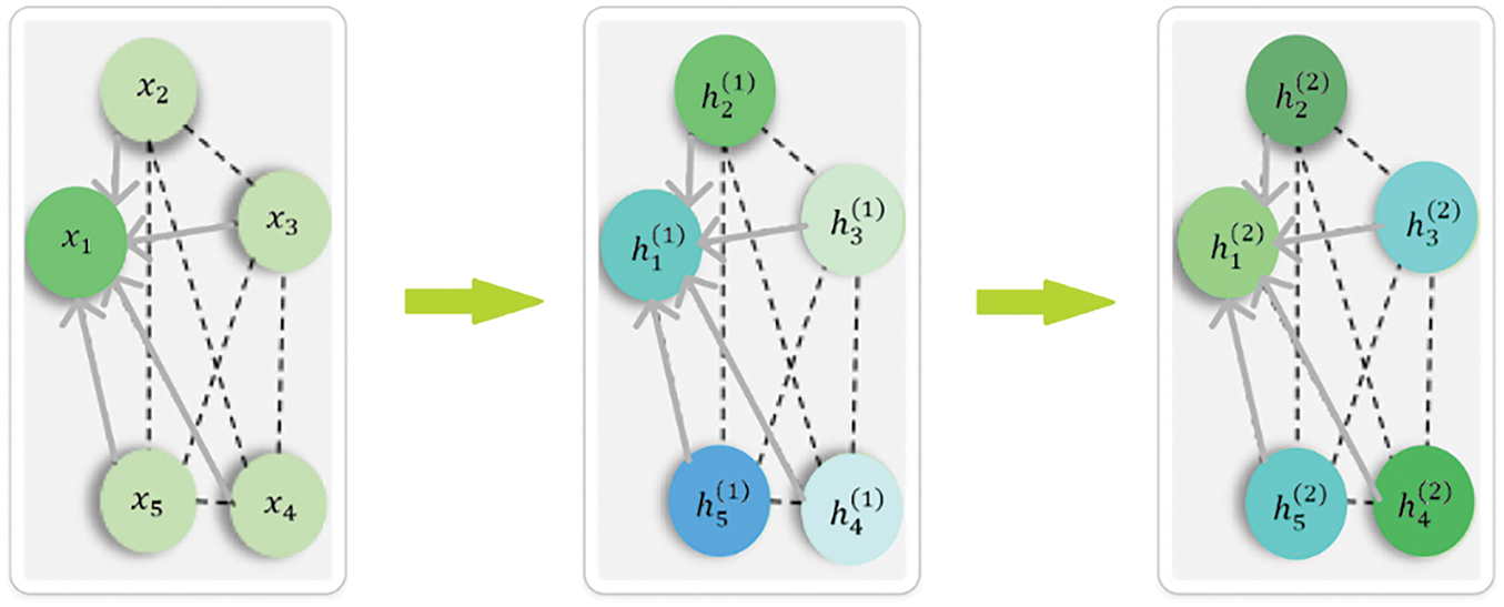
Figure 1: The feature aggregation mechanism of GCN

The number of GCN layers significantly impacts model performance. Unlike CNNs, deeper GCNs often face over-smoothing, where node features become indistinguishable. Studies [34–36] show that shallow GCNs (1–2 layers) work well for tasks relying on local information, like node classification. GCNs with 3–4 layers capture higher-order dependencies, suitable for complex graph structures such as image-based graphs. However, deeper GCNs (over 5 layers) lose expressiveness. To mitigate this, residual connections [37] and attention mechanisms [38,39] help maintain feature diversity. In image classification, research [40] suggests that 2–3 GCN layers offer a good trade-off between learning depth and avoiding over-smoothing, especially when combined with CNNs.

3  Proposed Graph Classification Model

In this section, the paper formally defines the problem addressed in this study, which is cast as a graph classification task—each agricultural image is treated as an individual graph, and the goal is to assign a corresponding class label to the entire graph. To enable this formulation, we first describe a graph construction methodology that transforms input images into graph representations by segmenting them into superpixels, defining nodes, extracting discriminative features, and establishing meaningful edge connections. The final subsection presents the proposed classification model, which employs a three-layer Graph Convolutional Network (GCN) to iteratively aggregate local node features and produce a robust graph-level representation for accurate classification.

3.1 Problem Definition

In this subsection, the problem considered within the scope of this study is defined. Specifically, we formulate the task as a graph classification problem, where each input image is represented as a graph and is associated with a corresponding label. This label may reflect certain semantic properties of the image, such as the type of crop disease or the ripeness level of a fruit.

Unlike node classification tasks, which assign labels to individual nodes within a graph, graph classification aims to predict a single label for the entire graph structure. The key challenge lies in effectively modeling the image as a graph in a way that preserves relevant spatial and contextual information. Let X and Y is images and labels set; dataset for classification tasks, D={(xi,yi)}i=1N where xi and yi is image and label ith. Each image xi transformed to graph Gi(V,E), where V, E present the sets of nodes and edges, respectively. Furthermore, each node vij∈V and edge eij∈E of the graph Gi carries features extracted from the original image xi, which encapsulate spatial, textural, or semantic information relevant to the classification task. These graph-structured representations allow the model to learn from both the local characteristics of image regions and their structural relationships within the image. The goal of image classification problems is translated into graph classification problems, f:G→Y.

In order to address the above image classification problem, this section presents an enhanced graph classification framework that amalgamates convolutional neural network (CNN) characteristics with a graph convolutional network (GCN) utilizing superpixel-based images. Fig. 2 shows details components of the proposed architecture. The proposed architecture consists of two main components: Graph Construction from Images detailed in Section 3.2 and a graph classification model for image classification present in Section 3.3.

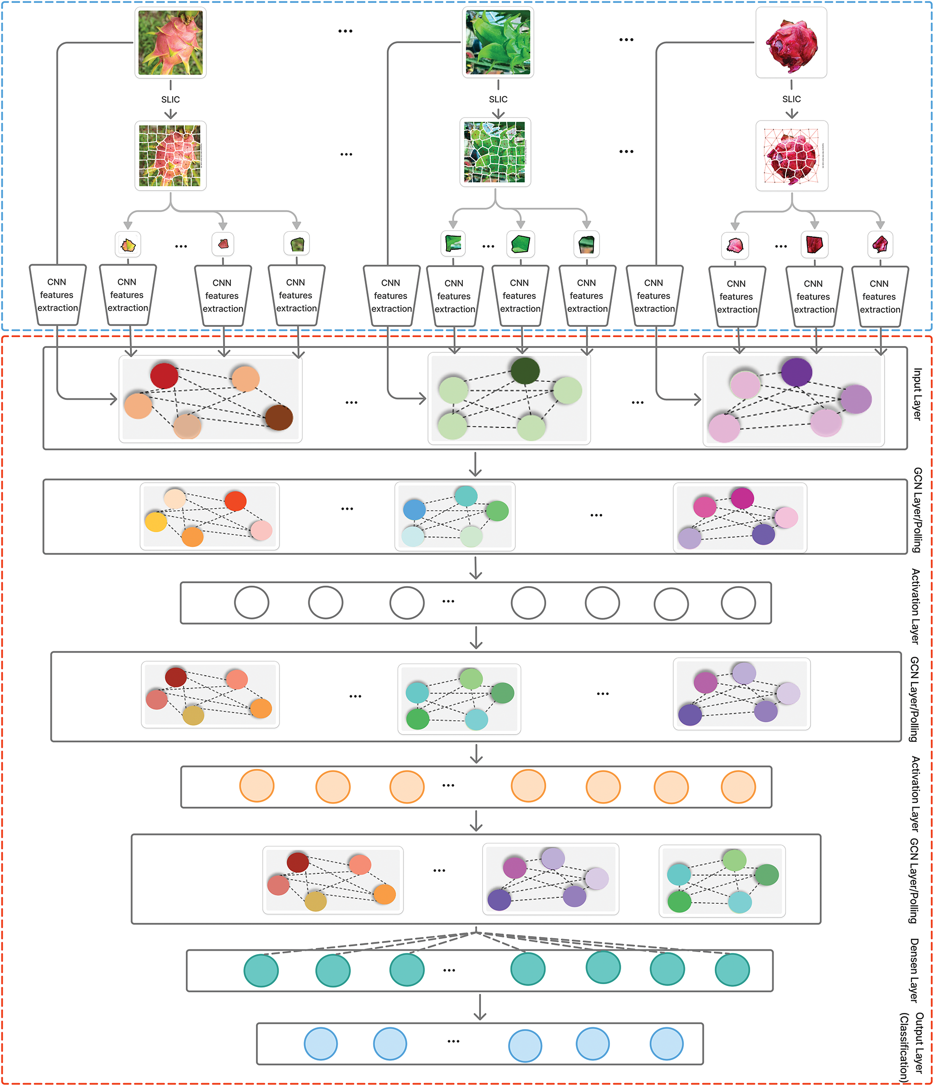
Figure 2: The proposed model for image classification problem

3.2 Graph Construction from Images

To construct a graph representation from a tomato leaf image, we follow a structured process where each superpixel serves as a node, and edges are formed based on spatial adjacency. The steps are as follows:

(1)   Superpixel Segmentation (Node Creation): The input image is first segmented into K superpixels using the SLIC algorithm. Each superpixel represents a meaningful region, that captures distinct parts of the leaf, such as veins, healthy areas, or diseased spots. These superpixels serve as nodes in a graph.

(2)   Node Feature Extraction: Each superpixel is represented by a feature vector extracted from a pretrained CNN model, such as ResNet50, VGG19, Inceptionv3, …, specifically, the superpixel region is resized to fit pretrained-CNN’s input size, and deep features are extracted from an intermediate layer of the network. The resulting feature vector serves as a node’s representation, ensuring that each node encodes high-level visual information, making it easier to distinguish between diseased and healthy regions.

(3)   Edge Construction Using RAG (Defining Node Relationships): In the Region Adjacency Graph (RAG) technique, edges are established based on spatial adjacency, meaning two nodes (superpixels) are connected if they share a boundary in the segmented image. This process involves constructing a graph where each node represents a superpixel, and edges capture the spatial relationships between them. The adjacency structure is encoded in an adjacency matrix A, where Aij=1 if nodes i and j are adjacent in the RAG, and Aij=0 otherwise. This graph-based representation preserves the structural integrity of the image while reducing computational complexity, making it highly effective for tasks such as image classification and segmentation. The image graph is illustrated in Fig. 3.

(4)   Graph Representation: After defining nodes as superpixels with Pretrained CNN features and edges as adjacency relationships, the leaf image is represented as an undirected graph G=(V,E), where V is the set of superpixel nodes with feature vectors from pretrained model, such as ResNet50, VGG19, Inceptionv3, …, and E is the set of edges preserving the spatial structure of the image. This graph structure is then fed into a Graph Convolutional Network (GCN) for classification, enabling the model to leverage both local superpixel features and global structural relationships for improved disease recognition.

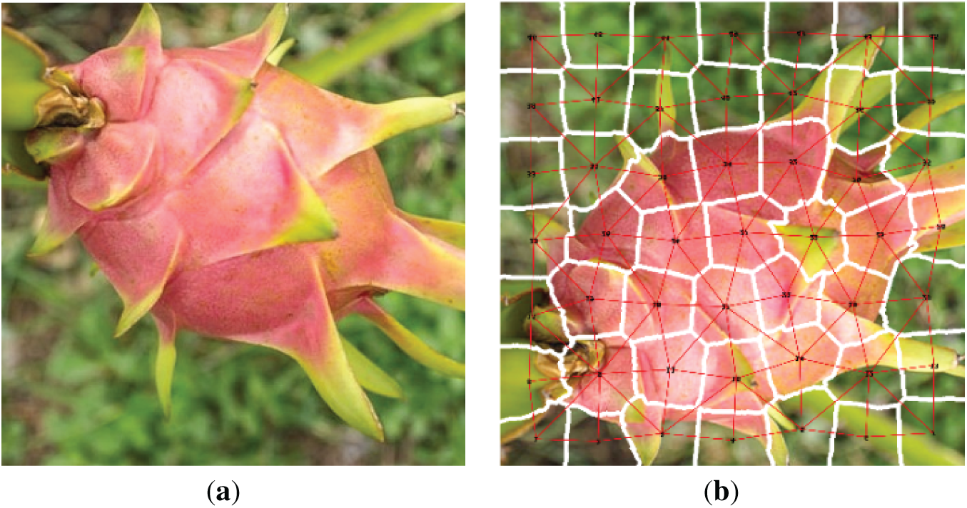
Figure 3: The image is converted into a graph using the RAG technique. (a) Raw; (b) Superpixcel

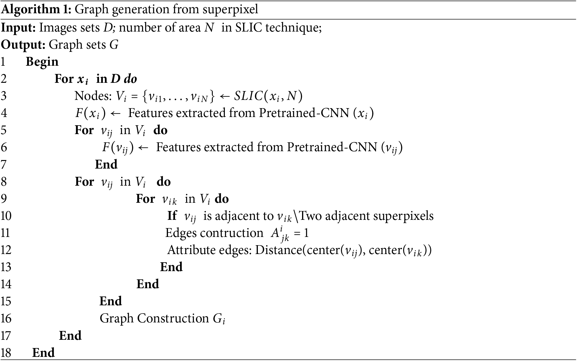
The algorithm for constructing a graph from the original image using the superpixel technique is described as follows (Algorithm 1).

3.3 Graph Classification Model for Image Classification

In this subsection, we present the proposed GCN classification model for graph-based image classification. The details of the proposed model are shown in Fig. 2. The proposed model comprises three principal components, the following:

(1)   Input layer: This layer in the proposed model preprocesses the graph-structured data, which typically includes node features, adjacency matrices, and edge attributes. The detailed steps for constructing graphs from images are presented in Section 3.2. This stage involves normalizing features, partitioning the graph into training, test sets while preserving structural dependencies.

(2)    Hidden layers: This layer consists of three graph convolutional layers (GCNConv) and a fully connected linear layer for final classification. We chose to use three GCN layers as they strike a balance between capturing local dependencies within the graph and avoiding over-smoothing, where node features can become indistinguishable after too many layers. This choice is crucial for preserving feature distinctiveness while learning global representations of the image. The input node features are passed through three consecutive GCN layers, each followed by a ReLU activation function to introduce non-linearity. These layers progressively capture structural relationships between nodes, with each layer learning increasingly abstract features while maintaining local context. The model also applies a global mean pooling operation that aggregates the node embeddings into a single graph-level representation. This step is essential for classification tasks where the entire graph represents an image, ensuring that information from all regions of the image is effectively combined. In the first GCN layer, node features are reduced from 1035 dimensions—extracted from the previously discussed feature extraction model—to 64 dimensions. The subsequent two GCN layers maintain this 64-dimensional representation, allowing the model to progressively refine the features while preserving the structural and contextual information within the graph.

(3)   Output layer: The model applies a dropout layer with a probability of 0.5 to prevent overfitting, followed by a fully connected linear layer that maps the extracted features to the final output classes.

The proposed model would be trained using standard classification loss functions such as cross-entropy loss, helping the model learn to assign the correct class to the input graph. By using three GCN layers, we ensure efficient learning of both local and global features without overcomplicating the model, resulting in optimal performance in image classification tasks.

3.4 Computational Complexity Evaluation

To evaluate the computational complexity of the model, it is necessary to consider two separate components: (1) the computational complexity of the image-to-graph conversion and feature extraction using ResNet50, and (2) the computational complexity of the GCN model. Assume the number of images is M, and the number of superpixels per image is N. The computational complexity of SLIC is O(SLIC), while feature extraction via CNN is O(CNNfull) for the entire image and O(CNNpatch) for each superpixel. Based on Algorithm 1, the computational complexity of converting the image dataset into graphs is O(M×[SLIC+CNNfull+N×CNNpatch+N2]). From Eq. (4), the computational complexity of the GCN is given by O(|E|×Fl×Fl+1+|N|×Fl+1) where |E| is the number of edges, Fl and Fl+1 are input and output feature dimensions respectively, and N is the number of nodes. The complexity of GCNs primarily depends on the number of nodes and edges, which is determined by the graph’s sparsity. In our experiments, the constructed graphs are relatively small, typically consisting of around 100 nodes. Edges are only formed between adjacent superpixels, resulting in sparse graphs with an average node degree of 3–4. In contrast, the computational complexity of CNNs is heavily influenced by image resolution and network depth—particularly in deep architectures like ResNet or VGG. Compared to these CNN models, the proposed GCN demonstrates significantly lower computational complexity due to its compact and sparse graph structure. However, the image-to-graph conversion step introduces an additional computational cost of the image-to-graph conversion O(M×[SLIC+CNNfull+N×CNNpatch+N2]).

4  Experiments and Analysis

4.1 Datasets

In this subsection, the paper conducted experiments on four datasets with different image quantities, class distributions, and resolutions to evaluate whether the proposed model is suitable for various classification tasks.

•   Dataset 1. The Tomato Leaf dataset from Kaggle [41], which includes 10 different disease types. This dataset helps evaluate the model’s ability to detect and classify plant diseases, which is crucial for precision agriculture and early disease management.

•   Dataset 2. Classification of the ripeness stages (green, ripe, and rotten) of dragon fruit. This dataset is important for automated fruit quality assessment, aiding in post-harvest processing and reducing food waste.

•   Dataset 3. Classification of the ripeness levels of tomatoes. This task focuses on determining different ripeness stages, which are essential for supply chain optimization, harvesting decisions, and market readiness assessment. The dataset used for this task was collected directly by the authors from real-world sources, including tomato gardens and supermarkets. The images were simply processed through cropping and resizing, while retaining the original background and complex real-world contexts. This ensures a more realistic evaluation of model performance in practical scenarios, where environmental noise and varied backgrounds are present.

•   Dataset 4. Classification of dragon fruit and leaf images. This task focuses on distinguishing between fruit and leaf instances, which is essential for automated plant monitoring, disease detection, and improving agricultural decision-making processes.

The details of the four datasets are presented in Table 1.

4.2 Experiments

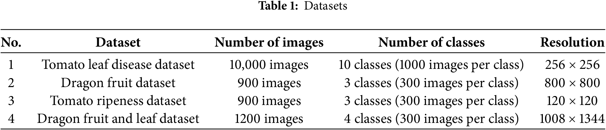
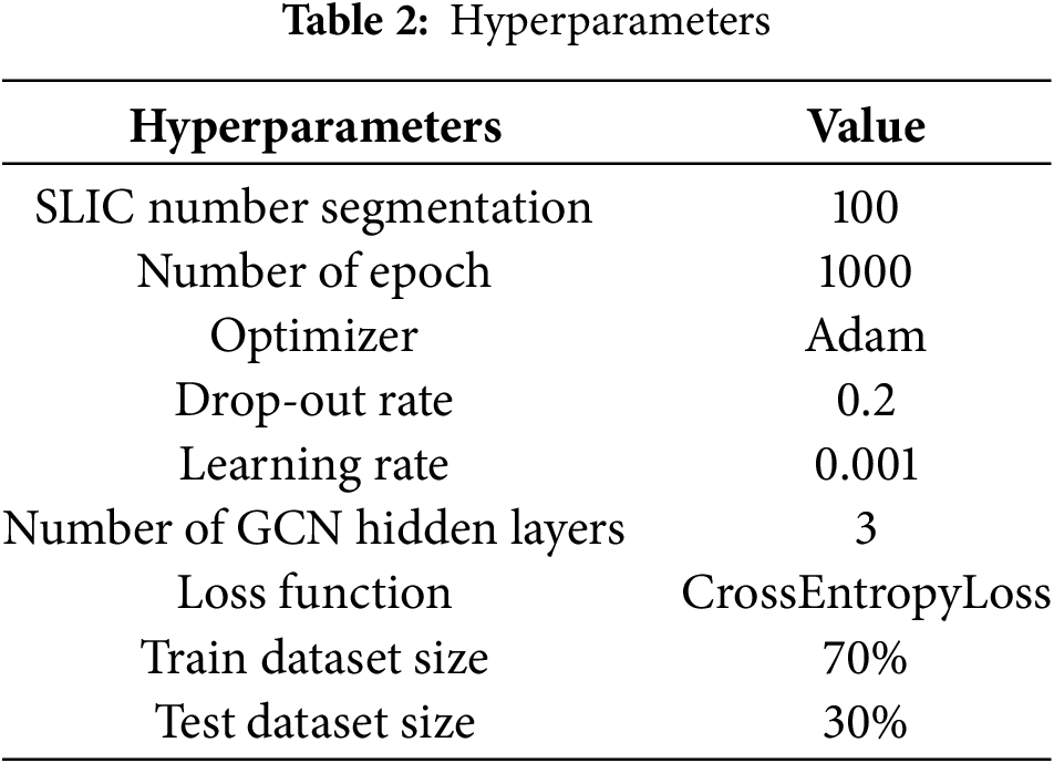
Table 2 shows hyperparameter’s details of the proposed model. All experiments were ran in a computer with a NVIDIA Geforce RTX 3050, 8 GB of RAM.

The following results were obtained: Fig. 4 illustrates the learning process, and the loss function values for each dataset. Table 3 and Fig. 5 show classification results of the proposed model across four agricultural image datasets. The metrics of accuracy, precision, recall, F1-score, and the results from the confusion matrix exhibit elevated values, thereby indicating that the proposed model showcases robust classification performance across four datasets.

Figure 4: Example of loss function Values on two datasets. (a) Tomato leaf disease dataset; (b) Dragon fruit dataset

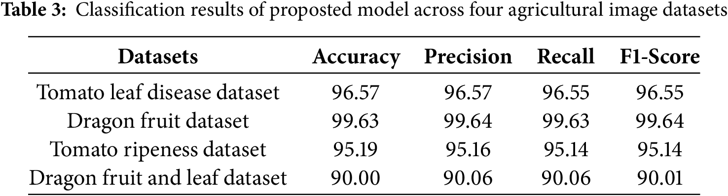
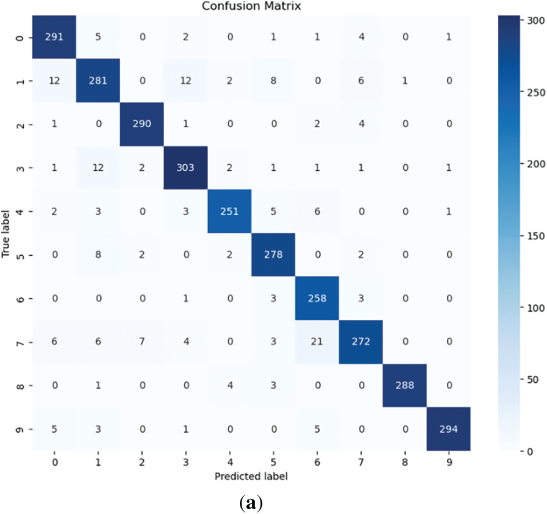
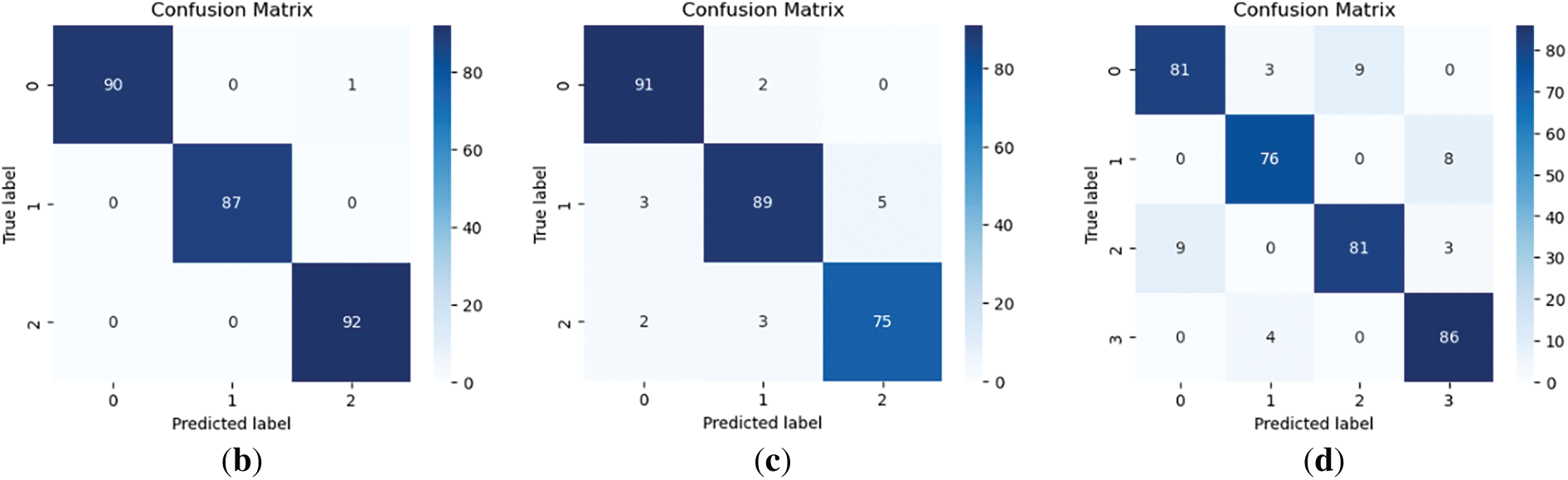
Figure 5: Confusion matrix. (a) Tomato leaf disease dataset; (b) Dragon fruit dataset; (c) Tomato ripeness dataset; (d) Dragon fruit and leaf dataset

4.3 Comparative Analysis

To assess the performance of the proposed model, this section compares the model against four representative traditional deep learning architectures, such as, CNN, ViT, ResNet50, and VGG16. The Convolutional Neural Network (CNN) is a foundational model in image classification, known for its ability to effectively extract local spatial features through stacked convolutional and pooling layers. The Vision Transformer (ViT) represents a transformer-based approach that divides an image into patches and applies self-attention to model global contextual information, making it suitable for capturing long-range dependencies. ResNet50, a deep residual network, enhances training stability and depth scalability by introducing identity shortcut connections, enabling efficient learning in very deep architectures. VGG16 is a classic convolutional architecture that employs a deep stack of small (3 × 3) convolution filters, offering simplicity and effectiveness for image classification tasks. In addition, our proposed GCN-based model, previously described in detail, leverages superpixel segmentation and node-level feature aggregation to perform graph-based image classification. This comparative setup allows for a comprehensive evaluation across diverse model paradigms.

Table 4 shows the experimental results of comparing models on four datasets. The experimental result presented in the table reveals several key observations regarding model performance across different agricultural image classification tasks. Overall, the proposed model consistently achieves competitive and often superior accuracy compared to conventional deep learning models.

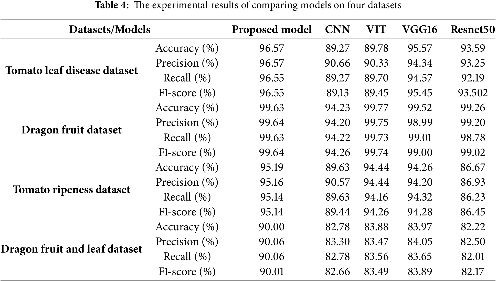
•   On the Tomato Leaf Disease Dataset, the Proposed Model achieves a strong performance (96.57%), slightly behind VGG16 (95.57%) but clearly outperforming CNN (89.27%), ViT (89.78%), and ResNet50 (93.59%). This demonstrates the model’s effectiveness in identifying disease patterns.

•   For the Dragon Fruit Dataset, ViT leads with the highest accuracy (99.77%), but the Proposed Model performs nearly as well (99.63%), surpassing VGG16 (99.52%) and ResNet50 (99.26%). CNN again shows weaker performance (94.23%).

•   In the Tomato Ripeness Dataset, the Proposed Model outperforms all other models with 95.19% accuracy, followed by ViT (94.44%) and VGG16 (94.26%). ResNet50 has the lowest score (86.67%), suggesting it is less suitable for this task.

•   On the Dragon Fruit and Leaf Dataset, the Proposed Model achieves the highest accuracy (90.00%), significantly outperforming CNN (82.78%), ViT (83.88%), VGG16 (83.97%), and ResNet50 (82.22%), highlighting its robustness in complex, multi-class scenarios.

These results highlight the robustness and the generalizability of the proposed model, particularly in cases where spatial relationships between regions (e.g., superpixels) are crucial. While traditional models like VGG16 and ViT perform well in certain datasets, GCN demonstrates more consistent performance across varied tasks, making it a promising approach for complex agricultural image classification problems.

The other four datasets also achieve very high accuracy, demonstrating that the proposed model is well-suited for various datasets with different resolutions. This suggests that the graph-based representation effectively captures essential image features across diverse image sizes and structures, making it a versatile approach for image classification tasks.

The experimental results indicate that the proposed model achieves high performance across various agricultural image classification tasks. Notably, on the Dragon Fruit Dataset, the model obtains the highest evaluation metrics, with accuracy, precision, recall, and F1-score all exceeding 99%, suggesting strong effectiveness when distinguishing between clearly defined classes. For the Tomato Leaf Disease and Tomato Ripeness datasets, the model also demonstrates robust performance, achieving accuracies of 96.57% and 95.19%, respectively. These results highlight the model’s ability to handle more challenging classification tasks involving subtle variations in disease symptoms or fruit maturity. The Dragon Fruit and Leaf Dataset presents a more complex scenario, with lower performance (accuracy: 90.00%). This may be due to the visual similarities between fruit and leaf regions, which can make classification more difficult. Nevertheless, the model maintains a relatively high level of performance. Overall, these findings demonstrate the generalizability and effectiveness of the model across different agricultural image classification scenarios.

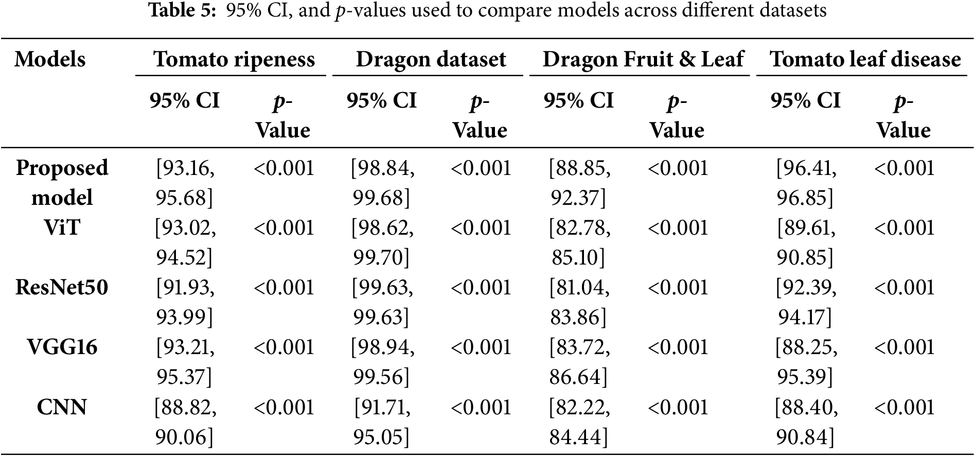
Table 5 shows the accuracy, 95% confidence intervals, and p-values for the proposed model compared with ViT, ResNet50, VGG16, and CNN across four different agricultural datasets. The proposed model consistently outperforms other baselines, particularly in complex datasets such as Dragon Fruit & Leaf and Tomato Leaf Disease, where the performance gap is substantial. All p-values are less than 0.001, indicating statistically significant differences between the models. These results indicate that the proposed model achieves accuracy comparable to CNNs while significantly reducing input size, thereby lowering computational complexity. The input sizes for the three datasets are detailed in Table 6, highlighting the efficiency of the graph-based representation in contrast to raw pixel-based inputs.

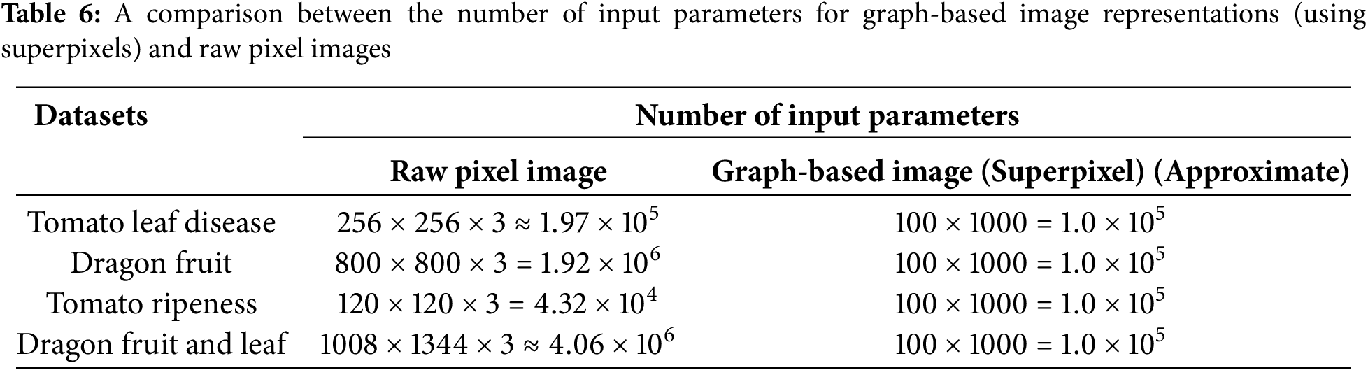
For example, an image with a resolution of 256 × 256 and three color channels (RGB) have 256 × 256 × 3 = 196,608 input parameters for a raw pixel representation. In contrast, after superpixel segmentation (say 100 superpixels), each superpixel represents a node, and the input size would be reduced to 100× features per node. The reduction in input size leads to more computational efficiency, allowing the model to focus on more abstract features rather than low-level pixel values.

4.4 Interpretability Analysis

Although our model does not incorporate attention mechanisms, we analyze the importance of individual nodes to provide insight into the decision-making process. Fig. 6 shows the distribution of node importance scores, where only a few nodes exhibit significantly high contributions while most remain near zero. This suggests that the model focuses on a sparse subset of the graph during classification. Fig. 7 highlights the top 20 most important nodes, further illustrating which parts of the graph drives the final prediction. This interpretability approach offers an alternative perspective similar to attention visualization in transformer-based models.

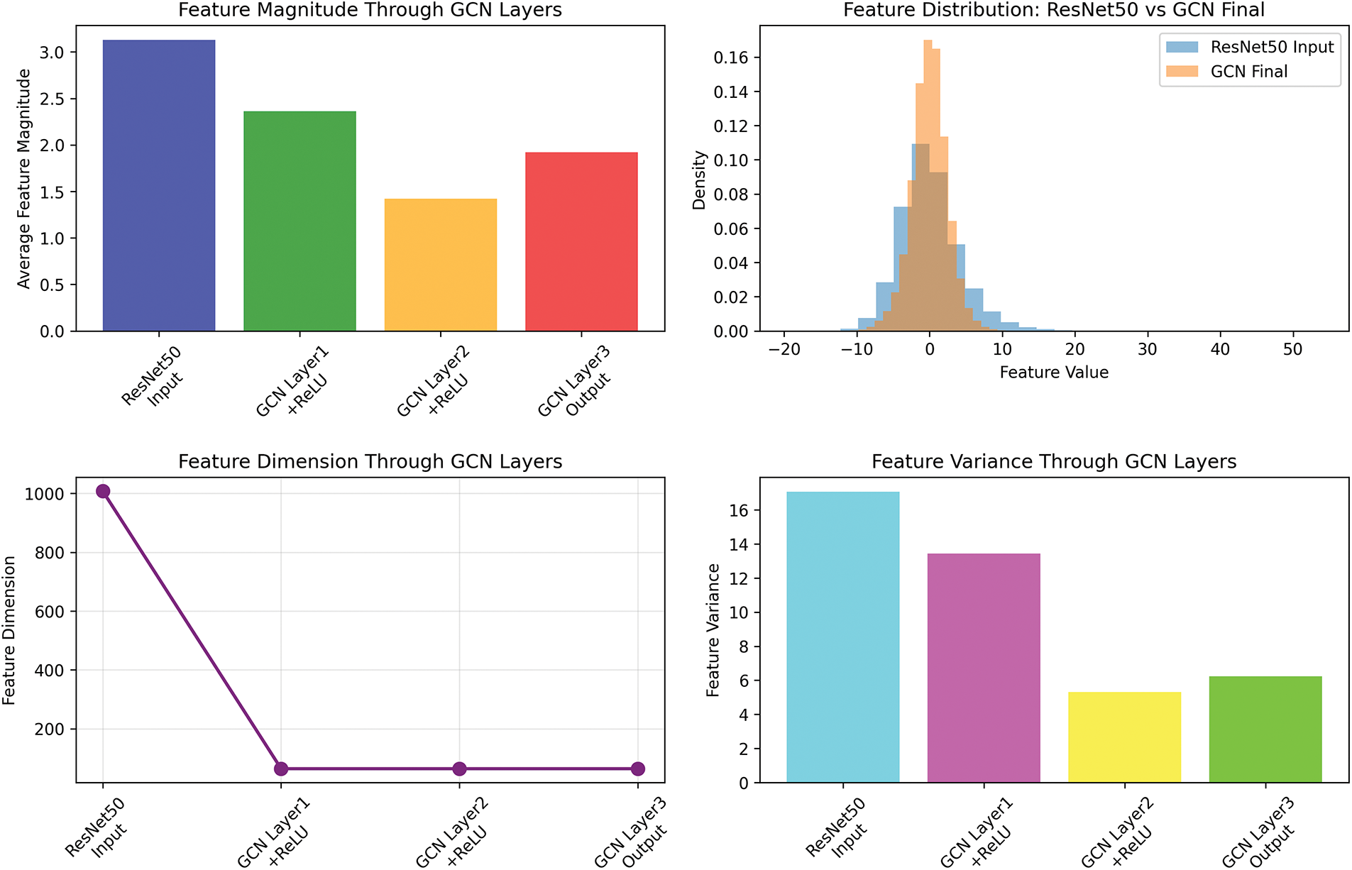
Figure 6: Distribution of importance scores across all nodes shows that only a few nodes significantly contribute to the final prediction

Figure 7: Top 20 most important nodes ranked by their contribution scores

5  Conclusions

In this study, we explored the effectiveness of Graph Convolutional Networks (GCNs) for image classification by leveraging superpixel-based graph representations. This task is crucial for many AI-based applications in modern agricultural models. While traditional CNNs have shown great success in this domain, they often require large computational resources due to their reliance on raw pixel data. By transforming images into graph structures, our proposed approach significantly reduces input size while maintaining high classification accuracy. Experimental results across multiple datasets demonstrate that the proposed method performs competitively with CNNs, achieving high accuracy even with reduced input complexity. The findings suggest that superpixel-based graph representations effectively capture spatial relationships within an image, enabling GCNs to extract meaningful features while minimizing computational costs. Moreover, our comparative analysis highlights the trade-offs between raw pixel-based CNNs and graph-based learning. While CNNs operate directly on pixel grids, GCNs benefit from structured feature learning, which enhances classification performance without excessive computational overhead. The success of our model across different datasets indicates its adaptability to various image resolutions and domains.

Although this study evaluated the proposed model on diverse set of agricultural image datasets, we acknowledge that the current evaluation does not fully validate the model’s generalization ability under more complex real-world conditions. Specifically, scenarios involving occlusions, lighting variations, and cluttered or dynamic backgrounds are underrepresented in the existing datasets. Therefore, an important future research direction is to collect more challenging datasets that better reflect such complexities. This would enable a more rigorous assessment of the model’s robustness and adaptability in practical agricultural applications.

Overall, our study underscores the potential of graph-based learning as a promising alternative to conventional deep learning methods in image classification. Future work can focus on optimizing graph construction techniques, exploring hybrid models that integrate CNN-based feature extraction with GCN-based relational learning, and extending the approach to more complex real-world applications.

Acknowledgement: Not applicable.

Funding Statement: This research is funded by Thuongmai University, Hanoi, Vietnam.

Author Contributions: The authors confirm contribution to the paper as follows: study conception and design: Tho Thong Nguyen, Thi Phuong Thao Nguyen, Huu Quynh Nguyen, Nguyen Giap Cu; data collection: Tien Duc Nguyen, Chu Kien Nguyen; software development: Tien Duc Nguyen, Chu Kien Nguyen; analysis and interpretation of results: Thi Phuong Thao Nguyen, Tho Thong Nguyen; draft manuscript preparation: Thi Phuong Thao Nguyen, Tho Thong Nguyen, Nguyen Giap Cu. All authors reviewed the results and approved the final version of the manuscript.

Availability of Data and Materials: The data that support the findings of this study are available from the corresponding author upon reasonable request.

Ethics Approval: Not applicable.

Conflicts of Interest: The authors declare no conflicts of interest to report regarding the present study.

References

1. Albahar M. A survey on deep learning and its impact on agriculture: challenges and opportunities. Agriculture. 2023;13(3):540. doi:10.3390/agriculture13030540. [Google Scholar] [CrossRef]

2. Vinod Chandra SS, Anand Hareendran S, Albaaji GF. Precision farming for sustainability: an agricultural intelligence model. Comput Electron Agric. 2024;226(1):109386. doi:10.1016/j.compag.2024.109386. [Google Scholar] [CrossRef]

3. Demilie WB. Plant disease detection and classification techniques: a comparative study of the performances. J Big Data. 2024;11(1):5. doi:10.1186/s40537-023-00863-9. [Google Scholar] [CrossRef]

4. Rizzo M, Marcuzzo M, Zangari A, Gasparetto A, Albarelli A. Fruit ripeness classification: a survey. Artif Intell Agric. 2023;7(2):44–57. doi:10.1016/j.aiia.2023.02.004. [Google Scholar] [CrossRef]

5. Vasileiou M, Kyrgiakos LS, Kleisiari C, Kleftodimos G, Vlontzos G, Belhouchette H, et al. Transforming weed management in sustainable agriculture with artificial intelligence: a systematic literature review towards weed identification and deep learning. Crop Prot. 2024;176:106522. doi:10.1016/j.cropro.2023.106522. [Google Scholar] [CrossRef]

6. Ferentinos KP. Deep learning models for plant disease detection and diagnosis. Comput Electron Agric. 2018;145(6):311–8. doi:10.1016/j.compag.2018.01.009. [Google Scholar] [CrossRef]

7. Lowe DG. Distinctive image features from scale-invariant keypoints. Int J Comput Vis. 2004;60(2):91–110. doi:10.1023/B:VISI.0000029664.99615.94. [Google Scholar] [CrossRef]

8. Dalal N, Triggs B. Histograms of oriented gradients for human detection. In: 2005 IEEE Computer Society Conference on Computer Vision and Pattern Recognition (CVPR’05); 2005 Jun 20–25; San Diego, CA, USA. p. 886–93. doi:10.1109/CVPR.2005.177. [Google Scholar] [CrossRef]

9. Krizhevsky A, Sutskever I, Hinton GE. ImageNet classification with deep convolutional neural networks. Commun ACM. 2017;60(6):84–90. doi:10.1145/3065386. [Google Scholar] [CrossRef]

10. Simonyan K. Very deep convolutional networks for large-scale image recognition. arXiv:1409.1556. 2014. doi:10.48550/arXiv.1409.1556. [Google Scholar] [CrossRef]

11. Szegedy C, Liu W, Jia Y, Sermanet P, Reed S, Anguelov D, et al. Going deeper with convolutions. In: 2015 IEEE Conference on Computer Vision and Pattern Recognition (CVPR); 2015 Jun 7–12; Boston, MA, USA. doi:10.1109/CVPR.2015.7298594. [Google Scholar] [CrossRef]

12. He K, Zhang X, Ren S, Sun J. Deep residual learning for image recognition. In: 2016 IEEE Conference on Computer Vision and Pattern Recognition (CVPR); 2016 Jun 27–30; Las Vegas, NV, USA. p. 770–8. doi:10.1109/CVPR.2016.90. [Google Scholar] [CrossRef]

13. Deng J, Dong W, Socher R, Li LJ, Kai L, Li FF. ImageNet: a large-scale hierarchical image database. In: 2009 IEEE Conference on Computer Vision and Pattern Recognition; 2009 Jun 20–25; Miami, FL, USA. p. 248–55. doi:10.1109/CVPR.2009.5206848. [Google Scholar] [CrossRef]

14. Kumar T, Kaur S, Sharma P, Chhikara A, Cheng X, Lalar S, et al. Plant disease detection and classification using hybrid model based on convolutional auto encoder and convolutional neural network. Comput Mater Contin. 2025;83(3):5219–34. doi:10.32604/cmc.2025.062010. [Google Scholar] [CrossRef]

15. Wu Z, Pan S, Chen F, Long G, Zhang C, Yu PS. A comprehensive survey on graph neural networks. IEEE Trans Neural Netw Learning Syst. 2021;32(1):4–24. doi:10.1109/tnnls.2020.2978386. [Google Scholar] [PubMed] [CrossRef]

16. Zhou J, Cui G, Hu S, Zhang Z, Yang C, Liu Z, et al. Graph neural networks: a review of methods and applications. AI Open. 2020;1(1):57–81. doi:10.1016/j.aiopen.2021.01.001. [Google Scholar] [CrossRef]

17. Kipf TN, Welling M. Semi-supervised classification with graph convolutional networks. arXiv:1609.02907. 2016. doi:10.48550/arXiv.1609.02907. [Google Scholar] [CrossRef]

18. Hamilton W, Ying Z, Leskovec J. Inductive representation learning on large graphs. arXiv:1706.02216. 2017. doi:10.48550/arXiv.1706.02216. [Google Scholar] [CrossRef]

19. Xu K, Hu W, Leskovec J, Jegelka S. How powerful are graph neural networks? arXiv:1810.00826. 2018. doi:10.48550/arXiv.1810.00826. [Google Scholar] [CrossRef]

20. Rodrigues J, Carbonera J. Graph convolutional networks for image classification: comparing approaches for building graphs from images. In: Proceedings of the 26th International Conference on Enterprise Information Systems; 2024 Apr 28–30; Angers, France. p. 437–46. doi:10.5220/0012263200003690. [Google Scholar] [CrossRef]

21. Han K, Wang Y, Guo J, Tang Y, Wu E. Vision GNN: an image is worth graph of nodes. arXiv:2206.00272. 2022. doi:10.48550/arXiv.2206.00272. [Google Scholar] [CrossRef]

22. Hong D, Gao L, Yao J, Zhang B, Plaza A, Chanussot J. Graph convolutional networks for hyperspectral image classification. IEEE Trans Geosci Remote Sens. 2021;59(7):5966–78. doi:10.1109/TGRS.2020.3015157. [Google Scholar] [CrossRef]

23. Liu J, Guan R, Li Z, Zhang J, Hu Y, Wang X. Adaptive multi-feature fusion graph convolutional network for hyperspectral image classification. Remote Sens. 2023;15(23):5483. doi:10.3390/rs15235483. [Google Scholar] [CrossRef]

24. Liu Q, Xiao L, Yang J, Wei Z. CNN-enhanced graph convolutional network with pixel- and superpixel-level feature fusion for hyperspectral image classification. IEEE Trans Geosci Remote Sens. 2021;59(10):8657–71. doi:10.1109/TGRS.2020.3037361. [Google Scholar] [CrossRef]

25. Edwards M, Xie X. Graph based convolutional neural network. arXiv:1609.08965. 2016. doi:10.48550/arXiv.1609.08965. [Google Scholar] [CrossRef]

26. Dadsetan S, Pichler D, Wilson D, Hovakimyan N, Hobbs J. Superpixels and graph convolutional neural networks for efficient detection of nutrient deficiency stress from aerial imagery. In: 2021 IEEE/CVF Conference on Computer Vision and Pattern Recognition Workshops (CVPRW); 2021 Jun 19–25; Nashville, TN, USA. p. 2944–53. doi:10.1109/cvprw53098.2021.00330. [Google Scholar] [CrossRef]

27. Tang T, Chen X, Wu Y, Sun S, Yu M. Image classification based on deep graph convolutional networks. In: 2022 IEEE 9th International Conference on Data Science and Advanced Analytics (DSAA); 2022 Oct 13–16; Shenzhen, China. doi:10.1109/DSAA54385.2022.10032329. [Google Scholar] [CrossRef]

28. Knyazev B, Lin X, Amer MR, Taylor GW. Image classification with hierarchical multigraph networks. arXiv:1907.09000. 2019. doi:10.48550/arXiv.1907.09000. [Google Scholar] [CrossRef]

29. Wharton Z, Behera A, Bera A. An attention-driven hierarchical multi-scale representation for visual recognition. arXiv:2110.12178. 2021. doi:10.48550/arXiv.2110.12178. [Google Scholar] [CrossRef]

30. Ren, Malik. Learning a classification model for segmentation. In: Proceedings Ninth IEEE International Conference on Computer Vision; 2003 Oct 13–16; Nice, France. p. 10–7. doi:10.1109/ICCV.2003.1238308. [Google Scholar] [CrossRef]

31. Achanta R, Shaji A, Smith K, Lucchi A, Fua P, Süsstrunk S. SLIC superpixels compared to state-of-the-art superpixel methods. IEEE Trans Pattern Anal Mach Intell. 2012;34(11):2274–82. doi:10.1109/tpami.2012.120. [Google Scholar] [PubMed] [CrossRef]

32. LeCun Y, Bengio Y, Hinton G. Deep learning. Nature. 2015;521(7553):436–44. doi:10.1038/nature14539. [Google Scholar] [PubMed] [CrossRef]

33. Tan M, Le Q. EfficientNet: rethinking model scaling for convolutional neural networks. arXiv:1905.11946. 2019. doi:10.48550/arXiv.1905.11946. [Google Scholar] [CrossRef]

34. Chen D, Lin Y, Li W, Li P, Zhou J, Sun X. Measuring and relieving the over-smoothing problem for graph neural networks from the topological view. In: Proceedings of the AAAI Conference on Artificial Intelligence; 2020 Feb 7–12; New York, NY, USA. [Google Scholar]

35. Li Q, Han Z, Wu XM. Deeper insights into graph convolutional networks for semi-supervised learning. In: Proceedings of the Thirty-Second AAAI Conference on Artificial Intelligence and Thirtieth Innovative Applications of Artificial Intelligence Conference and Eighth AAAI Symposium on Educational Advances in Artificial Intelligence; 2018 Feb 2–7; New Orleans, LA, USA. [Google Scholar]

36. Rong Y, Huang W, Xu T, Huang J. Dropedge: towards deep graph convolutional networks on node classification. arXiv:1907.10903. 2019. doi:10.48550/arXiv.1907.10903. [Google Scholar] [CrossRef]

37. Scholkemper M, Wu X, Jadbabaie A, Schaub MT. Residual connections and normalization can provably prevent oversmoothing in GNNs. arXiv:2406.02997. 2024. doi:10.48550/arXiv.2406.02997. [Google Scholar] [CrossRef]

38. Wu Y. Attention is all you need for boosting graph convolutional neural network. arXiv:2403.15419. 2024. doi:10.48550/arXiv.2403.15419. [Google Scholar] [CrossRef]

39. Velickovic P, Cucurull G, Casanova A, Romero A, Lio P, Bengio Y. Graph attention networks. arXiv:1710.10903. 2017. [Google Scholar]

40. Chauhan V, Tiwari A, Venkata B, Naik V. Tackling over-smoothing in multi-label image classification using graphical convolution neural network. Evol Syst. 2023;14(5):771–81. doi:10.1007/s12530-022-09463-z. [Google Scholar] [PubMed] [CrossRef]

41. Kaustubh B. “Kaggle” [Internet]. [cited 2025 Jan 10]. Available from: https://www.kaggle.com/datasets/kaustubhb999/tomatoleaf. [Google Scholar]