Prediction of Landslide Displacement Using a BiLSTM-RBF Model Based on a Hybrid Attention Mechanism

1  Introduction

As one of the important components of geomorphic hazards, landslides represent a significant danger to the safety of lives, the protection of property, and the realization of sustainable development goals. Records show that 1,470 landslides occurred in China between 1940 and 2020, resulting in 14,394 deaths [1]. The surface displacement and crack development of landslides not only intuitively reflect the geomorphic changes but are also significantly affected by geomorphic features and external factors. Meanwhile, they will change the mechanical properties and stability of slopes, which in turn affects the further evolution of the geomorphology. Therefore, developing an intelligent geohazard surveillance system is urgently needed for effective disaster prevention and mitigation. However, current landslide monitoring and prediction still face many challenges—insufficient reliability of sensors, shortage of technical expertise and skilled labor, and low monitoring frequency have resulted in constrained availability of reliable landslide monitoring data [2,3]. Despite the large amount of historical and real-time data available, these data require extensive feature engineering to improve model performance [4], and it can be challenging to re-extract features and build models for different application scenarios [5]. Consequently, improving the accuracy of surface crack deformation prediction systems is an important way to develop potential disaster management strategies and enhance risk prevention protocols in dynamic geomorphologic environments [6].

Decomposing the cumulative displacement of landslides through time series can improve the prediction accuracy [7,8]. In addition, slight fluctuations in the external dynamic factors driving landslides (such as rainfall, reservoir water level, etc.) may destabilize the original system. Decomposing external factors helps to capture the fluctuating relationship between these factors and geomorphic changes [9,10].

The application of machine learning techniques to the prediction of natural environments, such as weather, rainfall, and wind speed, is very common [11–13]. Jiang et al. [14] proposed Temporal Convolutional Networks (TCNs) for predicting landslides, which achieved higher prediction accuracy than traditional physical methods. Zhang et al. [15] confirmed that the Back Propagation (BP) neural network can predict regional landslide hazards with high accuracy. Among them, deep learning models, especially Long Short-Term Memory network (LSTM) models, outperform traditional methods in landslide prediction [16]. For example, the LSTM model outperforms the Support Vector Machine (SVM) [17,18], BP neural network [19], the Random Forest (RF), and the Autoregressive Integrated Moving Average (ARIMA) model [20]. In addition, the Bidirectional Long Short-Term Memory (BiLSTM) network has higher prediction accuracy compared to the LSTM [21]. Zhang et al. [22] proposed a DBi-LSTM neural network, which can effectively achieve stronger feature expression. Radial Basis Function (RBF) neural networks, as a shallow learning approach, offer distinct advantages for processing complex data with relatively small datasets. These networks typically demonstrate faster training times compared to other neural network architectures, which facilitate the rapid updating of models in real-time landslide monitoring systems and enhance prediction accuracy [23,24]. Furthermore, certain shapeless RBF have shown significant potential in pattern recognition applications [25]. Although introducing the attention mechanism to construct a BiLSTM combination model can effectively capture the correlation of input sequences [26,27], the global attention mechanism can comprehensively capture information [28]. Combining the global and local attention mechanisms can extract the global and local features of landslide displacement and more comprehensively capture complex spatio-temporal features [29]. In addition, Ge et al. [30] proposed a lightweight Transformer network that does not require manual feature selection, which significantly improving the learning efficiency of the model. Nevertheless, the weights of these attention mechanisms were not determined by directly utilizing the historical data on landslide displacement, which prevented them from making the most effective use of the data.

Existing studies quantify the uncertainty of landslide displacement prediction through Prediction Interval (PI) [31,32], and the change in their width can provide a reference for decision-making. However, relying solely on PI to quantify uncertainty makes it difficult to exploit its optimization potential during the model training process fully. To resolve the constraints of the current landslide monitoring data volume scarcity difficult to support model learning, model learning requires manual feature selection resulting in low prediction efficiency, and the model’s adaptive feature extraction fails to capitalize on the historical information of landslides, this study proposes a BiLSTM-RBF landslide displacement prediction model with hybrid global-local attention enhancement, and the main contributions of this paper are as follows:

•   By using the weighted hidden states of BiLSTM to drive the RBF network, deep feature extraction is accomplished without the requirement for human feature selection. The raw time series data are directly input.

•   Combining the global attention and bidirectional local attention mechanisms, the former captures the global features, and the latter innovatively adopts the historical displacement data to compute the forward and reverse attentional scores for the BiLSTM network, respectively, and realizes bidirectional extraction of periodic fluctuating features.

•   In order to prevent the model from being overfitted due to the insufficient sample size, a composite loss function is introduced, and the improved width of the PI is used as a penalty term of the loss function.

In this paper, the BiLSTM-RBF fusion model is validated by RBF, BiLSTM, and Gated Recurrent Unit (GRU) baseline models. First, perform the feature factor decomposition and partial reconstruction on these baseline models; then, use the Pearson correlation coefficient and the Maximum Information Coefficient (MIC) to construct a feature dataset for the baseline models. However, the results indicate that BiLSTM-RBF maintains the highest prediction efficiency, despite the significantly reduced sample size. This is in contrast to the baseline model, which necessitates feature selection and limits the model’s ability to be dynamically adjusted during training.

2  Study Areas and Data

The Baishuihe landslide, situated on the right bank of the Three Gorges Reservoir area, exhibits geomorphic characteristics of a composite concave slope structure with elevated eastern and western flanks and a gently inclined central section. Following significant deformation events during the June 2003 flood season, it was designated as a key monitoring target for geological hazards. Monitoring data from 2003 to 2012 reveal that the geomorphic evolution progressed sequentially through three distinct phases: a stable deformation stage, an accelerated deformation stage, and a slow deformation stage, each demonstrating markedly different displacement rates. The deformation characteristics and evolutionary process show distinct phased manifestations [33]. The synergistic interaction between reservoir water level fluctuations and intense rainfall events serves as the key controlling factor driving the staged evolution of landslide displacement rates.

This study utilizes observational data from monitoring stations ZG118 and ZG93 (selected from 11 GPS stations within the landslide area) spanning 2006–2012 (see Table 1, Fig. 1), with variation trends of rainfall intensity, reservoir water level, and historical displacements illustrated in Fig. 2. (Basic characteristics and monitoring data (2006–2012) of the Baishuihe landslide in Zigui County, Three Gorges Reservoir Area, Yangtze River from the Hubei Yangtze Three Gorges Landslide National Field Scientific Observation and Research Station).

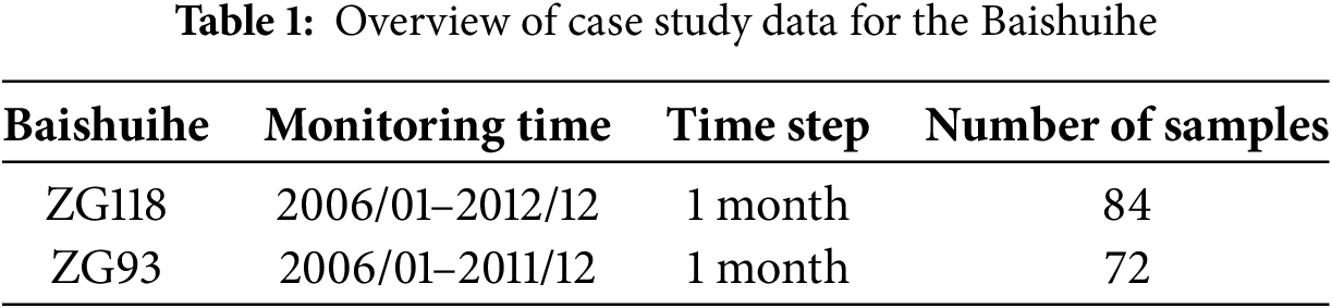
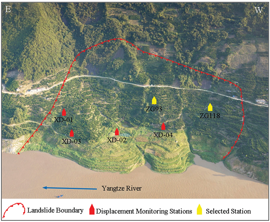
Figure 1: Layout of monitoring sites for the Baishuihe landslide [34]

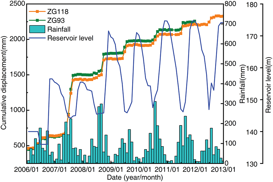
Figure 2: Changes in raw monitoring data for the Baishuihe landslide

As shown in Fig. 2, the displacement of the Baishuihe landslide increases monotonically with time and is seasonal. The obvious increase in displacement and the relative stabilization phase are from April to September and from October to April of the following year. These two time periods correspond to the time when the monthly cumulative rainfall is high and the reservoir level is low. Therefore, the change of landslide displacement has a periodicity of about one year, which is closely related to the seasonal heavy rainfall and fluctuating changes of the reservoir level.

3  Methodology

3.1 Overall Working Framework

Decomposing the cumulative displacement into multiple components facilitates more accurate analysis and prediction. In this paper, we focus on the trend displacement and the periodic displacement, which are decomposed using Empirical Mode Decomposition (EMD) [35]. The maximum number of iterations for EMD is 500. Cubic spline interpolation is used, and the number of IMFs is not restricted. The endpoint effect is handled through mirror extension. The following are the stopping criteria:

(1)   Main condition (normalized standard deviation threshold SD = 0.05): When the SD values of two adjacent iterations are both below 0.05, the IMF is determined to have converged;

(2)   Auxiliary condition (normalized standard deviation threshold SD2 = 0.5): If the single SD2 value suddenly drops below 0.5, do not stop temporarily until the main condition is met;

(3)   Global termination condition (residual energy TOL = 0.05): When the residual energy is below 5% of the original signal energy, terminate the entire EMD process.

After decomposition, the component showing a trend change is extracted as the trend displacement, and the remaining components are reconstructed into the periodic displacement. These two types of displacement components are predicted separately and then superimposed in the time series to obtain the predicted result of the cumulative displacement. Fig. 3 shows the overall working framework of this study, and the main steps involved are as follows:

•   Decompose cumulative displacement and its influencing factors, and construct a feature dataset for the baseline model using Pearson and MIC feature selection methods.

•   Use Non-dominated Sorting Genetic Algorithm-II (NSGA-II) to optimize α and β parameters in the Double Exponential Smoothing (DES) method for trend displacement prediction.

•   Design a bidirectional local attention mechanism based on historical periodic displacement calculation, and apply it to the model simultaneously with the global attention mechanism.

•   Construct a BiLSTM-RBF fusion model using the hidden state of BiLSTM.

•   Introduce the improved width of the PI as a penalty term in the loss function.

•   Conduct model evaluation, comparison, and analysis.

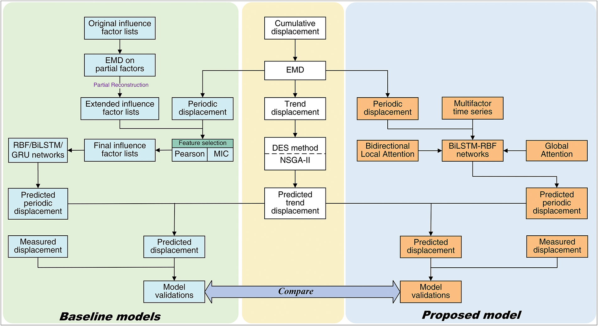
Figure 3: Overall working framework diagram

3.2 Data Preprocessing

(1)   Baseline model’s data processing

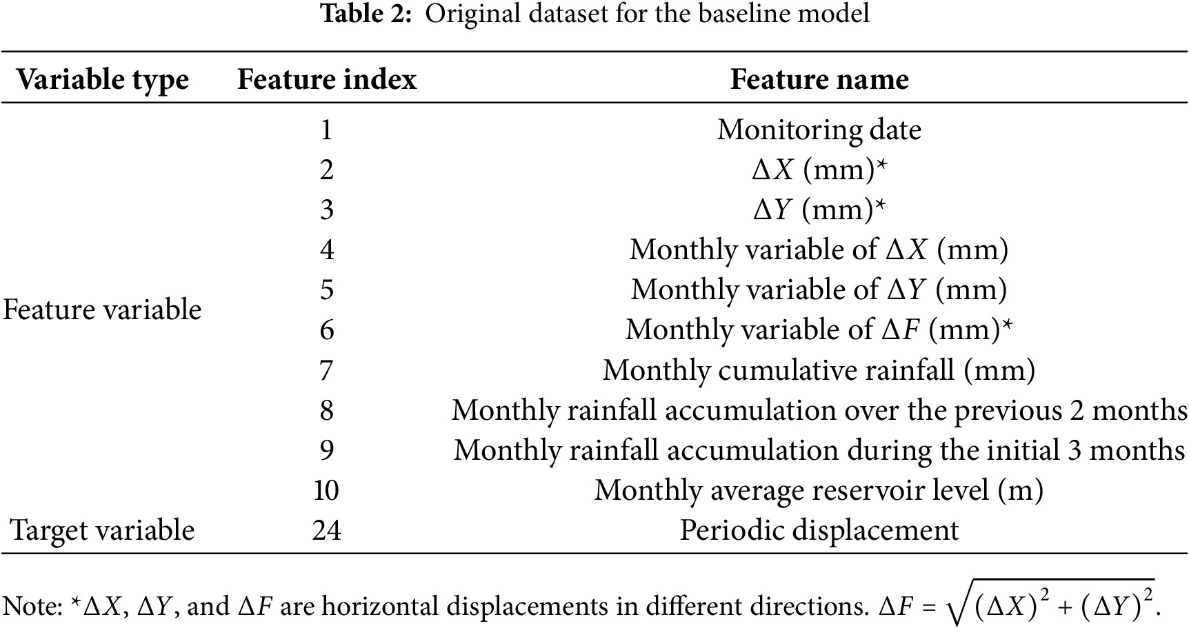
Because landslide monitoring data are time-dependent, the monitoring time is added to the data set in a specific format, e.g., January 2006 as: 200601, December 2012: 201212. The related variables with displacement, rainfall, etc., are counted to obtain the original data set for the baseline model (see Table 2). In addition, since the influencing factors (e.g., rainfall, reservoir level, etc.) also belong to seasonal external dynamics, their fluctuating changes may all have different degrees of influence on the periodic displacement. Therefore, this paper also uses EMD to decompose and partially reconstruct the monthly mean reservoir water level and monthly cumulative rainfall to obtain the extended dataset of periodic displacement.

(2)   Data splitting

To explicitly model the temporal dependence of the landslide displacement sequence, before data splitting, the sliding-window recomposition strategy is first adopted to convert the original continuous time series into the “input-output” pairs required for supervised learning. That is, each sample takes the multi-dimensional features of the previous 2-time steps as the input and the displacement value of the next time step as the target. After recomposition, the data dimension is (number of samples, 2, number of features), which can be directly used for subsequent model training. The data splitting is as follows:

(a)   Data splitting method: Considering the time series characteristics of landslide displacement data, it is necessary to strictly follow the chronological order constraint of historical data for future prediction. Therefore, this paper adopts the standard holdout strategy [16] to split the data in chronological order. This can ensure the time coherence of the data during the model training process and avoid the false improvement of model performance caused by “data leakage”.

(b)   Data splitting ratio: Since this study decomposes the cumulative displacement into trend displacement and periodic displacement for separate prediction, and the prediction models for the two types of displacement are different, the data splitting ratio for the landslide monitoring points ZG118 and ZG93 are: Trend displacement: Training set: Test set = 70%:30%; Periodic displacement: Training set: Validation set: Test set = 80%:10%:10%.

In addition, MinMax normalization is adopted to ensure the quality and consistency of input data.

3.3 Trend Displacement Prediction Model

3.3.1 DES Method

In this paper, we choose the DES method that is adaptive to a small number of data samples, especially when the data has a trend, and can adapt to the changes in the time series data. The DES method, a time series forecasting technique, is particularly suitable for data with a trend but without seasonality. This method separately predicts level changes and trend changes using two smoothing equations. The updated formulas for the level and trend equations are shown in Eqs. (1) and (2):

Lt=αYt+(1−α)(Lt−1+Tt−1),(1)

Tt=β(Lt−Lt−1)+(1−β)Tt−1,(2)

the level component at time t is denoted as Lt, α represents the smoothing coefficient for the level, Yt corresponds to the actual observation at time t, and Tt−1 indicates the trend component from the previous period. The trend component at time t is calculated as Tt, with β being the smoothing coefficient for the trend. The forecasting formula for the test set is expressed as Eq. (3):

y^t+1=Lt+Tt,(3)

where, y^t+1 is the predicted value of the test set.

3.3.2 Solving Trend Displacement Multi-Objective Optimization Problems Based on NSGA-II

NSGA-II is a multi-objective genetic algorithm proposed by Deb et al. in 2002. In multi-objective optimization, NSGA-II does not rely on explicit weighting or weighted combinations after normalization. Instead, it achieves an “implicit balance” among multiple objectives through the Pareto dominance relationship. As shown in Fig. 4a, for any two solutions A and B, if both the RMSE and MAE of A are smaller than those of B, and the R2 of A is greater than that of B, then A strictly dominates B, and B will be eliminated by the algorithm. If A is better in some indicators (e.g., lower RMSE) but worse in other indicators (e.g., higher MAE), then A and B do not dominate each other and will be jointly retained in the Pareto front. Solutions like A and B are Pareto optimal solutions. The goal of the multi-objective optimization algorithm is to find these Pareto optimal solutions [36].

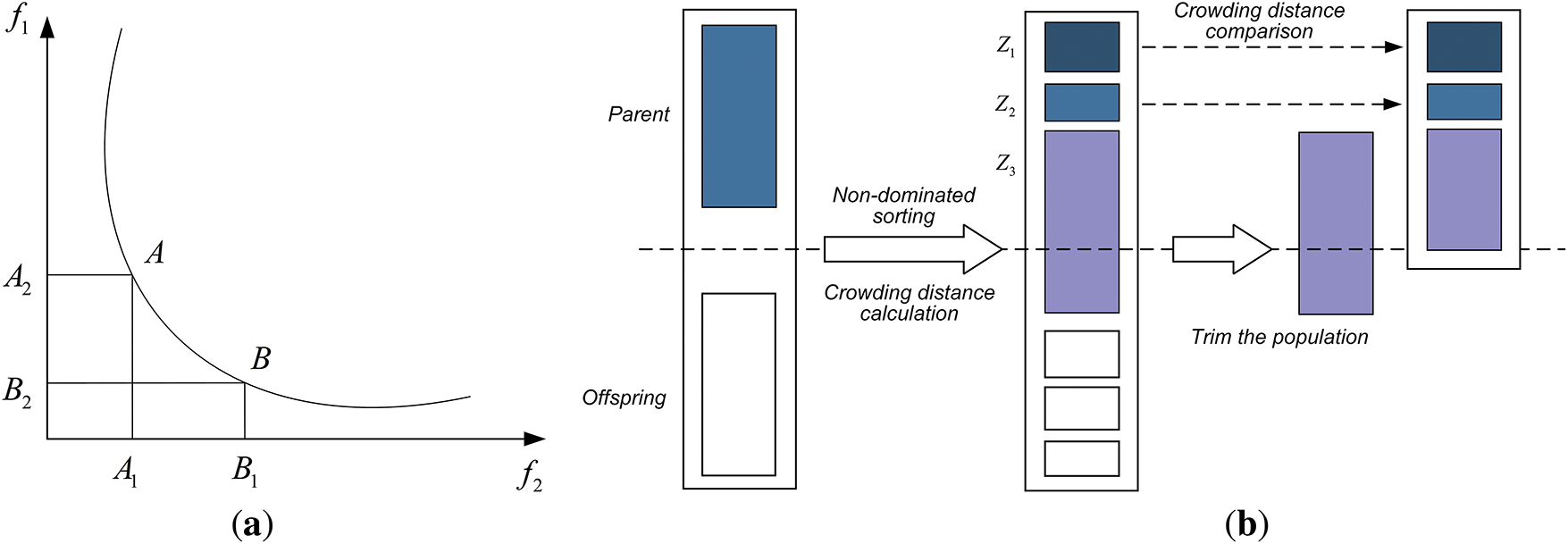
Figure 4: Main schematic diagram of NSGA-II. (a) Pareto optimal solution schematic; (b) Crowding distance comparison

As shown in Fig. 4b, when combining the generated offspring population with the parent population to form a new population, in addition to considering the non-dominated rank, the crowding distance also needs to be considered within each non-dominated layer. Each objective function will be normalized before calculating the crowding distance. The calculation of all crowding distance values is the sum of the absolute values of the differences between adjacent individuals of each individual across all objective functions. Individuals with larger crowding distances are more likely to be retained, such as Z1, Z2, and the trimmed Z3. This can prevent the individuals in the population from being overly concentrated in the objective space, ensuring that the algorithm evenly searches for the optimal solution among multiple objectives, thereby achieving a balance among multiple objectives.

Solving for the Pareto optimal solution for trend displacement. Using NSGA-II to optimize the variables α and β of the DES method. To enhance the model’s performance on new datasets, objective functions are established to minimize three evaluation metrics on the test set: f1(α,β)=RMSE, f2(α,β)=MAE, and f3(α,β)=−R2. The decision variables are the two parameters, α and β, in the DES model. The multi-objective problem is described as follows:

min{Objective1=f1(α,β)Objective2=f2(α,β)Objective3=f3(α,β)(4)

s.t.{0<α<10<β<1(5)

where, “min” means minimizing the function,

f1(α,β)=RMSE=1n∑i=1n(Yt+i−y^t+i)2=1n∑i=1n(Yt+i−(Lt+Tt))2,(6)

f2(α,β)=MAE=1n∑i=1n|Yt+i−y^t+i|=1n∑i=1n|Yt+i−(Lt+Tt)|,(7)

f3(α,β)=−R2=−(1−∑i=1n(Yt+i−y^t+i)2∑i=1n(Yt+i−Y¯)2)=−(1−∑i=1n(Yt+i−(Lt+Tt))2∑i=1n(Yt+i−Y¯)2),(8)

where Yt+i is the actual value, y^t+i is the predicted value, Y¯ is the mean of the actual values, and n is the sample size, all of which belong to the test set. The hyperparameter settings for NSGA-II are shown in Table 3.

3.4 Periodic Displacement Prediction Model

The periodic displacement prediction employs a BiLSTM-RBF fusion model enhanced by a global-local hybrid attention mechanism. Specifically, the rate of change in historical periodic landslide displacement is utilized as weights for the bidirectional local attention mechanism. Additionally, the width of the PI serves as a penalty term in the loss function.

3.4.1 Baseline Models for Periodic Displacement Prediction

By manually selecting features for three baseline models (RBF neural network, BiLSTM neural network, GRU neural network), a feature dataset for periodic displacement is constructed to prepare for the model validation of the proposed network, which does not require manual feature selection.

(1)   Feature selection methods

In order to enhance the baseline model’s prediction accuracy, we evaluated the linear and dependency relationships between influencing factors and periodic displacements in the extended dataset using the MIC and Pearson correlation coefficient [37]. As the final dataset for periodic displacements, factors with Pearson’s correlation coefficient absolute values and MIC values of at least 0.12 and 0.4 were chosen.

(2)   BiLSTM/GRU/RBF network architecture

BiLSTM/GRU neural network. BiLSTM networks, which are generated from enhancements to LSTM networks. In BiLSTM, the LSTM network is constructed as two oppositely oriented LSTM layers (Fig. 5a), which deal with the forward and reverse directions of the sequence data. LSTM is a model for optimizing Recurrent Neural Networks (RNN) [38], with a total of three computational mechanisms, namely, forgetting gates, input gates, and output gates (Fig. 5b). Each LSTM recurrent unit has an external state of the previous moment and the current moment’s input as the unit input. The internal structure of GRU is more concise than LSTM (Fig. 5c). It consists of an update gate that controls the retention of old information and the introduction of new information, and a reset gate that determines how much of the old information has been forgotten (Fig. 5d).

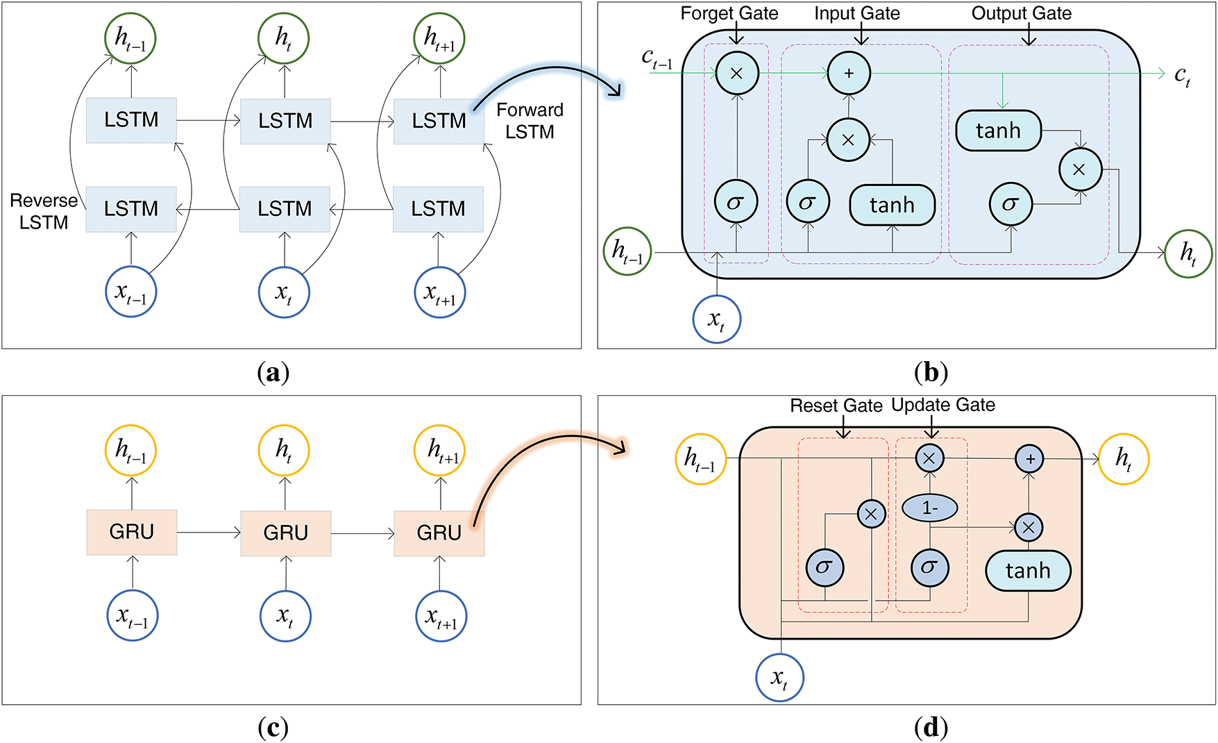
Figure 5: (a) BiLSTM neural network structure; (b) LSTM recurrent unit internal structure; (c) GRU neural network structure; (d) GRU recurrent unit internal structure

RBF neural network. The RBF neural network is a 3-layer feed-forward network with a single hidden layer and its action function is a Gaussian basis function [39]. The j-th neuron of the hidden layer is calculated in the following manner:

hj=exp⁡(−‖x−cj‖22bj2),j=1,2,…(9)

where, cj=[cj1,…,cji] and b=[b1,…,bi]T represent the center vector and the width vector of the j-th hidden layer neuron of the RBF network. The output of the RBF neural network is given by Eq. (10).

yj(t)=ω1h1+ω2h2+…+ωjhj(10)

3.4.2 BiLSTM-RBF-Attention for Periodic Displacement Prediction

(1)   Attention mechanism

Global Attention Mechanism. The global attention technique is implemented by using the popular Keras core layer (Dense). The specific steps include: input transformation, weight calculation, normalization, and application of weights. The Dense layer takes all the transformed hidden states of BiLSTM as input, calculates a raw attention score for each time step, and then converts it into normalized attention weights through the softmax function. This approach dynamically generates independent attention weights Ghwi for the hidden states at each time step by attending to the entire input sequence data.

Local Attention Mechanism. As shown in the shaded part of Fig. 6a,b, the cumulative displacement and periodic displacement of monitoring stations ZG118 and ZG93 synchronously show an upward trend, and the change is obvious. While the cumulative displacement maintains a relatively stable stage, the periodic displacement shows a decreasing trend. From this analysis, the short-term rapid increase of landslide cumulative displacement primarily originates from the increase in periodic displacement, so we must draw the model’s attention to the increasing trend while predicting the periodic displacement. As per the principle of change, this paper proposes a two-way local attention mechanism applied to BiLSTM, designing local attention weights for the forward and reverse sequences of the periodic displacement.

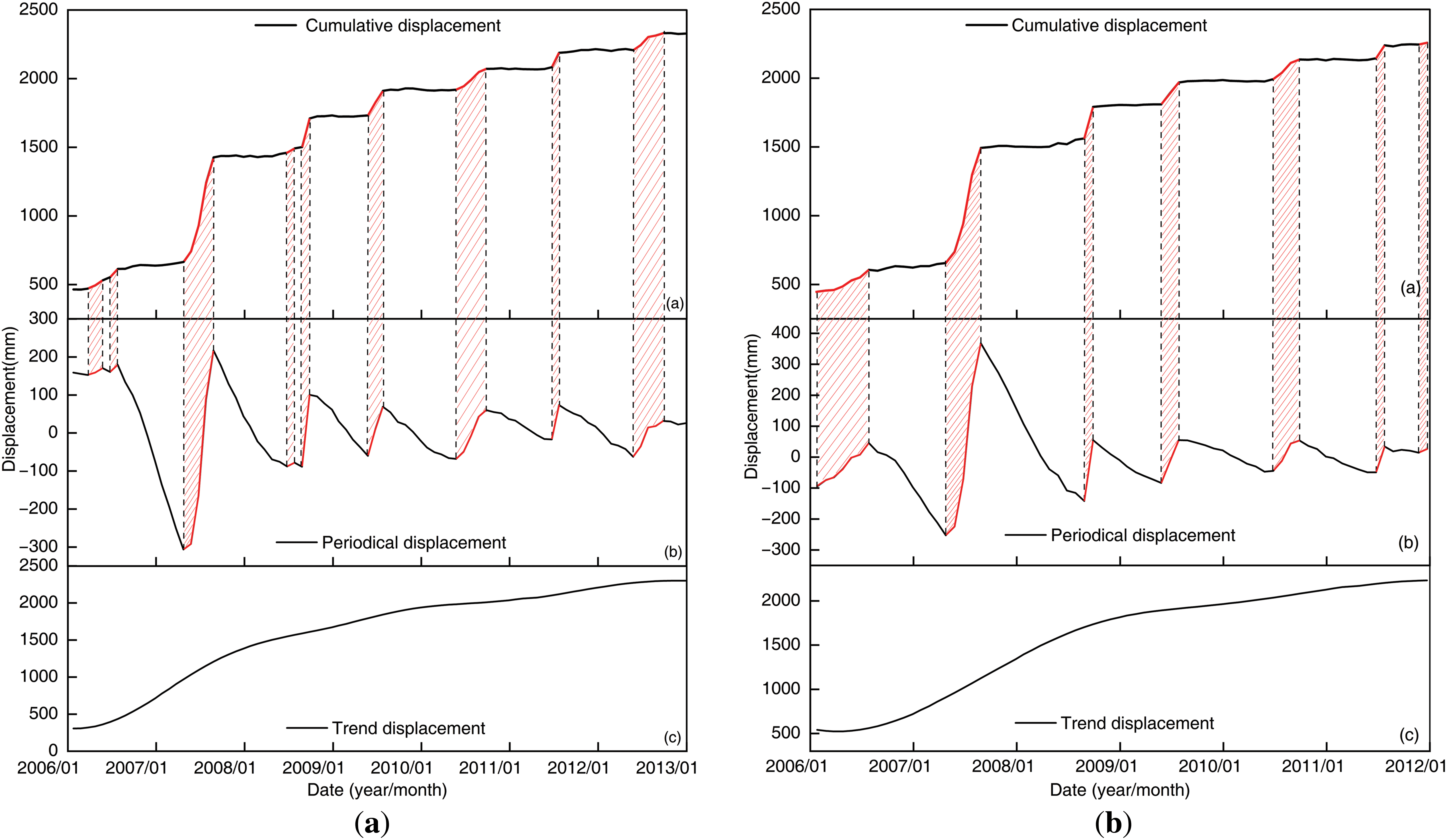
Figure 6: Cumulative displacement decomposition diagram. (a) ZG118; (b) ZG93

(a) Window size for the local attention mechanism

The window size of the local attention mechanism is fixed to 2-time steps (forward sequence: focus only on the current month displacement and the preceding month displacement in the forward periodic displacement sequence; reverse sequence: focus only on the current month displacement and the next month displacement in the reverse periodic displacement sequence), and the window sliding step size is one month.

(b) Weights of the local attention mechanism

Since the periodic displacement shows a notable increasing trend in the short term and to prevent data leakage, the historical rate of change of the periodic displacement is adopted as the local attention weights. To convert the final attention scores to the range between 0 and 1 and focus the local attention mechanism on periodic displacement sequences with an increasing trend, ending with the application of the sigmoid function. The attention weights for the forward and reverse periodic displacement sequences are denoted as wFi and wRi, as shown in Eqs. (11) and (12):

wFi={0,i=0sigmoid((PFi−PF(i−1))/1),i≠0(i=0,1,2,…,n)(11)

wRi={0,i=n−1sigmoid(−(PR(i+1)−PRi)/1),i≠n−1(i=0,1,2,…,n)(12)

where, PFi and PRi represent the forward and reverse periodic displacements at the time step i.

Apply the forward attention weights to the hidden states of the forward LSTM layer and the reverse attention weights to the hidden states of the reverse LSTM layer (Eqs. (13) and (14)). Then, concatenate the weighted hidden states of the forward and reverse directions at corresponding time steps to obtain the hidden states of the BiLSTM after the application of bidirectional local attention weights, as shown in Eq. (15), Fig. 7:

hwFi=hFi⋅wFi(13)

hwRi=hRi⋅wRi(14)

Lhwi=hwFi⊕hwR0(15)

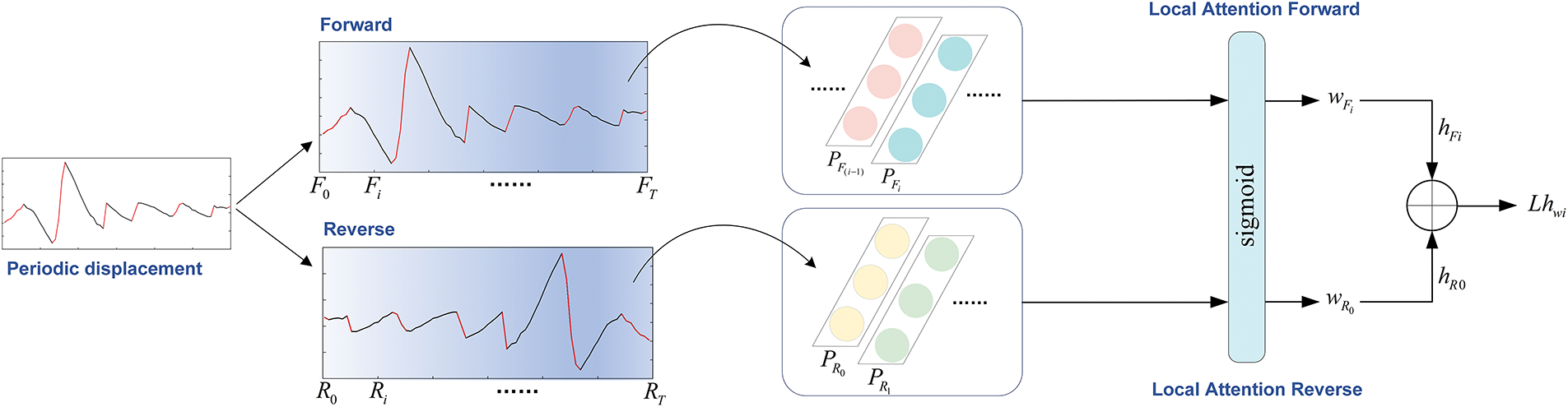
Figure 7: Schematic diagram of bidirectional local attention mechanism

In summary, the global-local hybrid attention mechanism is simultaneously applied to the weighted concatenated hidden states following the BiLSTM hidden states, as shown in Eq. (16):

bhi=Ghwi+Lhwi(16)

(2)   Loss function

The PI is an important concept in statistics, which provides a range to estimate the possible values of future observations. To construct a PI, the mean of the predicted values is used as the center of the interval, and the standard deviation of the residuals is considered to reflect the variability of the data. In the study, the PI is built on the foundation of the normal distribution, with a confidence level set at 95%. The mathematical formula for the PI is Eq. (17):

PI=y^±Z1−α⋅Spred,(17)

where, y^ is the model’s predicted value, Z1−α is the critical value of the normal distribution, and Spred is the standard error of the prediction. From Eq. (17), the width of the PI WPI′ is derived as:

WPI′=(y^+Z1−α⋅Spred)−(y^−Z1−α⋅Spred)=2⋅Z1−α⋅Spred(18)

Construct a loss function that uses the width of the PI as a penalty term, to penalize the width when the model’s predicted value deviates from the observed value. Therefore, this paper replaces the model’s predicted standard error Spred with the batch Mean Absolute Error (MAEbatch), and the improved width of the PI is:

WPI=2⋅Z1−α⋅MAEbatch(19)

The final loss function is as in Eq. (20):

Loss=MSE+λ⋅WPI,(20)

where, λ is a hyperparameter that balances the weights of the MSE and WPI.

(3)   Periodic displacement prediction based on BiLSTM-RBF-Attention

Fig. 8 shows the structure of the proposed model, which directly takes the original time series data as its input (ZG118: reservoir level and historical displacement; ZG93: monthly cumulative rainfall, reservoir level, and historical displacement). All of the weighted hidden states bhi of BiLSTM are used as inputs to the RBF neural network. The “expand_dims” operation in TensorFlow is used to add the necessary dimensions to the input of the RBF to integrate the weighted hidden states of the BiLSTM. The specific process includes: First, obtain the weighted hidden states of the BiLSTM as the input tensor “inputs”, whose shape is (batch_size, time_steps, 2LSTM_units). Second, add a single dimension after the feature dimension through “tf.expand_dims (inputs, -1)” to convert it to “(batch_size, time_steps, 2LSTM_units, 1)”. Then, broadcast the RBF center tensor “centers” with the shape of “(2LSTM_units, RBF_neurons)” to match the shape of the input tensor, broadcasting it to (1, 1, 2LSTM_units, RBF_neurons). After broadcasting, the shapes of the two are compatible, enabling element-wise difference calculation. By using the method of taking the output of BiLSTM as the input of RBF, the effective integration of the two models is achieved.

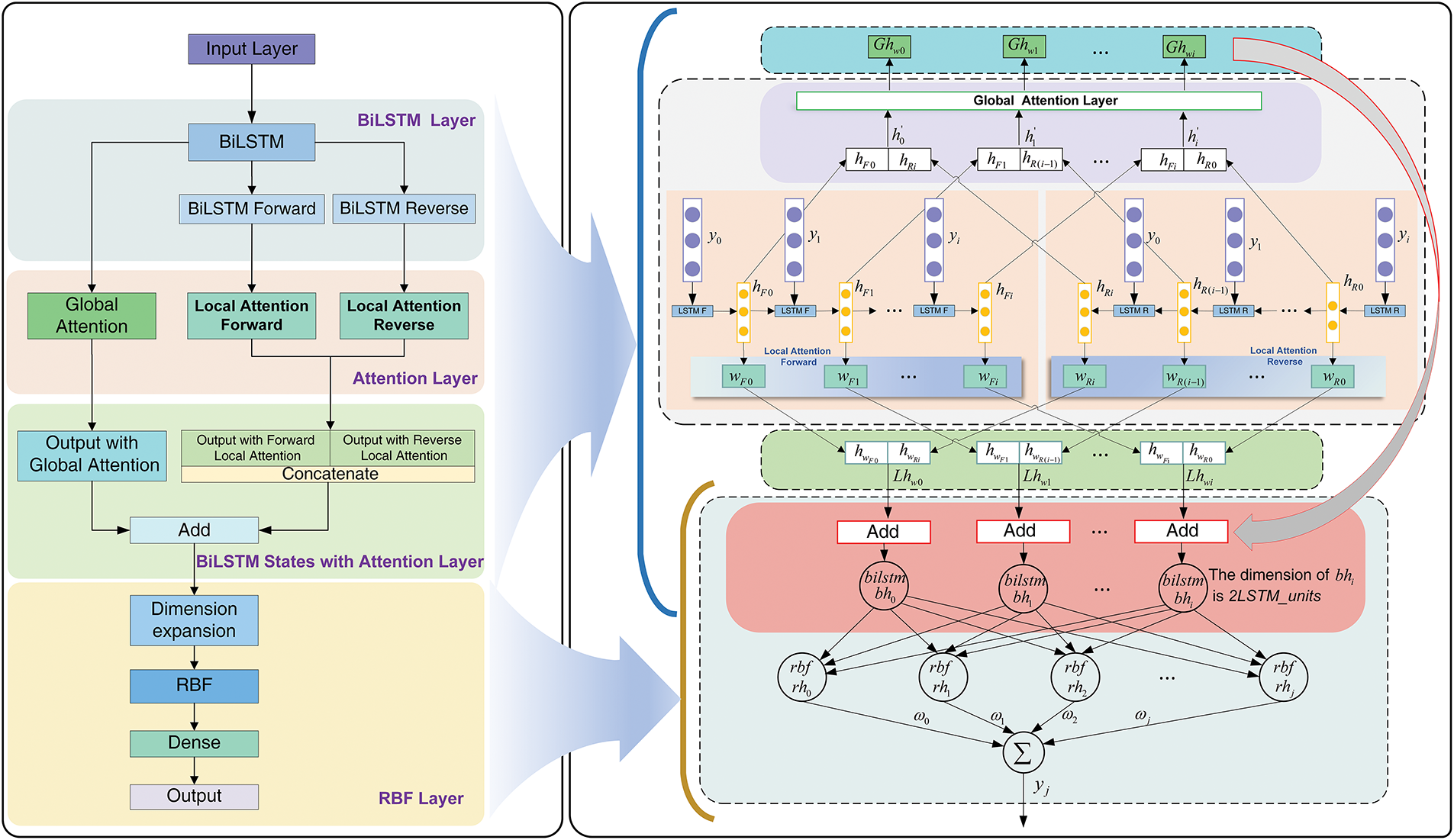
Figure 8: Structure of BiLSTM-RBF-Attention model

Model parameter settings: the model was trained in CPU mode on Intel (R) Iris (R) Xe Graphics integrated graphics card, implemented using TensorFlow 2.15.0 and keras framework, and the programming language was Python (Python 3.9). After experimental testing, the training parameters of BiLSTM-RBF-Attention were finally set as follows: epochs = 200, learning rate (Adam optimizer) = 0.001, batch = 2, LSTM_units (ZG118) = 64, LSTM_units (ZG93) = 32, RBF_units (ZG118) = 96, RBF_units (ZG93) = 64, and the loss function penalty coefficients λ are 1×10−5 and 1×10−4. Setting independent random seeds for the data characteristics of different landslide monitoring points, at ZG118: (NumPy: 0, TensorFlow: 1); at ZG93: (NumPy: 6, TensorFlow: 8).

3.5 Evaluation Metrics

In this paper, the evaluation metrics shown in Table 4 are selected to compare and analyze the landslide displacement prediction models objectively. Model predictive fidelity exhibits an inverse proportionality to residual error magnitudes, as quantified by diminishing root mean square error (RMSE) and mean absolute error (MAE) values. The coefficient of determination (R²), bounded between 0 and 1, serves as a critical diagnostic metric, with values closer to 1 signifying enhanced congruence between simulated surface deformation and observational datasets.

4  Results

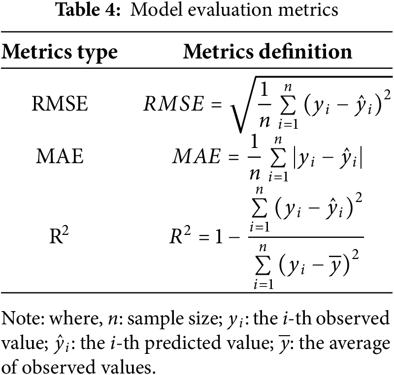
Fig. 6 illustrates the cumulative displacement decomposition results of the Baishuihe landslide monitoring points ZG118 and ZG93. After EMD is completed, the mean values of the residuals of ZG118 and ZG93 are 6.16×10−15 and −1.92×10−14 respectively, and the slopes of the linear trends are −3.88×10−16 and −8.20×10−17, respectively. Moreover, the histograms show a symmetric distribution (Fig. 9a,b), which meets the theoretical requirements of EMD for zero-mean and trend-free residuals, verifying the completeness of the decomposition.

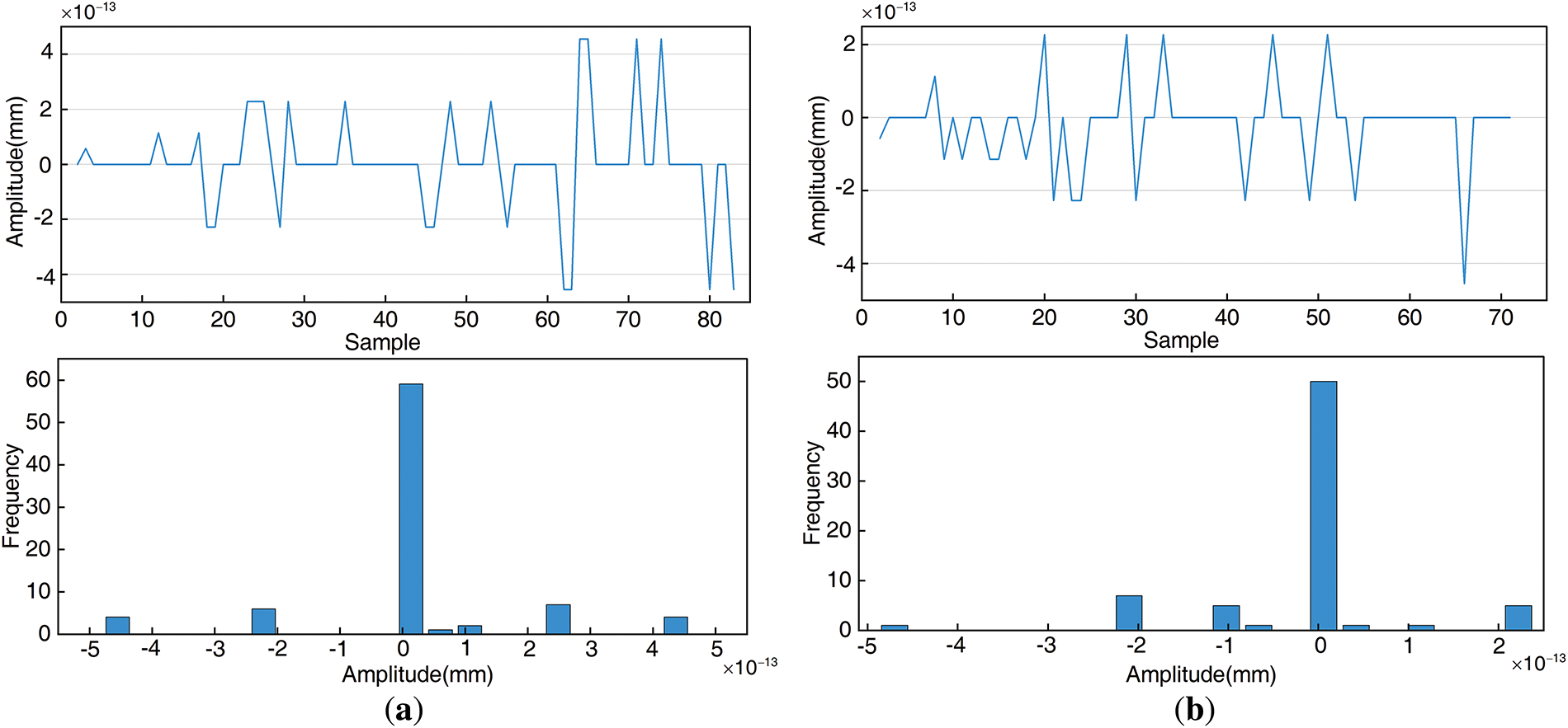
Figure 9: Residual graph and residual distribution graph based on EMD. (a) ZG118; (b) ZG93

In Fig. 6, the shaded area represents the change rule of the cumulative displacement, which is characterized by a distinct upward trend as the periodic displacement increases. This is equivalent to the calculation principle of Eqs. (11) and (12).

4.1 Trend Displacement Prediction Results

From the obtained Pareto front (Fig. 10a,b), the most suitable Pareto solution (highlighted in red) was selected by comprehensively evaluating the performance of RMSE, MAE, and R² on both the training and test sets. The Pareto decision variables for ZG118 and ZG93 are (α: 0.96637, β: 0.00035) and (α: 0.86971, β: 0.00052), respectively.

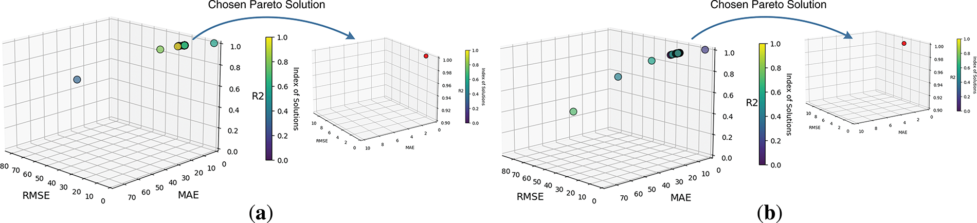
Figure 10: Pareto front of DES. (a) ZG118; (b) ZG93

Fig. 11a,b displays the trend displacement prediction results for the Baishuihe landslide at monitoring locations ZG118 and ZG93. The Pareto optimal solution produced RMSE, MAE, and R2 values of 0.35, 0.29 and 0.99 mm for ZG118; for ZG93, the corresponding metrics were 1.02, 0.93 and 0.99 mm.

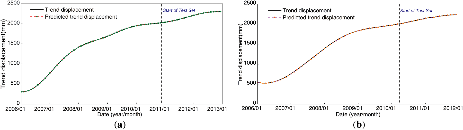
Figure 11: Results of the trend displacement prediction. (a) ZG118; (b) ZG93

4.2 Periodic Displacement Prediction Results

4.2.1 Feature Selection for Baseline Models

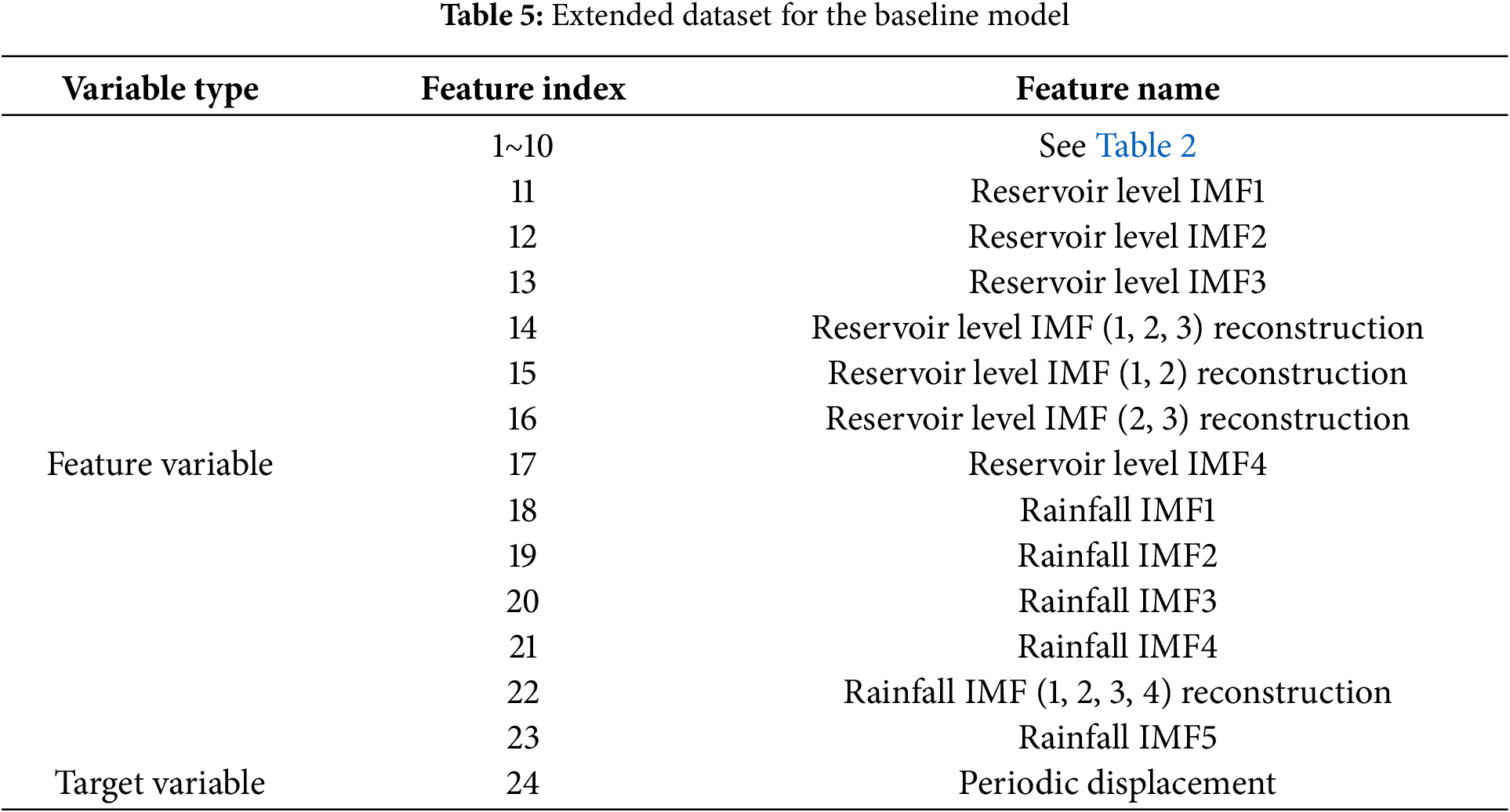
Fig. 12a,b shows the decomposition results of the reservoir level and monthly cumulative rainfall. The extended dataset for the baseline model is obtained from these results (see Table 5).

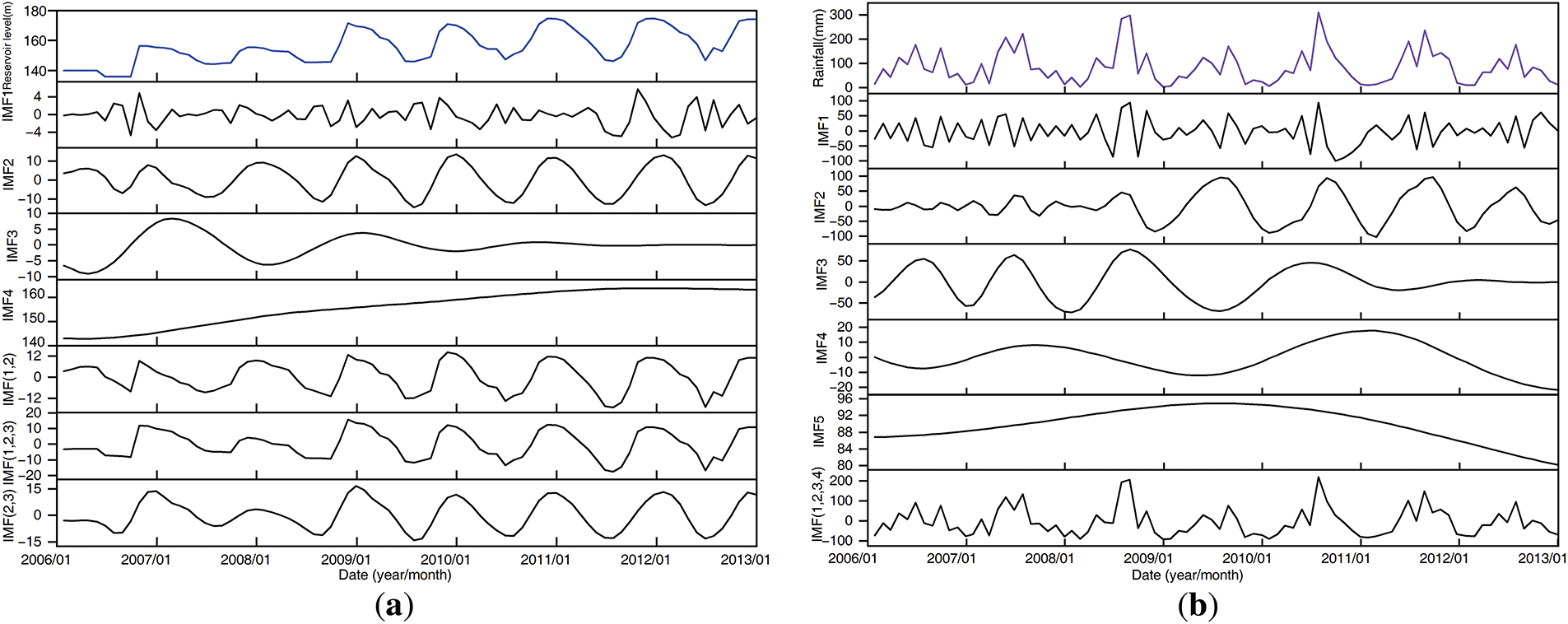
Figure 12: Decomposition and partial reconstruction results of features. (a) Reservoir level; (b) monthly cumulative rainfall

The feature selection processes using Pearson and MIC are presented in Figs. 13a,b and 14a,b for the extended datasets for monitoring points ZG118 and ZG93. In summary, the final dataset index for monitoring point ZG118 were determined as Pearson-selected features: 9, 15, 12, 6, 18, 13 and MIC-selected features: 3, 2, 23, 17, 1, 10, 13. while for ZG93, the corresponding index were Pearson: 5, 4, 6, 2, 3, 9, 21, 22, 7, 18, 20, 13 and MIC: 17, 13. Consequently, the surface displacement and deformation of the ZG118/ZG93 landslide monitoring site are influenced to varying degrees by the fluctuation components of the characterisation variables. For the ZG118/ZG93, feature factor 13 (Reservoir level IMF3) is chosen in both feature selection techniques, demonstrating both a complex nonlinear connection and a high linear correlation with the periodic displacement. It has more stability as a baseline model feature factor.

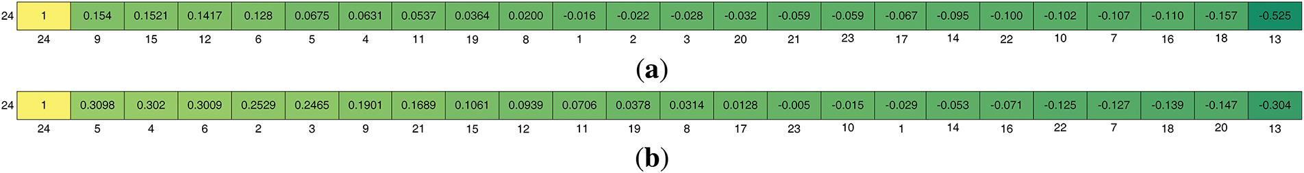
Figure 13: Feature selection heatmap of Pearson. (a) ZG118; (b) ZG93

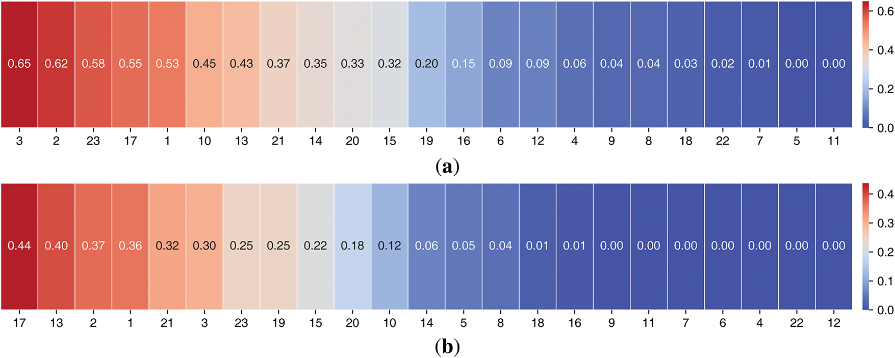
Figure 14: Feature selection heatmap of MIC. (a) ZG118; (b) ZG93

4.2.2 Model Evaluation

The results of the periodic displacement prediction for the ZG118 and ZG93 (Fig. 15a,b) demonstrate that the BiLSTM-RBF model proposed in this study, which integrates a global-local hybrid attention mechanism, significantly outperforms baseline models requiring manual feature selection. As shown in Fig. 16a,b, the BiLSTM-RBF model achieved the lowest RMSE (ZG118: 10.45 mm; ZG93: 10.16 mm) and MAE (ZG118: 7.46 mm; ZG93: 9.15 mm) values and the highest R² (ZG118: 0.91; ZG93: 0.90) scores at both monitoring points (the “None” option in feature selection methods indicates the direct use of monthly cumulative rainfall, reservoir water levels, and historical displacement as inputs). Notably, after feature selection based on the Pearson and MIC, the RBF neural network exhibited superior predictive performance compared to predictions using raw data inputs.

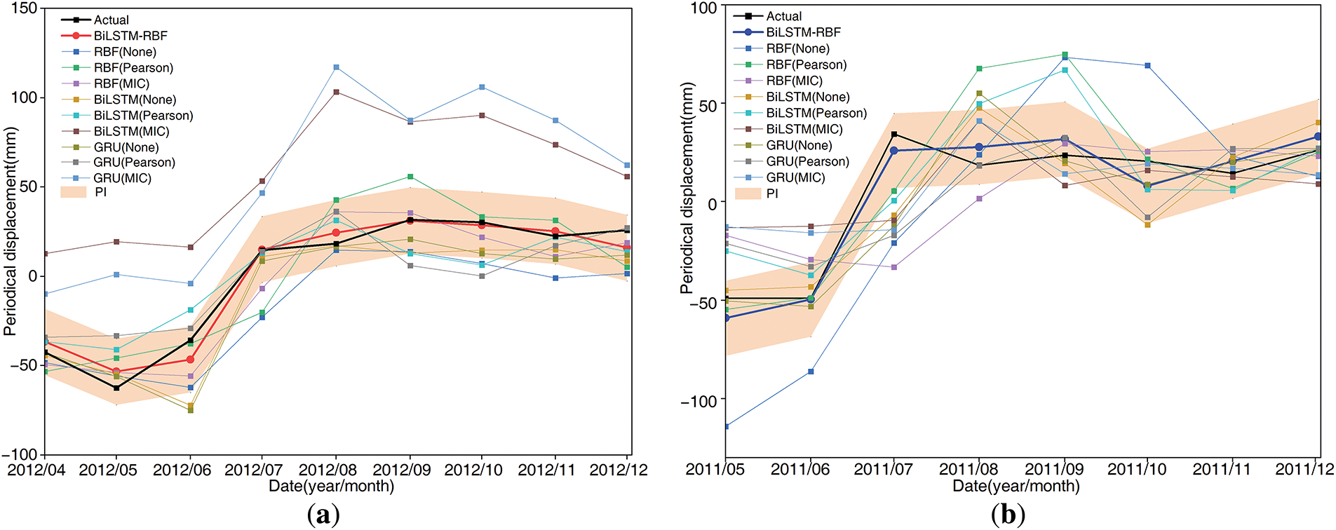
Figure 15: Results of the periodic displacement prediction. (a) ZG118; (b) ZG93

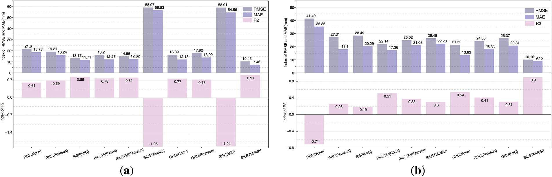
Figure 16: Model validation for periodic displacement prediction. (a) ZG118; (b) ZG93

Among baseline models, the BiLSTM and RBF models showed better prediction accuracy for ZG118 than for ZG93 after feature decomposition. Furthermore, analysis of the ZG118 prediction results revealed that although RBF-MIC and BiLSTM-Pearson demonstrated higher accuracy, their evaluation metrics remained inferior to those of the proposed model. For ZG93 with a smaller sample size, baseline models exhibited suboptimal predictive performance even after feature selection, while the proposed model consistently achieved the best and most stable results. Moreover, the PIs of ZG118 and ZG93 both meet the expected coverage requirements for the actual data.

As shown in Fig. 17a,b, at the ZG118 and ZG93 monitoring points, compared with the RBF, BiLSTM, and GRU series models, the median error of BiLSTM-RBF is significantly lower and the dispersion is smaller (in the box-plot, the box of BiLSTM-RBF is the shortest and the whiskers are the narrowest), which proves that its performance advantage is not due to random fluctuations but a stable effect brought by the model structure (hybrid attention, bidirectional time-series modeling, and RBF fusion).

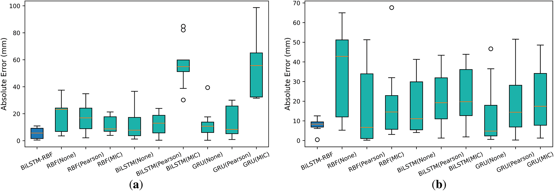
Figure 17: Box plot of the Wilcoxon test. (a) ZG118; (b) ZG93

4.2.3 Ablation Experiment

In order to verify the effectiveness and role of the introduced components, as well as the impact of different activation functions on local attention, ablation experiments were conducted on the Baishuihe ZG118 and ZG93 datasets. To ensure that the comparison between ablation experiments is only caused by the difference of the target variable, and all experiments use the same random seed as the main model. In Table 6, “✓” and “❌” respectively indicate whether the component is enabled, and each row gives the corresponding indicator.

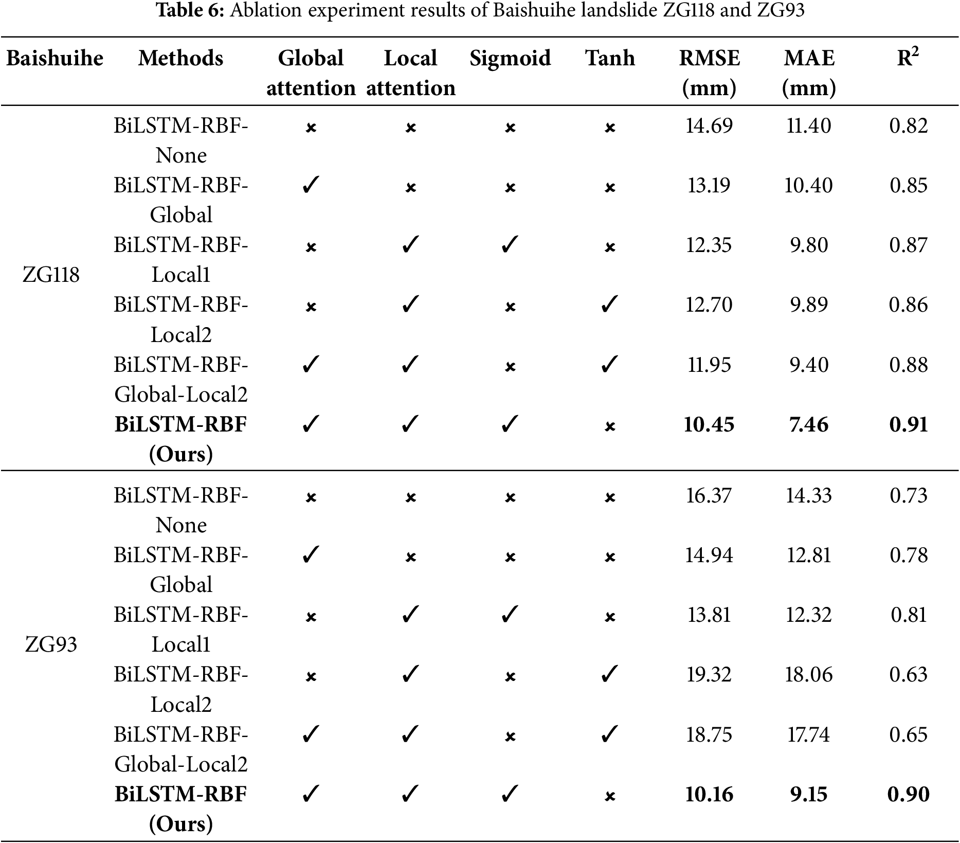
The results in Table 6 indicate that:

(1)   Whether attention is introduced or not, the fusion of BiLSTM and RBF is superior to single BiLSTM or RBF, proving the effectiveness of this structure itself.

(2)   In ZG118, after introducing global and local attention separately or jointly, compared with BiLSTM-RBF-None without attention, RMSE decreases by 10.2%–28.9%, MAE decreases by 8.8%–34.6%, and R² increases by 3.7%–11.0%, verifying the effectiveness and complementarity of the two types of attention. In addition, by comparing the two groups of models, BiLSTM-RBF-Local1 and BiLSTM-RBF-Local2, and BiLSTM-RBF-Global-Local2 and BiLSTM-RBF (Ours), it is verified that using sigmoid in local attention is more stable than tanh.

(3)   In ZG93, both global attention (BiLSTM-RBF-Global) and local attention using sigmoid (BiLSTM-RB-Local1) are superior to BiLSTM-RBF-None without attention, verifying the effectiveness of each component again. In addition, when the local attention uses the tanh activation function, the R² values of BiLSTM-RBF-Local2 and BiLSTM-RBF-Global-Local2 are 0.63 and 0.69 respectively, which are not only lower than that of the method proposed in this paper (0.90), but even lower than that of BiLSTM-RBF-None without attention (0.73), further proving the advantages of sigmoid in terms of stability and performance.

In summary, it shows that the global attention mechanism effectively captures the long-term dependency relationship of landslide displacement, while the bidirectional local attention mechanism accurately extracts short-term local features.

4.3 Cumulative Displacement Prediction Results

Fig. 18a,b shows the cumulative displacement prediction results corresponding to the test set of trend and periodic displacements for the two landslide monitoring sites, and the evaluation metrics are shown in Fig. 19a,b, where the experimental results show that the overall prediction accuracies of the BiLSTM-RBF model are all better than the baseline model.

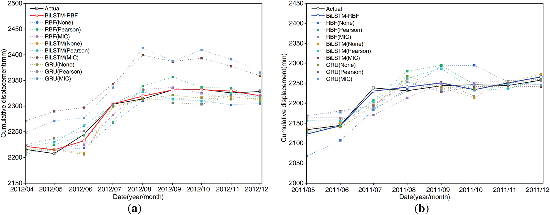
Figure 18: Results of the cumulative displacement prediction. (a) ZG118; (b) ZG93

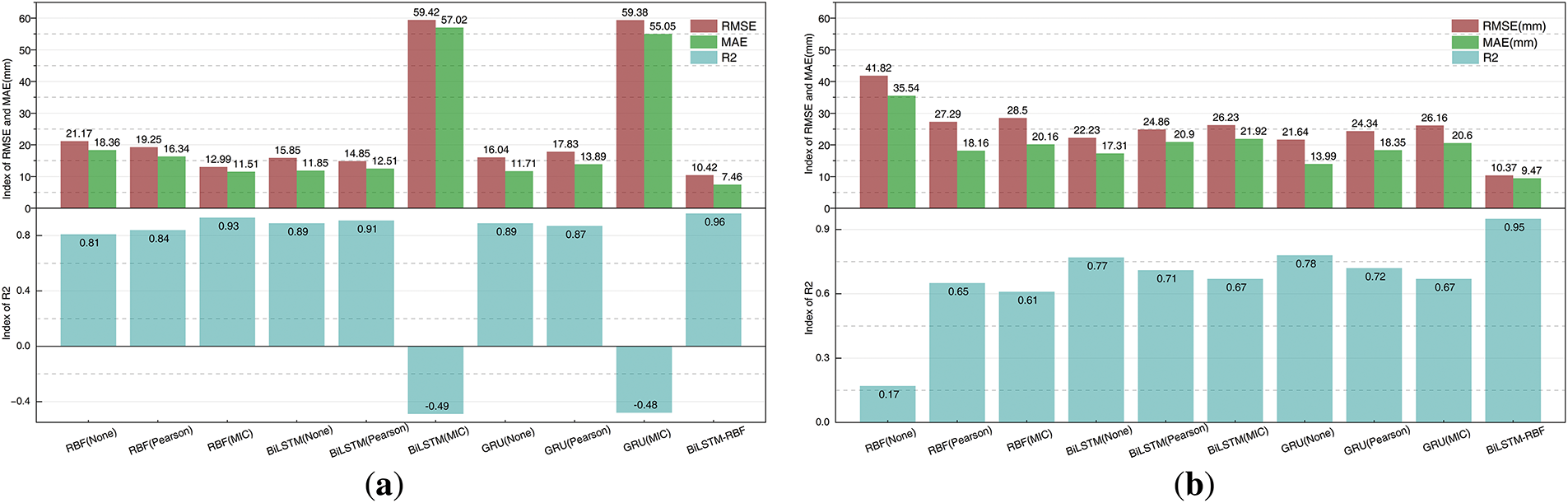
Figure 19: Model validation for cumulative displacement prediction. (a) ZG118; (b) ZG93

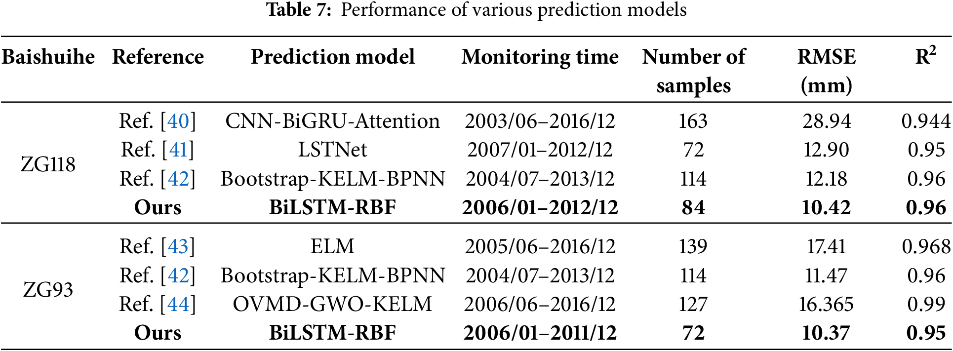
As shown in Table 7, the model in this paper is compared with other models with larger sample sizes under the most restricted condition with the smallest sample size. It shows that the RMSE of this paper’s model is the lowest in both monitoring points ZG118 and ZG93. The BiLSTM-RBF prediction model is confirmed to be superior by the performance comparison of the aforementioned models. The improved performance of this paper’s proposed model mostly depends on:

(1)   The historical periodic displacement data are used to construct a bidirectional local attention mechanism for BiLSTM, which enhances the model’s bidirectional adaptive feature extraction from the original input.

(2)   The global attention acts on the combined hidden state of BiLSTM, and the local attention acts on the hidden state of the forward and reverse layers of BiLSTM, and the hybrid global-local attention mechanism enhances the model’s feature extraction capability.

(3)   By fully utilizing the hidden states of BiLSTM to drive RBF neural network for nonlinear feature mapping, the model can extract the features of the weighted hidden state more efficiently, thus capturing the key features of the data at multiple levels under the condition of limited data, and further improving the performance of the model.

5  Discussions

BiLSTM constitutes an efficient deep learning model by combining forward and reverse information. However, the traditional global attention mechanism is directly applied to its concatenated hidden states, which makes the process of successfully extracting bidirectional characteristics from sequence data challenging. For this reason, this study proposes a bi-directional local attention mechanism based on historical displacement data to enhance bi-directional feature recognition and trend-capturing capabilities. Additionally, an RBF neural network is included to improve the model’s effectiveness in recognizing data patterns.

(1)   When optimizing the smoothing coefficients of the DES using NSGA-II, constraining the range of individual mutation is crucial to obtain the optimal solution, which can dynamically adjust the smoothing coefficients in accordance with the number of samples, and the optimized coefficients are better than the current widely used parameters of the DES [34]. In periodic displacement prediction, although batch-level optimization is achieved by using the width of the PI as a penalty term in the loss function, independent optimization for each individual time step has not been realized. Additionally, the penalty coefficient λ needs to be adjusted according to the change in the sample size. However, the impact of the λ value on the model performance is nonlinear, which makes it a challenge to balance the prediction accuracy and the coverage rate of the prediction interval. These limitations will be the focus of future improvements to the loss function structure.

(2)   From Fig. 16, the improvement effect of feature decomposition on the neural network relies upon the combination of the model and the feature selection method. The degree of improvement effect is different in ZG118 and ZG93 monitoring points, and even performance degradation occurs in BiLSTM-MIC and GRU-MIC. However, in the RBF-MIC and BiLSTM-Pearson at monitoring site ZG118, and the RBF-Pearson and RBF-MIC baseline models at monitoring site ZG93, the RMSE, MAE, and R2 were all better than those of using the raw temporal input data (monthly cumulative rainfall, reservoir level, and historical periodic displacement) directly. Therefore, it is crucial to perform feature factor decomposition before manual feature selection, but it is necessary to choose the appropriate feature selection method and neural network model.

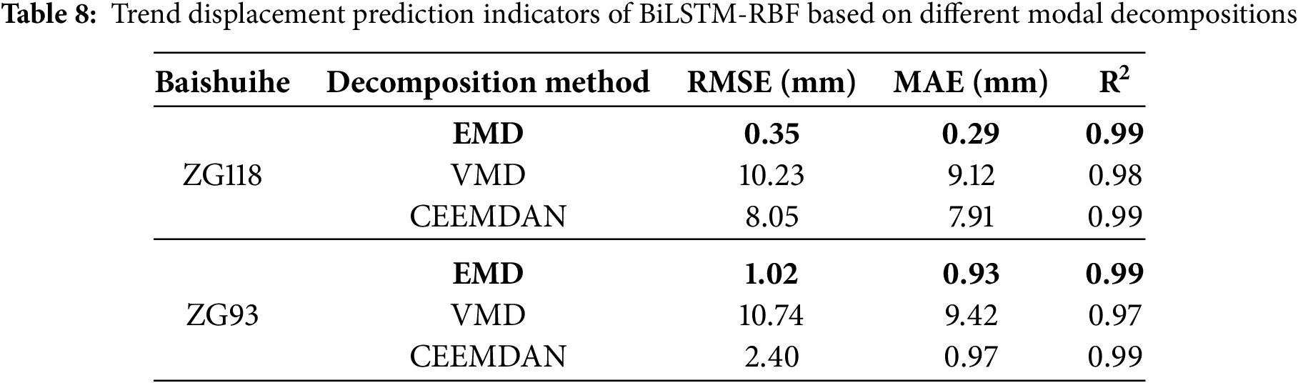
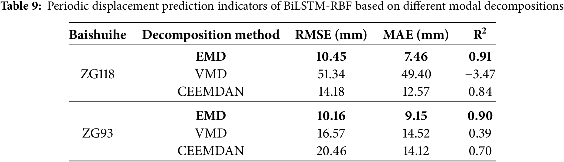
(3)   To further verify the robustness of the feature decomposition method, this study compared the impacts of EMD, Variational Mode Decomposition (VMD), and Complete Ensemble Empirical Mode Decomposition with Adaptive Noise (CEEMDAN) on the model prediction performance. For each decomposition method, the same processing procedure as that of EMD was adopted: the component showing a trend change was extracted as the trend displacement, and the remaining components were reconstructed into the periodic displacement. Meanwhile, using the same model parameters as those based on EMD decomposition, the periodic displacement and trend displacement of the monitoring points ZG118 and ZG93 of Baishuihe landslide were predicted and analyzed, respectively. By comparing the prediction results (see Tables 8 and 9), it can be seen that the VMD performed the worst in both the prediction of trend displacement and periodic displacement, while the performance of CEEMDAN was significantly better than that of VMD. It is worth noting that under the condition of the same model parameters, the three model evaluation indicators for the prediction of trend displacement and periodic displacement based on EMD were still the best, indicating that under the model framework combined with the hybrid attention mechanism in this paper, the boundary effect of EMD can be significantly improved through data-driven feature extraction. Overall, the prediction results of the model based on EMD proposed in this paper have good robustness.

(4)   In the BiLSTM-RBF model for periodic displacement prediction of the Baishuihe landslide, when compared with the best baseline model, the RMSE, MAE, and R² of ZG118 improved by 2.72, 4.25 and 0.06 mm; In ZG93, the three metrics improved by 11.36, 4.48 and 0.36 mm. which confirmed the model’s ability to predict the displacement of landslides accurately. Table 10 compares the total running time and the number of model parameters for a single run (epochs = 200) in predicting periodic displacement. These include the BiLSTM-RBF model with raw time series data as input and the baseline model under different feature selection methods (the running time of the baseline model excludes the time needed for manual feature selection). This shows that model type, number of neurons, number of features, and number of samples all affect the model run time and number of model parameters to varying degrees. Specifically, the number of neurons has the most impact on model parameters.

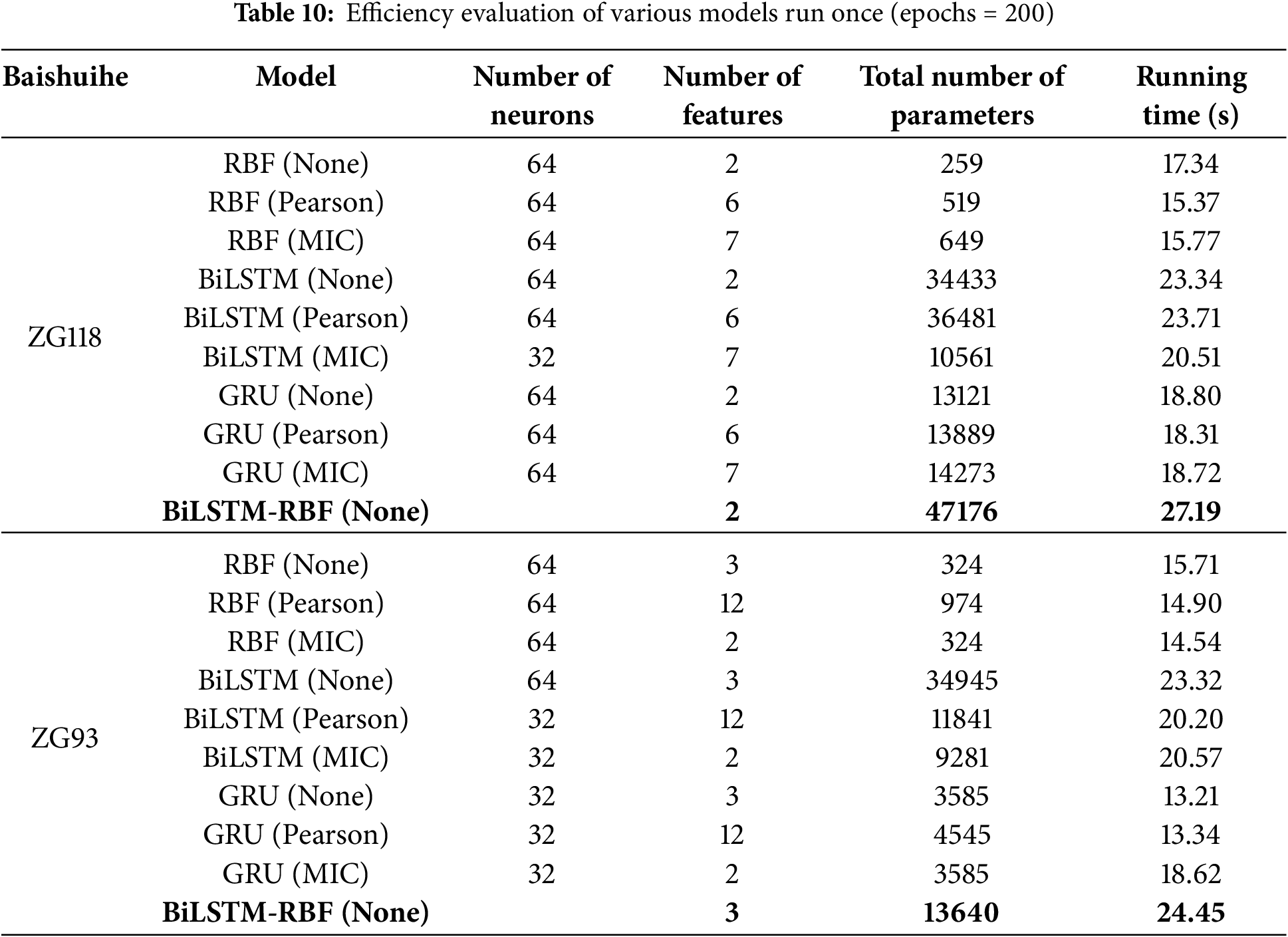
As in Fig. 20, to quantify the model efficiency, the “time consumption per parameter” (i.e., the running time divided by the number of parameters) is introduced to reflect the slope k of the linear fitting of the relationship curve between the running time and the number of parameters. A steeper slope (larger k) means that a small increase in the number of parameters will lead to a significant increase in the running time, indicating that the model is more “inefficient” in terms of computing resource utilization. A gentler slope (smaller k) indicates that parameter expansion has a small impact on the running time, resulting in higher computational efficiency. Therefore, the model run at monitoring point ZG118 showed the greatest prediction efficiency. At monitoring point ZG93, the run efficiency was second only to the baseline models BiLSTM (None) and BiLSTM (Pearson), but compared to the most efficient BiLSTM (None), the model parameters were reduced by about 2.5 times, while the run time increased by only 4.85%, indicating that the model memory footprint was significantly reduced without sacrificing real-time performance.

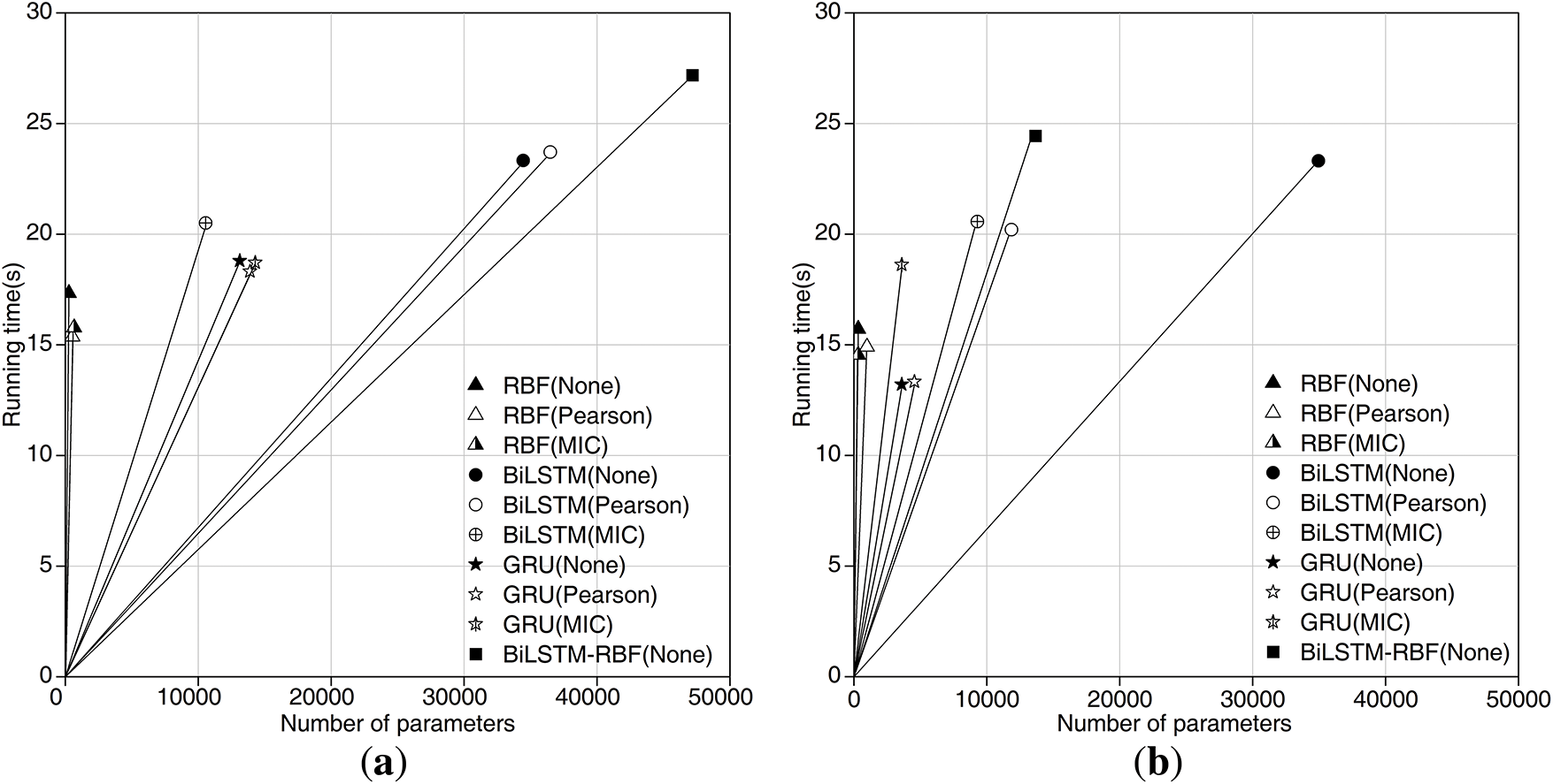
Figure 20: Visual analytics for the efficiency evaluation. (a) ZG118; (b) ZG93

(5)   In Table 7, this study verifies the effectiveness of the proposed model in overcoming data scarcity and making full use of historical data through model comparison under different sample sizes. Except for the LSTNet model in Reference [41], the number of monitoring samples used in this study (84 and 72 samples for ZG118 and ZG93, respectively) is less than that of other literature models. Especially in References [40] and [43], the sample size used in this study is almost half of theirs, while the proposed model still achieves the lowest RMSE. However, each model is trained and tested on time series of different lengths. This difference directly leads to limitations in model performance evaluation. Future research can conduct model training and comparison on a dataset with a unified time span and sampling frequency to ensure the comparability and rigor of the results.

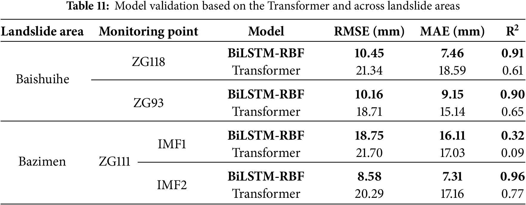
(6)   This model constructs a more efficient prediction framework. However, to further verify its adaptability and robustness in current mainstream time series prediction models and for different geological landslides, this paper selects the Bazimen landslide, which has significant differences in geological background, deformation mechanism, and inducing factors from the Baishuihe landslide, to further verify the generalization of the model and compares it with Transformer. The selected monitoring points and time period are: ZG111, 2007/01–2012/12, with 72 samples. The data preprocessing strictly follows the established process of the Baishuihe landslide. Two periodic displacement components, IMF1 and IMF2, of the Bazimen landslide are decomposed through EMD. Model parameter settings: The same model parameters for IMF1 and IMF2 are: epochs = 200, learning rate = 0.001, batch=2. The data splitting in chronological order (Training set: Validation set: Test set = 60%: 10%: 30%). Other model parameters: LSTM_units (IMF1) = 5, LSTM_units (IMF2) = 20, RBF_units (IMF1) = 20, RBF_units (IMF2) = 100. In IMF1 and IMF2, the penalty coefficients of the loss function λ are 0.1 and 0.01 respectively, the random seeds are respectively: (NumPy: 1, TensorFlow: 5) and (NumPy: 1, TensorFlow: 2). The experimental results in Table 11 show that the model proposed in this paper demonstrates the optimal performance in the displacement prediction of the Bazimen landslide across regions and when compared with the current mainstream Transformer models. This fully verifies that the BiLSTM-RBF model with a hybrid attention mechanism has good migration ability under different geological conditions.

6  Conclusion

In this study, we propose a BiLSTM-RBF model with global and bidirectional local attention mechanisms, which can directly take raw time series data as inputs and is appropriate for landslide displacement prediction with a limited sample size. By designing an interpretable attention mechanism, all hidden states of BiLSTM are fully applied to realize pattern recognition and the full extraction of landslide monitoring data features. From results of the cumulative displacement prediction for the Baishuihe landslide (Fig. 19): at monitoring point ZG118, the evaluation metrics of BiLSTM-RBF, RMSE, MAE, and R2, are all improved by 2.57, 4.05 and 0.03 mm compared with the best-performing baseline model (RBF-MIC). At monitoring point ZG93, all three metrics are improved by 11.27, 4.52 and 0.17 mm compared with the best-performing baseline model (GRU-None). Thus, the proposed model still performs consistently on fewer datasets and can significantly improve model performance. The proposed model eliminates the requirement for manual feature selection while achieving enhanced computational efficiency in prediction tasks compared to the baseline model.

Overall, this study presents the BiLSTM-RBF model enhanced with a hybrid global-local attentional mechanism, which aims to fully utilize the existing available data for the precise and efficient prediction of landslide displacement in the case of insufficient landslide monitoring data. The model introduces the working principle of the interpretable attention mechanism and successfully builds the BiLSTM-RBF network model. Both the improvement of the model structure and the design of the weights of the attention mechanism focus on the historical data and deeply excavate the features, which provides an intelligent analysis method with interpretability, high accuracy, and high efficiency for geohazard prediction. The proposed BiLSTM-RBF model with a hybrid attention mechanism has the potential to significantly improve the accuracy of landslide displacement prediction, which is crucial for enhancing disaster prevention and risk mitigation strategies in landslide-prone areas.

Acknowledgement: Not applicable.

Funding Statement: This work was supported in part by the Guizhou Province Science Technology Support Plan ([2024] General 007, [2022] General 264, [2023] General 096, [2023] General 412, and [2023] General 409); in part by the National Natural Science Foundation of China (Grant No. 61861007); in part by the Guizhou Province Science and Technology Planning Project (ZK [2021] General 303); in part by the Project of GUIYANG HYDROPOWER INVESTIGATION DESIGN & RESEARCH INSTITUTE CHECC (YJ2022-12); in part by the Science and Technology Project of Power Construction Corporation of China, Ltd. (DJ-ZDXM-2022-44).

Author Contributions: The authors confirm contribution to the paper as follows: Conceptualization, Jiao Chen, Xiao Wang and Zhiqin He; methodology, Jiao Chen, Xiao Wang and Yi Chen; software, Jiao Chen; validation, Jiao Chen, Chao Ma; formal analysis, Zhiqin He, Yi Chen; investigation, Zhiqin He, Chao Ma; resources, Xiao Wang; data curation, Jiao Chen, Zhiqin He, Chao Ma; writing—original draft preparation, Jiao Chen; writing—review and editing, Jiao Chen, Xiao Wang and Yi Chen; visualization, Jiao Chen; supervision, Xiao Wang; project administration, Xiao Wang, Zhiqin He; funding acquisition, Xiao Wang. All authors reviewed the results and approved the final version of the manuscript.

Availability of Data and Materials: The dataset is provided by National Cryosphere Desert Data Center. (http://www.ncdc.ac.cn). (Deformation monitoring data of Baishuihe landslide in Zigui County, Three Gorges Reservoir area (2006): https://cstr.cn/CSTR:11738.11.ncdc.Sanxia.db1668.2022; Basic characteristics and monitoring data of Baishuihe landslide in Zigui County, Three Gorges Reservoir area (2007–2012): https://cstr.cn/CSTR:11738.11.ncdc.Sanxia.2020.71; Basic characteristics and monitoring data of Bazimen landslide in Zigui County, Three Gorges Reservoir area (2007–2012): https://cstr.cn/CSTR:11738.11.ncdc.Sanxia.2020.70). (Websites above are accessed on 14 August 2025).

Ethics Approval: Not applicable.

Conflicts of Interest: The authors declare that they have no conflicts of interest to report regarding the present study.

References

1. Zhang S, Li C, Peng J, Zhou Y, Wang S, Chen Y, et al. Fatal landslides in China from 1940 to 2020: occurrences and vulnerabilities. Landslides. 2023;20(6):1243–64. doi:10.1007/s10346-023-02034-6. [Google Scholar] [CrossRef]

2. Poudel N, Mani Dixit A, Shiga Y, Cao Y, Zhang Y, Shaw R. Big data challenges and opportunities for disaster early warning system. Prevent Treat Natural Dis. 2024;3(1):155–64. doi:10.54963/ptnd.v3i1.283. [Google Scholar] [CrossRef]

3. Xu W, Xu H, Chen J, Kang Y, Pu Y, Ye Y, et al. Combining numerical simulation and deep learning for landslide displacement prediction: an attempt to expand the deep learning dataset. Sustainability. 2022;14(11):6908. doi:10.3390/su14116908. [Google Scholar] [CrossRef]

4. Ge Q, Wang J, Liu C, Wang X, Deng Y, Li J. Integrating feature selection with machine learning for accurate reservoir landslide displacement prediction. Water. 2024;16(15):2152. doi:10.3390/w16152152. [Google Scholar] [CrossRef]

5. Liu WF, Yu X, Zhao QY, Cheng G, Hou XB, He SQ. Time series forecasting fusion network model based on prophet and improved LSTM. Comput Mater Contin. 2022;74(2):3199–219. doi:10.32604/cmc.2023.032595. [Google Scholar] [CrossRef]

6. Gatto MPA, Montrasio L. X-SLIP: a SLIP-based multi-approach algorithm to predict the spatial-temporal triggering of rainfall-induced shallow landslides over large areas. Comput Geotech. 2023;154(1):105175. doi:10.1016/j.compgeo.2022.105175. [Google Scholar] [CrossRef]

7. Dong J, Lu G, Yan F. Landslide displacement prediction based on CEEMDAN-LSTM. Communicat Sci Technol Heilongjiang. 2024;47(5):158–61. (In Chinese). doi:10.16402/j.cnki.issn1008-3383.2024.05.014. [Google Scholar] [CrossRef]

8. Jin A, Yang S, Huang X. Landslide displacement prediction based on time series and long short-term memory networks. Bull Eng Geol Environ. 2024;83(7):264. doi:10.1007/s10064-024-03714-w. [Google Scholar] [CrossRef]

9. Guo Z, Chen L, Gui L, Du J, Yin K, Do HM. Landslide displacement prediction based on variational mode decomposition and WA-GWO-BP model. Landslides. 2020;17(3):567–83. doi:10.1007/s10346-019-01314-4. [Google Scholar] [CrossRef]

10. Liu Q, Lu G, Dong J. Prediction of landslide displacement with step-like curve using variational mode decomposition and periodic neural network. Bull Eng Geol Environ. 2021;80(5):3783–99. doi:10.1007/s10064-021-02136-2. [Google Scholar] [CrossRef]

11. Shaiba H, Marzouk R, Nour MK, Negm N, Hilal AM, Mohamed A, et al. Weather forecasting prediction using ensemble machine learning for big data applications. Comput Mater Contin. 2022;73(2):3367–82. doi:10.32604/cmc.2022.030067. [Google Scholar] [CrossRef]

12. Ganapathy GP, Srinivasan K, Datta D, Chang CY, Purohit O, Zaalishvili V, et al. Rainfall forecasting using machine learning algorithms for localized events. Comput Mater Contin. 2022;71(3):6333–50. doi:10.32604/cmc.2022.023254. [Google Scholar] [CrossRef]

13. Alhussan AA, El-kenawy ES, Aleisa HN, El-said M, Ward SA, Khafaga DS. Optimization ensemble weights model for wind forecasting system. Comput Mater Contin. 2022;73(2):2619–35. doi:10.32604/cmc.2022.030445. [Google Scholar] [CrossRef]

14. Jiang W, Leng X, Lin X, Feng L, Jiang H. Landslide displacement prediction based on time series and temporal convolutional network. Sci Technol Eng. 2023;23(9):3672–9. (In Chinese). [Google Scholar]

15. Zhang Y, Xu P, Lin J, Wu X, Liu J, Xiang C, et al. Earthquake-triggered landslide susceptibility prediction in Jiuzhaigou based on BP neural network. J Eng Geol. 2024;32(1):133–45. (In Chinese). doi:10.13544/j.cnki.jeg.2022-0013. [Google Scholar] [CrossRef]

16. Ebrahim KMP, Fares A, Faris N, Zayed T. Exploring time series models for landslide prediction: a literature review. Geoenviron Disasters. 2024;11(1):25. doi:10.1186/s40677-024-00288-3. [Google Scholar] [CrossRef]

17. Yang B, Yin K, Lacasse S, Liu Z. Time series analysis and long short-term memory neural network to predict landslide displacement. Landslides. 2019;16(4):677–94. doi:10.1007/s10346-018-01127-x. [Google Scholar] [CrossRef]

18. Cai Z, Xu W, Meng Y, Shi C, Wang R. Prediction of landslide displacement based on GA-LSSVM with multiple factors. Bull Eng Geol Environ. 2016;75(2):637–46. doi:10.1007/s10064-015-0804-z. [Google Scholar] [CrossRef]

19. Dai Y, Dai W, Yu W, Bai D. Determination of landslide displacement warning thresholds by applying DBA-LSTM and numerical simulation algorithms. Appl Sci. 2022;12(13):6690. doi:10.3390/app12136690. [Google Scholar] [CrossRef]

20. Filipović N, Brdar S, Mimić G, Marko O, Crnojević V. Regional soil moisture prediction system based on Long Short-Term Memory network. Biosyst Eng. 2022;213(10):30–8. doi:10.1016/j.biosystemseng.2021.11.019. [Google Scholar] [CrossRef]

21. Zhang M, Li L, Wen Z. An updated approach to predict landslide displacement by combining variational mode decomposition with bidirectional long short-term memory neural network model. Mount Res. 2021;39(6):855–66. (In Chinese). doi:10.16089/j.cnki.1008-2786.000644. [Google Scholar] [CrossRef]

22. Zhang M, Han Y, Yang P, Wang C. Landslide displacement prediction based on optimized empirical mode decomposition and deep bidirectional long short-term memory network. J Mt Sci. 2023;20(3):637–56. doi:10.1007/s11629-022-7638-5. [Google Scholar] [CrossRef]

23. Huang L, Hao J, Li W, Zhou Z, Jia P. Landslide susceptibility assessment by the coupling method of RBF neural network and information value: a case study in Min Xian, Gansu Province. Chin J Geolog Hazard Cont. 2021;32(6):116–26. (In Chinese). doi:10.16031/j.cnki.issn.1003-8035.2021.06-14. [Google Scholar] [CrossRef]

24. Zhao X, Liu F, Yang H, Zhang T. Study on improved learning vector quantization landslide vulnerability evaluation model. Sci Surv Mapp. 2023;48(5):239–46. (In Chinese). doi:10.16251/j.cnki.1009-2307.2023.05.028. [Google Scholar] [CrossRef]

25. Tavaen S, Kaennakham S. Numerical comparison of shapeless radial basis function networks in pattern recognition. Comput Mater Contin. 2022;74(2):4081–98. doi:10.32604/cmc.2023.032329. [Google Scholar] [CrossRef]

26. Tang F, Tang T, Zhu H, Hu C, Ma Y, Li X. Rainfall landslide deformation prediction based on attention mechanism and Bi-LSTM. Bull Surv Mapp. 2022;9:74–9. (In Chinese) doi:10.13474/j.cnki.11-2246.2022.0267. [Google Scholar] [CrossRef]

27. Chen H, Feng X, Liu Y, Zhao H, Liu Y, Guo L, et al. Research on predicting surface displacement of landslides based on CNN-BiLSTM-Attention in the Three Gorges reservoir area. Sediment Geol Tethyan Geol. 2024;44(3):572–81. (In Chinese). doi:10.19826/j.cnki.1009-3850.2024.08006. [Google Scholar] [CrossRef]

28. Jiang Y, Zheng L, Xu Q, Lu Z. Deformation mechanism-assisted deep learning architecture for predicting step-like displacement of reservoir landslide. Int J Appl Earth Obs Geoinf. 2024;133:104121. doi:10.1016/j.jag.2024.104121. [Google Scholar] [CrossRef]

29. Xu M, Zhang D, Li J, Wu Y. An adaptive spatial-temporal prediction model for landslide displacement based on decomposition architecture. Eng Appl Artif Intell. 2024;137(B):109215. doi:10.1016/j.engappai.2024.109215. [Google Scholar] [CrossRef]

30. Ge Q, Li J, Wang X, Deng Y, Zhang K, Sun H. LiteTransNet: an interpretable approach for landslide displacement prediction using transformer model with attention mechanism. Eng Geol. 2024;331(7):107446. doi:10.1016/j.enggeo.2024.107446. [Google Scholar] [CrossRef]

31. Li L, Yang Y, Zhou T, Wang M. Data-driven combination-interval prediction for landslide displacement based on copula and VMD-WOA-KELM method. J Earth Sci. 2025;36(1):291–306. doi:10.1007/s12583-021-1555-3. [Google Scholar] [CrossRef]

32. Ge Q, Li J, Lacasse S, Sun H, Liu Z. Data-augmented landslide displacement prediction using generative adversarial network. J Rock Mech Geotechnical Eng. 2024;16(10):4017–33. doi:10.1016/j.jrmge.2024.01.003. [Google Scholar] [CrossRef]

33. Xie Y, Zhang G, Cao Z, Miao F. Fractal characteristics of displacement and cracks in the Baishuihe landslide in the Three Gorges Reservoir Area. Bullet Geolog Sci Technol. 2024;43(4):244–51. (In Chinese). doi:10.19509/j.cnki.dzkq.tb20230166. [Google Scholar] [CrossRef]

34. Nava L, Carraro E, Reyes-Carmona C, Puliero S, Bhuyan K, Rosi A, et al. Landslide displacement forecasting using deep learning and monitoring data across selected sites. Landslides. 2023;20(10):2111–29. doi:10.1007/s10346-023-02104-9. [Google Scholar] [CrossRef]

35. Meng Y, Qin Y, Cai Z, Tian B, Yuan C, Zhang X, et al. Dynamic forecast model for landslide displacement with step-like deformation by applying GRU with EMD and error correction. Bull Eng Geol Environ. 2023;82(6):211. doi:10.1007/s10064-023-03247-8. [Google Scholar] [CrossRef]

36. Shi F, Wang H, Yu L, Hu F. MATLAB intelligent algorithms: 30 case studies. Beijing, China: Beijing University of Aeronautics and Astronautics Press; 2011. 89 p. [Google Scholar]

37. Wang H, Long G, Shao P, Lv Y, Gan F, Liao J. A DES-BDNN based probabilistic forecasting approach for step-like landslide displacement. J Clean Prod. 2023;394(3):136281. doi:10.1016/j.jclepro.2023.136281. [Google Scholar] [CrossRef]

38. Hochreiter S, Schmidhuber J. Long short-term memory. Neural Comput. 1997;9(8):1735–80. doi:10.1162/neco.1997.9.8.1735. [Google Scholar] [PubMed] [CrossRef]

39. Liu J. Intelligent control. 4th ed. Beijing, China: Publishing House of Electronics Industry; 2017. 135 p. (In Chinese) [Google Scholar]

40. Meng S, Shi Z, Peng M, Li G, Zheng H, Liu L, et al. Landslide displacement prediction with step-like curve based on convolutional neural network coupled with bi-directional gated recurrent unit optimized by attention mechanism. Eng Appl Artif Intell. 2024;133(A):108078. doi:10.1016/j.engappai.2024.108078. [Google Scholar] [CrossRef]

41. Bai D, Lu G, Zhu Z, Zhu X, Tao C, Fang J, et al. Prediction interval estimation of landslide displacement using bootstrap, variational mode decomposition, and long and short-term time-series network. Remote Sens. 2022;14(22):5808. doi:10.3390/rs14225808. [Google Scholar] [CrossRef]

42. Li L, Wu Y, Miao F, Zhang L, Xue Y. Landslide displacement interval prediction based on different Bootstrap methods and KELM-BPNN model. Chin J Rock Mech Eng. 2019;38(5):912–26. (In Chinese) doi:10.13722/j.cnki.jrme.2018.1380. [Google Scholar] [CrossRef]

43. Li D, Sun Y, Yin K, Miao F, Glade T, Leo C. Displacement characteristics and prediction of Baishuihe landslide in the Three Gorges Reservoir. J Mt Sci. 2019;16(9):2203–14. doi:10.1007/s11629-019-5470-3. [Google Scholar] [CrossRef]

44. Li L, Wu Y, Huang Y, Li B, Miao F, Deng Z. Adaptive hybrid machine learning model for forecasting the step-like displacement of reservoir colluvial landslides: a case study in the Three Gorges reservoir area. China Stoch Environ Res Risk Assess. 2023;37(3):903–23. doi:10.1007/s00477-022-02322-y. [Google Scholar] [CrossRef]