A Boundary Element Reconstruction (BER) Model for Moving Morphable Component Topology Optimization

1  Introduction

Topology optimization is a process that finds an appropriate material layout within a specified design domain to achieve optimal structural response based on objective functions and constraints. It can minimize the limitations of human design experience to the greatest extent, and it is also one of the most effective methods to obtain innovative structures and explore unknown structures at present [1,2]. Since the pioneering work of Bendsøe and Kikuchi [3], topology optimization theories and methods have been extensively and deeply developed. Based on different structural topology descriptions, topology optimization methods can be divided into two categories: density-based topology optimization and boundary-based topology optimization. For example, the solid isotropic material with penalization (SIMP) method [4] belongs to the former, which is a discrete solution that makes the artificial density continuous and punishes the design variables to 0/1 by means of a penalty method. The level set method (LSM) [5] and the moving morphable component (MMC) method [6] belong to the latter. The LSM uses zero contour lines of high-dimensional level set functions to implicitly characterize the boundary of topological structure, while the MMC method uses explicit boundary descriptions to describe each component in the structure, thereby obtaining the explicit boundary of topological structure. The SIMP method based on density description has the advantages of a stable convergence process, and it is easy to deal with complex structural design problems, such as multiple types of variables, multiple constraints, and multidisciplinary optimization. Moreover, it has been successfully integrated into many commercial Computer-Aided Engineering (CAE) software. However, topology optimization based on density description usually has difficulties in identifying and controlling geometric features, such as structural dimensions, interfaces, and closed holes. Topology optimization based on boundary description has clearer geometric boundaries and it is easier to realize size control, but its implementation process is more complex.

Although density-based topology optimization methods are relatively mature, boundary-based topology optimization methods have clearer structural boundaries, which can further reduce human intervention in post-processing. Therefore, boundary-based topology optimization has become the research hotspot of topology optimization technology at present and an important development direction of topology optimization technology in the future. Topology optimization based on boundary description achieves the evolution of structural topology by driving boundary evolution. The boundary divides the background mesh elements within the design domain into three categories: inner elements, outer elements, and cutting elements, and the density of element is obtained based on node information. Meanwhile, topology optimization methods can be further divided into implicit topology optimization methods and explicit topology optimization methods. Implicit topology optimization methods describe structural boundaries based on implicit information, and the obtained optimization results lack explicit geometric information that can be directly used. Explicit topology optimization methods mainly use explicit geometric expression schemes to parameterize topology optimization problems and obtain the optimal topology by optimizing and controlling the geometric parameters of discrete geometric components. Compared with the implicit level set topology optimization method, explicit topology optimization methods represented by the MMC method have shown great potential in designing variable-scale control, Computer-Aided Design (CAD) system connectivity, and other aspects [7–9]. Explicit geometric expression schemes (such as hyperellipsoid equations, spline curves, etc.) are used in the MMC method to parameterize topology optimization problems. However, although the MMC method is decoupled from the background mesh, the accuracy of mesh division still has a certain impact on the topology optimization results. Li et al. [10] found components that are too small (or meshes are too large) may not be mapped to nodes, thereby affecting the calculation accuracy. At this time, it is necessary to determine the appropriate mesh division density. In addition, cutting elements in the MMC method will generate intermediate density. Due to the selection of cutting element processing strategies based on boundary description topology optimization methods, such as surrogate material model, cutting elements in different areas may have the same element density, which will also affect the calculation accuracy. Especially for multi-material optimization, the influence of the elements cutting problem is more obvious [11]. The focus of this study is to conduct in-depth research on the density of cutting elements in boundary description topology optimization to further improve the computational accuracy of MMC method.

The accuracy of the topology optimization calculation is mainly determined by the accuracy of the finite element analysis. When solving the basic equations of elasticity through the finite element method, the accuracy of the displacement field is closely related to the degree of spatial discretization of finite element elements. Although using fine meshes in calculations can ensure accuracy, it can also bring huge computational costs. In addition, because uniform quadrilateral elements and bilinear interpolation forms are used to discretize the analysis domain in classical structured meshes, finer meshes are required in places where field quantities may change dramatically, such as material boundaries, geometric vertices, and small holes, to meet the requirements of computational accuracy. However, the use of the same fine global mesh will lead to unnecessary waste of computational resources. Therefore, a reasonable mesh density should be set according to the finite element analysis method. At present, the finite element analysis methods applicable to the MMC method mainly include the extended finite element method (X-FEM), the isogeometric analysis (IGA) method, adaptive mesh method, meshless method, and surrogate material model method.

X-FEM reconstructs the mesh near the structural boundary through linear interpolation based on the values of the component topology description function [12,13]. The polygon cut by the component boundary is divided into several triangles, and each triangle is integrated using Gaussian integration to complete the finite element analysis, as shown in Fig. 1a. Since the topological description function can clearly describe the boundaries of components, X-FEM can easily calculate the corresponding displacement field during the optimization process without extensive re-meshing and can obtain more accurate analysis results. However, in X-FEM, the number of nodes will increase, and it inevitably involves additional computational costs. To unify the geometric model and the finite element model, Hughes et al. [14] proposed the IGA method to reconstruct the analysis process within the CAD geometric framework. In IGA, NURBS basis functions are directly used to represent the space of the unknown solution, and the node coordinates of the design mesh used in the coarse traditional topology optimization model are replaced by the control point coordinates of the spline surface, as shown in Fig. 1b. Therefore, accurate geometric information can be used for structural analysis, and the time-consuming finite element mesh partitioning process can be avoided. IGA has a natural advantage in connecting topology-optimized geometric and analytical models by using the same basis functions to represent them [15,16]. The most significant advantage of IGA is that it may break down barriers between engineering design and analysis, which has been elucidated by [17–19]. As a new finite element analysis method, IGA has the advantages of precise geometric discretization, high-order continuity, and unified data expression of CAD-CAE models. However, the stiffness matrix of IGA may be singular due to structural discontinuity, and its technical maturity and practicality still need to be further studied. The adaptive mesh method improves the original method of discretizing the entire analysis domain with uniform meshes. High precision meshes are selectively used only in areas that require fine meshes, while coarser meshes are used in other areas, thus saving overall computational cost [20,21], as shown in Fig. 1c. However, the introduction of adaptive meshes into the traditional finite element framework may also introduce suspension nodes, which may lead to displacement field incompatibility during finite element solution, thus resulting in errors in finite element analysis. To solve the problem of suspended nodes, the combination of the scaled boundary finite element method (SBFEM) and the adaptive mesh method can be introduced [22–24]. SBFEM can naturally ensure the continuity of the boundary displacement on the interface by sharing the boundary elements. SBFEM can solve the problem of suspended nodes through the processing of polygonal elements, while maintaining the characteristics of the overall stiffness matrix, such as symmetry, semi-positive definiteness, and sparsity, and it does not require fundamental solutions. SBFEM is flexible and simple in mesh partitioning and has the potential advantage of being combined with topology optimization. Traditional topology optimization methods often require the introduction of weak materials to simulate voids, but numerical analysis models containing weak materials will increase the computational cost of the structure and also lead to numerical instability (especially when large deformation/dynamic/buckling analysis is included). The meshless method does not require mesh generation in numerical calculations. The discrete control equations of interpolation functions are constructed based on some arbitrarily distributed coordinate points, which can conveniently simulate various complex shapes, as elucidated by [25]. Based on the meshless MMC method, numerical analysis is only conducted in the solid area covered by the components. Thus, there is no need to introduce weak materials in the optimization process, as shown in Fig. 1d. The singularity of the stiffness matrix caused by component discontinuity can be avoided by adaptively adjusting the influence domain of the meshless shape function. The meshless method has greater flexibility in constructing arbitrary-order shape functions [26,27]. Due to its independence from elements, it is more flexible in discretizing complex structures and constructing shape functions. Therefore, it is very suitable for analyzing structures with irregular geometric shapes and problems that require continuous meshing or moving meshes. However, almost all studies indicate that topology optimization methods combined with a meshless numerical analysis method face the problem of increased computational cost. The surrogate material model method is currently the most widely used finite element analysis method in the MMC method, characterized by simplicity, ease of use, and high computational efficiency. Reference [28] elucidated that the core idea of the surrogate material model is to determine the material properties of elements based on the node properties, as shown in Fig. 1e. The effectiveness and efficiency of the surrogate material model have been proven by many works [29–32]. Especially when the global objective functions, such as structural flexibility, are involved, the element stiffness can be related to the value of the topological description function on its nodes, and the Young’s model of the relevant region can be recalculated through the Heaviside function, which can further improve computational efficiency.

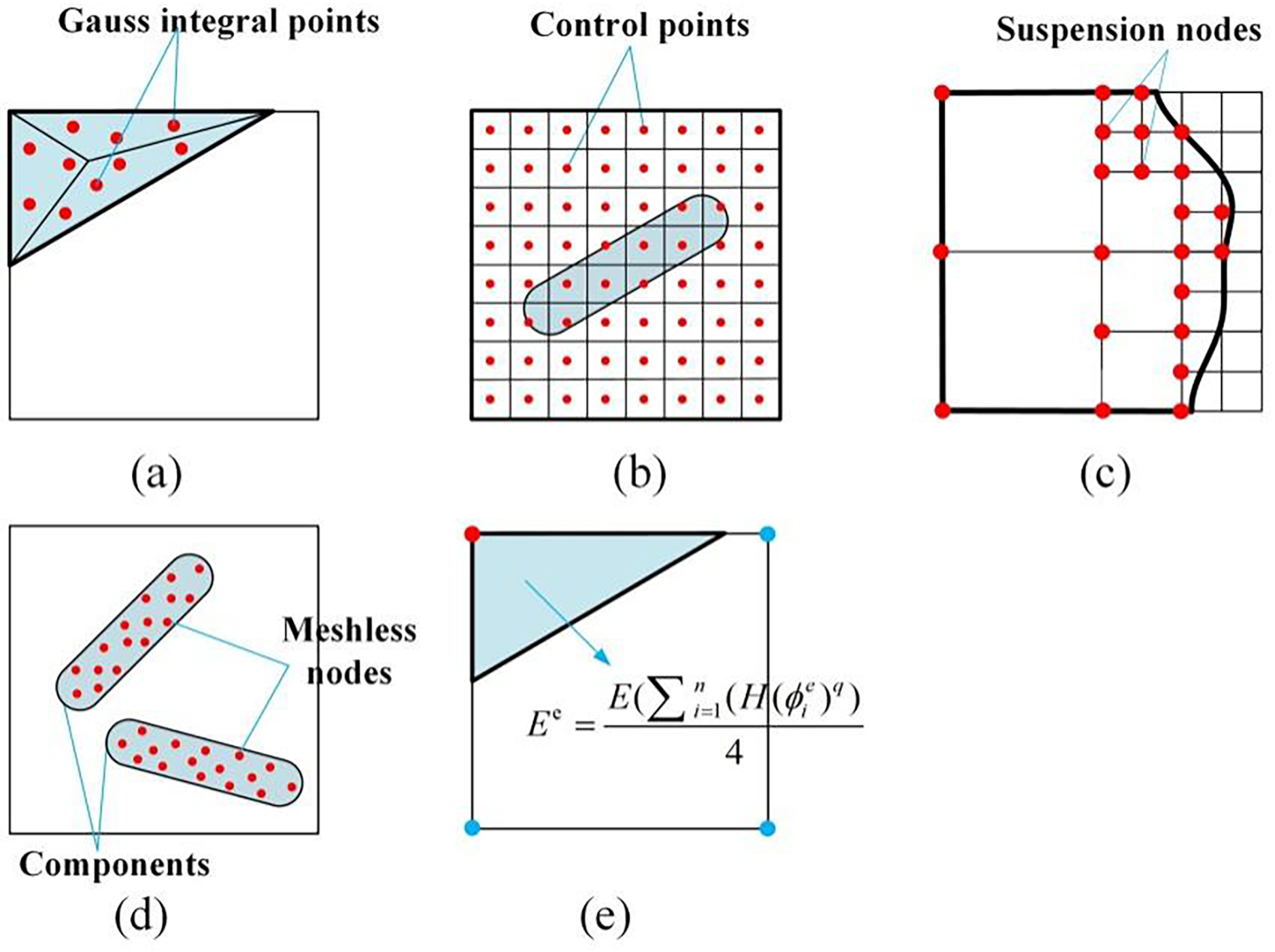
Figure 1: Finite element analysis methods for topology optimization: (a) extended finite element method (b) isogeometric analysis method (c) adaptive mesh method (d) meshless method (e) surrogate material model method

In the present work, a boundary element reconstruction model based on a surrogate material model is proposed in order to improve the accuracy of topology optimization of the MMC method. The remaining sections of the paper are organized as follows: The finite element methods applicable to the MMC method are introduced in Section 1. The accuracy problems of the surrogate material model are analyzed, and the BER model is described in Section 2. The implementation points of the BER model are elaborated in Section 3. In Section 4, the topology description function and problem formulation are presented, and the effectiveness of the proposed method is verified through several numerical examples. Section 5 provides some concluding remarks on the proposed method and its potential for future research.

2  BER Model

2.1 Accuracy Analysis of Surrogate Material Model

(1) Surrogate material model

The surrogate material model is used to define element material property based on node information. For a single material, taking the commonly used structured four-node bi-linear elements as an example, the density of the e-th element can be described as

ρe=14⁢(∑i=14(H⁡(ϕie)q)(1)

where H = H(x) is the Heaviside function and ϕie, i = 1, …, 4 are the topology description function values of element e at four nodes. q is the penalty factor (usually q = 2). The equivalent stiffness of the element can be expressed as

Ee=ρeE=E4(∑i=14(H(ϕie)q)(2)

The Eq. (2) is the surrogate material model, where E is the Young’s modulus of solid material. In order to ensure the stability of numerical implementation, H(x) is usually regularized in the following form during finite element analysis

Hε(x)={1,x>ε3(1−α)4(xτ−x33τ3)+1+α2−ε≤x≤εα,x<−ε(3)

where ε is a regularization parameter that controls the width of the smooth transition of the Heaviside function, and α is a small positive number used to simulate the stiffness of void structures in surrogate material model in order to avoid singular phenomena in the overall stiffness matrix.

(2) Accuracy of surrogate material model

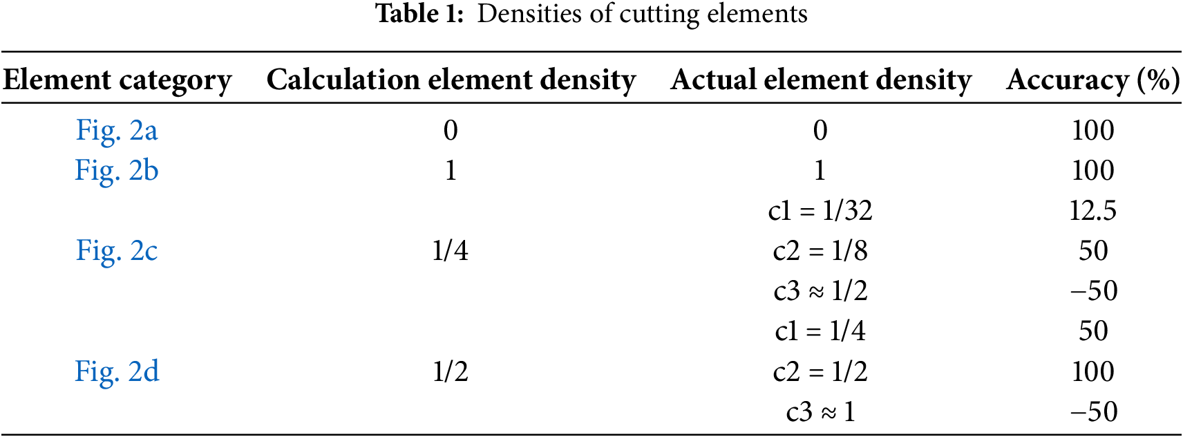
The surrogate material model obtains the element density based on the node information. When the component boundary cuts an element, different boundary cutting positions may calculate the same element density, as shown in Fig. 2. For ease of understanding, the regularization form of the Heaviside function is not considered here. The calculation element density obtained through the surrogate material model and the actual element density of the cutting elements are shown in Table 1. It can be seen that the calculation element density is just one case of the actual element density, and the variation range of actual element density under the same calculation element density is relatively large. At this time, using the calculation element density for finite element analysis may lead to significant analysis errors. In addition, the accuracy of the cutting element directly affects the calculation of the actual volume. The solid volume is often used as a constraint condition, and the results need to be input into the solver to update the design variables. Therefore, the actual volume of the cutting element will also have a certain impact on the variable update, which may affect the final structural topology.

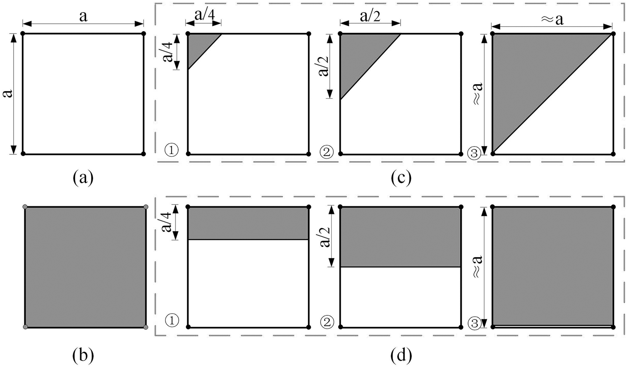
Figure 2: Schematic diagram of element cutting: (a) void element (b) solid material element. (c,d) cutting elements

2.2 Principle of BER Model

The core idea of the BER model is to perform secondary mesh partitioning and reconstruction on the boundary elements (i.e., cutting elements) to form locally dense meshes, as shown in Fig. 3a. Then, recalculate the density of the boundary elements based on the new element nodes’ information. Based on this, the two key points of the BER model are the identification of boundary elements and the strategy for calculating the density of the reconstructed elements. The identification of boundary elements can be achieved by filtering the calculation results of the surrogate material model, that is, selecting the intermediate density elements. The calculation strategy for reconstructing element density is still based on the node information, and the surrogate material model can continue to be used for the secondary calculation, but the calculation amount is large, and the implementation is complex. In this paper, a relatively simple statistical method is adopted, and the ratio of the number of solid nodes to the total number of nodes is used as the new density of the element. As shown in Fig. 3b, the calculation element density based on the original surrogate material model is 1/4. The reconstructed element has a total of 11 × 11 nodes, including 24 nodes (solid nodes) within the boundary. Therefore, the density of the element is updated to 24/121, which is more accurate than the original density. And the closer the boundary is to the nodes of the element, the more obvious the improvement of the calculation accuracy is.

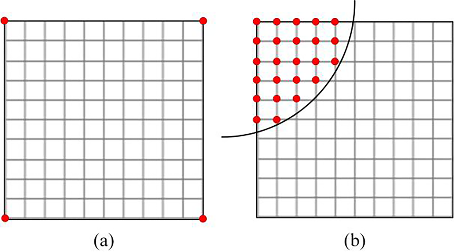
Figure 3: Element reconstruction diagram: (a) element reconstruction (b) inner nodes

2.3 Implementation Process of BER Model

The implementation of the BER model is shown in Fig. 4, which can be embedded into the existing MMC program. After the original program calculates the density of all elements using the surrogate material model, the following process is implemented:

(1)   Identify boundary elements. Based on the calculation results of the surrogate material model, where the density of non-material elements is αq and the density of solid elements is 1, the boundary elements can be identified, whose density is between αq and 1.

(2)   Reconstruct boundary elements. The same number of nodes is distributed equidistantly along both sides of the boundary element, and corresponding nodes are generated inside the boundary element to achieve mesh subdivision and reconstruction of the boundary element. The reconstruction accuracy is determined by the number of newly added nodes.

(3)   Identify nodes within the boundary. Based on all component description functions, calculate the topology values of newly added nodes, and identify the nodes within the boundaries using the Heaviside function.

(4)   Recalculate the density of boundary elements. Calculate the ratio of the number of nodes within the boundary to the total number of element nodes as the new element density for the boundary element.

(5)   Replace the density of boundary elements. Replace the new density of boundary elements in the overall stiffness matrix, and then perform finite element analysis and volume calculation.

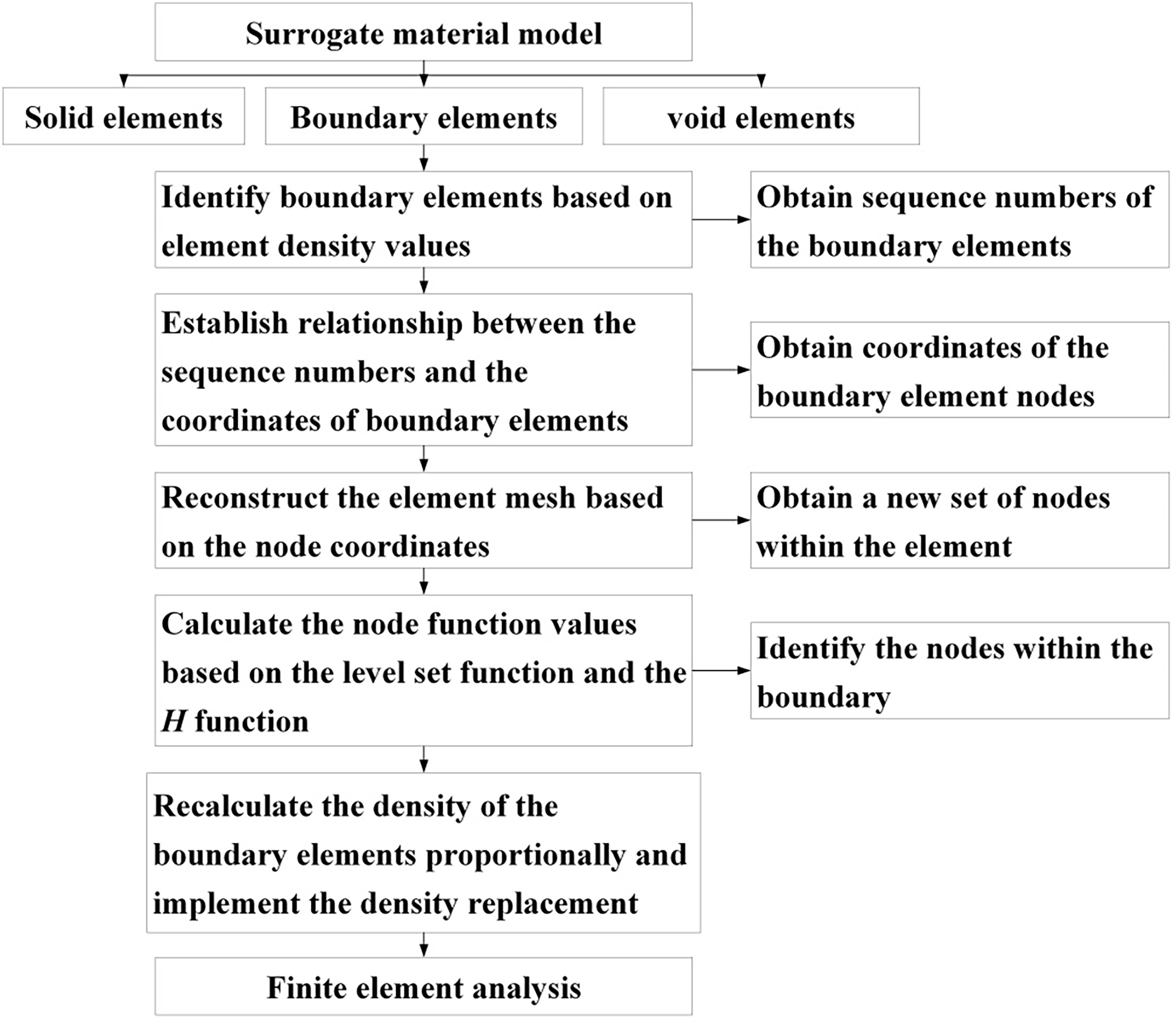
Figure 4: Implementation process

The proposal of the BER model is to obtain more accurate element density information, so as to improve the accuracy of finite element analysis, and thus enhance the accuracy of topology optimization. Compared with the global mesh refinement, which greatly increases the computational complexity of finite elements, the BER model only needs to reconstruct the boundary elements, significantly reducing the number of reconstructed elements. The newly reconstructed nodes are only used to calculate the density of boundary elements and do not participate in finite element analysis and sensitivity analysis. Therefore, the impact on the overall computational efficiency is relatively small. Moreover, the BER model can further decouple the optimization results from the background mesh.

3  Implementation Points of BER Model

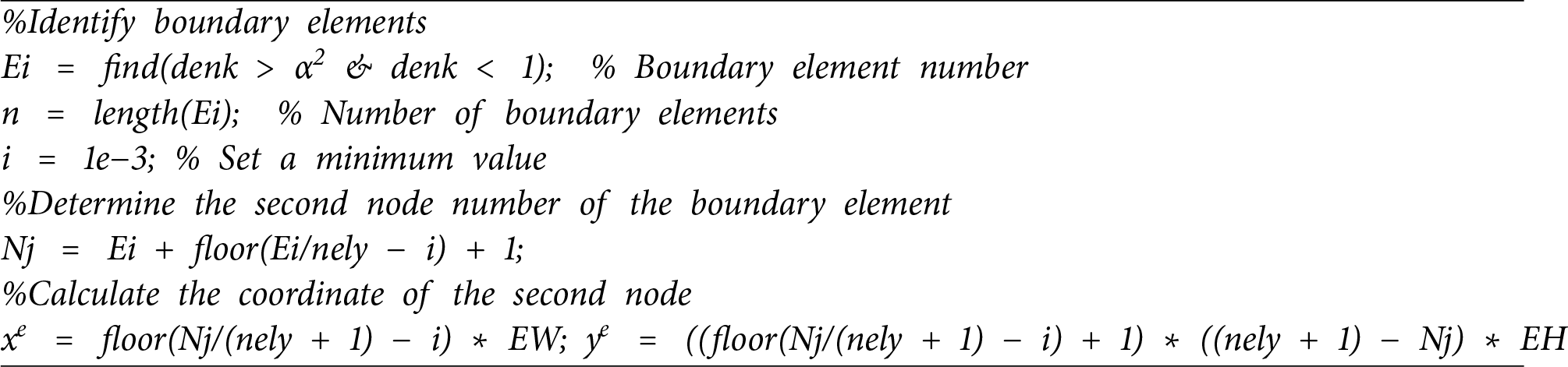
3.1 The Coordinate of Boundary Element Determination

After identifying the numbers of boundary elements, it is necessary to locate the boundary elements, that is, to determine the coordinates of boundary elements in the mesh system. In our present work, the element coordinate is determined by the element number. Taking a 3 × 3 mesh division as an example, the total number of x-direction elements is nelx = 3, and the total number of y-direction elements is nely = 3. The element length is EW and the element width is EH. The element numbers, node numbers, and coordinate origin are shown in Fig. 5. And the 2th node is chosen as the datum node.

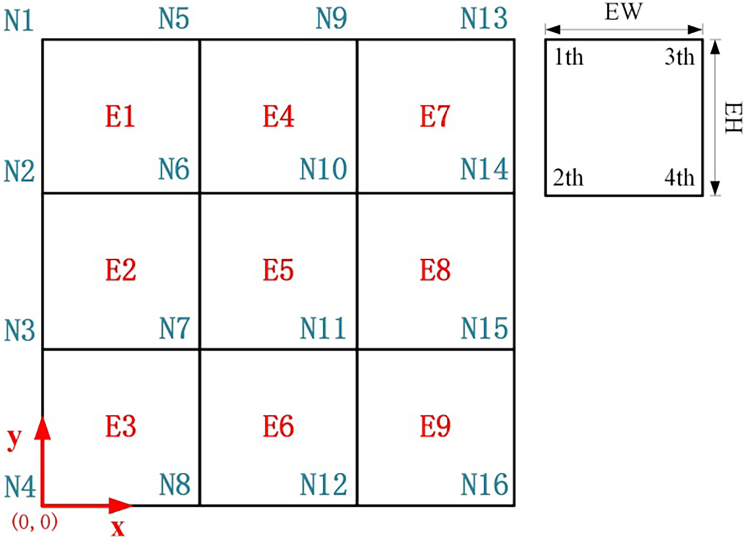
Figure 5: Element division diagram (N represents nodes and E represents elements)

The 2th node number Nj of the boundary element can be represented as

Nj=Ei+|Einely−β|integer+1(4)

where Ei is the element number, β is a very small positive value to ensure that the Eq. (4) also applies to the bottom row of elements. In this paper, β = 1 × 10−3 is taken.

The coordinates Nj(xe, ye) of the 2th node of the boundary element based on the node number can be described as

{xe=|Njnely+1−β|integer∗EWye=((|Njnely+1−β|integer+1)∗(nely+1)−Nj)∗EH(5)

The implementation code is as follows

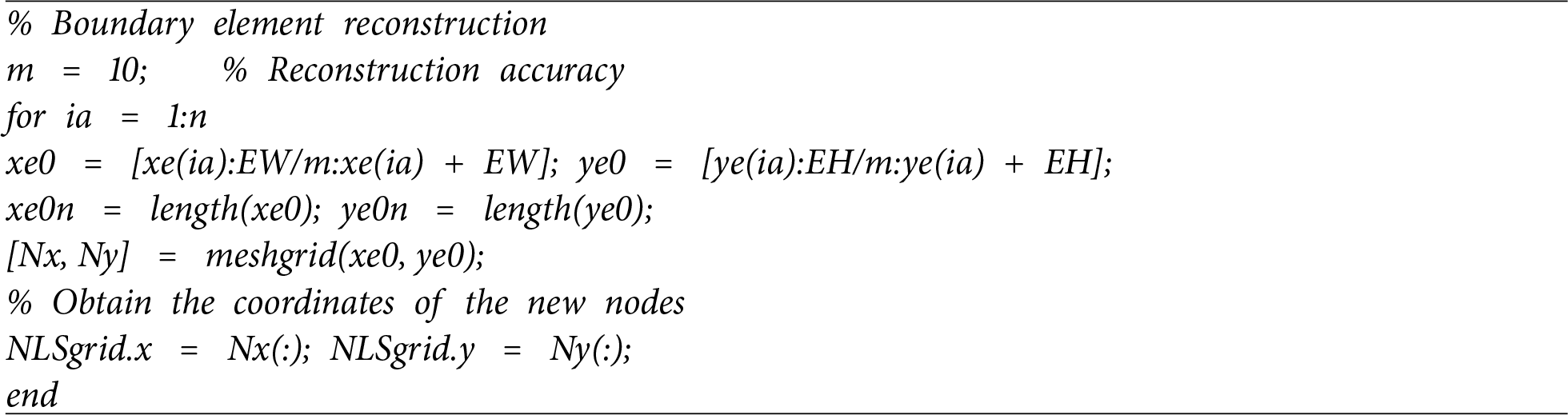
3.2 Boundary Element Reconstruction

The reconstruction accuracy is set to m (where m is an integer), and the boundary element can be reconstructed using the meshgrid function

[xN,yN]=meshgrid([xe:EWm:xe+EW],[ye:EHm:ye+EH])(6)

where xN and yN are the horizontal and vertical coordinates of all nodes of the reconstructed boundary element, respectively.

The implementation code is as follows

3.3 The Density of Boundary Element Recalculation

The topological function values of all components in the reconstructed boundary element nodes need to be calculated. Then, the topological values are mapped to the nodes through the Heaviside function (the regularization form of the Heaviside function is not necessary at this time). The number of nodes with a value of 1 in the reconstructed boundary element nodes can be counted, and the ratio of this value to the total number of element nodes is recorded as the density of the boundary element. It should be noted that in some cases, the calculated value of the new density may be 0, such as when the boundary falls on the 1st node of the element. At this time, to avoid matrix singularity, a small positive number is assigned to the new density. Finally, all the densities of the boundary elements are replaced in the overall stiffness matrix.

4  Numerical Implementation and Numerical Examples

4.1 Numerical Implementation

(1) Topology description function

According to the optimization idea of the MMC method, taking the component description of hyperelliptic equation as an example [33], the component description equation can be expressed as

ϕ(x,y)=1−(x′L)p−(y′f(x′))p(7)

with

{x′y′}=[cos⁡θsin⁡θ−sin⁡θcos⁡θ]{x−x0y−y0}(8)

where p is a relatively large positive even number (usually take p = 6). L and f(x′) represents the half-length and half-width of the i-th component, respectively. (x′, y′) and (x, y) represent the coordinates of any point in the local coordinate system and the global coordinate system, respectively, θ is the rotation angle of the component. In this paper, a quadratically varying thickness, with the component variables [x0, y0, t1, t2, t3, L], is adopted, as shown in Fig. 6, and the f(x′) is specifically expressed as

f(x′)=t1+t2−2t32L2(x′)2+t2−t12Lx′+t3(9)

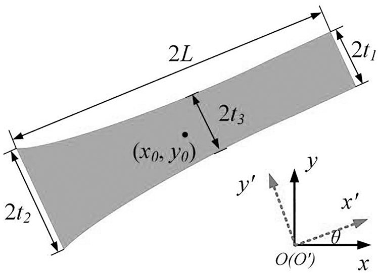
Figure 6: Geometric description of a quadratically varying thickness component

Then the structural topology description can be achieved in the following way

{ϕS(x)>0,ifx∈ΩSϕS(x)=0,ifx∈∂ΩSϕS(x)<0,ifx∈D/ΩS∂ΩS)(10)

where D represents a prescribed design domain, ΩS is the area occupied by solid materials in the design domain, ϕS(x) is the topological description function of all components, which can be expressed as

ϕS(x)=max(ϕ1e,⋅⋅⋅,ϕie,⋅⋅⋅,ϕne)(11)

where ϕie is the area occupied by i-th component, which can be described as

{ϕie(x)>0,ifx∈Ωiϕie(x)=0,ifx∈∂Ωiϕie(x)<0,ifx∈D/(Ωi∪∂Ωi)(12)

(2) Problem formulation

Taking volume as constraint and structural flexibility as objective function, the specific optimization problem formulation can be expressed as follows

FindD=((D1)T,…,(Di)T,…,(Dn)T)T,u(x)MinC=∫DH(ϕs(x,D))f⋅udV+∫Γtt⋅udSS.t.∫DH(ϕs(x,D))E:ε(u):ε(v)dV=∫DH(ϕs(x,D))f⋅vdV+∫Γtt⋅vdS,∀v∈UadV−V¯=∫DH(ϕs(x,D))dV−V¯≤0u=u¯,onΓuD⊂UD(13)

where Di is the parameters of i-th component. f and t represent body force and surface tractions, respectively. u¯ is displacement constraint, and E is elastic tensor. u(x) and v(x) are displacement field function and displacement function, respectively. H(x) represents the Heaviside function, and its regularized form is often used for achieving the continuity of the function.

Then sensitivity of objective function and constraint function can be expressed as

∂C∂a=−UT∂K∂aU=−UT(E4(∑e=1NE∑i=14q(H(ϕie))q−1∂H(ϕie)∂aks))U(14)

∂V∂a=14∑e=1NE∑i=14∂H(ϕie)∂a(15)

where a is an arbitrary design variable. ks is the element stiffness matrix, which will be used to form the overall stiffness matrix K.

The method of moving asymptotes (MMA) algorithm [34,35] is implemented to update the design variables. The information from the sensitivity analysis is used to introduce the MMA algorithm for design variable updates. Considering the feasibility of the BER model, this paper still uses a surrogate material model based on four nodes for sensitivity analysis, without considering the sensitivity of newly added nodes (i.e., the number of nodes in sensitivity analysis is still the same as that in the original overall mesh division). However, due to the reconstruction of the boundary elements density, the overall stiffness matrix K has changed. According to U = F/K, it can be inferred that the node displacement matrix U has also changed. Therefore, the sensitivity analysis of the objective function to the design variables (as shown in Eq. (14)) is different from the original calculation results, but the sensitivity of the volume constraint function to the design variables remains unchanged. In addition, the MMA algorithm also requires the volume of solid elements at each iteration, and this parameter also changes. To verify the feasibility of the proposed method, several examples are selected for analysis.

4.2 Numerical Examples

The Michell truss problem, short beam problem, and MBB beam problem are selected as examples, as shown in Fig. 7. Different mesh densities are set to demonstrate the effectiveness of the proposed method. To simplify the analysis, it is assumed that all relevant quantities in the studied problems are dimensionless, and the thickness of all design domains is set to a unit value. The Young’s modulus and Poisson’s ratio of the isotropic solid material are chosen as E = 1 and μ = 0.3, respectively. The element type is chosen as four-node bi-linear elements. The method of the MMA algorithm is implemented to update the design variables.

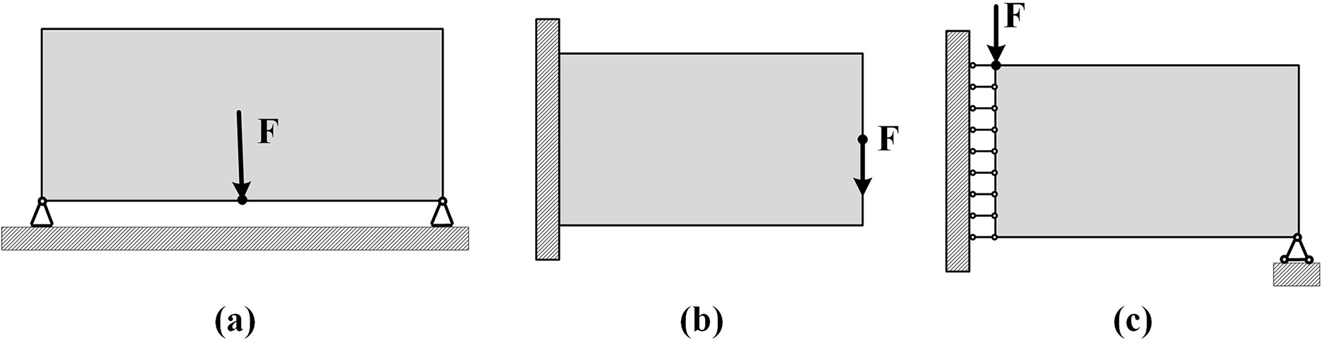
Figure 7: Problem examples: (a) Michell truss problem (b) short beam problem (c) MBB beam problem

(1) The Michell truss problem

The design domain is 2 × 1, with fixed supports at both ends of the bottom edge. A vertical load of F = 1 is applied to the midpoint of the bottom edge, and the volume constraint is set to 0.4. Three mesh densities of 80 × 40, 100 × 50, 120 × 60 are set. The Michell truss optimization results based on the surrogate material model and BRE model are shown in Fig. 8. It can be seen that the optimization results of the proposed BRE model are similar to the original surrogate material model, which verifies the effectiveness of the proposed method. Meanwhile, the structural flexibility of the optimization results of the BER model is slightly lower than that of the original surrogate material model, and the boundary is smoother.

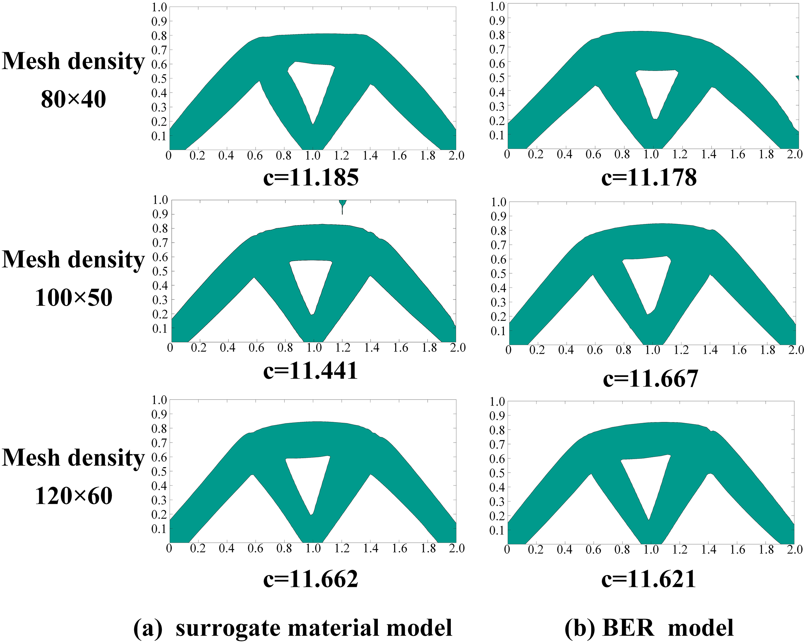
Figure 8: The optimization results of Michell truss problem

(2) The short beam problem

The design domain is 2 × 1, with the left edge fixed. A vertical load F = 1 is applied to the midpoint on the right, and the volume constraint is set to 0.4. Three mesh densities of 80 × 40, 100 × 50, 120 × 60 are set. The short beam optimization results based on the surrogate material model and BER model are shown in Fig. 9. It can be seen that the BER model can achieve good topological structures at different mesh densities, which can further reduce the mesh dependence.

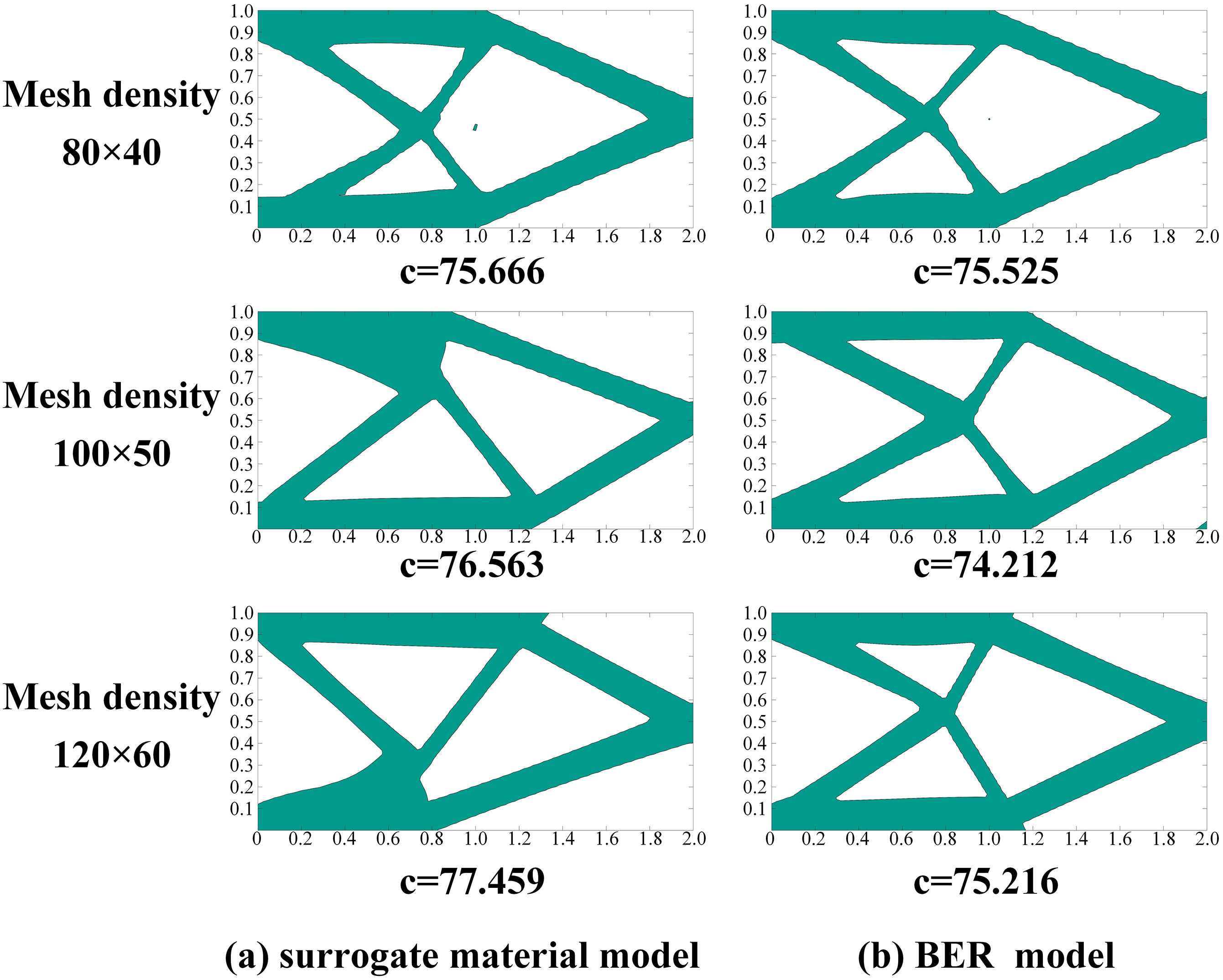
Figure 9: The optimization results of short beam problem

(3) The MBB problem

Due to the symmetry of MBB beams, half of the beam structure is selected for the design domain. The design domain is 3 × 1, with symmetrical constraints on the left side. A vertical load F = 1 is applied to the midpoint of the top edge, and the volume constraint is set to 0.4. Three mesh densities of 120 × 40, 150 × 50, 180 × 60 are set. The MBB beam optimization results based on the surrogate material model and BER model are shown in Fig. 10. It can be seen that the BER model can obtain clearer topological structure boundaries and facilitate the convergence of computational results to feasible solutions.

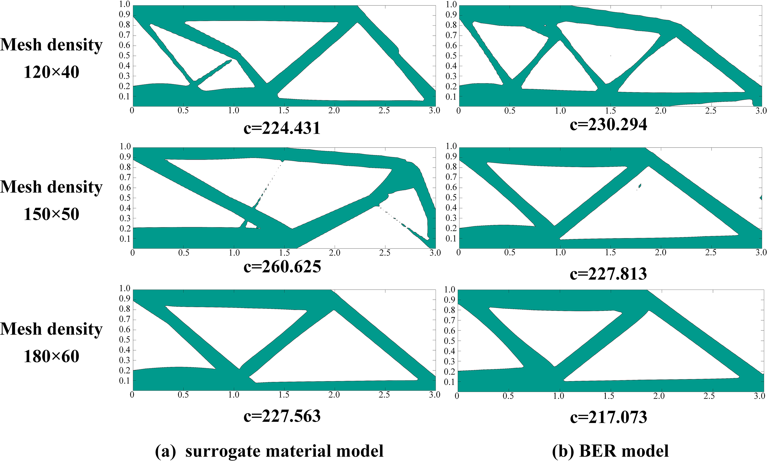
Figure 10: The optimization results of MBB problem

4.3 Analysis of Optimization Effects

(1) Iterative histories

The iterative histories of different numerical examples using surrogate material model and BER model ars shown in Figs. 11–13. It can be observed that the BER model can obtain a stable objective function value, and the number of stable iterations is almost the same as that of the surrogate material model. Moreover, the objective function value of BER model is closer under different mesh resolutions.

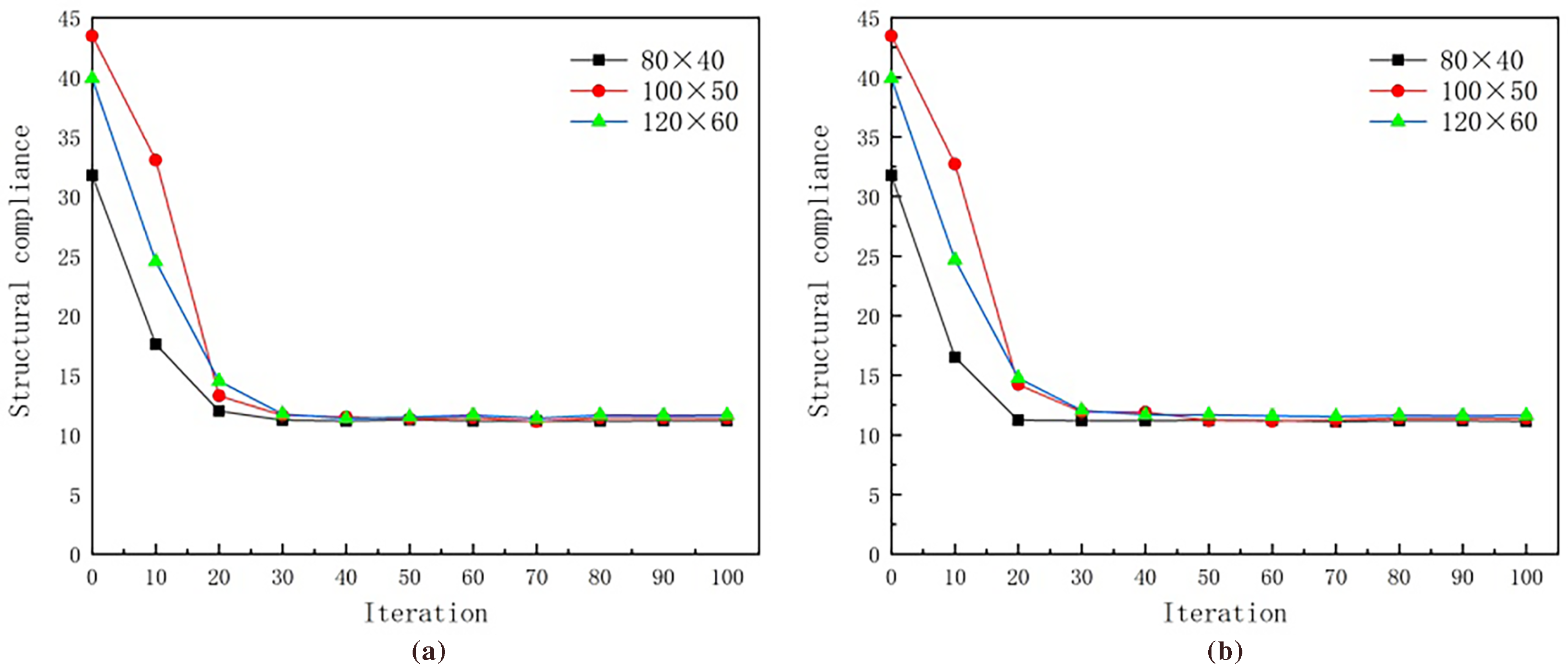
Figure 11: Iterative histories of Michell truss: (a) surrogate material model (b) BER model

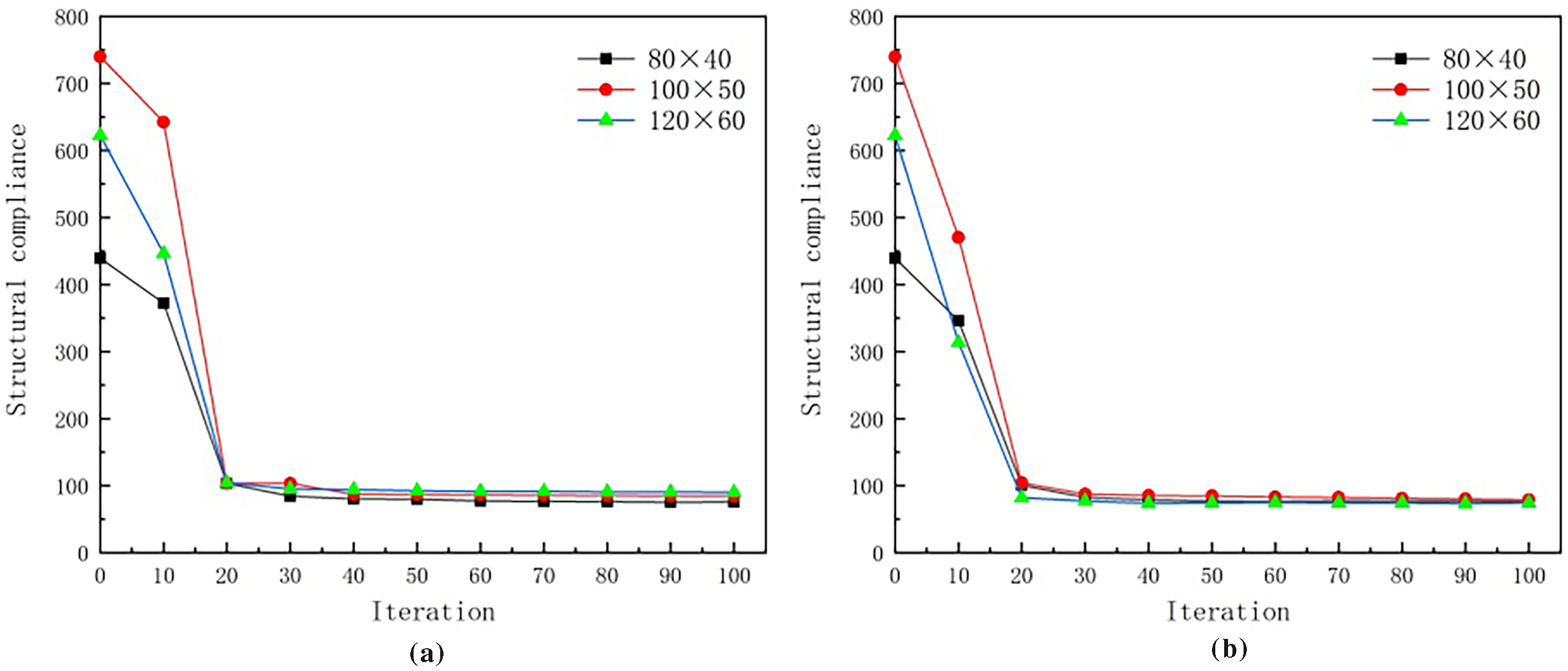
Figure 12: Iterative histories of short beam: (a) surrogate material model (b) BER model

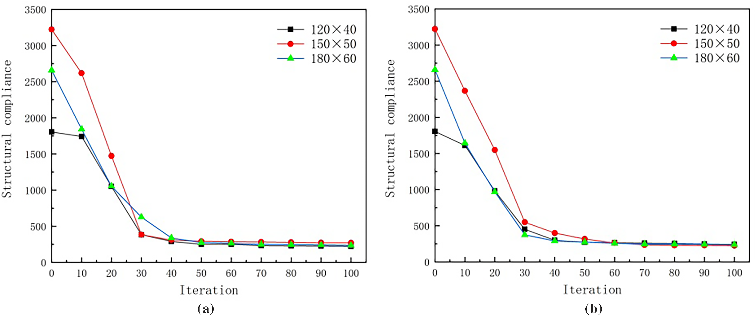
Figure 13: Iterative histories of MBB: (a) surrogate material model (b) BER model

(2) Calculation time

The calculation times using the surrogate material model and the BER model are shown in Fig. 14. As the mesh density increases, the calculation times of both models increase. Due to the addition of the process of constructing boundary elements, the calculation time required by the BER model is longer than that of the surrogate material model. In the numerical examples discussed in this paper, the calculation time required by the BER model is approximately twice that of the surrogate material model. The difference in calculation times between the two models mainly depends on the proportion of boundary elements. Generally speaking, the more complex the model is and the more boundary elements it has, the longer the calculation time will be.

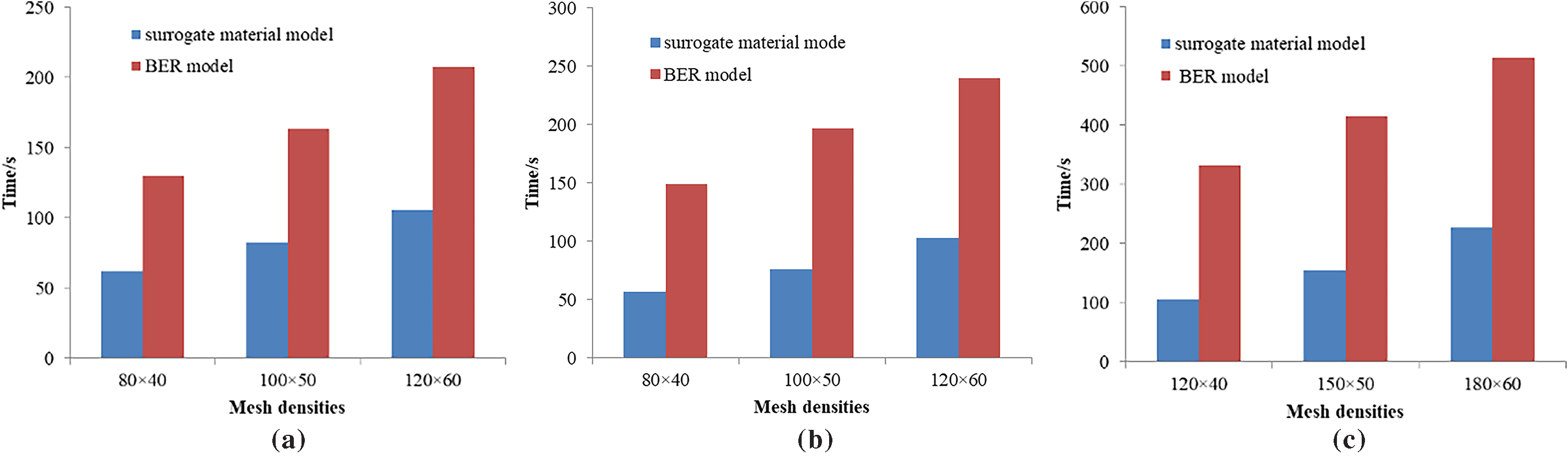
Figure 14: Comparison of calculation time: (a) Michell truss (b) Short beam (c) MBB

Analyzing the above examples, we can see that after introducing the BER model, although the computing time increases, the mesh dependence during optimization is reduced, a smoother structural topology can be obtained, and unreasonable optimization results can be improved. Moreover, the BER model also has great application potential in multi-material topology optimization.

5  Conclusion

In the present work, we introduce a new boundary element reconstruction model for the MMC topology optimization method. The proposed method focuses on the issue of boundary element density accuracy, which is cut by the boundary curve. Through processes such as element identification, element mesh reconstruction, and new node identification, the element densities are recalculated. Compared with the four-node element surrogate material model (which only calculates the element density based on four nodes), the density calculation accuracy of boundary elements has been improved. The numerical examples analysis under different mesh densities indicates that the proposed method can achieve a better structural topology, reduce the mesh dependence, and has an iteration speed similar to that of the surrogate material model, although the calculation time is longer. It is also necessary to note that the newly generated nodes do not participate in the finite element analysis, thereby effectively avoiding a significant increase in computational cost. Moreover, the proposed method is easy to implement and can be integrated into existing algorithms. Due to its more precise boundary element density values, the proposed method also has potential application in multi-material structure optimization, which is the subsequent work of our study.

Acknowledgement: Not applicable.

Funding Statement: This work was supported by the Science and Technology Research Project of Henan Province (242102241055), the Industry-University-Research Collaborative Innovation Base on Automobile Lightweight of “Science and Technology Innovation in Central Plains” (2024KCZY315), and the Opening Fund of State Key Laboratory of Structural Analysis, Optimization and CAE Software for Industrial Equipment (GZ2024A03-ZZU).

Author Contributions: Study conception and design: Zhao Li, Hongyu Xu; data collection: Zhao Li, Shuai Zhang; analysis of results: Zhao Li, Jintao Cui, Xiaofeng Liu; draft manuscript preparation: Zhao Li, Hongyu Xu. All authors reviewed the results and approved the final version of the manuscript.

Availability of Data and Materials: Data will be made available on request.

Ethics Approval: Not applicable.

Conflicts of Interest: The authors declare no conflicts of interest to report regarding the present study.

References

1. Tang T, Wang L, Zhu M, Zhang H, Dong J, Yue W, et al. Topology optimization: a review for structural designs under statics problems. Materials. 2024;17(23):5970. doi:10.3390/ma17235970. [Google Scholar] [PubMed] [CrossRef]

2. Li P, Shen X, Dong S, Fang Y. Topology optimization methods and its applications in aerospace: a review. Struct Multidiscip Optim. 2025;68(5):105. doi:10.1007/s00158-025-04030-x. [Google Scholar] [CrossRef]

3. Bendsøe MP, Kikuchi N. Generating optimal topologies in structural design using a homogenization method. Comput Methods Appl Mech Eng. 1988;71(2):197–224. doi:10.1016/0045-7825(88)90086-2. [Google Scholar] [CrossRef]

4. Bendsøe MP. Optimal shape design as a material distribution problem. Struct Optim. 1989;1(4):193–202. doi:10.1007/bf01650949. [Google Scholar] [CrossRef]

5. Mei Y, Wang X. A level set method for structural topology optimization and its applications. Adv Eng Softw. 2004;35(7):415–41. [Google Scholar]

6. Guo X, Zhang W, Zhong W. Doing topology optimization explicitly and geometrically—a new moving morphable components based framework. J Appl Mech. 2014;81(8):081009. doi:10.1115/1.4027609. [Google Scholar] [CrossRef]

7. Li Z, Xu H, Zhang S. A comprehensive review of explicit topology optimization based on moving morphable components (MMC) method. Arch Comput Methods Eng. 2024;31(5):2507–36. doi:10.1007/s11831-023-10053-8. [Google Scholar] [CrossRef]

8. Yang H, Huang J. An explicit structural topology optimization method based on the descriptions of areas. Struct Multidiscip Optim. 2020;61(3):1123–56. doi:10.1007/s00158-019-02414-4. [Google Scholar] [CrossRef]

9. Lu C, Chen W, Liu S. A moving morphable component (MMC)-based topology optimization method for underwater sound absorption materials using a mixed finite element formulation. Struct Multidiscip Optim. 2025;68(7):1–17. doi:10.1007/s00158-025-04057-0. [Google Scholar] [CrossRef]

10. Li Z, Xu H, Zhang S. Moving morphable component (MMC) topology optimization with different void structure scaling factors. PLoS One. 2024;19(1):e0296337. doi:10.1371/journal.pone.0296337. [Google Scholar] [PubMed] [CrossRef]

11. Li Z, Xu H, Zhang S, Cui J, Liu X. Multi-material structures topology optimization for thin-walled tube used by vehicles under static load: a review. Arch Comput Methods Eng. 2025;61:1–41. doi:10.1007/s11831-025-10285-w. [Google Scholar] [CrossRef]

12. Abdi M, Wildman R, Ashcroft I. Evolutionary topology optimization using the extended finite element method and isolines. Eng Optim. 2014;46(5):628–47. doi:10.1080/0305215x.2013.791815. [Google Scholar] [CrossRef]

13. Rostami SAL, Kolahdooz A, Zhang J. Robust topology optimization under material and loading uncertainties using an evolutionary structural extended finite element method. Eng Anal Bound Elem. 2021;133:61–70. doi:10.1016/j.enganabound.2021.08.023. [Google Scholar] [CrossRef]

14. Hughes TJR, Cottrell JA, Bazilevs Y. Isogeometric analysis: CAD, finite elements, NURBS, exact geometry and mesh refinement. Comput Methods Appl Mech Eng. 2005;194(3941):4135–95. doi:10.1016/j.cma.2004.10.008. [Google Scholar] [CrossRef]

15. Lin D, Gao L, Gao J. The Lagrangian-Eulerian described particle flow topology optimization (PFTO) approach with isogeometric material point method. Comput Methods Appl Mech Eng. 2025;440:117892. doi:10.1016/j.cma.2025.117892. [Google Scholar] [CrossRef]

16. Zhang X, Gao L, Xiao M, Gao J. T-splines-based panel method for aerodynamic topology optimization of engineering shell structures using isogeometric analysis. Comput Methods Appl Mech Eng. 2025;444:118154. doi:10.1016/j.cma.2025.118154. [Google Scholar] [CrossRef]

17. Gao J, Xiao M, Zhang Y, Gao L. A comprehensive review of isogeometric topology optimization: methods, applications and prospects. Chin J Mech Eng. 2020;33(1):87. doi:10.1186/s10033-020-00503-w. [Google Scholar] [CrossRef]

18. Yang A, Wang S, Luo N, Xiong T, Xie X. A space-preserving data structure for isogeometric topology optimization in B-splines space. Struct Multidiscip Optim. 2022;65(10):281. doi:10.1007/s00158-022-03358-y. [Google Scholar] [CrossRef]

19. Gai Y, Zhu X, Zhang YJ, Hou W, Hu P. Explicit isogeometric topology optimization based on moving morphable voids with closed B-spline boundary curves. Struct Multidiscip Optim. 2020;61(3):963–82. doi:10.1007/s00158-020-02553-z. [Google Scholar] [CrossRef]

20. Xie X, Yang A, Jiang N, Zhao W, Liang Z, Wang S. Adaptive topology optimization under suitably graded THB-spline refinement and coarsening. Int J Numer Methods Eng. 2021;122(20):5971–98. doi:10.1002/nme.6780. [Google Scholar] [CrossRef]

21. Zhou J, Zhao G, Zeng Y, Li G. A novel topology optimization method of plate structure based on moving morphable components and grid structure. Struct Multidiscip Optim. 2024;67(1):8. doi:10.1007/s00158-023-03719-1. [Google Scholar] [CrossRef]

22. Zhang W, Jiang Q, Feng W, Youn SK, Guo X. Explicit structural topology optimization using boundary element method-based moving morphable void approach. Int J Numer Methods Eng. 2021;122(21):6155–79. doi:10.1002/nme.6786. [Google Scholar] [CrossRef]

23. Suvin VS, Ooi ET, Song C, Natarajan S. Adaptive scaled boundary finite element method for hydrogen assisted cracking with phase field model. Theor Appl Fract Mech. 2024;134:104690. doi:10.1016/j.tafmec.2024.104690. [Google Scholar] [CrossRef]

24. Gaddam SK, Natarajan S, Kanjarla AK. Octree-based scaled boundary finite element approach for polycrystal RVEs: a comparison with traditional FE and FFT methods. Comput Methods Appl Mech Eng. 2025;438:117864. doi:10.1016/j.cma.2025.117864. [Google Scholar] [CrossRef]

25. Zhang Y, Ge W, Zhang Y, Zhao Z, Zhang J. Topology optimization of hyperelastic structure based on a directly coupled finite element and element-free Galerkin method. Adv Eng Softw. 2018;123:25–37. doi:10.1016/j.advengsoft.2018.05.006. [Google Scholar] [CrossRef]

26. Patel VG, Rachchh NV. Meshless method—review on recent developments. Mater Today Proc. 2020;26:1598–603. [Google Scholar]

27. Sousa L, Oliveira S, Vidal C, Cavalcante-Neto J. A truly meshless approach to structural topology optimization based on the direct meshless local petrov-galerkin (DMLPG) method. Struct Multidiscip Optim. 2024;67(7):110. doi:10.1007/s00158-024-03813-y. [Google Scholar] [CrossRef]

28. Zhang W, Yuan J, Zhang J, Guo X. A new topology optimization approach based on moving morphable components (MMC) and the ersatz material model. Struct Multidiscip Optim. 2016;53(6):1243–60. doi:10.1007/s00158-015-1372-3. [Google Scholar] [CrossRef]

29. Li Z, Hu X, Chen W. Moving morphable curved components framework of topology optimization based on the concept of time series. Struct Multidiscip Optim. 2023;66(1):19. doi:10.1007/s00158-022-03472-x. [Google Scholar] [CrossRef]

30. Wang L, Shi D, Zhang B, Li G, Liu P. Real-time topology optimization based on deep learning for moving morphable components. Autom Constr. 2022;142:104492. doi:10.1016/j.autcon.2022.104492. [Google Scholar] [CrossRef]

31. Otsuka K, Dong S, Kuzuno R, Sugiyama H, Makihara K. Moving morphable multi components introducing intent of designer in topology optimization. AIAA J. 2023;61(4):1720–34. [Google Scholar]

32. Mao C, Huang X, Lu G, Choong PFM, Tse KM. Advanced topology optimisation for porous hip implants: bridging in silico models and in vitro tests. J Mech Behav Biomed Mater. 2025;170:107031. doi:10.1016/j.jmbbm.2025.107031. [Google Scholar] [PubMed] [CrossRef]

33. Li Z, Xu H, Zhang S, Cui J, Liu X. Design of multiple materials structure based on an explicit and implicit hybrid topology optimization method. Sci Rep. 2025;15(1):19591. [Google Scholar] [PubMed]

34. Svanberg K. The method of moving asymptotes—a new method for structural optimization. Int J Numer Methods Eng. 1987;24(2):359–73. doi:10.1002/nme.1620240207. [Google Scholar] [CrossRef]

35. Mo K, Guo D, Wang H. Iterative reanalysis approximation-assisted moving morphable component-based topology optimization method. Int J Numer Methods Eng. 2020;121(22):5101–22. doi:10.1002/nme.6514. [Google Scholar] [CrossRef]