Siphon-Based Divide-and-Conquer Policy for Enforcing Liveness on Petri Net Models of FMS Suffering from Deadlocks or Livelocks

1  Introduction

Nowadays, due to very fast and ever-changing market demands, automated, flexible and agile manufacturing systems are required to answer these demands quickly and efficiently. Deadlocks are an unacceptable system behavior in flexible manufacturing systems (FMS) and occur due to the improper allocation of shared resources such as machines, robots, AGVs, conveyors, etc. In a deadlock state, the whole FMS stops completely, spoiling the use of resources and leading to devastating effects on the operation of these systems [1]. Therefore, in an FMS, the occurrences of deadlocks are not acceptable. A lot of efforts have been put into the study of deadlocks and their resolution in FMS. Petri nets (PN) [2] have been widely utilized for the study of deadlocks/livelocks, control, and scheduling of FMS [3]. PN based studies to tackle deal with the deadlock problems in FMSs, can be split into three groups as deadlock avoidance [4–8], deadlock detection and recovery [9–11], and deadlock prevention [12–16]. Deadlock prevention policies are preferred over the other methods because the necessary computations are carried out off-line and once. In these methods, to prevent deadlocks/livelocks from occurring, an uncontrolled Petri net model (UPNM) of an FMS prone to deadlocks/livelocks is used to compute a liveness-enforcing supervisor (LES) containing a set of control places (CPs) (also called monitors). CPs contain input arcs, output arcs and initial markings. The controlled live PNM is constructed by merging the LES with the UPNM. A live PN assures operations without deadlocks and livelocks [17–21].

Structural analysis and reachability graph (RG) analysis are two common analysis methods for the study of deadlock problems. Structural analysis is used for the synthesis of LESs by using special PN objects such as siphons or resource-transitions circuits [12,22–25]. The number of siphons grows exponentially w.r.t. the size of a PNM. The RG analysis of a PN in the deadlock prevention studies fully reflects the behavior of an FMS [13,26–29], but requires complete or partial enumeration of the state space [30–34]. In theory, the size of an RG may grow exponentially w.r.t. the size of the PNM. RG-based liveness enforcing methods may provide high permissive behavior, optimal or near-optimal solutions, while in general, structural analysis-based methods provide suboptimal solutions in most cases, because some legal markings cannot be reached. The liveness-enforcing methods relying on special PN objects are applicable to a certain class of PNs.

To evaluate the computed PN-based LESs, there are three criteria: behavioral permissiveness, structural complexity, and computational complexity [35]. The behavioral permissiveness is evaluated by the number of reachable good (legal) markings of the controlled PNM (CPNM). The live CPNM is called to be optimal (maximally permissive) when it is possible to reach all good markings. However, the live CPNM is called suboptimal when some legal markings are not reachable within the live CPNM. The structural complexity is generally evaluated by the number of CPs in an LES. The structural complexity is directly affected by whether or not a CP contains weighted input/output arcs [36]. Therefore, ordinary CPs, whose input/output arc weights are all one, are preferred over the generalized CPs, whose some input/output arc weights are greater than one. Therefore, a low structural complexity provides fewer numbers and a simpler structure of CPs, which means lower implementation expenses in terms of both hardware and software costs. Computational complexity is related to the efficiency of a liveness-enforcing control method. Low computational complexity implies that a control policy can be obtained within a reasonable time, and it can be applied to large-scale PNMs. Therefore, these three criteria have been followed by the research community around the world as three lines of research. In this paper, we are mainly concerned with reducing the computational complexity of computing LESs for large-scale industrial FMSs. In doing so, we also aim to obtain very high permissiveness and low structural complexity.

Divide-and-conquer (DaC) based approaches [37–39] have been proposed to reduce the computational complexity for large-scale systems. In the DaC paradigm, to compute an LES for a UPNM suffering from deadlocks/livelocks, the UPNM is divided into several subnets, which are smaller and easier to handle. When an LES consisting of a set of CPs is computed by using the subnets, a live CPNM is constructed by merging the LES with the UPNM. Therefore, the use of the DaC paradigm in the PN-based liveness enforcing in FMS can be considered as a special direction of research to deal with the computational complexity problem. The work reported in [37] may be considered as the very first DaC method for PN-based liveness enforcing in FMS. In [37], a UPNM is divided into an autonomous subnet, an idle subnet, and several small subnets, i.e., toparchies. An LES, called toparch, is computed for each toparchy. It was shown that the resulting net, called monarch, by composing the toparches derived for the toparchies, can serve as an LES for the given UPNM. It was claimed in [37] that the DaC-based method of [37] computationally outperforms the methods reported in [12,13,26,40]. The method proposed in [37] deals only with dividing the UPNM into a set of subnets, and the method proposed in [12] is used to compute CPs for the toparchies.

A DaC-based deadlock prevention method was proposed in [39], where decomposition techniques are proposed for deadlock prevention within a class of PNs used to model FMSs. The proposed method first decomposes a PN into two subnets. Next, for each subnet, LESs are computed. After that, two controlled subnets are merged, and another LES is also synthesized from the merged net. Then, the live CPNM is obtained. This policy is based on the RG analysis of the subnets only. There are two drawbacks of this method: it is applicable to S3PR nets only, and a maximally permissive LES cannot be obtained.

Another DaC method was proposed in [38] for the computation of PN-based LESs for FMSs. A UPNM of an FMS prone to deadlock/livelock is divided into a set of connected subnets by considering all combinations of shared resources. The set of connected subnets contains both live and non-live subnets. Then, subnets with deadlock problems are used to compute an LES to enforce liveness on the UPNM. This technique makes use of RG analysis of a given UPNM and all its subnets, which is carried out by using INA [41]. This PN tool is rather slow when enumerating the whole RG. Besides, INA cannot handle large RGs having a few million states. This fact restricts the application of the method of [38] to realistic FMS with very large RGs. Another drawback is that this method requires considering all live and non-live subnets, which may be a very time-consuming task for large PNMs with a lot of shared resources. The proposed policy in this paper improves the DaC technique of [38] in two ways. The first improvement involves the computation of subnets utilizing a novel and unprecedented approach. To do this, firstly, strict minimal siphons (SMS) of the reduced PNM are computed. Then, from these SMSs, the complementary set of SMSs is computed. With the union of these two sets, supersets of siphons of the reduced PNM are computed. Finally, the set of subnets of the reduced PNM is obtained by applying the PN reduction rules [40] on the superset of siphons. It is important to note that all these subnets suffer from deadlocks. The second improvement is related to the use of the PN tool. In this study, we propose to use TINA [42] as a better alternative, which is much faster than INA. Thanks to the technique reported in [43] for the computation of RGs, live zones (LZs), and deadlock zones (DZs) of a UPNM suffering from deadlocks/livelocks using TINA, the policy proposed in this paper can tackle RGs having more than 100 million states.

A novel siphon-based divide-and-conquer (SbDaC) policy for the computation of LESs for FMSs suffering from deadlocks or livelocks is proposed in this paper. The SbDaC policy is applicable to all classes of PNMs used to model FMSs suffering from deadlock/livelock problems currently accessible in the relevant literature. The SbDaC policy takes a UPNM of an FMS with deadlock/livelock problems as input and provides an LES consisting of a set of CPs to enforce liveness. Thus, the CPNM constructed by merging the LES with the UPNM is live. From a behavioral permissiveness perspective, in general, the CPNM provides optimal or near-optimal behaviour. Since the computed LES contains only ordinary CPs, whose input/output arcs have the weight of 1, the structural complexity of the computed LES is low. Even though it is necessary to compute all SMSs and the RGs of a given UPNM and all its subnets, the SbDaC policy is straightforward, easy to use, and effective. The application of the SbDaC policy for FMS control assures its live operation and high resource utilization and system throughput. Five examples are considered from the literature to show the applicability of the SbDaC policy. In the relevant liveness-enforcing literature, PNMs with very large RGs having more than 100 million states are very rare due to the computational complexity and the demand for very high computational facilities. Since three of the examples used in this paper have very large RGs, this fact highlights the importance, efficiency and applicability of the proposed SbDaC policy.

The paper is organized as follows. Section 2 provides 1. a list of important classes of PNs related to FMS currently available in the literature, 2. some definitions on siphon, complementary set of a siphon and superset of a siphon, 3. PN reduction rules, 4. explanation of RG of a PNM suffering from deadlocks/livelocks. The proposed SbDaC policy is explained in Section 3. Examples used to show the applicability of the SbDaC policy are provided in the next section. Section 5 presents the conclusions.

2  Basic Concepts

In this paper, the reader is expected to have the basic background information related to PNs [2], and some well-known techniques such as PN reduction, siphon computation, and control synthesis. This section serves as a brief reminder of such concepts used in this paper. In this section, firstly, the classes of PNs related to FMS are highlighted. Then, the concepts related to siphons used in this paper are explained. Next, PN reduction rules are considered. Finally, the RG of an FMS suffering from deadlock problems is studied to unveil the philosophy behind the RG-based deadlock prevention strategy.

2.1 Classes of Petri Nets Related to FMS

The SbDaC policy is applicable to all classes of PNs related to FMS used for the deadlock/livelock studies. Well-known classes of PNs related to FMS include the following nets [44]: PPNs (production Petri nets), S3PR (systems of simple sequential processes with resources) nets, ES3PR (extended systems of simple sequential processes with resources) nets, LS3PR (linear systems of simple sequential processes with resources) nets, ELS3PR nets (an extended LS3PR net), GS3PR (generalized systems of simple sequential processes with resources) nets, GLS3PR (generalized linear systems of simple sequential processes with resources) nets, S3PGR2 (system of simple sequential processes with general resource requirements) nets, S3PMR (systems of simple sequential processes with multiple resources) nets, WS3PR (weighted system of simple sequential processes with resources) nets, WS3PSR (weighted system of simple sequential processes with several resources) nets, S4PR (simple systems of simple sequential processes with resources) nets, S4R (systems of simple sequential processes with shared resources) nets, S*PR nets, PNR (process nets with resources) nets, RCN-merged nets (resource control nets-merged nets), ERCN-merged nets (extended resource control nets-merged nets), ERCN∗-merged (well-behaved extended resource control nets-merged) nets, G-Systems, Augmented marked graph (AMG) nets, AEMG (augmented extended marked graph) nets, HMG (hierarchical marked graph) nets, HAMG (hierarchical augmented marked graph) nets.

2.2 Siphon, Complementary Set of a Siphon and Superset of a Siphon

P-vector I is called a place invariant (P-invariant) iff I ≠ 0 and IT[N] = 0T hold. P-invariant I is a P-semiflow, if its every entry is non-negative. The set ||I|| = {p ∈ P | I[p] ≠ 0} is the support of a vector I. A siphon is a non-empty subset of places S, i.e., S ⊆ P is a siphon iff •S ⊆ S•. A trap is a non-empty subset of places S, i.e., S ⊆ P is a trap iff S• ⊆ •S. A siphon (trap) is minimal iff there is no siphon (trap) contained in it as a proper subset [12]. A siphon is said to be a strict minimal siphon (SMS) iff it is minimal and does not contain a marked trap. A siphon refers to a strict minimal siphon (SMS) in this paper unless otherwise stated. If a siphon is the support of a P-semiflow and if it is initially marked, then it can never be emptied. Siphons are very important structural objects that are adopted in deadlock prevention/liveness-enforcing policies for both generalized and ordinary PNMs of FMSs.

For the example S3PR given in Fig. 1 [45], we have the set of activity places PA = {p2, p3, p4, p6, p7, p8, p9, p10}, the set of idle (sink/source) places P0 = {p1, p5}, the set of resource places PR = {p11, p12, p13, p14, p15}.

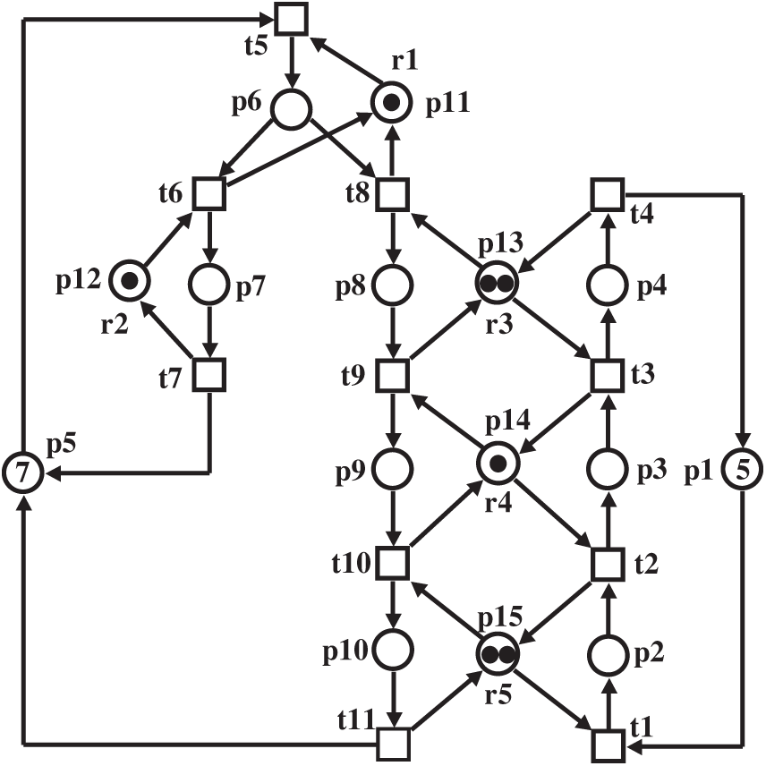
Figure 1: An S3PR net from [45]

Let S be the set of siphons. For the S3PR given in Fig. 1, there are three siphons S = {S1, S2, S3}. S1 = {p3, p10, p14, p15}, S2 = {p4, p9, p13, p14}, S3 = {p4, p10, p13, p14, p15}. These siphons are depicted in Fig. 2. •S1 = {t2, t3, t10, t11}, S1• = {t1, t2, t3, t9, t10, t11}: •S1 ⊆ S1•. •S2 = {t3, t4, t9, t10}, S2• = {t2, t3, t4, t8, t9, t10}: •S2 ⊆ S2•. •S3 = {t2, t3, t4, t9, t10, t11}, S3• = {t1, t2, t3, t4, t8, t9, t10, t11}: •S3 ⊆ S3•.

Figure 2: Three SMSs S = {S1, S2, S3} of the S3PR net shown in Fig. 1. (a) S1 = {p3, p10, p14, p15}; (b) S2 = {p4, p9, p13, p14}; (c) S3 = {p4, p10, p13, p14, p15}

Let S ∈ S be an SMS in a Petri net N, where S = SA ∪ SR, SR = S ∩ PR = S\SA, and SA = S ∩ PA = S\SR. For example, for S1 = {p3, p10, p14, p15} we have S1R = S1 ∩ PR = S1\SA = {p14, p15}, S1A = S1 ∩ PA = S1\SR = {p3, p10}; for S2 = {p4, p9, p13, p14} we have S2R = S2 ∩ PR = S2\SA = {p13, p14}, S2A = S2 ∩ PA = S2\SR = {p4, p9}; for S3 = {p4, p10, p13, p14, p15} we have S3R = S3 ∩ PR = S3\SA = {p13, p14, p15}, S3A = S3 ∩ PA = S3\SR = {p4, p10}.

For r ∈ PR, H(r) = ••r ∩ PA, the activity (operation) places that use r is called the set of holders of r. For a set of resources PR = {r1, r2, …, rm}, the set of activity (operation) places whose operations require these resources is denoted by H(r1) ∪ H(r2) ∪ … ∪ H(rm) [4]. For example, for the S3PR given in Fig. 1, as we have PR = {p11, p12, p13, p14, p15}, the set of holders of r ∈ PR are as follows H(p11) = {p6}, H(p12) = {p7}, H(p13) = {p4, p8}, H(p14) = {p3, p9}, H(p15) = {p2, p10}. This means that place p6 uses p11, place p7 uses p12, places p4 and p8 use p13, places p3 and p9 use p14, places p2 and p10 use p15.

[S] = ∪r∈SRH(r)\S is called the complementary set of siphon S. For example, for the three siphons S = {S1, S2, S3}: S1 = {p3, p10, p14, p15}, S2 = {p4, p9, p13, p14}, S3 = {p4, p10, p13, p14, p15} of the S3PR shown in Fig. 2, the corresponding complementary sets [S] = {[S1], [S2], [S3]} are

[S1] = (H(p14) ∪ H(p15))\S1

[S1] = ({p3, p9} ∪ {p2, p10})\{p3, p10, p14, p15}

[S1] = {p2, p3, p9, p10}\{p3, p10, p14, p15}

[S1] = {p2, p9}

[S2] = (H(p13) ∪ H(p14))\S2

[S2] = ({p4, p8} ∪ {p3, p9})\{p4, p9, p13, p14}

[S2] = {p3, p4, p8, p9}\{p4, p9, p13, p14}

[S2] = {p3, p8}

[S3] = (H(p13) ∪ H(p14) ∪ H(p15))\S3

[S3] = ({p4, p8} ∪ {p3, p9} ∪ {p2, p10})\{p4, p10, p13, p14, p15}

[S3] = {p2, p3, p4, p8, p9, p10}\{p4, p10, p13, p14, p15}

[S3] = {p2, p3, p8, p9}

The complementary sets of siphons [S1], [S2], and [S3] are depicted in Fig. 3. ∀S ∈ S, S^ = S ∪ [S] is defined as the superset of a siphon S. In an ordinary PN, the sum of tokens that exist in a siphon S and the complementary set [S] of S is constant. This means that when a siphon S loses a token, the complementary set [S] of S gains a token and vice versa [12]. Thus, S^ = S ∪ [S] forms the support of a minimal P-invariant. When all tokens that exist in a siphon S flow into the complementary set [S] of S, S will be empty [12]. For the example S3PR shown in Fig. 1, the superset of SMSs S, S^ = {S1^, S2^, S3^} = {S1 ∪ [S1], S2 ∪ [S2], S3 ∪ [S3]} is computed as follows: S1^ = S1 ∪ [S1] = {p3, p10, p14, p15} ∪ {p2, p9} = {p2, p3, p9, p10, p14, p15}. S2^ = S2 ∪ [S2] = {p4, p9, p13, p14} ∪ {p3, p8} = {p3, p4, p8, p9, p13, p14}. S3^ = S3 ∪ [S3] = {p4, p10, p13, p14, p15} ∪ {p2, p3, p8, p9} = {p2, p3, p4, p8, p9, p10, p13, p14, p15}. The supersets of SMSs, S1^, S2^, and S3^ are depicted in Fig. 4. Although the concepts considered in the previous paragraphs on siphons, the complementary set of a siphon, the set of holders of r and the superset of a siphon S are explained using an S3PR net example, they are also applicable to other classes of PNs related to FMS used for the deadlock/livelock studies currently available in the literature.

Figure 3: The complementary set of siphons [S] = {[S1], [S2], [S3]} of the S3PR net shown in Fig. 1. (a) [S1] = {p2, p9}; (b) [S2] = {p3, p8}; (c) [S3] = {p2, p3, p8, p9}

Figure 4: The superset of SMSs S, S^ = {S1^, S2^, S3^} of the S3PR net shown in Fig. 1. (a) S1^; (b) S2^; (c) S3^

2.3 PN Reduction Rules

The LES synthesis approach proposed in this paper makes use of RGs of a given PNM of an FMS suffering from deadlocks/livelocks. To reduce the computation burden, it is important to use the PN reduction approach for PNs with large RGs as explained in [40]. A set of reduction rules include the elimination of self-loop transitions or places, the fusion of parallel transitions or places, fusion of series transitions or places. The PN reduction rules are used to obtain the properties of a complex PNM, while the concerned properties, i.e., boundedness, reversibility and liveness, are preserved. When an LES is computed by using the reduced PNM, it can then be used for the original PNM to enforce liveness. In this paper, PN reduction rules are not only used to obtain the reduced PNM of a given UPNM suffering from deadlock/livelock problems, but also used to obtain reduced subnets of the uncontrolled net model. For example, Fig. 5 depicts the reduced S3PR net obtained by using the PN reduction rules. The RG of the S3PR net has 380 markings while its reduced net has only 27 markings.

Figure 5: Reduced S3PR net

2.4 Deadlock/Livelock Studies Based on Reachability Graph (RG) of PNs

In [40], the reachability graph (RG) of an FMS with deadlock problems is divided into a deadlock zone (DZ) and a live zone (LZ). The DZ contains deadlocks, first-met bad markings (FBMs), and bad markings (BMs). An FBM is a marking within the DZ and it represents the first entry from the LZ to the DZ. FBMs and BMs inevitably lead to deadlocks. Deadlocks, FBMs and BMs are all considered to be illegal markings. The LZ consists of all legal markings, from where the initial marking M0 can be reached. At a deadlock marking no transition can fire. Therefore, it has no successor, which means that this is a dead situation in a system. At a BM, there are firable transitions, i.e., it has successor markings, but the initial marking M0 cannot be reached from a BM. An FBM is a marking whose ancestor marking is in the LZ, but it is in the DZ. A good marking (GM) can reach M0, and its successors can also reach it. A dangerous marking (DM) can reach M0, but at least one of its successors cannot reach M0. Both good and dangerous markings in the RG must be kept in the controlled system for the sake of optimal control purposes. Therefore, they are considered legal markings. In an RG, when all FBMs are made unreachable by control places (CPs), the system can never go into the DZ from the LZ. In this case, the controlled system runs solely in the LZ, and it is live [46]. Detailed explanations of the deadlock/livelock studies based on RG of PNs are available in [43].

3  A Siphon-Based Divide-and-Conquer (SbDaC) Synthesis Policy for Liveness-Enforcing in FMS

In this section, a novel siphon-based divide-and-conquer (SbDaC) synthesis policy is presented for the computation of LESs consisting of CPs with ordinary arcs for classes of PNs related to FMS suffering from deadlocks or livelocks. Algorithm 1 shows the proposed SbDaC synthesis policy. It is assumed that an uncontrolled bounded PNM (UPNM) of an FMS prone to deadlocks or livelocks is given as input. The PN reduction approach is used to reduce large PNMs to carry out required computations easily, as described in a previous section. The reduced PNM (RPNM) is obtained from the given UPNM (N, M0). If the RG of the UPNM is not very large, then the original UPNM can also be used. Given a UPNM of an FMS with deadlock/livelock problems, the aim is to compute an LES consisting of a set of CPs for the UPNM. To compute the LES for an FMS, the RPNM of the system is split into a set of subnets SN = {S1N, S2N, …, SnN} by using SMSs S = {S1, S2, …, Sn} of the RPNM. SMSs are computed by using INA [41]. To obtain a set of subnets SN = {S1N, S2N, …, SnN}, firstly, the set of SMSs S = {S1, S2, …, Sn} of the RPNM is computed. Secondly, the complementary set of siphons [S] = {[S1], [S2], …, [Sn]} is computed. Next, the superset of SMSs S, S^ = {S1^, S2^, …, Sn^} = {S1 ∪ [S1], S2 ∪ [S2], …, Sn ∪ [Sn]} is computed. These three steps are explained in detail in the previous sections. Finally, the subnets SN = {S1N, S2N, …, SnN} are obtained from the superset of SMSs S by using the PN reduction approach. Then, the RGs of all subnets SN = {S1N, S2N, …, SnN} are computed, and the numbers of states in the RGs, LZs and DZs of all subnets are defined. These two sets of computations are carried out by using TINA [42] with the guidance of the method explained in [43]. It is important to note that all subnets SN = {S1N, S2N, …, SnN} suffer from deadlocks. Therefore, it is necessary to consider each subnet starting from the smallest one to the largest one to make it live by computing CPs. Some CPs computed for smaller subnets may be used in the larger subnets.

The next step involves the ordering of subnets SN = {S1N, S2N, …, SnN} from the smallest one to the largest one based on the number of activity places of each subnet. This process provides new sets of subnets as follows: SN1, the set of subnets with 1 activity place, SN2, the set of subnets with 2 activity places, SN3, the set of subnets with 3 activity places, …, up to the set of subnets with the maximum number of activity places. CPs are computed starting from the smallest nonempty set of subnets to make them live. The RG of each subnet is taken into account with its DZ and LZ. Markings of the DZ (deadlocks, FBMs, BMs) are treated as BMs. They are made unreachable by using the simplified invariant-based control method [40]. In the computations, only the marked activity places of a BM are utilized. To stop the activity places of the BM from being marked, the activity places of the BM are characterized as a place invariant (PI). Therefore, the sum of tokens within the activity places of the PI must be one token fewer than its current value within the BM. A PI is realized by a CP. In this study, the simplified version [40] of the method proposed in [47], is utilized to synthesize a CP from a PI. Computed CPs are included within the set of CPs ψ.

The computation of CPs is carried out with larger subnets. If the set of marked activity places of a PI of any previously computed CP from the set ψ is a subset of the considered subnet SNi,j, i.e., [PI]map ⊆ [SNi,j]ap, then the partially controlled subnet SNi,j, called pCSNi,j, is obtained by merging all previously computed CPs whose [PI]map ⊆ [SNi,j]ap, with SNi,j. If the partially controlled SNi,j, i.e., pCSNi,j, is live, then the next subnet is considered. If it is not live, then a new set of CPs is also synthesized for the considered subnet SNi,j. This process continues until all subnets are live. Finally, all computed CPs are included within the set ψ. Next, the redundancy test [48] is conducted for all computed CPs by using the RPNM to find the set of necessary CPs ψ = {C1, C2, …, Cm}. Finally, the live CPNM (Nc, Mc) is constructed by merging the necessary CPs ψ = {C1, C2, …, Cm} with the PNM (N, M0).

The set of necessary CPs ψ = {C1, C2, …, Cm} is structurally simple because CPs consist of only ordinary input/output arcs, i.e., the weight of all arcs within the set of necessary CPs ψ = {C1, C2, …, Cm} is 1. This is because in the synthesis of CPs, each coefficient li [47] is set to one. On the contrary, when a CP is merged with the UPNM to forbid a selected BM, this process may lead to loss of some legal markings, as indicated in [27]. This is because in some FMS deadlock/livelock prevention problems, some legal markings could not be reachable when disabling the illegal ones with the added CPs. From the behavioral permissiveness point of view, except for some generalized PNMs with a lot of highly shared resources, the behavioral permissiveness of the obtained controlled models provides an optimal or near-optimal solution.

[PI]map is called the set of marked activity places of a BM in a DZ. For instance, let us assume, a deadlock is reached when both marked activity places p3 and p8 contain two tokens, i.e., μ3 = 2 and μ8 = 2. Then, the PI used to prevent the reachability of this deadlock marking is defined as μ3 + μ8 ≤ 3. Therefore, the set of marked activity places of this PI is [PI]map = {p3, p8}.

[SNi,j]ap is called the set of activity places of a subnet SNi,j. Recall that i is the number of activity places in a subnet and j is the current subnet in the set SNi. For example, [SN4,1]ap = {p3, p4, p5, p8} means that the first subnet within the set of subnets with four activity places contains the activity places p3, p4, p5 and p8.

The proposed SbDaC policy requires both the complete enumeration of siphons (SMSs) of a given UPNM and the generation of RGs of the given UPNM, the reduced PNM and the subnets. It utilizes well-known techniques such as the siphon computation of the reduced PN, by using INA [41], PN reduction rules [40], the RG computation of the subnets and the reduced PN, by using TINA [42], the computation of the number of states of within the LZ and the DZ, the computation of the markings of all states in the DZ of the subnets and the reduced PN by using TINA as explained in [43], the redundancy test [48] for the computed CPs, the liveness analysis of the CPNM (Nc, Mc) by using TINA. In addition, BMs of a DZ are defined as PIs, and they are implemented by CPs using the simplified version [40] of the method in [47]. Some of these individual components have been extensively studied and implemented in the popular Petri net tools currently available in the literature. Therefore, further studies may be conducted to reveal the performance comparison between the ones utilized in this paper and the currently available Petri net tools such as Charlie [49,50].

In this study, the RG analysis and computations of both the LZs and the DZs, and the computations of siphons are conducted by using a computer with an Intel(R) Core i5-6200U 2.3 GHz CPU using 12 GB of RAM, running Windows 10 operating system. In addition, the RG analysis and computations of both the LZs and the DZs of the three realistic examples having a very large number of states in their RGs are carried out by another computer with an AMD Ryzen 7 7800X3D 8-Core Processor 4.2 GHz CPU using 128 GB of RAM, running Windows 10 operating system. Conducted experimental studies show that the SbDaC policy is applicable to large-scale FMS-oriented PNMs.

4  Examples

In this section, an illustrative S3PMR net and three realistic example nets, namely two S3PR nets and an S3PGR2 net, which belong to different FMS-oriented classes, PNs are considered from the literature to show the applicability of the SbDaC policy. Especially, the three realistic examples contain very large RGs.

4.1 Illustrative Example—S3PMR Net

Fig. 6 depicts an S3PMR net of an FMS. Originally, this net model was firstly introduced in [51]. Compared with the original S3PMR net, the one considered here, shown in Fig. 6, has two additional arcs, namely Pre(t9, p26) and Post(p26, t8), to make place p9 bounded. This S3PMR net suffers from deadlocks and consists of 26 places, P = {p1–p26} and 20 transitions, T = {t1–t20}. In this UPNM, we have PR = {p20–p26}, PA = {p2, p3, p4, p6–p13, p15, p16–p19}, and P0 = {p1, p5, p14}.

Figure 6: S3PMR net of an FMS from [51] with added two arcs prone to deadlocks

Input: The S3PMR net (UPNM) (N, M0) of an FMS suffering from deadlocks depicted in Fig. 6. The RG of the S3PMR net has 4691 markings and 17,196 transitions. The LZ and the DZ have 3581 and 1110 states, respectively. Optimally controlled live PNM must reach 3581 good markings.

Step 1. The set of CPs is defined as ψ. ψ: = {}.

Step 2. The reduced S3PMR net is depicted in Fig. 7. The RG of the reduced S3PMR net contains 1692 markings and 5964 transitions. The LZ and the DZ have 1110 and 582 states, respectively.

Figure 7: Reduced S3PMR net

Note that for brevity in steps 3, 4, and 5, place names are provided without the prefix “p”.

Step 3. By using INA, twenty-four SMSs S = {S1, S2, …, S24} are computed as follows: S1 = {20, 21, 22, 23, 24, 26}, S2 = {17, 18, 21, 22, 23, 24, 26}, S3 = {10, 11, 20, 21, 23, 24, 26}, S4 = {10, 11, 17, 18, 21, 23, 24, 26}, S5 = {9, 12, 20, 21, 22, 24, 26}, S6 = {9, 12, 17, 18, 21, 22, 24, 26}, S7 = {9, 10, 11, 20, 21, 24, 26}, S8 = {9, 10, 11, 17, 18, 21, 24, 26}, S9 = {16, 23, 24, 26}, S10 = {9, 16, 24, 26}, S11 = {7, 8, 20, 21, 22, 23}, S12 = {7, 8, 12, 20, 21, 22}, S13 = {7, 8, 17, 18, 21, 22, 23}, S14 = {7, 8, 12, 17, 18, 21, 22}, S15 = {7, 8, 10, 11, 20, 21}, S16 = {3, 20, 21, 22, 23, 26}, S17 = {3, 17, 18, 21, 22, 23, 26}, S18 = {16, 22, 23}, S19 = {2, 8, 20, 21, 22, 23, 24}, S20 = {2, 8, 12, 20, 21, 22, 24}, S21 = {2, 8, 17, 18, 21, 22, 23, 24}, S22 = {2, 8, 12, 17, 18, 21, 22, 24}, S23 = {2, 8, 10, 11, 20, 21, 24}, S24 = {2, 8, 10, 11, 17, 18, 21, 24}.

Step 4. The twenty-four complementary set of siphons [S] = {[S1], [S2], …, [S24]} are computed as follows: [S1] = {2, 3, 6, 7, 8, 9, 10, 12, 15, 16, 17}, [S2] = {2, 3, 7, 8, 9, 10, 12, 15, 16}, [S3] = {2, 3, 6, 7, 8, 9, 15, 16, 17}, [S4] = {2, 3, 7, 8, 9, 15, 16}, [S5] = {2, 3, 6, 7, 8, 10, 16, 17}, [S6] = {2, 3, 7, 8, 10, 16}, [S7] = {2, 3, 6, 7, 8, 16, 17}, [S8] = {2, 3, 7, 8, 16}, [S9] = {2, 3, 8, 9, 15}, [S10] = {2, 3, 8}, [S11] = {6, 10, 12, 15, 16, 17}, [S12] = {6, 10, 16, 17}, [S13] = {10, 12, 15, 16}, [S14] = {10, 16}, [S15] = {6, 17}, [S16] = {6, 7, 8, 9, 10, 12, 15, 16, 17}, [S17] = {7, 8, 9, 10, 12, 15, 16}, [S18] = {12, 15}, [S19] = {6, 7, 10, 12, 15, 16, 17}, [S20] = {6, 7, 10, 16, 17}, [S21] = {7, 10, 12, 15, 16}, [S22] = {7, 10, 16}, [S23] = {6, 7, 16, 17}, [S24] = {7, 16}.

Step 5. The supersets of SMSs S, S^ = {S1^, S2^, …, S24^} = {S1 ∪ [S1], S2 ∪ [S2], …, S24 ∪ [S24]} are computed as follows: S1^ = S1 ∪ [S1] = {20, 21, 22, 23, 24, 26} ∪ {2, 3, 6, 7, 8, 9, 10, 12, 15, 16, 17} = {2, 3, 6, 7, 8, 9, 10, 12, 15, 16, 17, 20, 21, 22, 23, 24, 26}. S2^ = S2 ∪ [S2] = {17, 18, 21, 22, 23, 24, 26} ∪ {2, 3, 7, 8, 9, 10, 12, 15, 16} = {2, 3, 7, 8, 9, 10, 12, 15, 16, 17, 18, 21, 22, 23, 24, 26}. S3^ = S3 ∪ [S3] = {10, 11, 20, 21, 23, 24, 26} ∪ {2, 3, 6, 7, 8, 9, 15, 16, 17} = {2, 3, 6, 7, 8, 9, 10, 11, 15, 16, 17, 20, 21, 23, 24, 26}. S4^ = S4 ∪ [S4] = {10, 11, 17, 18, 21, 23, 24, 26} ∪ {2, 3, 7, 8, 9, 15, 16} = {2, 3, 7, 8, 9, 10, 11, 15, 16, 17, 18, 21, 23, 24, 26}. S5^ = S5 ∪ [S5] = {9, 12, 20, 21, 22, 24, 26} ∪ {2, 3, 6, 7, 8, 10, 16, 17} = {2, 3, 6, 7, 8, 9, 10, 12, 16, 17, 20, 21, 22, 24, 26}. S6^ = S6 ∪ [S6] = {9, 12, 17, 18, 21, 22, 24, 26} ∪ {2, 3, 7, 8, 10, 16} = {2, 3, 7, 8, 9, 10, 12, 16, 17, 18, 21, 22, 24, 26}. S7^ = S7 ∪ [S7] = {9, 10, 11, 20, 21, 24, 26} ∪ {2, 3, 6, 7, 8, 16, 17} = {2, 3, 6, 7, 8, 9, 10, 11, 16, 17, 20, 21, 24, 26}. S8^ = S8 ∪ [S8] = {9, 10, 11, 17, 18, 21, 24, 26} ∪ {2, 3, 7, 8, 16} = {2, 3, 7, 8, 9, 10, 11, 16, 17, 18, 21, 24, 26}. S9^ = S9 ∪ [S9] = {16, 23, 24, 26} ∪ {2, 3, 8, 9, 15} = {2, 3, 8, 9, 15, 16, 23, 24, 26}. S10^ = S10 ∪ [S10] = {9, 16, 24, 26} ∪ {2, 3, 8} = {2, 3, 8, 9, 16, 24, 26}. S11^ = S11 ∪ [S11] = {7, 8, 20, 21, 22, 23} ∪ {6, 10, 12, 15, 16, 17} = {6, 7, 8, 10, 12, 15, 16, 17, 20, 21, 22, 23}. S12^ = S12 ∪ [S12] = {7, 8, 12, 20, 21, 22} ∪ {6, 10, 16, 17} = {6, 7, 8, 10, 12, 16, 17, 20, 21, 22}. S13^ = S13 ∪ [S13] = {7, 8, 17, 18, 21, 22, 23} ∪ {10, 12, 15, 16} = {7, 8, 10, 12, 15, 16, 17, 18, 21, 22, 23}. S14^ = S14 ∪ [S14] = {7, 8, 12, 17, 18, 21, 22} ∪ {10, 16} = {7, 8, 10, 12, 16, 17, 18, 21, 22}. S15^ = S15 ∪ [S15] = {7, 8, 10, 11, 20, 21} ∪ {6, 17} = {6, 7, 8, 10, 11, 17, 20, 21}. S16^ = S16 ∪ [S16] = {3, 20, 21, 22, 23, 26} ∪ {6, 7, 8, 9, 10, 12, 15, 16, 17} = {3, 6, 7, 8, 9, 10, 12, 15, 16, 17, 20, 21, 22, 23, 26}. S17^ = S17 ∪ [S17] = {3, 17, 18, 21, 22, 23, 26} ∪ {7, 8, 9, 10, 12, 15, 16} = {3, 7, 8, 9, 10, 12, 15, 16, 17, 18, 21, 22, 23, 26}. S18^ = S18 ∪ [S18] = {16, 22, 23} ∪ {12, 15} = {12, 15, 16, 22, 23}. S19^ = S19 ∪ [S19] = {2, 8, 20, 21, 22, 23, 24} ∪ {6, 7, 10, 12, 15, 16, 17} = {2, 6, 7, 8, 10, 12, 15, 16, 17, 20, 21, 22, 23, 24}. S20^ = S20 ∪ [S20] = {2, 8, 12, 20, 21, 22, 24} ∪ {6, 7, 10, 16, 17} = {2, 6, 7, 8, 10, 12, 16, 17, 20, 21, 22, 24}. S21^ = S21 ∪ [S21] = {2, 8, 17, 18, 21, 22, 23, 24} ∪ {7, 10, 12, 15, 16} = {2, 7, 8, 10, 12, 15, 16, 17, 18, 21, 22, 23, 24}. S22^ = S22 ∪ [S22] = {2, 8, 12, 17, 18, 21, 22, 24} ∪ {7, 10, 16} = {2, 7, 8, 10, 12, 16, 17, 18, 21, 22, 24}. S23^ = S23 ∪ [S23] = {2, 8, 10, 11, 20, 21, 24} ∪ {6, 7, 16, 17} = {2, 6, 7, 8, 10, 11, 16, 17, 20, 21, 24}. S24^ = S24 ∪ [S24] = {2, 8, 10, 11, 17, 18, 21, 24} ∪ {7, 16} = {2, 7, 8, 10, 11, 16, 17, 18, 21, 24}

Step 6. The subnets SN = {S1N, S2N, …, S24N} depicted in Fig. 8 are obtained from the superset of SMSs S, S^ = {S1^, S2^, …, S24^} by using the PN reduction rules.

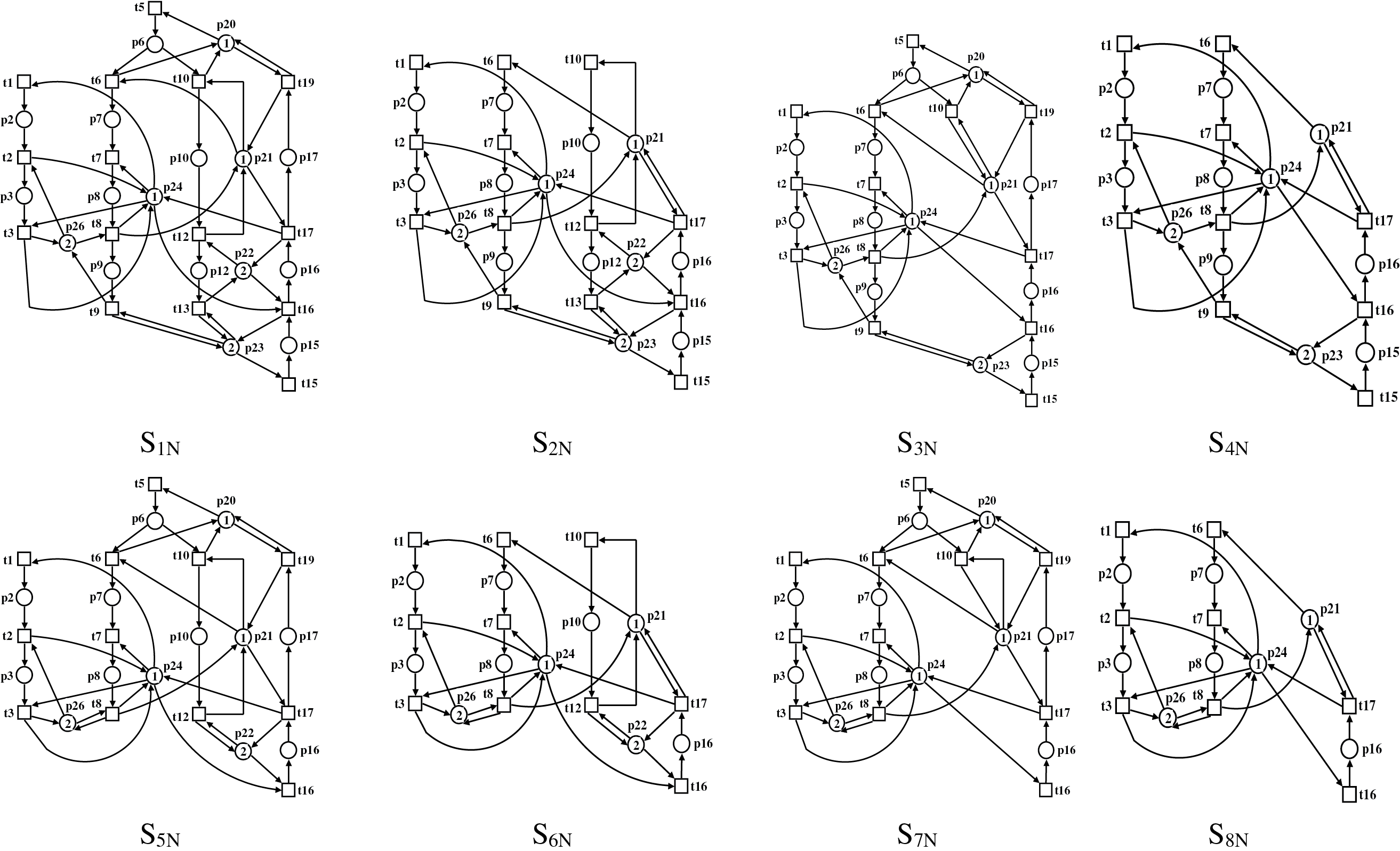
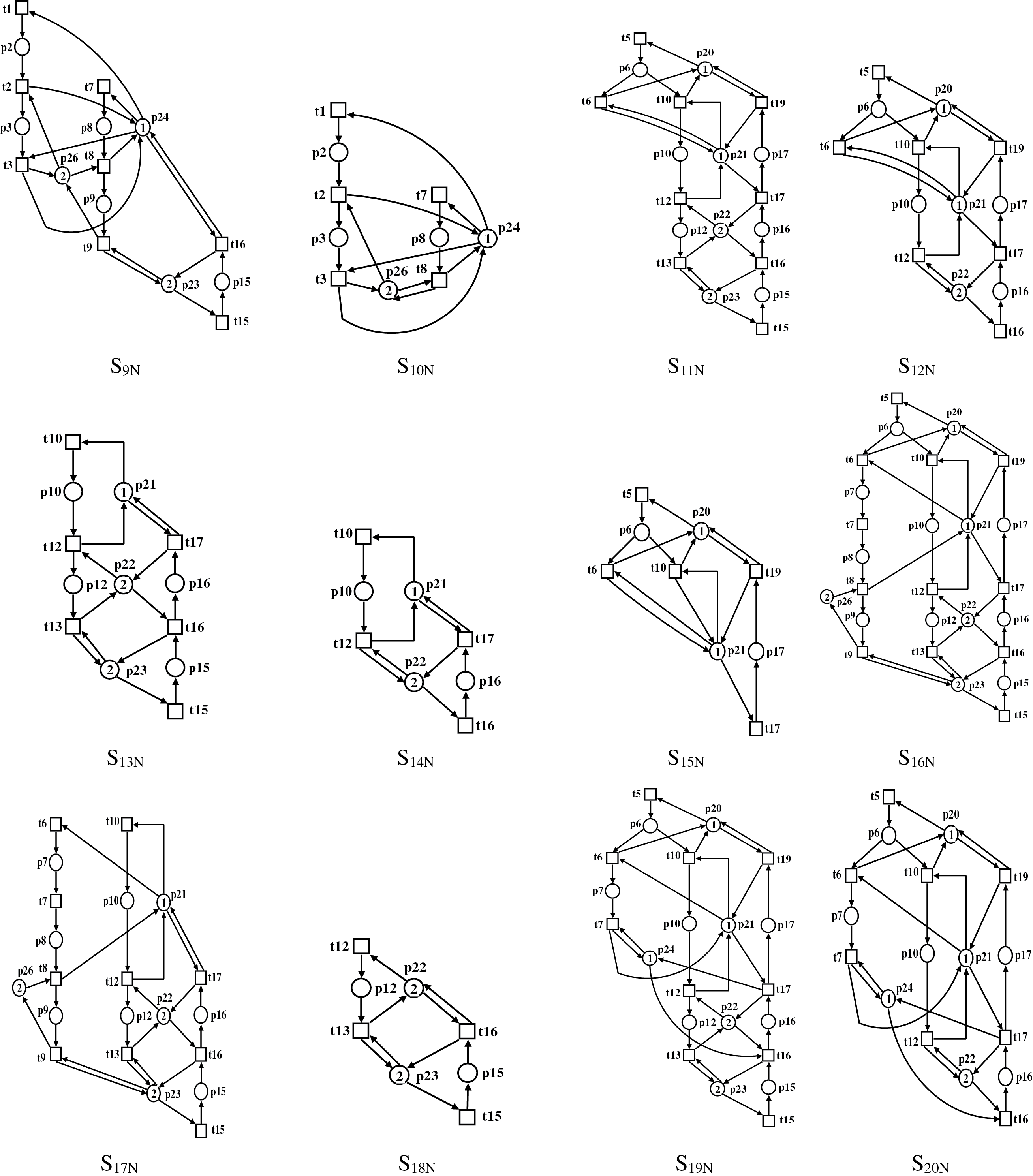
Figure 8: The subnets SN = {S1N, S2N, …, S24N}

Step 7. The RGs of all subnets SN = {S1N, S2N, …, S24N} are computed, and the numbers of states in the RGs, LZs and DZs of all subnets are defined. The number of markings in the RG, DZ and LZ of the subnets SN = {S1N, S2N, …, S24N} are depicted in Table 1.

Step 8. The set of activity places of each subnet SN = {S1N, S2N, …, S24N} is defined as depicted in Table 2. For instance, the set of activity places of subnets S14N, S13N, and S6N are as follows [S14N]ap = {p10, p16}, [S13N]ap = {p10, p12, p15, p16}, [S6N]ap = {p2, p3, p7, p8, p10, p16}, with |[S14N]ap| = 2, |[S13N]ap| = 4, |[S6N]ap| = 6. The maximum number of activity places within the subnets is I = |[S1N]ap| = 11, since [S1N]ap = {p2, p3, p6, p7, p8, p9, p10, p12, p15, p16, p17}.

Step 9. for (i = 1; i ≤ (I = 11); i = i ++)

{

The set of subnets (SNs) with 1 activity place (AP), SN1 = {}, J = |SN1| = 0.

i = 2

The set of SNs with 2 APs, SN2 = {S14N, S15N, S18N, S24N}, J = |SN2| = 4.

i = 3

The set of SNs with 3 APs, SN3 = {S10N, S22N}, J = |SN3| = 2.

i = 4

The set of SNs with 4 APs, SN4 = {S12N, S13N, S23N}, J = |SN4| = 3.

i = 5

The set of SNs with 5 APs, SN5 = {S8N, S9N, S20N, S21N}, J = |SN5| = 4.

i = 6

The set of SNs with 6 APs, SN6 = {S6N, S11N}, J = |SN6| = 2.

i = 7

The set of SNs with 7 APs, SN7 = {S4N, S7N, S17N, S19N}, J = |SN7| = 4.

i = 8

The set of SNs with 8 APs, SN8 = {S5N}, J = |SN8| = 1.

i = 9

The set of SNs with 9 APs, SN9 = {S2N, S3N, S16N}, J = |SN9| = 3.

i = 10

The set of SNs with 10 APs, SN10 = {}, J = |SN10| = 0.

i = 11

The set of SNs with 11 APs, SN11 = {S1N}, J = |SN11| = 1.

}

Step 10. for (i = 1; i ≤ (I = 11); i = i ++)

Table 3 provides a summary of Step 10 applied for the S3PMR net. For subnets S14N, S15N, S18N, S24N, and S10N, the RGs RGS14N, RGS15N, RGS18N, RGS24N, and RGS10N indicated in Table 1 are used respectively for the synthesis of CPs C1, C2, C3, C4, C5 and C6. For subnet S14N, the RGS14N consists of six states, with five good states in the LZ and BM1 in the DZ. The BM1 is obtained as follows: BM1 = p10 + 2p16. To stop BM1 from being reached PI1 = μ10 + μ16 ≤ 2 is established with [PI1]map = {p10, p16}. The CP C1 is computed to enforce PI1. Likewise, for subnets S15N, S18N, S24N, and S10N, BMs BM2 = p6 + p17, BM3 = 2p12 + 2p15, BM4 = p7 + p16, BM5 = p2 + 2p3, and BM6 = 2p3 + p8 are obtained. Place invariants PI2 = μ6 + μ17 ≤ 1, PI3 = μ12 + μ15 ≤ 3, PI4 = μ7 + μ16 ≤ 1, PI5 = μ2 + μ3 ≤ 2, PI6 = μ3 + μ8 ≤ 2 are established with [PI2]map = {p6, p17}, [PI3]map = {p12, p15}, [PI4]map = {p7, p16}, [PI5]map = {p2, p3}, [PI6]map = {p3, p8}, and finally CPs C2, C3, C4, C5 and C6 are computed. It is verified that the controlled subnet S14N, (respectively, S15N, S18N, S24N, S10N) constructed by merging the CP C1 (C2, C3, C4, C5 and C6) with the uncontrolled S14N (respectively, S15N, S18N, S24N, S10N) is live with 5 (respectively, 3, 8, 3, 7) good states. When i = 3, j = 2, we have ψ = {C1, C2, C3, C4, C5, C6}. Since [S22N]ap = {p7, p10, p16} we have [PI1]map ⊆ [S22N]ap and [PI4]map ⊆ [S22N]ap. Thus, pCS22N is constructed by merging C1 and C4 with S22N. The RG of the pCS22N contains 5 good states in the LZS22N and no states in the DZS22N. Therefore, there is no CP to compute. When i = 4, j = 1, since [S12N]ap = {p6, p10, p16, p17} we have [PI1]map ⊆ [S12N]ap and [PI2]map ⊆ [S12N]ap. Thus, pCS12N is constructed by merging C1 and C2 with S12N. The RG of the pCS12N has 13 good markings in the LZS12N and no states in the DZS12N. As a result, there is no CP to compute.

When i = 4, j = 2, as [S13N]ap = {p10, p12, p15, p16} we have [PI1]map ⊆ [S13N]ap and [PI3]map ⊆ [S13N]ap. Therefore, the partially controlled subnet S13N, i.e., pCS13N, is constructed by merging C1 and C3 with S13N. The RG of the pCS13N has 31 states, with 30 good states in the LZpCS13N and BM7 in the DZpCS13N. The BM7 is obtained as follows: BM7 = p10 + p12 + 2p15 + p16. To stop BM7 from being reached PI7 = μ10 + μ12 + μ15 + μ16 ≤ 4 is established with [PI7]map = {p10, p12, p15, p16}. The CP C7 is computed to enforce PI7. The controlled S13N, constructed by merging the CP C7 with the pCS13N, is live with 30 good markings. The remaining steps are carried out in the same manner as shown in Table 3. Table 4 depicts the PIs obtained for subnets and their marked activity places. After the completion of Step 10, in total, thirteen CPs are computed for the S3PMR net as depicted in Table 5.

Step 11. The redundancy test carried out by using the reduced S3PMR net and all computed CPs ψ = {C1, C2, ..., C13} shows that two CPs, namely C1 and C11 are redundant while eleven CPs, namely C2, …, C10, C12, and C13, are necessary.

Step 12. The CPNM (Nc, Mc) is constructed by merging eleven necessary CPs ψ = {C2, …, C10, C12, C13} with the S3PMR net (N, M0). The CPNM is live, optimal and has 3581 good states with 13,267 transitions.

Output: The live CPNM (Nc, Mc), consisting of (N, M0) depicted in Fig. 6 and the set of necessary CPs ψ = {C2, …, C10, C12, C13} shown in Table 5.

4.2 S3PR Net Example 1

Fig. 9 shows a large-sized S3PR net of an FMS with deadlocks, consisting of 47 places, P = {p1–p47} and thirty-eight transitions, T = {t1–t38} from [43]. The RG of this S3PR net has 142,865,280 states and 779,688,927 transitions. The LZ and the DZ have 84,489,428 legal states and 58,375,852 illegal states, respectively. Consequently, an optimal live solution should be obtained with 84,489,428 legal markings.

Figure 9: A large-sized S3PR net from [43]

For brevity, the details of the applied procedure to obtain an LES for this problem are omitted. By using INA, 70 siphons (SMS) of the reduced S3PR net are computed. Then the complementary set of siphons [S] = {[S1], [S2], …, [S70]} are computed. Finally, by applying the proposed SbDaC policy, 70 subnets are obtained, and 54 necessary CPs ψ = {C1, C2, …, C54} are computed for the S3PR net as depicted in Table 6.

The CPNM (Nc, Mc) is constructed by merging 54 necessary CPs with the S3PR net (N, M0) shown in Fig. 9. The CPNM is live with 84,480,488 good markings. The permissiveness of the CPNM is 84,480,488/84,489,428 = 99,989%.

Table 7 depicts the comparison of different control methods for the large-sized S3PR net based on behavioral permissiveness and structural complexity. It is well-known that a low structural complexity of a given LES means fewer numbers and simpler structure of CPs [52,53], which can provide low implementation overheads in terms of both software and hardware costs. Therefore, from this perspective, fewer numbers of CPs with ordinary arcs is desirable. Another aspect in assessing the LESs is that of behavioral permissiveness. The LES provided in [54] consists of only 10 CPs with ordinary arcs but its behavioral permissiveness is very low. The LESs of both [23,27] provide maximally permissiveness, but they contain CPs with weighted arcs. Although solutions obtained by methods [23,27] provide optimal permissive behavior, these methods require solving ILPPs, which are intractable for very large-scale nets. The LES shown in Table 6 provides a near-optimal solution with a simpler structure of CPs having only ordinary arcs.

4.3 S3PR Net Example 2

Fig. 10 shows another large-sized S3PR net of an FMS with deadlocks, consisting of 26 places, P = {p1–p26} and twenty transitions, T = {t1–t20} from [55]. The RG of this S3PR net has 74,202,530 states. The LZ and the DZ have 59,698,137 legal states and 14,504,393 illegal states, respectively. Consequently, an optimal live solution should be obtained with 59,698,137 legal markings.

Figure 10: A large-sized S3PR net from [55]

The details of the applied procedure for this problem are omitted. By using INA, 18 SMS S = {S1, S2, …, S18} of the reduced S3PR net are computed. Then the complementary set of siphons [S] = {[S1], [S2], …, [S18]} are computed. Finally, by applying the proposed SbDaC policy, 18 subnets are obtained and 17 necessary CPs ψ = {C1, …, C17} are computed for the S3PR net as depicted in Table 8.

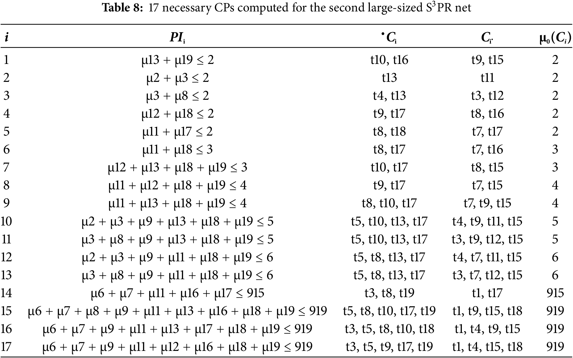
The CPNM (Nc, Mc) is constructed by merging 17 CPs with the S3PR net (N, M0) shown in Fig. 10. The CPNM is live with 59,698,137 legal markings. The permissiveness of the CPNM is 100%.

Table 9 depicts the comparison of two control policies for the second large-sized S3PR. Although the LES provided in [55] consists of only 4 CPs with weighted arcs, its behavioral permissiveness is 98,88%. On the other hand, the LES provided in Table 8 provides maximally permissive controlled behavior with 17 CPs having only ordinary arcs.

4.4 S3PGR2 Net Example

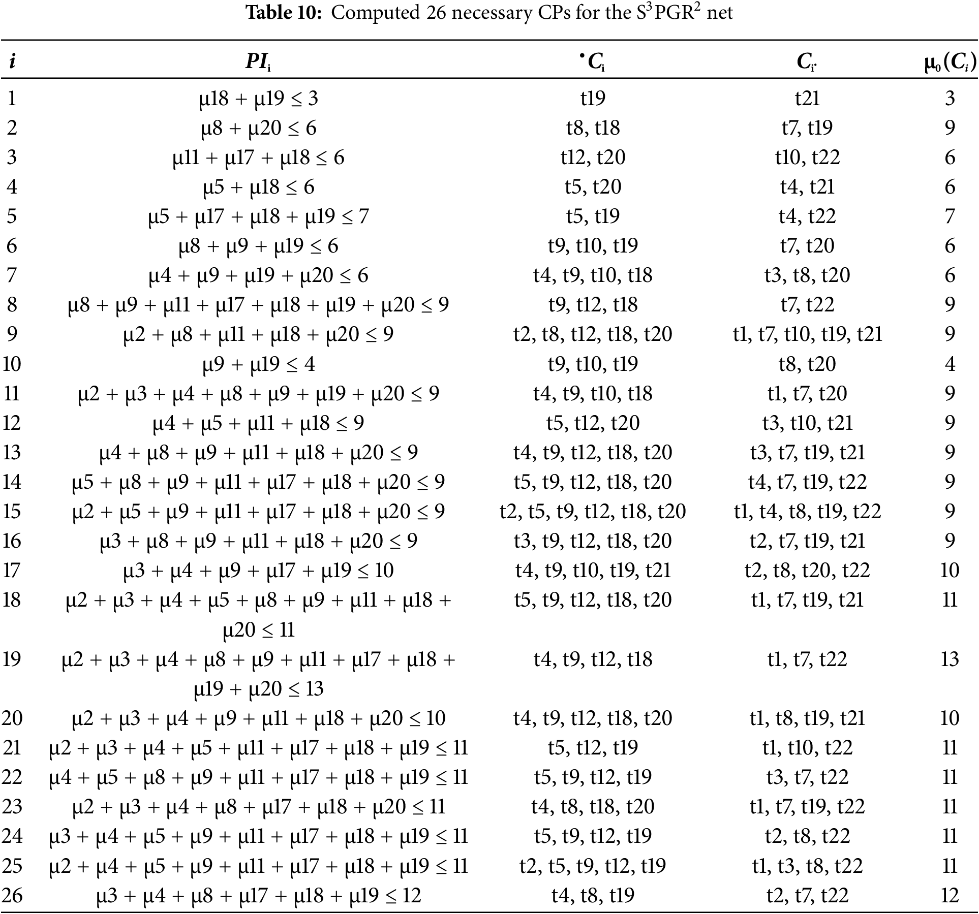
Fig. 11 shows a large-sized S3PGR2 net of an FMS with deadlock problems, which has P = {p1–p26} and T = {t1–t22} from [56]. Originally the markings of idle places p1, p7, and p16 were M(p1) = M(p7) = M(p16) = 3. The RG of this PNM has 170,312,521 markings and 1,428,308,870 transitions. The LZ and the DZ have 168,026,565 legal states and 2,285,956 illegal states, respectively. Therefore, an optimal live solution must provide 168,026,565 legal markings.

Figure 11: A large-sized S3PGR2 net from [56] with M(p1) = M(p7) = M(p16) = 50

The details of the applied procedure for this problem are omitted. By using INA, 19 SMSs of the reduced S3PGR2 net are computed. Then the complementary set of siphons [S] = {[S1], [S2], …, [S19]} are computed. Finally, by applying the proposed SbDaC policy, 19 subnets are obtained and 26 necessary CPs ψ = {C1, …, C26} with only ordinary arcs are synthesized for the S3PGR2 net as depicted in Table 10. The CPNM (Nc, Mc) is constructed by merging 26 CPs with the S3PGR2 net (N, M0) depicted in Fig. 11. The CPNM is live with 78,842,738 good markings. The permissiveness of the CPNM is 78,842,738/168,026,565 = 46.92%.

5  Conclusion

A novel siphon-based divide-and-conquer (SbDaC) policy is presented in this paper for the synthesis of PN-based LESs for FMSs suffering from deadlocks or livelocks. Given the uncontrolled and bounded PN model of an FMS with deadlock or livelock problems, a live controlled PN model of the FMS can be obtained using the SbDaC method proposed in this paper. The proposed SbDaC policy is applicable to all classes of PNs related to FMS having deadlocks or livelocks. Therefore, it is general and its use is not limited to any subclass of PNs of FMS. In theory, its off-line computation is of exponential complexity, but it is generally applicable, easy to use, effective and straightforward. The applicability and the effectiveness of the proposed method to realistic systems have been shown by considering several examples from the literature. Especially, three of these examples contain realistic FMSs with very large state spaces. In general, the method provides an optimal or a near-optimal solution in the existence of the optimal one. However, for some generalized classes of PN models of FMS, some legal states cannot be reached under the controlled behavior, resulting in less permissive behavior. Therefore, further research is necessary to provide new policies to achieve more permissive LESs for generalized classes of PNs. It is also necessary to carry out further research to reduce the structural complexity of the computed LESs.

Acknowledgement: The authors extend their appreciation to King Saud University, Saudi Arabia for funding this work through the Ongoing Research Funding Program (ORF-2025-704), King Saud University, Riyadh, Saudi Arabia.

Funding Statement: The authors extend their appreciation to King Saud University, Saudi Arabia for funding this work through the Ongoing Research Funding Program (ORF-2025-704), King Saud University, Riyadh, Saudi Arabia.

Author Contributions: The authors confirm contribution to the paper as follows: Conceptualization: Murat Uzam, Wei Wei, Yufeng Chen; methodology: Murat Uzam, Wei Wei, Yufeng Chen, Mohammed El-Meligy; software: Bernard Berthomieu, Wei Wei, Yufeng Chen, Mohamed Abdel Fattah Sharaf; validation: Bernard Berthomieu, Mohammed El-Meligy, Mohamed Abdel Fattah Sharaf; formal analysis: Murat Uzam, Wei Wei, Yufeng Chen, Mohammed El-Meligy; analysis and interpretation of results: Murat Uzam, Bernard Berthomieu, Yufeng Chen; draft manuscript preparation: Murat Uzam, Bernard Berthomieu, Yufeng Chen, Mohamed Abdel Fattah Sharaf; review and editing: Bernard Berthomieu, Mohammed El-Meligy, Mohamed Abdel Fattah Sharaf; funding acquisition: Mohammed El-Meligy, Mohamed Abdel Fattah Sharaf. All authors reviewed the results and approved the final version of the manuscript.

Availability of Data and Materials: Petri net definitions of the example Petri nets utilized in this article are provided for the analysis of these nets by using INA and/or TINA Petri net tools.

Ethics Approval: Not applicable.

Conflicts of Interest: The authors declare no conflicts of interest to report regarding the present study.

References

1. Li Z, Zhou M. Deadlock resolution in automated manufacturing systems: a novel petri net approach. Berlin/Heidelberg, Germany: Springer; 2009. doi:10.1007/978-1-84882-244-3. [Google Scholar] [CrossRef]

2. David R, Alla H. Discrete, continuous, and hybrid petri nets. Berlin/Heidelberg, Germany: Springer; 2005. doi:10.1007/978-3-642-10669-9. [Google Scholar] [CrossRef]

3. Wu NQ, Zhou MC, Li ZW. Short-term scheduling of crude-oil operations: enhancement of crude-oil operations scheduling using a Petri net-based control-theoretic approach. IEEE Robot Autom Mag. 2015;22(2):64–76. doi:10.1109/MRA.2015.2417651. [Google Scholar] [CrossRef]

4. Xing K, Hu B, Chen H. Deadlock avoidance policy for flexible manufacturing systems. In: Zhou MC, editor. Petri nets in flexible and agile automation. Boston, MA, USA: Kluwer; 1995. p. 239–63. doi:10.1007/978-1-4615-2231-7_9. [Google Scholar] [CrossRef]

5. Xing K, Hu B, Chen H. Deadlock avoidance policy for Petri-net modeling of flexible manufacturing systems with shared resources. IEEE Trans Autom Control. 1996;41(2):289–95. doi:10.1109/9.481517. [Google Scholar] [CrossRef]

6. Yang Y, Liu Z, Zhao Z, Zhou M. Deadlock analysis and avoidance for automated manufacturing systems based on petri nets with forward-conflict-free structures. IEEE Trans Syst Man Cybern Syst. 2025;55(3):1634–46. doi:10.1109/TSMC.2024.3509901. [Google Scholar] [CrossRef]

7. Capkovic F. Modelling and control of resource allocation systems within discrete event systems by means of Petri nets—part 1: invariants, siphons and traps in deadlock avoidance. Comput Inform. 2021;40(3):648–89. doi:10.31577/cai_2021_3_648. [Google Scholar] [CrossRef]

8. Yang B, Hu H. Maximally permissive deadlock and livelock avoidance for automated manufacturing systems via critical distance. IEEE Trans Autom Sci Eng. 2022;19(4):3838–52. doi:10.1109/TASE.2021.3138169. [Google Scholar] [CrossRef]

9. Tat Leung Y, Sheen G-J. Resolving deadlocks in flexible manufacturing cells. J Manuf Syst. 1993;12(4):291–304. doi:10.1016/0278-6125(93)90320-S. [Google Scholar] [CrossRef]

10. Cho H, Kumaran TK, Wysk RA. Graph-theoretic deadlock detection and resolution for flexible manufacturing systems. IEEE Trans Robot Autom. 1995;11(3):413–21. doi:10.1109/70.388784. [Google Scholar] [CrossRef]

11. Pan YL, Tseng CY, Chen JC. Enhancement of computational efficiency for deadlock recovery of flexible manufacturing systems using improved generating and comparing aiding matrix algorithms. Processes. 2023;11(10):3026. doi:10.3390/pr11103026. [Google Scholar] [CrossRef]

12. Ezpeleta J, Colom JM, Martinez J. A Petri net based deadlock prevention policy for flexible manufacturing systems. IEEE Trans Robot Autom. 1995;11(2):173–84. doi:10.1109/70.370500. [Google Scholar] [CrossRef]

13. Uzam M. An optimal deadlock prevention policy for flexible manufacturing systems using Petri net models with resources and the theory of regions. Int J Adv Manuf Technol. 2002;19(3):192–208. doi:10.1007/s001700200014. [Google Scholar] [CrossRef]

14. Wang S, Guo X, Karoui O, Zhou M, You D, Abusorrah A. A refined siphon-based deadlock prevention policy for a class of Petri nets. IEEE Trans Syst Man Cybern Syst. 2023;53(1):191–203. doi:10.1109/TSMC.2022.3174421. [Google Scholar] [CrossRef]

15. Li C, Jin F, Chen Y, Li Z, Uzam M, Ma H. Calculation and analysis of Petri net reachability graphs by a think-globally-act locally method. Mathematics. 2025;13(5):793. doi:10.3390/math13050793. [Google Scholar] [CrossRef]

16. Capkovic F. Petri net-based S3PR models of automated manufacturing systems with resources and their deadlock prevention. Acta Polytech Hung. 2023;20(6):79–96. [Google Scholar]

17. Row T, Pan Y. Incomparable single controller for solving deadlock problems of flexible manufacturing systems. IEEE Access. 2023;11:45270–8. doi:10.1109/ACCESS.2023.3272227. [Google Scholar] [CrossRef]

18. Yang Y, Yang J, Liang N, Zhong C. Control law for two-process flexible manufacturing systems modeled using petri nets. Mathematics. 2025;13(4):611. doi:10.3390/math13040611. [Google Scholar] [CrossRef]

19. Ma T, Wang J, Hu H. A strict minimal siphon-based necessary and sufficient condition for liveness verification in general petri nets. IEEE Access. 2025;13:53517–30. doi:10.1109/ACCESS.2025.3551396. [Google Scholar] [CrossRef]

20. Yang B, Hu H. On the equivalence between robustness and liveness in automated manufacturing systems. IEEE Trans Syst Man Cybern Syst. 2024;54(12):7495–507. doi:10.1109/TSMC.2024.3458939. [Google Scholar] [CrossRef]

21. Fan X, Hu H, Yang B, Liu Y, He G. Event circuit structures for deadlock avoidance in flexible manufacturing systems. IEEE Trans Autom Sci Eng. 2023;20(1):597–610. doi:10.1109/TASE.2022.3163854. [Google Scholar] [CrossRef]

22. Huang YS, Jeng MD, Xie X, Chung DH. Siphon-based deadlock prevention policy for flexible manufacturing systems. IEEE Trans Syst Man Cybern Part A Syst Hum. 2006;36(6):1248–56. doi:10.1109/TSMCA.2006.878953. [Google Scholar] [CrossRef]

23. Piroddi L, Cordone R, Fumagalli I. Combined siphon and marking generation for deadlock prevention in Petri nets. IEEE Trans Syst Man Cybern Part A Syst Hum. 2009;39(3):650–61. doi:10.1109/TSMCA.2009.2013189. [Google Scholar] [CrossRef]

24. Hou Y, Li ZW, Zhao M, Liu D. Extended elementary siphon-based deadlock prevention policy for a class of generalised Petri nets. Int J Comput Integr Manuf. 2014;21(1):85–102. doi:10.1080/0951192X.2013.800233. [Google Scholar] [CrossRef]

25. Hou Y, Zhao M, Liu D, Hong L. An efficient siphon-based deadlock prevention policy for a class of generalized Petri nets. Discret Dyn Nat Soc. 2016;2016:8219424. doi:10.1155/2016/8219424. [Google Scholar] [CrossRef]

26. Uzam M, Zhou MC. An iterative synthesis approach to Petri net-based deadlock prevention policy for flexible manufacturing systems. IEEE Trans Syst Man Cybern Part A Syst Hum. 2007;37(3):362–71. doi:10.1109/TSMCA.2007.893484. [Google Scholar] [CrossRef]

27. Chen YF, Li ZW, Khalgui M, Mosbahi O. Design of a maximally permissive liveness-enforcing Petri net supervisor for flexible manufacturing systems. IEEE Trans Autom Sci Eng. 2010;8(2):374–93. doi:10.1109/TASE.2010.2060332. [Google Scholar] [CrossRef]

28. Xing K, Zhou M, Wang F, Liu H, Tian F. Resource-transition circuits and siphons for deadlock control of automated manufacturing systems. IEEE Trans Syst Man Cybern Part A Syst Hum. 2011;41(1):74–84. doi:10.1109/TSMCA.2010.2048898A. [Google Scholar] [CrossRef]

29. Capkovic F. Control of deadlocked discrete-event systems using petri nets. Acta Polytech Hung. 2022;19(2):213–33. [Google Scholar]

30. Al-Shayea A, Kaid H, Al-Ahmari A, Nasr EA, Kamrani AK, Mahmoud HA. Colored resource-oriented petri nets for deadlock control and reliability design of automated manufacturing systems. IEEE Access. 2021;9:125616–27. doi:10.1109/ACCESS.2021.3111575. [Google Scholar] [CrossRef]

31. Bashir M, Zhou J, Muhammad BB. Optimal supervisory control for flexible manufacturing systems model with petri nets: a place-transition control. IEEE Access. 2021;9:58566–78. doi:10.1109/ACCESS.2021.3072892. [Google Scholar] [CrossRef]

32. Tseng C, Chen J, Pan Y. An improved deadlock recovery policy of flexible manufacturing systems based on resource flow graphs. IEEE Access. 2024;12(3):65202–12. doi:10.1109/ACCESS.2024.3396879. [Google Scholar] [CrossRef]

33. Dou H, Zhou M, Wang S, Albeshri A. An efficient liveness analysis method for petri nets via maximally good-step graphs. IEEE Trans Syst Man Cybern Syst. 2024;54(7):3908–19. doi:10.1109/TSMC.2024.3372941. [Google Scholar] [CrossRef]

34. Feng Y, Ren S, Cao Y, Xing K, Yang Y. Deadlock control for flexible assembly systems with multiple resource requirements and separately-loaded parts. IEEE Trans Autom Sci Eng. 2025;22(2):9275–84. doi:10.1109/TASE.2024.3504714. [Google Scholar] [CrossRef]

35. Li Y, Chen Y, Zhou R. A set covering approach to design maximally permissive supervisors for flexible manufacturing systems. Mathematics. 2024;12(11):1687. doi:10.3390/math12111687. [Google Scholar] [CrossRef]

36. Uzam M, El-Sherbeeny AM, Guo W, Li ZW. Design of an improved think globally act locally approach for the computation of Petri nets based liveness-enforcing supervisors of FMSs. IEEE Access. 2024;12(4):74367–88. doi:10.1109/ACCESS.2024.3403804. [Google Scholar] [CrossRef]

37. Li Z, Zhu S, Zhou M. A Divide-and-conquer strategy to deadlock prevention in flexible manufacturing systems. IEEE Trans Syst Man Cybern. 2009;39(2):156–69. doi:10.1109/TSMCC.2008.2007246. [Google Scholar] [CrossRef]

38. Uzam M, Li Z, Gelen G, Zakariyya R. A divide-and-conquer-method for the synthesis of liveness-enforcing supervisors for flexible manufacturing systems. J Intell Manuf. 2016;27(5):1111–29. doi:10.1007/s10845-014-0938-z. [Google Scholar] [CrossRef]

39. Zhong C, He W, Li Z, Wu N, Qu T. Deadlock analysis and control using Petri net decomposition techniques. Inf Sci. 2019;482(6):440–56. doi:10.1016/j.ins.2019.01.029. [Google Scholar] [CrossRef]

40. Uzam M, Zhou MC. An improved iterative synthesis method for liveness-enforcing supervisors of flexible manufacturing systems. Int J Prod Res. 2006;44(10):1987–2030. doi:10.1080/00207540500431321. [Google Scholar] [CrossRef]

41. INA Integrated Net Analyzer, a software tool for analysis of PNs, Version 2.2 [Internet]. 2022 [cited 2025 Jul 29]. Available from: http://www.informatik.hu-berlin.de/~starke/ina.html. [Google Scholar]

42. TINA. Time petri net analyzer [Internet]. [cited 2025 Jul 29]. Available from: https://projects.laas.fr/tina/index.php. [Google Scholar]

43. Uzam M, Liu D, Berthomieu B, Gelen G, Zhang Z, Mostafa AM, et al. On deadlock/livelock studies based on reachability graph of Petri nets by using TINA. IEEE Access. 2024;12(3):135506–34. doi:10.1109/ACCESS.2024.3461168. [Google Scholar] [CrossRef]

44. Liu G, Barkaoui K. A survey of siphons in Petri nets. Inf Sci. 2016;363:198–220. doi:10.1016/j.ins.2016.02.010. [Google Scholar] [CrossRef]

45. Li ZW, Zhou M. Elementary siphons of Petri nets and their application to deadlock prevention in flexible manufacturing systems. IEEE Trans Syst Man Cybern Part A Syst Hum. 2004;34(1):38–51. doi:10.1109/TSMCA.2003.820576. [Google Scholar] [CrossRef]

46. Chen YF, Li ZW, Al-Ahmari A. Nonpure Petri net supervisors for optimal deadlock control of flexible manufacturing systems. IEEE Trans Syst Man Cybern Part A Syst Hum. 2013;43(2):252–65. doi:10.1109/TSMCA.2012.2202108. [Google Scholar] [CrossRef]

47. Yamalidou K, Moody J, Lemmon M, Antsaklis P. Feedback control of Petri nets based on place invariants. Automatica. 1996;32(1):15–28. doi:10.1016/0005-1098(95)00103-4. [Google Scholar] [CrossRef]

48. Uzam M, Li Z, Zhou M. Identification and elimination of redundant control places in Petri net based liveness-enforcing supervisors of FMS. Int J Adv Manuf Technol. 2007;35(1–2):150–68. doi:10.1007/s00170-006-0701-5. [Google Scholar] [CrossRef]

49. Heiner M, Schwarick M, Wegener JT. Charlie—an extensible petri net analysis tool. In: Devillers R, Valmari A, editors. In:Application and theory of petri nets and concurrency. Vol. 9115. Cham, Switzerland: Springer; 2015. doi:10.1007/978-3-319-19488-2_10. [Google Scholar] [CrossRef]

50. Liu F, Assaf G, Chen M, Heiner M. A Petri nets-based framework for whole-cell modeling. Biosystems. 2021;210(0237):104533. doi:10.1016/j.biosystems.2021.104533. [Google Scholar] [PubMed] [CrossRef]

51. Yan M, Li Z, Wei N, Zhao M. A deadlock prevention policy for a class of Petri nets S3PMR*. J Inf Sci Eng. 2009;25(1):167–83. doi:10.6688/JISE.2009.25.1.9. [Google Scholar] [CrossRef]

52. Feng Y, Ren S, Ren X, Chen H, Yang Y. Small-size liveness-enforcing supervisor for automated manufacturing systems using the theory of transition cover. IEEE Trans Syst Man Cybern Syst. 2023;53(4):2222–35. doi:10.1109/TSMC.2022.3209156. [Google Scholar] [CrossRef]

53. Row T, Tseng C, Pan Y. Universal single controller for solving deadlock problems of flexible manufacturing systems. IEEE Access. 2024;12(12):191907–20. doi:10.1109/ACCESS.2024.3515462. [Google Scholar] [CrossRef]

54. Li Z, Zhou M. Comparison of two deadlock prevention methods for different-size flexible manufacturing systems. Int J Intell Control Syst. 2005;10(3):235–43. [Google Scholar]

55. Dou H, You D, Wang S, Zhou M. Designing liveness-enforcing supervisors for manufacturing systems by using maximally good step graphs of petri nets. IEEE Trans Autom Sci Eng. 2025;22:7312–23. doi:10.1109/TASE.2024.3450656. [Google Scholar] [CrossRef]

56. Hu H, Li Z. Local and global deadlock prevention policies for resource allocation systems using partially generated reachability graphs. Comput Ind Eng. 2009;57(4):1168–81. doi:10.1016/j.cie.2009.05.006. [Google Scholar] [CrossRef]