An Optimized Customer Churn Prediction Approach Based on Regularized Bidirectional Long Short-Term Memory Model

1  Introduction

Customer churn prediction is a crucial challenge for organizations, particularly in sectors such as telecommunications, banking, and e-commerce, as retaining customers is less expensive than acquiring new ones [1]. Churn occurs when customers cease using a product or service, resulting in revenue loss. Accurate churn prediction enables businesses to implement proactive retention initiatives, such as targeted offers and enhanced customer service [2]. Customer churn is a significant threat to profitability and market share, as it is the process that causes consumers to discontinue using a company’s services and switch to a competitor [3]. Numerous causes, including dissatisfaction with pricing, customer service, or service quality, as well as the availability of superior offers from competitors, can lead to customer turnover. Market positioning and brand reputation are also impacted by churn, in addition to the loss of revenue. To proactively retain consumers and enhance overall business performance, telecom businesses have made it a top priority to understand and predict customer churn [4,5]. According to [6], keeping clients can therefore result in significant cost savings and increased profitability.

Furthermore, companies in the telecom industry are now compelled to concentrate more on customer-centric strategies due to regulatory restrictions and heightened competition [7]. Because governments and regulatory agencies frequently enforce stringent limitations on pricing and service quality, telecom businesses must constantly exceed customer expectations. Penalties, legal challenges, and further loss of customers to competitors may arise from failure to comply. In this context, effective customer retention strategies are essential for maintaining a competitive edge and ensuring long-term business success [8].

Churn prediction models are widely utilized across various sectors. Companies in the telecommunications sector utilize churn prediction to identify high-risk consumers and provide targeted retention incentives [9]. Banks use churn models to monitor transaction behaviors and consumer engagement patterns, allowing them to create tailored loyalty programs [10,11]. E-commerce behemoths such as Amazon and Netflix utilize predictive analytics to enhance customer experiences and decrease subscription cancellations by offering personalized recommendations [9]. As the volume and complexity of customer data increase, organizations are investing more in artificial intelligence and deep learning models to enhance their churn prediction capabilities. Churn prediction methods have evolved, moving from traditional statistical models to more advanced machine learning and deep learning approaches. However, these complex models have higher computing costs and require large datasets for practical training.

The goal of this work is to enhance the accuracy and interpretability of customer churn prediction by leveraging a Bidirectional LSTM model with regularization. Additionally, this study aims to expand the body of knowledge on customer churn prediction by developing an enhanced RBiLSTM-based model that incorporates dropout, early stopping, and regularization techniques to improve generalization and performance. Furthermore, the study examines the impact of various optimization algorithms, including Adaptive Moment Estimation (Adam), Stochastic Gradient Descent (SGD), and Root Mean Squared Propagation (RMSprop), on model convergence and accuracy in business decision-making. The remainder of this paper is structured as follows: Section 2 provides a comprehensive literature review of traditional and deep learning-based churn prediction approaches. Section 3 details the proposed approach and its stages. Section 4 presents the hypotheses and experimental design, and Section 5 provides the conclusion, along with future research directions.

2  Literature Review

Customer churn prediction has been a topic of considerable research interest for decades due to its significant impact on business profitability and sustainability. Researchers have employed a range of approaches, from traditional statistical models to advanced machine learning and deep learning techniques. This section provides an in-depth overview of the existing literature on customer churn prediction, categorizing approaches into traditional methods, machine learning techniques, and deep learning enhancements. A one-size-fits-all strategy to retention fails to address the unique demands and preferences of distinct consumer categories, resulting in poor performance [12,13]. Machine learning represents a substantial improvement over traditional methods for attrition prediction and customer retention in the telecom industry. Unlike conventional models, which frequently rely on predefined rules and linear correlations, machine learning models can learn from data and adapt to new information, making them more adaptable and accurate [14–16].

A number of machine learning approaches based on supervised, unsupervised, and ensemble methods have been widely used in churn prediction. Early studies on customer churn relied heavily on supervised learning methods, such as Logistic Regression (LR), Decision Trees (DT), Naïve Bayes (NB), Support Vector Machines (SVM), K-Nearest Neighbors (KNN), Gradient Boosting (GB), and Adaptive Boosting (AdaBoost) [17]. These models provide interpretable results and are commonly used in industries such as telecommunications and banking [18]. Similarly, in the research of [19], LR and DT are used to predict customer churn. Their results showed that DT outperformed LR in their datasets. They obtained the highest accuracy of 99.67% on their large dataset using DT. Ensemble approaches, which combine multiple models to enhance prediction performance, are gaining popularity in churn prediction.

For example, the RF method is used to enhance prediction accuracy and identify complex relationships between variables that indicate churn risk [20]. Additionally, KNN, RF, and Extreme Gradient Boosting (XGBoost) are employed by [21] to predict customer churn. In their research, XGBoost achieved the highest accuracy of 79.8% and the highest Area Under the Curve (AUC) of 58.2%. Moreover, KNN, NB, DT, RF, AdaBoost, and ANN are also used by [22] to predict customer turnover. They used the Synthetic Minority Over-sampling Technique (SMOTE) to balance the instances in their dataset. Different parameter combinations of various algorithms are explored to obtain the most adequate model. In their research, the KNN, DT, and RF classifiers performed well in terms of AUC value. The results also showed that RF ranked top, at 91.10%. Methods such as bagging and boosting combine the predictions of multiple base models to reduce volatility and bias, resulting in more robust and accurate results. These models are especially beneficial when dealing with noisy data or complex variable relationships [23]. In the research of [24], the performance of more than 100 classifiers was compared in the context of churn prediction in the telecom industry. Their results showed that regularized RF achieved the highest accuracy of 73.04%, while bagging RF outperformed all other classifiers in terms of AUC, with a score of 67.20%. Imani and Arabnia [25] presented a work on churn prediction using a number of classifiers, including Categorical Boosting (CatBoost), optimized CatBoost, Light Gradient Boosting Machine (LightGBM), optimized LightGBM, XGBoost, and optimized XGBoost. They achieved 90%, 93%, 91%, 90%, 90%, and 91% of F1-score, respectively. Idris et al. [26] investigated under-sampling methods based on particle swarm optimization (PSO) with various feature reduction methods, utilizing random forest and KNN classifiers. Experimental results showed that the method based on PSO performed the best in terms of AUC, at 75.11%.

Another trend is the hybrid model, which combines classic statistical approaches with machine learning techniques. These models combine the best features of both approaches, use machine learning to capture non-linear patterns while maintaining the interpretability and simplicity of older methods. For example, a hybrid model employs the LR for ease of understanding and the neural network (NN) to capture intricate interactions between variables [27]. Clustering and principal component analysis (PCA) are unsupervised learning approaches that divide clients into groups based on similar features or behaviors. These strategies do not require labeled data and are beneficial for identifying hidden patterns or consumer segments that are at risk of churn. Clustering, for example, can categorize customers based on their usage patterns, allowing telecom businesses to adapt retention efforts to specific segments [28].

Although these traditional models are effective in handling structured tabular data, they struggle with complex, high-dimensional datasets where relationships between variables are non-linear. Another challenge with traditional models is the manual feature selection required to improve accuracy. In industries, the behavior of customers is highly dynamic, and static models similar to LR are insufficient. This limitation led to the adoption of machine learning models that could automatically learn patterns from large-scale customer data. Recent machine learning research on churn prediction has focused on enhancing model accuracy, interpretability, and scalability. One significant trend is the incorporation of deep learning techniques, such as neural networks, which can model complex, non-linear relationships and analyze unstructured data, including text and images. For example, recurrent neural networks (RNNs) have been utilized to improve attrition forecasting by analyzing sequential customer data, such as call logs or browser histories [29].

Recent studies have highlighted the significant advancements in deep learning architectures and meta-modeling methods for customer churn prediction. To enhance early churn identification in large-scale systems, Bhattacharjee et al. [30] developed a multivariate time series classification method that utilizes historical user–product interactions. On the other hand, Multilayer Perceptron (MLP) [17], Convolutional Neural Network (CNN), Feedforward Neural Network (FNN), and Recurrent Neural Networks (RNNs)-based models, along with their variations such as Long Short-Term Memory (LSTM) [31,32], Gated Recurrent Unit (GRU), Bidirectional Long Short-Term Memory Network (BiLSTM), and ensemble (LSTM+GRU) [32] have demonstrated better performance when processing behavioral and sequential data. To improve accuracy and interpretability, Rudd et al. [33] introduced a multimodal fusion model in the financial services industry that combines behavioral signals, speech data, and client financial literacy.

A more recent method by Bai et al. [34] demonstrated that deep sequential models remain highly successful for RFM-based churn prediction, indicating that classic RNNs outperform transformers when modeling time-variable parameters. Asfe et al. [35] integrated a Tabular Neural Network (TabNet) transformer with meta-model integration to build ensemble neural architectures and feature selection through Neighborhood Component Analysis (NCA) in the context of e-commerce. Customer churn prediction has advanced significantly in recent years, especially with the combination of explainable AI and deep learning techniques. Asif et al. [36] proposed an explainable and interpretable model for telecom customer churn prediction to ensure model transparency, trust, and improve decision-making. Moreover, the churn prediction task is enhanced by the clever deep fusion of attention-based models that emphasize attention processes, hybrid and ensemble techniques, and the timeless value of sequence modeling to complement and validate the decisions made in the financial services domain [37].

Finally, Ahmed et al. [38] used a deep learning method and proposed a technique called ‘TL-DeepE’, which first conducted Transfer Learning (TL) by fine-tuning multiple pre-trained deep convolutional neural networks (CNNs). They converted the telecom dataset into a 2D image format. Then, they used these CNNs as base classifiers, and Genetic Programming (GP) and AdaBoost as the meta-classifier. Their method obtained an accuracy of 75.4% and 68.2%, and an AUC of 83% and 74%, for the Orange and Cell2Cell datasets, respectively.

In short, approaches to customer churn prediction have developed several models, extending from traditional statistical-based models to advanced deep learning-based models. Although LR and DTs are early solutions, they have limitations in dealing with complicated, high-dimensional data. Other learning algorithms, such as RF, GB, and SVM, have improved the accuracy of churn prediction but remain ineffective with sequential data. However, deep learning, particularly BiLSTM and transformers with regularization, can enhance companies’ ability to collect temporal client behavior and address issues related to class imbalance, overfitting, and generalization error.

3  Proposed Approach

This study develops a robust and systematic approach for customer churn prediction using a Regularized Bidirectional Long Short-Term Memory (RBiLSTM) model. The approach consists of seven well-defined stages, which are benchmark dataset description, data preprocessing and splitting, model architecture, hyper-parameter optimization, model training and evaluation, and model comparison with Long-Short Term Memory (LSTM), Deep Neural Network (DNN), and other traditional classifiers, such as Logistic Regression (LR), Decision Tree (DT), K-Nearest Neighbors (KNN), and Support Vector Machine (SVM). In Fig. 1, the main stages of the proposed approach are illustrated, and the following subsections provide detailed explanations and descriptions of its stages.

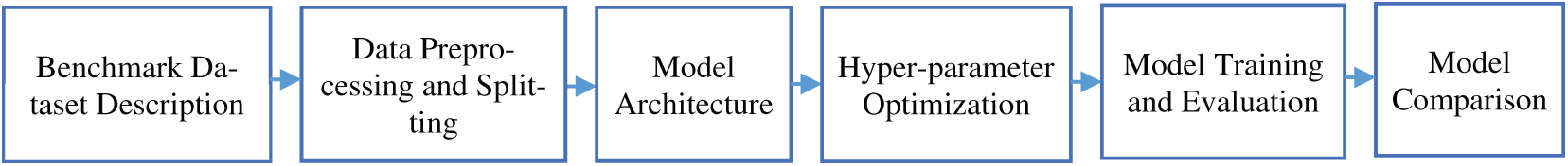
Figure 1: Flowchart of the proposed approach

3.1 Benchmark Dataset Description

The labeled Customer Churn Prediction 2020 dataset [39] is used in this study, which contains comprehensive customer-related information collected from a telecommunications service provider. It consists of 4250 instances with 20 features, including the target variable. The target variable, churn, is a categorical variable with a yes/no value, indicating whether the customer left the service (yes) or stayed (no). Table 1 provides a detailed description of each feature, including its data type and a brief explanation. The dataset captures customer demographics, service usage, and churn behavior. The number of instances based on the classes and their distributions are shown in Fig. 2.

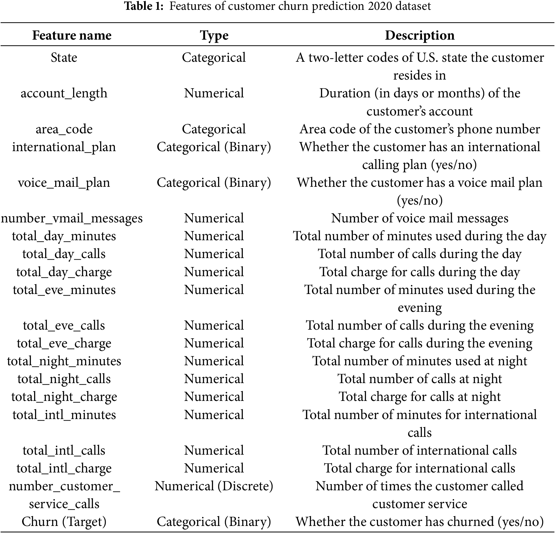
Figure 2: Number of instances based on the classes and their distribution

3.2 Data Preprocessing and Splitting

Before model training, comprehensive data preprocessing is essential to ensure the dataset is clean, consistent, and suitable for input into the neural network. Missing values are handled using appropriate strategies such as imputation with the mean for numerical and with the mode for categorical features. Features of binary categorical values, such as international plan and voicemail plan, are transformed using one-hot encoding to convert them into a numerical format. Other numerical features are scaled using Z-score normalization to bring them into a similar range, thereby improving model convergence. The Z-score normalization is defined in [40] using Eq. (1):

z=x−μσ,(1)

where z is the new scaled value (standardized), x is the original value, μ is the mean of the feature, and σ is the standard deviation of the feature.

Additionally, the usefulness of categorical features such as state and area_code is removed because encoding them introduces many additional dimensions, which can cause overfitting, especially with small datasets, and lead to sparsity in the feature matrix, as well as increase model complexity. Following preprocessing, the dataset is split into training, validation, and test sets using stratified sampling with a 70:10:20 ratio, thereby maintaining the class distribution throughout the splitting process. The validation set is used during model training to monitor overfitting and fine-tune model parameters.

3.3 Model Architecture

This study is based on an RBiLSTM network design. The RBiLSTM captures past and future context concurrently by processing input sequences in both forward and backward orientations, in contrast to typical LSTM models. In customer churn situations, this is especially helpful because customer behavior over time, such as the number of customer service calls, an increase in support calls, or payment changes, can provide informative data features. The model architecture consists of two BiLSTM layers, followed by a dense input layer. The dense input layer is fully connected and can accept the values of the input features, which are primarily tabular and non-sequential. Dropout layers, which randomly deactivate neurons during training, are designed to reduce overfitting. For binary classification, a last dense layer with a sigmoid activation function is used. Additionally, L2-regularization with early stopping techniques is employed to prevent overfitting and ensure improved generalization. Fig. 3 presents the flowchart structure of the developed model that consists of the following components:

1.    Input Layer: It contains several units that match the total number of input features after preprocessing (17 features), with a ReLU activation function to introduce non-linearity.

2.    Bidirectional LSTM (64 units) with L2-regularization: It captures dependencies in both forward and backward directions.

3.    Dropout (0.2): It randomly deactivates 20% of neurons to reduce overfitting.

4.    Bidirectional LSTM (32 units) with L2-regularization: It captures further temporal dependencies and higher-level patterns.

5.    Dropout (0.2): It randomly deactivates 20% of neurons as an additional regularization technique to reduce overfitting and prevent the co-adaptation of neurons.

6.    Dense Layer (1 unit, Sigmoid Activation): It outputs a probability between 0 and 1, indicating the likelihood of churn.

Figure 3: Flowchart structure of the developed RBiLSTM model

Based on deep learning best practices, the RBiLSTM model consists of two BLSTM (64 units) and one BLSTM (32 units) with L2 Regularization and two dropout layers, each with a dropout rate of 0.2 and L2 Regularization. The dropout rate of 0.2 is selected because lower values have a minimal influence on overfitting, while rates greater than 0.2 result in underfitting. Therefore, the trade-off value between regularization and model capacity is offered by the 0.2 rate. Similarly, the L2-regularization parameter is chosen to be 0.001, which represents the trade-off value for penalizing large weights while reducing model complexity without affecting convergence. With the validation loss as the monitored parameter, early stopping is used to avoid the overfitting problem further. If the validation loss did not decrease for five consecutive epochs (patience = 5), the training procedure was terminated. This early stopping criterion increased generalization on the unseen test set by guaranteeing effective training while maintaining the top-performing model weights. After building the model architecture, it is compiled by defining the optimization algorithm with its default hyperparameter values, a binary cross-entropy loss function, an early stopping technique, and a loss value as the validation metric.

3.4 Hyper-Parameter Optimization

Hyper-parameter optimization plays a crucial role in improving the performance of the developed model. In this study, several hyper-parameters are fine-tuned, including the batch size, learning rate, number of epochs, and the optimizer methods. A range of batch sizes, including (16, 32, 64, and 128) is tested to find the optimal trade-off between speed and training stability. Different optimization methods, such as Adaptive Moment Estimation (Adam), Stochastic Gradient Descent (SGD), and Root Mean Squared Propagation (RMSprop), are evaluated to determine which one provides the best generalization and fastest convergence. A combination of manual tuning and grid search is employed to determine the optimal values, while early stopping and learning rate scheduling are implemented to prevent overfitting and reduce training time. The binary cross-entropy loss function is used due to the binary nature of the target variable. Algorithm 1 gives the pseudocode of hyper-parameter optimization.

The best values of hyper-parameters in the optimization stage are used to train the model, ensuring an optimal balance between convergence speed, generalization, and accuracy.

3.5 Model Training and Evaluation

The model is trained using the training set, and the performance is evaluated on a hold-out test set. After training the model, the hold-out validation set is used to ensure that the results are generalized, thereby avoiding dependency on a particular train-test split. Confusion matrices are analyzed to understand the distribution of true positives (TP), true negatives (TN), false positives (FP), and false negatives (FN), offering insights into the types of errors the model was making. The training and validation curves are plotted to visualize the model’s discriminative power. Several evaluation metrics are used to assess the effectiveness of the RBiLSTM model, including accuracy, Precision, Recall, F1-score, and the Receiver Operating Characteristic (ROC) curve. The standard definitions of these metrics are described in [41], chosen to provide a fair view of the models’ performance, and computed using Eqs. (2)–(5):

Accuracy=(TP+ TN)(TP+TN+FP+FN)(2)

Recall=TP(TP+FN)(3)

Precision=TP(TP+FP)(4)

F1−score=2∗(Precision * Recall)(Precision + Recall)(5)

3.6 Model Comparison

The model comparison stage is a crucial part of validating the effectiveness of the proposed RBiLSTM model. The goal of this stage is to perform a benchmark performance of RBiLSTM against traditional ML and deep learning models. This study is conducted using several baseline machine learning models, including Logistic Regression (LR), Decision Tree (DT), K-Nearest Neighbors (KNN), Support Vector Machine (SVM), a standard Deep Neural Network (DNN), and an LSTM model. Each baseline is trained on the same preprocessed dataset and evaluated using consistent metrics for fair comparison. This comparative analysis enables us to determine whether the complexity and temporal awareness of the RBiLSTM model truly yield a measurable performance improvement. Additionally, it allows us to position the proposed RBiLSTM model in relation to simpler and widely used alternatives, highlighting its strengths in capturing sequential dependencies and enhancing predictive performance. Algorithm 2 summarizes the model comparison for churn prediction.

4  Hypotheses and Experimental Design

This section begins by familiarizing readers with a number of research questions that form the foundation of the experimental design and evaluation. Then, the Section 4.1 clarifies the steps of the procedure solution, showing the order of equations presented in the Section 3. After that, the Section 4.2 presents the experimental results with a detailed discussion for each step of the experimental procedure. As mentioned earlier in the introduction, the main goal of this study is to develop RBiLSTM and build an accurate and comprehensible model for customer churn prediction. In order to ensure feasibility, fairness, interpretability, this work also attempts to compare the performance of the proposed model to conventional ML, DNN classifiers, and typical LSTM architectures. For the direction of this investigation, the following research questions are described as hypotheses:

RQ1: The optimized BiLSTM model outperforms LSTM, DNN, and traditional ML classifiers, such as LR, DT, KNN, and SVM, in terms of classification accuracy and F1-score.

RQ2: The use of 10-fold cross-validation validates the model performance and provides a reliable estimate of the used train-test split.

RQ3: The performance results of the RBiLSTM model using SMOTE on the training set are lower than the results without using the SMOTE method.

RQ4: The inclusion of regularization, early stopping, and the hyper-parameter tuning process reduces overfitting and enhances the generalization ability of the BiLSTM model.

RQ5: Model explainability using SHAP provides transparent insights into individual predictions.

4.1 Experimental Procedure

In this subsection, the steps of the experimental procedure, which implements the research approach, are described to create, train, and test the RBiLSTM model for customer churn prediction. The steps begin with data preprocessing, which includes removing unnecessary features and normalizing them with Z-score standardization. To maintain class distribution, the dataset is divided into training, validation, and test sets in a 70:10:20 ratio. To ensure robust performance, baseline models including LR, DT, KNN, SVM, DNN, and standard LSTM are used for comparison. Grid search and early stopping methods are used to tune hyperparameters. Models are evaluated using standard metrics, such as accuracy, precision, recall, and F1-score, followed by an explainability analysis using SHAP to understand the predictions. This experimental workflow guarantees a thorough and interpretable examination of the developed model. Algorithm 3 outlines the steps of the experimental procedure, presenting the equations of the proposed solution in order.

4.2 Evaluation Results and Discussions

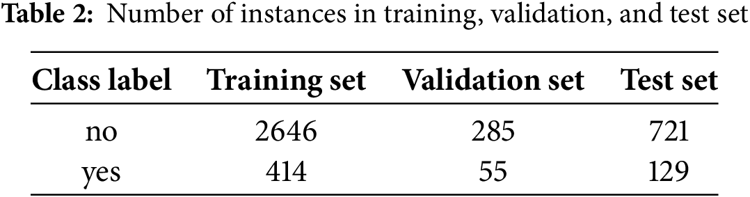
In this subsection, the experiments are conducted on the adopted dataset described in Section 3. It provides evidence supporting the effectiveness of the proposed model and interprets the results in a meaningful manner. First, the data preprocessing and splitting stage is applied to result in 18 features, including the class label, making the dataset clean, consistent, and suitable for input into the neural network. Table 2 presents the number of instances in the training set, validation set, and test set.

Additionally, at this stage, a visual representation of the pairwise correlation coefficients between all numerical features in the dataset is provided using a correlation heat map, as shown in Fig. 4. This helps uncover intuitive or surprising relationships among the features.

Figure 4: Number of instances based on the classes and their distribution

As shown in Fig. 4, the number_vmail_messages has a positive correlation, approximately 0.95, with the voice_mail_plan. This indicates a near-linear relationship. In other words, customers with a voicemail plan tend to have non-zero voicemail messages, while those without the plan typically have none. This relationship may negatively impact some models, particularly linear ones. However, the RBiLSTM may handle this redundancy without performance degradation. After compiling the proposed RBiLSTM model using TensorFlow and Keras libraries, Fig. 5 illustrates its architecture, highlighting its sequential layers, dropout regularization components, and output dense layer for binary churn classification.

Figure 5: RBiLSTM model architecture

To identify the most effective training setup, a hyper-parameter optimization process is carried out using grid search, with validation monitoring and validation loss used as indicators of the best generalization performance. The validation set is used to monitor training progress and prevent overfitting. The hyperparameter values of the optimization stage are given in Table 3, and the validation loss results for these values are demonstrated in Table 4.

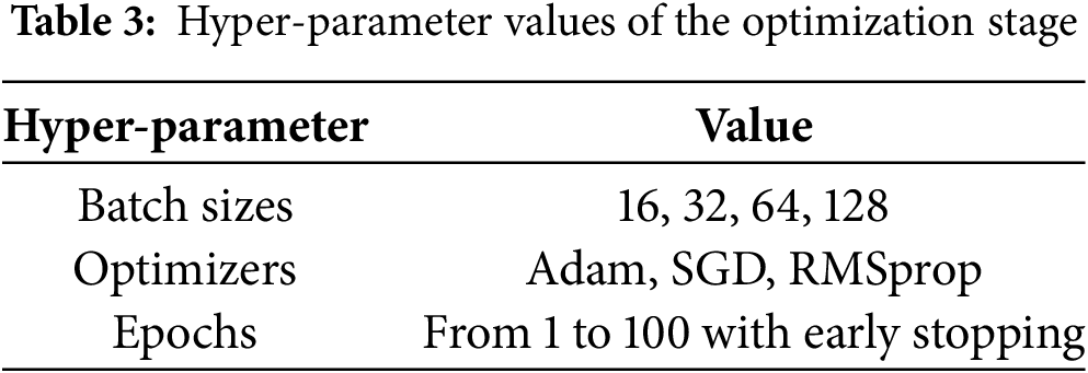
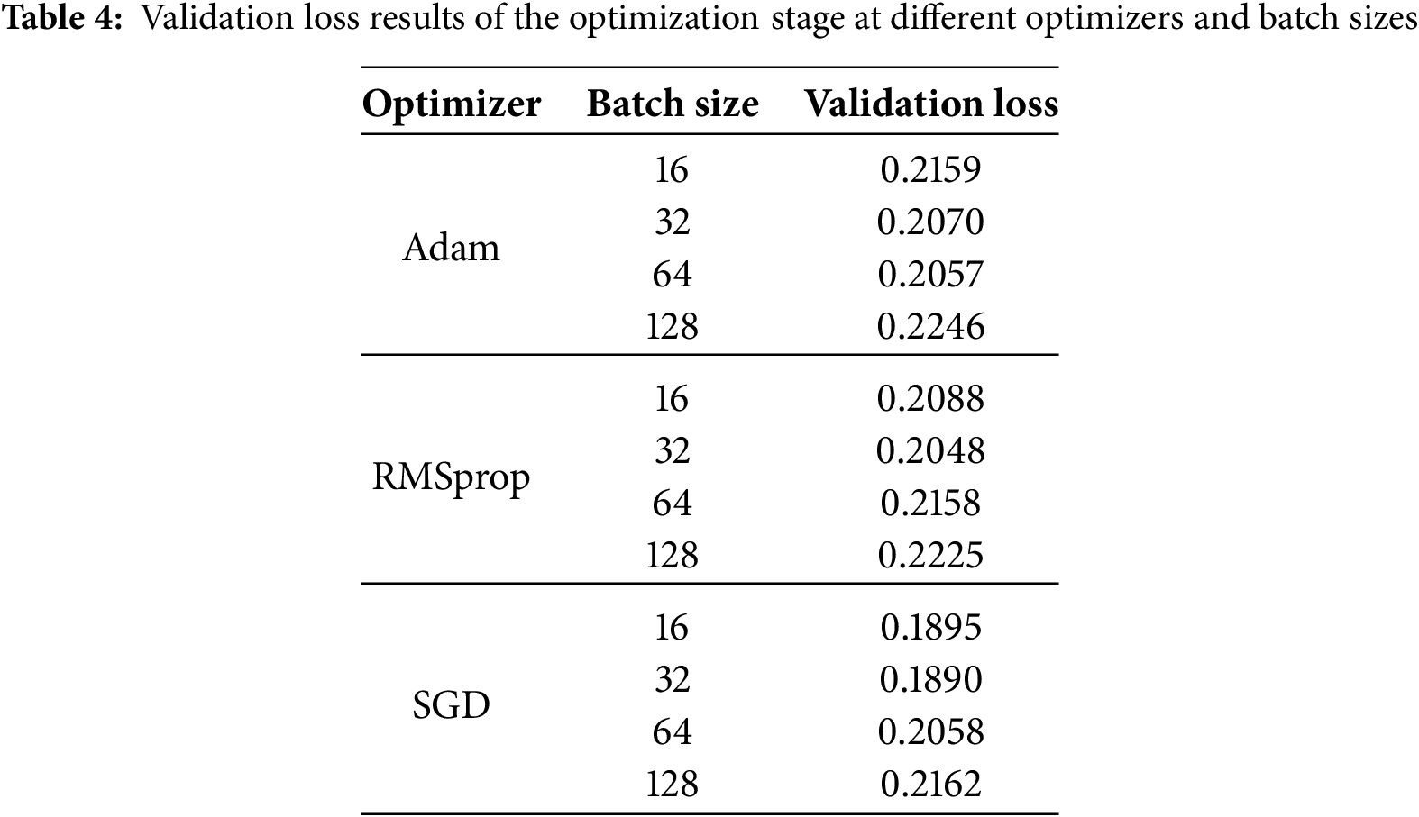
As shown in Table 4, the RBiLSTM model achieves the best validation loss, which is 0.1890, using the SGD optimizer and a batch size of 32, highlighted in bold font. These hyper-parameter values are used to train the model and ensure an optimal balance between convergence speed, generalization, and accuracy. Fig. 6 visualizes the curves of accuracy and loss for the training and validation sets using the SGD optimizer and a batch size of 32.

Figure 6: Training curves of the RBiLSTM model using SGD optimizer and 32 batch size: (a) accuracy curve of the training and validation sets; (b) loss curve of the training and validation sets

For correctly classified instances, Table 5 displays the confusion matrix of the test set for the RBiLSTM model trained using the optimal values of the optimizer and batch size with early stopping.

From the confusion matrix, we can see that 709 out of 721 instances with the ‘no churn’ class label are correctly classified as ‘no churn’, and 108 out of 129 instances with the ‘yes churn’ class label are correctly classified as ‘yes churn’. Therefore, the results of accuracy, macro, and weighted average F1-score for the model are 96.1%, 92.2%, and 96.1%, respectively, as shown in Table 6. Moreover, Fig. 7 visualizes the Receiver Operating Characteristic (ROC) Curve on the test set. It demonstrates the ability of RBiLSTM to achieve an AUC of 0.94, showcasing the model’s discriminative power.

Figure 7: Receiver Operating Characteristic (ROC) Curve of the test set for the RBiLSTM model

Based on the experimental results above, the 32-batch size and the SGD optimizer for the RBiLSTM provide the best balance between convergence speed, stability, and generalization. To provide a more accurate estimate of the model’s performance, a 10-fold cross-validation is conducted on the dataset through the experiments. The 10-fold cross-validation is a reliable model evaluation approach for assessing model’s generalization capability. This approach divides the dataset into ten equal-sized subsets, or folds. For each of the ten iterations, one fold is kept for testing, while the remaining nine folds are utilized to train the model. This method is performed ten times, with each fold serving as the test set only once. After all iterations, the results of evaluation metrics for all tested folds are averaged to yield a single, accurate measure of model performance. According to the 10-fold cross-validation, the RBiLSTM model achieved an average AUC of 0.918 and an average accuracy of 95.58%, which are almost identical to the evaluation results of the train-test split technique. Because the dataset is imbalanced, an additional experiment is conducted to investigate the effect of data augmentation using the Synthetic Minority Oversampling Technique (SMOTE) method on the model’s performance. The original training dataset shape before data augmentation was 2646 for the no class and 414 for the yes class. After applying the SMOTE method, the resampled training dataset’s shape became 2646 for the ‘no’ class and 2646 for the ‘yes’ class. The evaluation results of the RBiLSTM model on the test set are shown in Tables 7 and 8.

From Tables 7 and 8, we can see that the performance results of the RBiLSTM model using SMOTE on the training set are lower than the results without using the SMOTE method. This is because the synthetic samples may not accurately reflect real test data, causing the model to learn unrealistic patterns that do not exist in the test set, resulting in worse generalization and reduced accuracy, precision, recall, and overall F1-score results for the test set. The overlap between unrealistic synthetic yes patterns and the majority no patterns decreases the number of correctly classified instances for the no class from 709 to 676 instances, as shown in Table 7, resulting in a drop in accuracy to 92%. However, the number of correctly classified instances for the minority ‘yes’ class increased from 106 to 108 instances, as presented in Table 5, demonstrating the robustness of the model against synthetic samples that could represent new data in non-informative directions, adding more noise than real representative test data.

For explaining the predictions of the RBiLSTM model to business users, a SHAP (SHapley Additive exPlanations) method is used, highlighting the features that contributed most to that specific prediction outcome. It utilizes SHAP values, which originate from cooperative game theory, to assign a numerical value to each feature indicating its contribution to a particular prediction. This transparency is beneficial for business users who need to act upon RBiLSTM model outputs. Additionally, during the experiments, an ablation study is conducted to assess the impact of various components on the overall performance of the proposed RBiLSTM architecture. By systematically removing or changing model components, their impact on accuracy and F1-score key metrics is assessed. This ablation study aims to validate and identify the importance and effect of each architectural component, such as bidirectional layers and regularization with early stopping, and justify the selection of model design choices. In the experimental setup, the RBiLSTM model and some variations of its architecture, including the baseline dense layer, are trained on the training and validation sets and evaluated on the test set. Fig. 8 presents the SHAP values of features contributing to the prediction outcome of the RBiLSTM model for instances 1 and 15 in the test set. Table 9 shows the evaluation results of the ablation study in terms of accuracy and F1-score.

Figure 8: SHAP values for features contributed to the prediction outcome of the RBiLSTM model: (a) SHAP values for instance 1 in the test set predicted likely to churn; (b) SHAP values for instance 15 in the test set predicted likely no churn

As shown in Fig. 8b for the instance predicted as churn, we can notice that the voice_mail_plan feature has a positive SHAP value and contributes more strongly towards the churn prediction compared to its positive SHAP value for the instance predicted as no churn in Fig. 8a. It is noticed from Fig. 8a,b that the international_plan feature consistently has a substantial negative impact, strongly influencing the prediction towards no churn, and the number_customer_service_calls feature consistently has a substantial positive impact on the churn prediction, strongly influencing the prediction towards churn. Moreover, as shown in the ablation study documented in Table 9, the BiLSTM (32) layer improves the model’s ability to capture deeper sequential dependencies. Additionally, we can demonstrate that removing dropout, regularization, and early stopping results in a 3.68% drop in accuracy and a 0.036 decrease in F1-score, indicating their effectiveness in mitigating overfitting. Moreover, the model architecture using only the baseline dense layer yields poor results, resulting in a 9.28% drop in accuracy and a 0.12 decrease in F1-score. These poor results are due to the absence of sequential modeling, confirming the advantage of temporal learning. According to the ablation study, the best performance can only be achieved with the full BiLSTM model, incorporating regularization and early stopping. Every architectural improvement significantly enhances the accuracy and F1-score of churn prediction. For a more comprehensive analysis, a comparative study is conducted using several baseline machine learning models, including LR, DT, KNN, SVM, DNN, and LSTM, as listed in Table 10. Moreover, Table 11 compares the F1-score results of the deep learning models implemented in this study on the same dataset with those of the models introduced in recent studies [17,25,31,32].

The experiments demonstrate that the improved RBiLSTM significantly enhances churn prediction performance. By incorporating dropout, L2 Regularization, and early stopping techniques, overfitting is reduced, resulting in a test accuracy of 96.10%. The model outperformed traditional classifiers and recently proposed models, as indicated by the F1-score results in Tables 10 and 11. However, slight bias is observed in some feature-based predictions, indicating the need for fairness-aware training strategies. Moreover, integrating attention mechanisms can capture long-term dependencies more effectively.

5  Conclusion and Future Work

In this study, a Regularized Bidirectional Long Short-Term Memory (RBiLSTM) model is proposed for the customer churn prediction task, leveraging sequential deep learning capabilities to capture both past and future context within customer behavior data. The model is trained and tested on a publicly available dataset, specifically the Customer Churn Prediction 2020 dataset. It outperforms traditional machine learning baseline models, such as LR, DT, KNN, SVM, DNN, and LSTM, achieving an impressive accuracy of 96.10%. The performance of the BiLSTM model is improved due to its ability to model complicated temporal linkages and sequence dependencies in the dataset, as well as effective regularization procedures such as dropout and resilient preprocessing techniques. The experimental results supported the model’s dependability across key assessment measures, including accuracy, recall, precision, and F1-score, demonstrating that it can effectively reduce both false positives and false negatives, which is crucial in churn prediction scenarios.

This study demonstrates the capability of RBiLSTM-based architectures to predict customer turnover accurately and lays the groundwork for future enhancements and real-world deployment in customer business systems. By utilizing a bidirectional LSTM architecture with regularization, the proposed approach successfully captures temporal trends and minimizes overfitting, resulting in good predictive performance. It is helpful for business insights because it also uses SHAP for interpretability. However, generalizability may be limited by the model’s evaluation on a single dataset. Furthermore, ideal performance may be impacted by the limited fixed and default values of other models’ hyperparameters, such as the number of units, learning rate, and decay. Although the model produced impressive results, there remains potential for further development and exploration. Future work could include testing the approach on larger and more diverse datasets, such as time-series modeling for longer-term consumer behavior, and extending the model with attention mechanisms to enhance focus on key time steps. Incorporating automated hyperparameter tuning approaches, such as Bayesian optimization or evolutionary algorithms, could also improve performance. Finally, using other explainability tools, such as Local Interpretable Model-Agnostic Explanations (LIME), can provide more profound and more comprehensive insights into model behavior.

Acknowledgement: The author would like to express his gratitude to King Khalid University, Saudi Arabia, for providing administrative and technical support.

Funding Statement: The author received no specific funding for this study.

Availability of Data and Materials: The data supporting the findings of this study are openly available on Kaggle at https://www.kaggle.com/c/customer-churn-prediction-2020/data (accessed on 01 September 2025).

Ethics Approval: Not applicable.

Conflicts of Interest: The author declares no conflicts of interest to report regarding the present study.

References

1. Wagh SK, Andhale AA, Wagh KS, Pansare JR, Ambadekar SP, Gawande S. Customer churn prediction in telecom sector using machine learning techniques. J Results Control Optim. 2024;14(3):100342. doi:10.1016/j.rico.2023.100342. [Google Scholar] [CrossRef]

2. Suh Y. Machine learning based customer churn prediction in home appliance rental business. J Big Data. 2023;10(1):41. doi:10.1186/s40537-023-00721-8. [Google Scholar] [CrossRef]

3. Rane NL, Achari A, Choudhary SP. Enhancing customer loyalty through quality of service: effective strategies to improve customer satisfaction, experience, relationship, and engagement. Int Res J Mod Eng Technol Sci Total Environ. 2023;5(5):427–52. doi:10.11591/ijere.v3i3.6191. [Google Scholar] [CrossRef]

4. Bhattacharyya J, Dash MK. Investigation of customer churn insights and intelligence from social media: a netnographic research. Online Inf Rev. 2021;45(1):174–206. doi:10.1108/oir-02-2020-0048. [Google Scholar] [CrossRef]

5. Lappeman J, Franco M, Warner V, Sierra-Rubia L. What social media sentiment tells us about why customers churn. J Consum Mark. 2022;39(5):385–403. doi:10.1108/jcm-12-2019-3540. [Google Scholar] [CrossRef]

6. Saleh S, Saha S. Customer retention and churn prediction in the telecommunication industry: a case study on a Danish university. SN Appl Sci. 2023;5(7):173. doi:10.1007/s42452-023-05389-6. [Google Scholar] [CrossRef]

7. Moshed A, Al-Jabaly S. Enhancing marketing success in Jordanian telecom: strategic IoT integration and brand relationship management for maximized consumer loyalty. J Infrastruct Policy Dev. 2024;8(6):3858. doi:10.24294/jipd.v8i6.3858. [Google Scholar] [CrossRef]

8. Quach S, Thaichon P, Hewege C. Triadic relationship between customers, service providers and government in a highly regulated industry. J Retail Consum Serv. 2020;55(2):102148. doi:10.1016/j.jretconser.2020.102148. [Google Scholar] [CrossRef]

9. Wang C, Rao C, Hu F, Xiao X, Goh M. Risk assessment of customer churn in telco using fclcnn-lstm model. Expert Syst Appl. 2024;248(21):123352. doi:10.1016/j.eswa.2024.123352. [Google Scholar] [CrossRef]

10. Sedighimanesh M, Sedighimanesh A, Gheisari M. Optimizing hyperparameters for customer churn prediction with PSO-enhanced composite deep learning techniques. J Inf Syst Telecommun. 2025;50(13):91–111. doi:10.61882/jist.48088.13.50.91. [Google Scholar] [CrossRef]

11. Nalatissifa H, Pardede HF. Customer decision prediction using deep neural network on telco customer churn data. J Elektron Dan Telekomun. 2021;21(2):122–7. doi:10.14203/jet.v21.122-127. [Google Scholar] [CrossRef]

12. Capponi G, Corrocher N, Zirulia L. Personalized pricing for customer retention: theory and evidence from mobile communication. Telecommun Policy. 2021;45(1):102069. doi:10.1016/j.telpol.2020.102069. [Google Scholar] [CrossRef]

13. Mitchell WD. Proactive predictive analytics within the customer lifecycle to prevent customer churn [dissertation]. Scottsdale, AZ, USA: Northcentral University; 2020. [Google Scholar]

14. Sikri A, Jameel R, Idrees SM, Kaur H. Enhancing customer retention in telecom industry with machine learning driven churn prediction. Sci Rep. 2024;14(1):13097. doi:10.1038/s41598-024-63750-0. [Google Scholar] [CrossRef]

15. Bharadiya JP, Bharadiya J. Machine learning and AI in business intelligence: trends and opportunities. Int J Comput Sci Eng Surv. 2023;48(1):123–34. [Google Scholar]

16. Hassan A, Mhmood A. Optimizing network performance, automation, and intelligent decision-making through real-time big data analytics. Int J Responsible Artif Intell. 2021;11(8):12–22. [Google Scholar]

17. Wu S, Yau W-C, Ong T-S, Chong S-C. Integrated churn prediction and customer segmentation framework for telco business. IEEE Access. 2021;9:62118–36. doi:10.1109/access.2021.3073776. [Google Scholar] [CrossRef]

18. Lalwani P, Mishra MK, Chadha JS, Sethi P. Customer churn prediction system: a machine learning approach. Computing. 2022;104(2):271–94. doi:10.1007/s00607-021-00908-y. [Google Scholar] [CrossRef]

19. Dahiya K, Bhatia S, editors. Customer churn analysis in telecom industry. In: Proceedings of the 2015 4th International Conference on Reliability, Infocom Technologies and Optimization (ICRITO) (Trends and Future Directions); 2015 Sep 2–4; Noida, India. doi:10.1109/icrito.2015.7359318. [Google Scholar] [CrossRef]

20. Gattermann-Itschert T, Thonemann UW. Proactive customer retention management in a non-contractual B2B setting based on churn prediction with random forests. Ind Mark Manag. 2022;107:134–47. doi:10.1016/j.indmarman.2022.09.023. [Google Scholar] [CrossRef]

21. Pamina J, Raja B, SathyaBama S, Sruthi M, VJ A. An effective classifier for predicting churn in telecommunication. Jour Adv Res Dyn Control Syst. 2019;11(1):221–9. doi:10.13140/RG.2.2.35091.94249. [Google Scholar] [CrossRef]

22. Esteves G, Mendes-Moreira J, editors. Churn perdiction in the telecom business. In: Proceedings of the 2016 Eleventh International Conference on Digital Information Management (ICDIM); 2016 Sep 19–21; Porto, Portugal. doi:10.1109/icdim.2016.7829775. [Google Scholar] [CrossRef]

23. Tavassoli S, Koosha H. Hybrid ensemble learning approaches to customer churn prediction. Kybernetes. 2022;51(3):1062–88. doi:10.1108/k-04-2020-0214. [Google Scholar] [CrossRef]

24. Adhikary DD, Gupta D. Applying over 100 classifiers for churn prediction in telecom companies. Multimed Tools Appl. 2021;80(28):35123–44. doi:10.1007/s11042-020-09658-z. [Google Scholar] [CrossRef]

25. Imani M, Arabnia HR. Hyperparameter optimization and combined data sampling techniques in machine learning for customer churn prediction: a comparative analysis. Technologies. 2023;11(6):167. doi:10.3390/technologies11060167. [Google Scholar] [CrossRef]

26. Idris A, Rizwan M, Khan A. Churn prediction in telecom using Random Forest and PSO based data balancing in combination with various feature selection strategies. Comput Electr Eng. 2012;38(6):1808–19. doi:10.1016/j.compeleceng.2012.09.001. [Google Scholar] [CrossRef]

27. Sansana J, Joswiak MN, Castillo I, Wang Z, Rendall R, Chiang LH, et al. Recent trends on hybrid modeling for Industry 4.0. Comput Chem Eng. 2021;151(10):107365. doi:10.1016/j.compchemeng.2021.107365. [Google Scholar] [CrossRef]

28. Sharaf Addin EH, Admodisastro N, Mohd Ashri SNS, Kamaruddin A, Chong YC. Customer mobile behavioral segmentation and analysis in telecom using machine learning. Appl Artif Intell. 2022;36(1):2009223. doi:10.1080/08839514.2021.2009223. [Google Scholar] [CrossRef]

29. Wu X, Li P, Zhao M, Liu Y, Crespo RG, Herrera-Viedma E. Customer churn prediction for web browsers. Expert Syst Appl. 2022;209(1):118177. doi:10.1016/j.eswa.2022.118177. [Google Scholar] [CrossRef]

30. Bhattacharjee S, Thukral U, Patil N, editors. Early churn prediction from large scale user-product interaction time series. In: Proceedings of the 2023 International Conference on Machine Learning and Applications (ICMLA); 2023 Dec 15–17; Jacksonville, FL, USA. doi:10.1109/icmla58977.2023.00314. [Google Scholar] [CrossRef]

31. Beltozar-Clemente S, Iparraguirre-Villanueva O, Pucuhuayla-Revatta F, Zapata-Paulini J, Cabanillas-Carbonell M. Predicting customer abandonment in recurrent neural networks using short-term memory. J Open Innov Technol Mark Complex. 2024;10(1):100237. doi:10.1016/j.joitmc.2024.100237. [Google Scholar] [CrossRef]

32. Kumar MR, Priyanga S, Anusha JS, Chatiyode V, Santiago J, Chaudhary D, editors. Enhancing telecommunications customer retention: a deep learning approach using LSTM for predictive churn analysis. In: Proceedings of the 2024 International Conference on Data Science and Network Security (ICDSNS); 2024 Aug 23–24; Tiruchengode, India. doi:10.1109/icdsns62112.2024.10691038. [Google Scholar] [CrossRef]

33. Rudd DH, Huo H, Islam MR, Xu G, editors. Churn Prediction via multimodal fusion learning: integrating customer financial literacy, voice, and behavioral data. In: Proceedings of the 2023 10th International Conference on Behavioural and Social Computing (BESC); 2023 Oct 30–Nov 1; Larnaca, Cyprus. doi:10.1109/besc59560.2023.10386253. [Google Scholar] [CrossRef]

34. Bai S, Kolter JZ, Koltun V. An empirical evaluation of generic convolutional and recurrent networks for sequence modeling. arXiv:1803.01271. 2018. [Google Scholar]

35. Asfe AM, Rahman MR, Hossain MS. MNeuralTab: integrating meta-modeling and neural networks for customer churn prediction in e-commerce. Discov Appl Sci. 2025;7(6):569. doi:10.1007/s42452-025-07157-0. [Google Scholar] [CrossRef]

36. Asif D, Arif MS, Mukheimer A. A data-driven approach with explainable artificial intelligence for customer churn prediction in the telecommunications industry. Results Eng. 2025;26:104629. doi:10.1016/j.rineng.2025.104629. [Google Scholar] [CrossRef]

37. Liu Y, Shengdong M, Jijian G, Nedjah N. Intelligent prediction of customer churn with a fused attentional deep learning model. Mathematics. 2022;10(24):4733. doi:10.3390/math10244733. [Google Scholar] [CrossRef]

38. Ahmed U, Khan A, Khan SH, Basit A, Haq IU, Lee YS. Transfer learning and meta classification based deep churn prediction system for telecom industry. arXiv:1901.06091. 2019. [Google Scholar]

39. Diamantaras K. Customer churn prediction 2020 [Internet]; 2020 [cited 2025 Sep 1]. Available from: www.kaggle.com/c/customer-churn-prediction-2020/data. [Google Scholar]

40. Prihanditya HA. The implementation of z-score normalization and boosting techniques to increase accuracy of c4.5 algorithm in diagnosing chronic kidney disease. J Soft Comput Explor. 2020;1(1):63–9. [Google Scholar]

41. Balayla J. Performance metrics of binary classifiers. In: Theorems on the prevalence threshold and the geometry of screening curves: a bayesian approach to clinical decision-making. Berlin/Heidelberg, Germany: Springer; 2024. p. 129–42. [Google Scholar]