Cooperative Metaheuristics with Dynamic Dimension Reduction for High-Dimensional Optimization Problems

1  Introduction

Traditional gradient optimization algorithms, such as the steepest descent [1], Newton [2], and quasi Newton [3] methods, effectively utilize gradient information of the objective function, enabling rapid convergence and low computational cost. However, they are susceptible to converging on local optima rather than finding global optima. In practical engineering structural design, where optimization problems are typically high-dimensional and nonlinear, gradient methods are highly susceptible to converging to local optima, resulting in suboptimal solutions. To overcome these limitations, metaheuristic algorithms have emerged and have been employed in numerous fields, including machine learning hyperparameter optimization [4,5], path planning [6], scheduling problems [7], and structural optimization [8].

Metaheuristic algorithms require no gradient information and conduct global searches for optimal solutions, effectively avoiding local optima traps. These methods fall into two primary categories: swarm intelligence algorithms [9] and evolutionary algorithms [10]. Exhibiting strong robustness and adaptability, such algorithms are well-suited for complex engineering optimization problems and have emerged as powerful tools for solving high-dimensional nonlinear optimization challenges.

Swarm intelligence algorithms draw inspiration from the collective behaviors observed in bird flocks, fish schools, ant colonies, and bee swarms. Examples include particle swarm optimization (PSO) [11], ant colony optimization [12], and artificial bee colony algorithm [13]. Recently, Santhosh et al. [14] proposed a modified gray wolf optimization algorithm with feature selection to enable an effective prediction of Parkinson’s disease. Wei et al. [15] developed an improved whale optimization algorithm incorporating multi-strategy to address engineering design challenges. Addressing data classification challenges, Bangyal et al. [16] employed a modified bat algorithm with strengthened exploitation capability to mitigate the issue of convergence to local minima. Later, the same authors [17] introduced a modern computerized bat algorithm to examine a comprehensive set of benchmark test functions.

Among these swarm intelligence algorithms, PSO has garnered significant popularity for its conceptual simplicity and ease of implementation [18]. The original formulation of the PSO algorithm was presented by Eberhart and Kennedy [19], and then improved by many researchers. Chen et al. [20] and Ge et al. [21] developed random mutation modifications to enhance search capabilities of PSO. After that, Bala et al. [22] proposed an improved PSO framework with orthogonal initialization and a crossover mechanism to improve both the exploration capability and global search performance. However, these algorithms are often computationally intensive, particularly in the context of optimization problems with high dimensions, strong nonlinearities and complex constraints.

Unlike swarm intelligence algorithms, evolutionary algorithms are modeled on the principles of biological evolution (natural selection, genetic inheritance, and mutation). Examples include differential evolution (DE) [23], genetic algorithm [24], and evolution strategy [25]. DE is particularly prevalent in current literature for simple program implementation and fewer adjustment parameters [26]. Storn and Price [27] originally proposed the DE algorithm. The algorithm is initially intended for continuous variables and further developed to handle discrete variables. Ho-Huu et al. [28] and Vo-Duy et al. [29] proposed adaptive elitist DE, which has demonstrated improved precision and efficiency for discrete and composite optimization problems. Despite these advancements, computational demands remain high, even for relatively high-dimensional optimization problems.

To tackle these issues, researchers have developed innovative strategies to enhance the performance of metaheuristic algorithms for high-dimensional problems. Carlsson et al. [30] employed the eigenstructure of the Hessian for dimension reduction (DR) in intensity modulated radiation therapy optimization, while Fernández Martínez and García Gonzalo [31] applied principal components analysis (PCA) to reduce dimensions of inverse problems. As evidenced by the aforementioned literature, different DR strategies are often combined with metaheuristic algorithms to tackle high-dimensional challenges.

To efficiently solve high-dimensional optimization problems, cooperative metaheuristics with a dynamic DR strategy (C-PSO and C-DE) are developed based on the metaheuristic algorithms (PSO and DE). In the proposed methods, the modified PCA is utilized to reduce the dimension of design variables, thereby decreasing computational costs. The dynamic DR strategy implements periodic execution of modified PCA after a fixed number of iterations, resulting in the important dimensions being dynamically identified. Compared with the static one, the dynamic DR strategy can achieve precise identification of important dimensions, thereby enabling accelerated convergence toward optimal solutions. Furthermore, the effect of different thresholds of cumulative contribution rate on optimization problems with different dimensions is investigated. Though the threshold for a specific problem is set empirically, the adjustability of the threshold can guarantee the robustness of the cooperative methods. These strategies collectively enhance the computational efficiency and solution accuracy of the cooperative metaheuristics.

The primary advancements in this research are threefold: (1) unlike existing PCA, the modified PCA focuses on the correlation coefficients between variables and fitness values rather than the eigenvalues; (2) as the optimization progresses, the important dimensions will dynamically change; (3) the cumulative contribution rate threshold is investigated to determine the important dimensions.

This paper is organized as follows. Section 2 presents a review of the metaheuristic algorithms. Section 3 describes the cooperative metaheuristics. In Section 4, 15 benchmark test functions are first examined, then a speed reducer and a composite pressure vessel design problem are performed to demonstrate the efficacy of the cooperative methods. Section 5 gives the conclusions.

2  Review of the Metaheuristic Algorithms

PSO is a typical swarm intelligence algorithm, whereas DE represents a classical evolutionary algorithm. These two representative metaheuristic algorithms are employed in this article owing to their simple program implementation, other metaheuristic algorithms can also be incorporated with the DR strategy. PSO has been studied excessively, readers are encouraged to consult reference [32] for comprehensive details.

The DE framework comprises four key steps [23]: initialization, mutation, crossover, and selection. As a parallel direct search method, a population of N individuals in an n-dimensional space at generation k is represented by xik = (xi,1k, xi,2k, …, xi,nk), i = 1, 2, …, N. The specific procedure of the DE algorithm is outlined below:

Step 1: Initialization.

A randomly generated population is created throughout the entire design space. And the new generation of the population is developed by the following steps.

Step 2: Mutation.

During this step, a mutant vector is generated by combining a weighted differential between two population members with a third individual:

vik+1=xr1k+F×(xr2k−xr3k)(1)

where the random indices r1, r2, r3 should be distinct integers, and the constant F ∈ [0, 2] serves as a real-valued coefficient that determines the magnitude of differential variation (xr2k–xr3k). Additionally, the index i should be different from r1, r2, r3. As a result, the population size N must be at least four.

Step 3: Crossover.

A crossover process is employed to increase population diversity. Following the crossover, a trial individual is generated as uik+1 = (ui,1k+1, ui,2k+1, …, ui,nk+1). The crossover operation is defined as follows:

ui,jk+1={vi,jk+1,r(j)≤CR orj=r(i)xi,jk,otherwise(2)

in which r(j) represents a randomly generated value corresponding to the j-th dimension, which is uniformly distributed within the range [0, 1]; CR is a user-specified crossover rate, bounded between 0 and 1; while r(i) denotes an index chosen stochastically from the set {1, 2, …, n} that ensures the trial individual uik+1 inherits at least one parameter from the mutant individual vik+1.

Step 4: Selection.

The selection operation is employed to retain individuals with better evaluation function values. In this way, the population can progressively converge toward the optimum. The selection operation is given by:

xik+1={uik+1,f(uik+1)≤f(xik)xik,otherwise(3)

where f() is the evaluation function.

3  The Proposed Cooperative Metaheuristics

As previously mentioned, metaheuristic algorithms are often incorporated with different DR strategies to address high-dimensional optimization challenges. Common DR strategies include: PCA [31], Kernel PCA [33], independent component analysis [34], and t-distributed stochastic neighbor embedding [35]. Compared to these alternatives, PCA offers superior computational efficiency and implementation simplicity, motivating its adoption in this study.

3.1 The Basic PCA

High-dimensional data often presents complex patterns, which makes graphical representation challenging. In such scenarios, PCA is an invaluable technique in data analysis, notably for its capability to reveal underlying data patterns while allowing for DR without significant loss of information. The detailed procedure for performing PCA on a dataset is as follows:

Step 1: Obtain the data.

In this step, an n-dimensional dataset is utilized to illustrate the entire PCA procedure. The variables are denoted as Xi, i = 1, 2, …, n with the corresponding dataset represented as:

[x1x2⋯xn]=[x1,1x1,2⋯x1,nx2,1x2,2⋯x2,n⋮⋮⋱⋮xm,1xm,2⋯xm,n](4)

where m is the size of the dataset, and xi = [x1,i, x2,i, …, xm,i]T are the data of the variable Xi.

Step 2: Subtract the mean.

To center the data, we subtract the mean of each variable from the corresponding data, resulting in a dataset with a mean of zero:

[x1′x2′⋯xn′]=[x1,1−x¯1x1,2−x¯2⋯x1,n−x¯nx2,1−x¯1x2,2−x¯2⋯x2,n−x¯n⋮⋮⋱⋮xm,1−x¯1xm,2−x¯2⋯xm,n−x¯n](5)

where x¯i = (x1,i + x2,i + … + xm,i)/m is the mean of the data xi.

Step 3: Calculate the covariance matrix.

Cov=[cov(X1,X1)cov(X1,X2)⋯cov(X1,Xn)cov(X2,X1)cov(X2,X2)⋯cov(X2,Xn)⋮⋮⋱⋮cov(Xn,X1)cov(Xn,X2)⋯cov(Xn,Xn)](6)

where each covariance term can be calculated using the formula:

cov(Xi,Xj)=xi′⋅xj′m−1=∑k=1mxk,i′xk,j′m−1(7)

Step 4: Compute the eigenvalues and corresponding eigenvectors for the covariance matrix.

eigenvlaues:λ1,λ2,…,λn(8)

eigenvectors:eig1=[a1,1a2,1⋮an,1],eig2=[a1,2a2,2⋮an,2],…,eign=[a1,na2,n⋮an,n](9)

Step 5: Construct the principal components.

These new variables can be expressed in terms of the eigenvectors:

Fi=ai,1X1+ai,2X2+…+ai,nXn,i=1,2,…,n(10)

Step 6: Determine the contribution rate of each principal component.

Based on the eigenvalues, the contribution rate of each principal component is calculated using the formula:

Ci=λi∑j=1nλj,i=1,2,…,n(11)

in which Ci denotes the contribution rate corresponds to the i-th principal component. These rates inform the selection of the most significant components for analysis, while those with minimal contributions are typically excluded to streamline the process.

3.2 The Modified PCA

As previously mentioned, the contribution rates of principal components can be utilized to select certain dimensions for analysis. When addressing a high-dimensional optimization problem, it is feasible to identify and retain only the most important dimensions as the design variables. In this context, the modified PCA diverges slightly from the basic PCA.

In basic PCA, each dimension is interrelated, meaning that the dimensions can influence each other. Conversely, in optimization problems, while each dimension does affect the function value, they do not have direct influences on one another. To adapt this concept for optimization, the modified PCA is developed to calculate contribution rates using the correlation coefficients between each dimension and the function value, rather than the eigenvalues. Subsequently, we can select the most important dimensions for the optimization process. The detailed procedure is outlined below.

Consider an n-dimensional optimization problem represented by the following formulation:

min:f(X)where:X=[X1,X2,…,Xn]subject to:gj(X)≤0,j=1,2,…,lXi,min≤Xi≤Xi,max,i=1,2,…,n(12)

in which X is a vector of n-dimensional design variables; f(X) represents the objective function; while gj(X) ≤ 0 defines the j-th constraint; Xi is bounded by Xi,min and Xi,max.

The implementation procedure for the modified PCA is described below:

Step 1: Obtain the data.

The (n + 1)-dimensional data can be obtained by:

[x1,1x1,2⋯x1,nf1x2,1x2,2⋯x2,nf2⋮⋮⋱⋮⋮xm,1xm,2⋯xm,nfm](13)

where m is the size of the data, and xi = [x1,i, x2,i, …, xm,i]T are the data of the variable Xi; fj = f(xj,1, xj,2, …, xj,n) is the function value of the j-th data.

Step 2: Compute the correlation coefficients.

The correlation coefficients between each dimension and the function value can then be calculated as follows:

cor(Xi,f)=∑j=1m(xj,i−x¯i)(fj−f¯)∑j=1m(xj,i−x¯i)2∑j=1m(fj−f¯)2,i=1,2,…,n(14)

where x¯i = (x1,i + x2,i + … + xm,i)/m is the mean of the data xi; f¯ = (f1 + f2 + … + fm)/m is the mean of all function values f.

Step 3: Calculate the contribution rates.

The contribution rates can then be determined as follows:

Ci=|cor(Xi,f)|∑j=1n|cor(Xj,f)|,i=1,2,…,n(15)

Step 4: Sort the contribution rates and calculate the cumulative contribution rates.

The contribution rates are sorted in descending order, and it is assumed that C1′,C2′, …, Cn′ represent these sorted values with X1′, X2′, …, Xn′ being the corresponding design variables. The cumulative contribution rate is then calculated using the following formula:

CTk=∑i=1kCi′,k=1,2,…,n(16)

Step 5: Select the important dimensions.

At this stage, the important dimensions can be selected based on a predefined threshold for the cumulative contribution rate Cth. The important dimensions are determined until the cumulative contribution rate reaches or exceeds the critical value Cth. For instance, if CTk−1 < Cth and CTk ≥ Cth, the variables X1′, X2′, …, Xk′ are then determined as the important dimensions, while the variables Xk+1′, Xk+2′, …, Xn′ are neglected.

Dynamic DR strategy implements periodic execution of modified PCA after a fixed number of iterations to dynamically identify the important dimensions. The important dimensions are chosen according to the threshold, so that variables with cumulative contribution rates exceeding the specified threshold are selected as important dimensions. However, the contribution rates of variables may vary with each iteration, ultimately leading to dynamic changes in cumulative contribution rates and important dimensions. During initial optimization stages, limited data availability compromises accurate identification of important dimensions, adversely affecting solution quality. As optimization progresses, accumulating data enables dynamic adjustment mechanisms to achieve precise identification of important dimensions, thereby enabling accelerated convergence toward optimal solutions.

3.3 The Cooperative Metaheuristics and the Procedure Description

Once the cumulative contribution rate threshold Cth is defined, the dimensions can be classified, allowing for the selection of important dimensions to serve as design variables in the optimization problem. The cooperative approaches integrate dynamic DR strategy with metaheuristic algorithms to effectively reduce computational costs meanwhile ensure solution precision.

The procedure for implementing the cooperative method can be outlined as follows (considering an n-dimensional problem with m data points):

Step 1: Generate an initial population.

An initial population with size m is first generated, these individuals are denoted as xi = [x1,i, x2,i, …, xm,i]T, i = 1, 2, …, n.

Step 2: Evaluate the fitness values.

Corresponding fitness values f = [f1, f2, …, fm]T, fj = f(xj,1, xj,2, …, xj,n), j = 1, 2, …, m are evaluated.

Step 3: Calculate the correlation coefficients.

Based on the data shown in Eq. (13), the correlation coefficients cor(Xi, f) between Xi and f are then calculated using Eq. (14).

Step 4: Calculate the contribution rates.

The contribution rates Ci are computed using Eq. (15).

Step 5: Sort the contribution rates and calculate the cumulative contribution rates.

Sort the contribution rates as C1′, C2′, …, Cn′ and calculate the cumulative contribution rates CTk using Eq. (16).

Step 6: Classify the dimensions based on the cumulative contribution rates.

Suppose that CTk−1 < Cth and CTk ≥ Cth, X1′, X2′, …, Xk′ are determined as the important dimensions, while Xk+1′, Xk+2′, …, Xn′ are neglected dimensions. Corresponding data become Xi′ = [X1,i′, X2,i′, …, Xm,i′]T, i = 1, 2, …, n.

Step 7: Define the optimization problem after DR.

Treat the important dimensions X1′, X2′, …, Xk′ as design variables and treat the neglected dimensions Xk+1′, Xk+2′, …, Xn′ as constants. In this way, the n-dimensional optimization problem is reduced to a k-dimensional optimization problem.

Step 8: Utilize the metaheuristic algorithms to update the population.

Employ the specified optimization algorithm (PSO, DE) to tackle the k-dimensional optimization problem, resulting in a new population denoted as pi′ = [p1,i′, p2,i′, …, pm,i′]T, i = 1, 2, …, k. The new population for the n-dimensional optimization problem is then defined as p1′, p2′, …, pk′, Xk+1′, Xk+2′, …, Xn′.

Step 9: Determine whether the optimization process is terminated.

The optimization process terminates when either the convergence criterion is satisfied or the maximum iteration count is exhausted, outputting the current solution as optimal. If neither condition is met, the algorithm reverts to Step 2.

Fig. 1 illustrates the comprehensive flowchart of the optimization procedure.

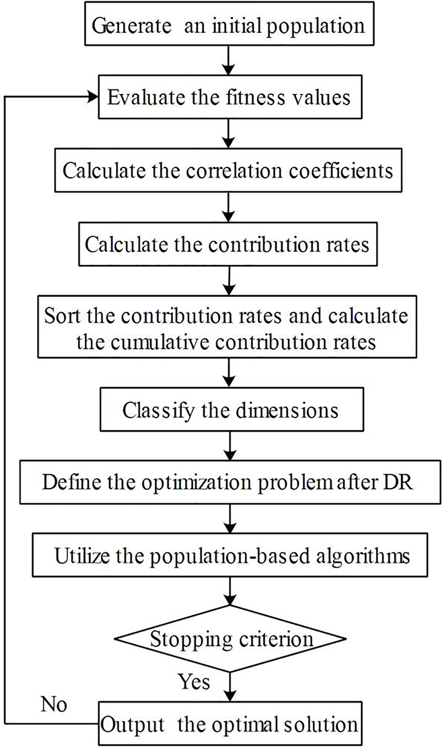
Figure 1: The flowchart of the cooperative metaheuristics

4  Numerical Applications

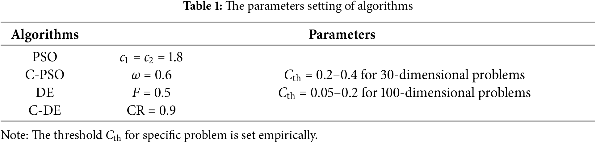
The parameters used in metaheuristic algorithms (PSO, DE) and cooperative methods (C-PSO, C-DE) are first defined. The population size and maximum number of iterations are specified as 200 for PSO and DE. In C-PSO and C-DE, the population size is reduced to 20, and the number of iterations for DR is set 20, i.e., the dynamic DR strategy is performed after every 20 iterations. The other parameters setting of algorithms are detailed in Table 1.

To assess the overall performance of all algorithms, different algorithms (PSO, DE, C-PSO, and C-DE) are independently run 30 times for all examples.

4.1 Benchmark Functions

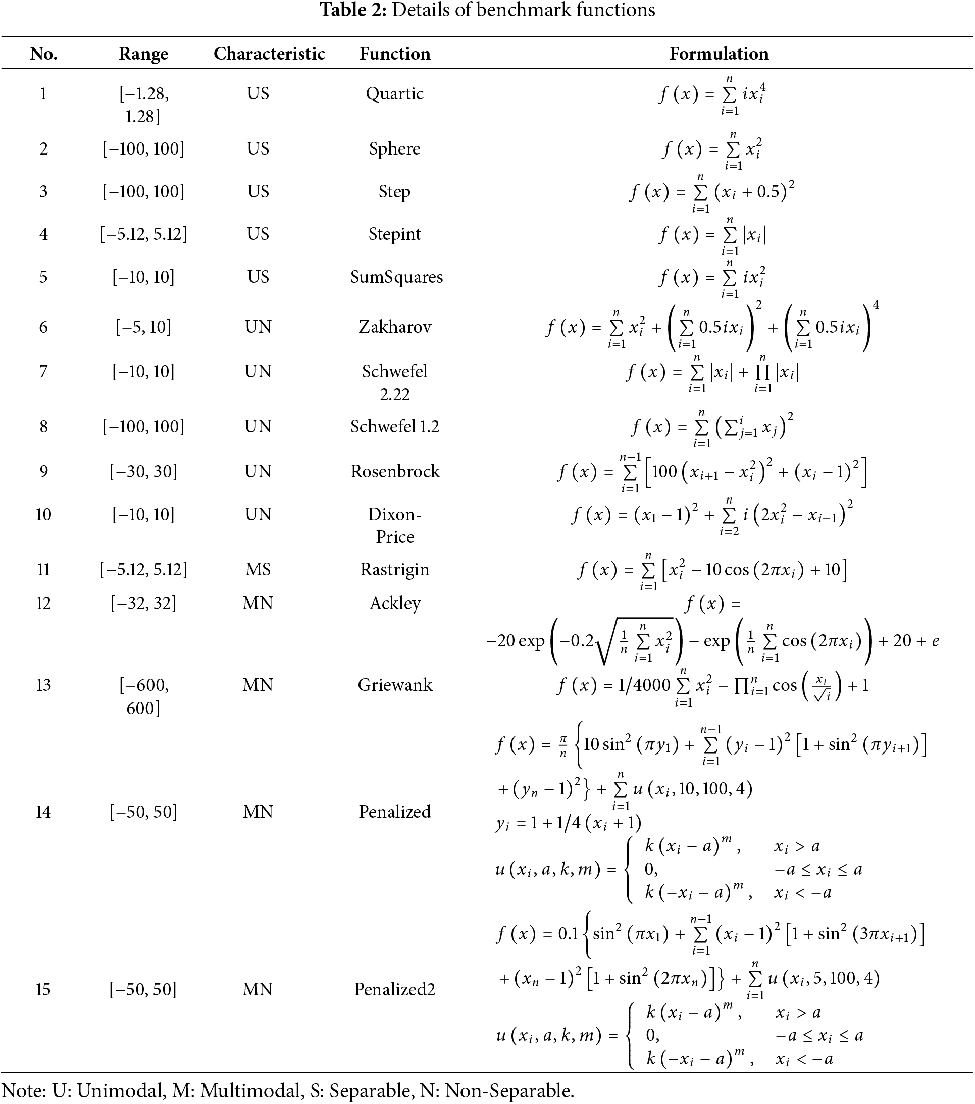
Within evolutionary computation, algorithmic performance is typically assessed through benchmark testing. For this purpose, 15 benchmark functions [36] are employed to examine the proposed C-PSO and C-DE algorithms. These test functions cover various problem types, comprising unimodal, multimodal, separable, and non-separable characteristics. The specifics of the variable ranges, problem characteristics, function types, and formulations are summarized in Table 2.

The optimizations are conducted for both 30-dimensional and 100-dimensional problems as detailed in Table 2. Comparative results from 30 individual runs for all benchmark functions are presented in Table 3. Notably, ‘Mean’ reflects the solution quality. For minimization problems, a lower ‘Mean’ indicates superior algorithm performance. ‘SD’ serves as a robustness indicator, where a smaller value demonstrates higher algorithmic stability. ‘N.F.’ measures computational efficiency, with fewer evaluations signifying greater efficiency. Since the execution time of the algorithm itself is negligible compared to that of response function evaluations or finite element analyses, the number of function calls or finite element program calls serves as a direct indicator of computational efficiency. Consequently, training and testing times are not reported herein.

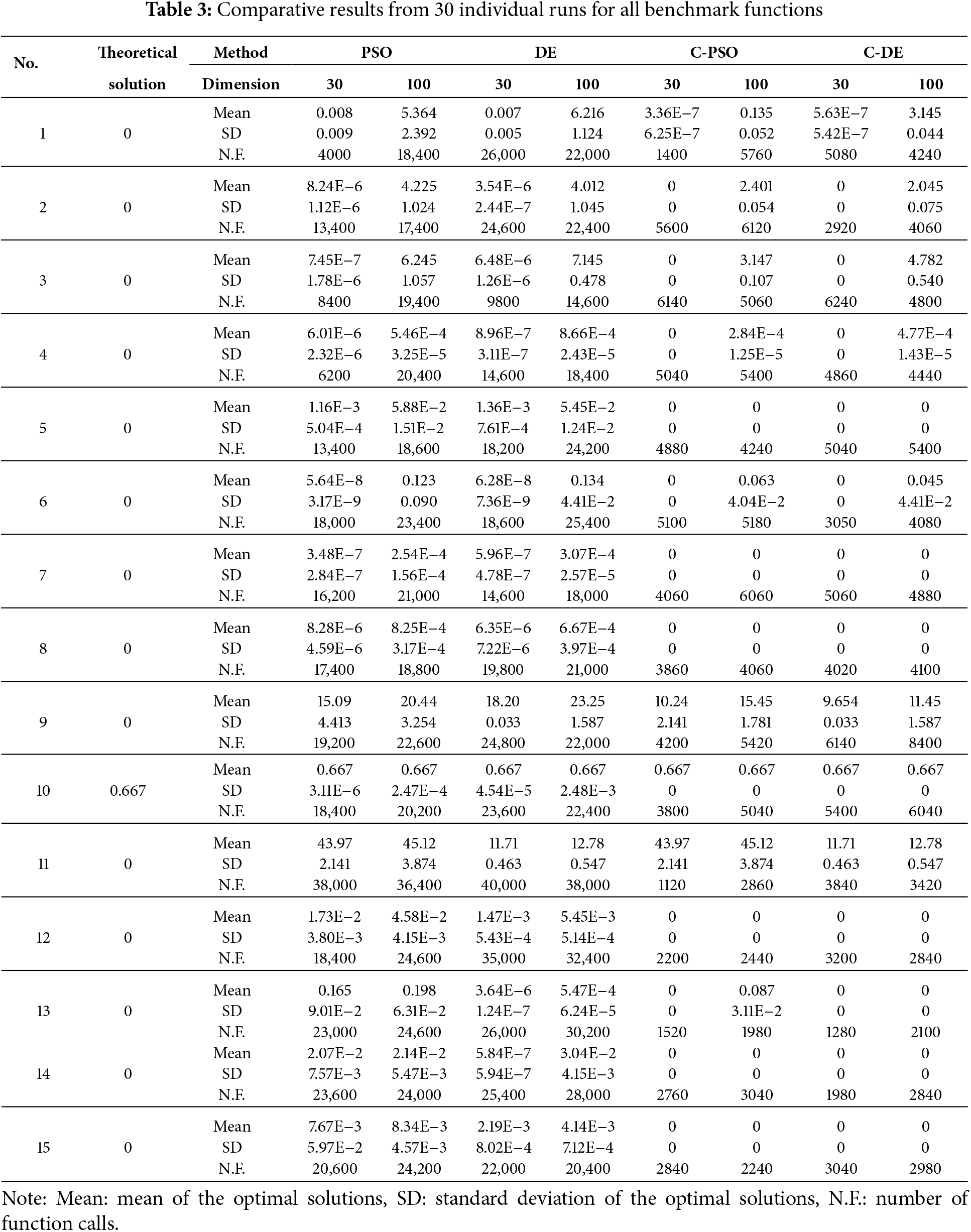
The results clearly indicate declining solution accuracy across all algorithms with increasing dimension. Compared to standard PSO and DE, both C-PSO and C-DE achieve better optimization solutions. For 30-dimensional problems, the cooperative methods attain theoretical optimal solutions for all test functions with the exception of Nos. 9 and 11. However, for 100-dimensional problems, C-PSO and C-DE can obtain theoretical optimal solutions for the majority of functions (Nos. 4, 5, 7, 8, 10, and 12–15), demonstrating their remarkable efficacy in addressing high-dimensional optimization tasks.

For the MN functions (Nos. 12–15), both PSO and DE can achieve good optimization results, while C-PSO and C-DE can obtain theoretical optimal solutions. Conversely, for the MS function (No. 11), all methods fail to obtain satisfactory results. Nevertheless, C-PSO and C-DE notably achieve better solutions than the standard methods. This demonstrates that the cooperative metaheuristics substantially enhance solution precision even for challenging optimization problems.

According to the preceding analysis, a critical limitation is revealed: both standard metaheuristics (PSO, DE) and their cooperative variants (C-PSO, C-DE) exhibit poor performance for multimodal separable optimization problems, particularly in high-dimensional cases.

Beyond solution quality, robustness serves as a critical performance metric for evaluating algorithmic efficacy. As evidenced in Table 3, the proposed methods achieve low ‘SD’ values across diverse test functions, with ‘SD’ = 0 observed in several cases, demonstrating exceptional robustness. Furthermore, ‘N.F.’ values of C-PSO and C-DE are always lower than those of PSO and DE for all benchmark functions, showing that the cooperative metaheuristics require less computational cost and have higher computational efficiency.

As described in Sections 3.2 and 3.3, the cumulative contribution rate threshold Cth is the decisive factor in defining important dimensions. Therefore, the effect of different thresholds on optimization problems with different dimensions is investigated. The results of Sphere function (No. 2 in Table 2) are given in Table 4.

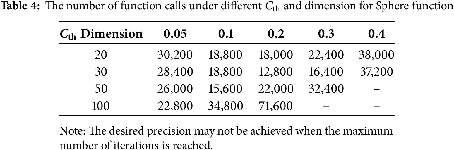
Table 4 demonstrates that the threshold Cth is not necessarily set as small as possible. For the low-dimensional problems, a too small threshold can lead to excessive information loss during DR, slowing down the optimization process. For high-dimensional problems, a small threshold can accelerate the optimization process in the early stage. The best outcomes for each dimension in Table 4 are highlighted in bold. As the dimension increases, the threshold needs to be set smaller to accelerate convergence and achieve optimal solutions more rapidly. Though the threshold for specific problem is set empirically, the adjustability of threshold can guarantee the robustness of the method.

4.2 A Speed Reducer Design

To further demonstrate the efficacy of the cooperative optimization algorithms, a more complex example involving a speed reducer design problem [20] is examined. The problem consists of seven dimensions, where x3 is an integer variable while all other variables remain continuous. The problem is structured as follows:

min:f(x)=0.7854x1x22(3.3333x32+14.9334x3−43.0934)−1.508x1(x62+x72)+7.4777(x63+x73)+0.7854(x4x62+x5x72) where:x=[x1,x2,…,x7]subject to:g1(x)=27x1x22x3−1≤0,g2(x)=397.5x1x22x32−1≤0,g3(x)=1.93x43x2x3x64−1≤0g4(x)=1.93x53x2x3x74−1≤0,g5(x)=x2x340−1≤0,g6(x)=5x2x1−1≤0g7(x)=x112x2−1≤0,g8(x)=1.5x6+1.9x4−1≤0,g9(x)=1.1x7+1.9x5−1≤0g10(x)=(745x4x2x3)2+16.9×106110x63−1≤0,g11(x)=(745x5x2x3)2+157.5×10685x73−1≤0(17)

where,

2.6≤x1≤3.6,0.7≤x2≤0.8,17≤x3≤287.3≤x4≤8.3,7.8≤x5≤8.3,2.9≤x6≤3.95≤x7≤5.5(18)

This is a single-objective problem with 11 behavioral constraints. PSO, DE, and their cooperative counterparts, C-PSO and C-DE, are all employed to solve this problem. Their results are compared with those of ‘Taguchi’ and ‘Sociobehavioural’ from the literature [20], as presented in Table 5. ‘Taguchi’ adopts a varing probe length value, which is initialized at 0.9 and reduced by one-half whenever the search direction shows no improvement. Meanwhile, ‘Sociobehavioural’ is executed using a population size of 100 over 200 iterations.

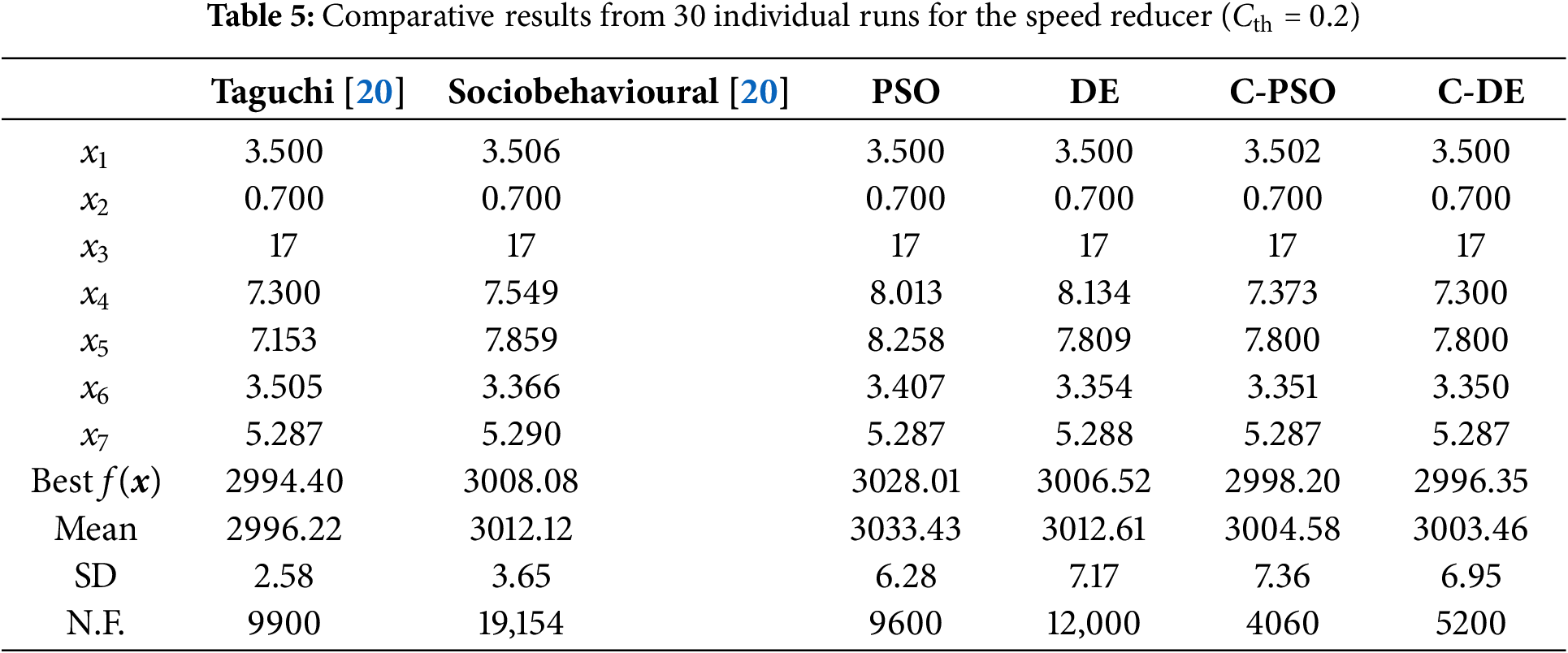
‘Best f(x)’ reflects the best solution among 30 individual runs. In minimization problems, a superior solution corresponds to a lower value. As evidenced in Table 5, C-PSO (2998.20) and C-DE (2996.35) significantly outperform PSO (3028.01) and DE (3006.52), confirming superior performance of the cooperative methods.

In terms of algorithmic robustness, ‘SD’ values of all algorithms are very small, which verifies the robustness of these methods. Meanwhile, ‘N.F.’ values of C-PSO (4060) and C-DE (5200) are significantly less than those of PSO (9600) and DE (12,000), indicating that the cooperative methods require less computational cost and have higher computational efficiency.

In summary, the proposed methods demonstrate superior solutions with reduced computational costs compared to the standard algorithms. This example illustrates the efficacy of the cooperative methods in tackling constrained optimization challenges. The convergence process of different algorithms are provided in Fig. 2.

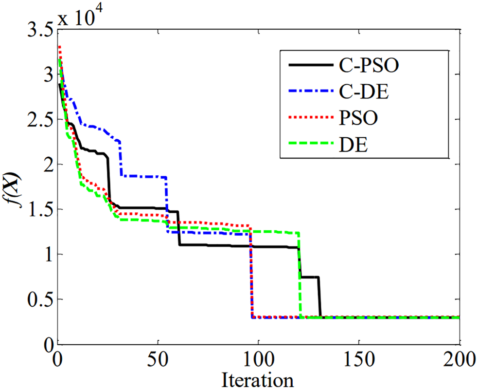
Figure 2: Convergence procedure for the speed reducer

It can be seen that PSO and DE no longer change after convergence, at which point the optimal solution is obtained. The convergence process of such algorithms is almost a one-time convergence solution without any sudden changes. The convergence process of C-PSO and C-DE is clearly a stepwise multiple convergence, mainly because in these two algorithms, the number of design variables dynamically changes with the intervention of the DR strategy.

4.3 A Composite Pressure Vessel Design

This study addresses a composite pressure vessel design problem [37], analyzing a Type 4 compressed hydrogen storage tank wrapped with carbon fiber. To ensure safety, the tank is designed with a safety factor of 2.25, resulting in a minimum burst pressure requirement of 158 MPa. The Toray T700S carbon fiber is used with a rated tensile strength of 4900 MPa, and the fiber-resin composite (60% fiber volume fraction) exhibits a tensile strength of 2550 MPa. The density of the composite material is 1800 kg/m3. The liner of the vessel is made from high-density polyethylene (HDPE), with a thickness of 5 mm. The material properties are summarized in Table 6.

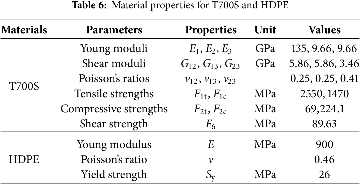
Fig. 3 illustrates a schematic of a storage tank with 521 mm diameter and 1.5 length-to-diameter (L/D) ratio, designed for 5.6 kg usable hydrogen capacity (5.8 kg total) at 70 MPa operating pressure. The tank features 15° helical winding layers and 90° hoop wound layers. During fabrication, helical and hoop layers are applied alternately over the liner to minimize resin pooling.

Figure 3: Schematic of a Type 4 compressed hydrogen storage tank

Fig. 4 shows the winding angle θ0 at the cylinder and θ at the head. These angles are calculated as follows:

θ0=arcsin⁡(rR0),θ=arcsin⁡(rR)(19)

where r represents the outer radius of the vessel, R0 denotes the outer radius of the cylindrical section, and R signifies the outer radius of the head at a specific location.

Figure 4: Geodesic fiber path along a pressure vessel surface

Finite element analysis (FEA) is performed using ANSYS, with the SHELL99 element modeling composite materials. This 8-node element features six degrees of freedom per node (translations and rotations in x, y, z directions). The SOLID191 element is used to simulate liner materials, with 20 nodes and three translational degrees of freedom per node (x, y, and z directions). The total number of elements in the model is 1650.

The design variables comprise thicknesses of five helical and four hoop layers, each ranging from 0.127 mm to 10 mm. The objective is to minimize the weight of the composite structure, subject to the constraint imposed by the Tsai-Wu strength criterion. The mathematical expression for this problem is:

min:W(d)where:d=[d1,d2,…,d9]subject to:|σ|≤σmax(20)

where W(d) is the total weight of the pressure vessel, and d is the thicknesses of nine layers, including five helical and four hoop layer thicknesses.

Comparative results obtained by 30 individual runs for the composite vessel are summarized in Table 7. The results are compared with those of genetic algorithm [37]. The population size and maximum number of iterations for genetic algorithm are set 200 and 100, respectively. The crossover probability is defined as 0.85 and the mutation probability is given as 0.0001.

‘Best W(d)’ denotes the best solution across 30 independent runs. For minimization problems, a superior solution is characterized by a smaller value. Table 6 demonstrates that C-PSO (103.6) and C-DE (103.1) achieve significantly better solutions than PSO (106.3) and DE (105.6), confirming superior performance of the cooperative methods. This advantage mainly stems from design space simplification: despite nine design variables, they resolve to just two parameter types (helical and hoop layer thicknesses), reducing inherent problem complexity.

Regarding algorithmic robustness, consistently low ‘SD’ values across all methods confirm exceptional solution stability. Computationally, the cooperative methods demonstrate superior efficiency: C-PSO reduces ‘N.F.’ values by 41.7% (10,400 → 6060), while C-DE achieves 48.5% reduction (9600 → 4940). Consequently, FEA calls decrease substantially, lowering computational costs. In summary, the proposed cooperative methods achieve superior solutions with better efficiency compared to the standard algorithms.

5  Conclusions

Based on standard metaheuristics PSO and DE, this paper presents cooperative metaheuristics C-PSO and C-DE that integrate dynamic DR. The modified PCA is utilized to reduce the dimension of design variables, thereby lowering computational costs. The dynamic DR strategy implements periodic execution of modified PCA after a fixed number of iterations, enabling dynamic identification of important dimensions. Compared to a static strategy, this dynamic implementation achieves precise identification of important dimensions, thereby driving accelerated convergence toward optimal solutions. Furthermore, the influence of cumulative contribution rate thresholds on optimization problems with different dimensions is investigated. 15 benchmark functions and two engineering design problems (speed reducer and composite pressure vessel) are used to evaluate the proposed methods. The results are compared with those of PSO and DE, revealing that the cooperative methods achieve significantly superior performance compared to standard methods in both solution accuracy and computational efficiency.

Unlike existing PCA that prioritizes the eigenvalues, the cooperative algorithms develop the modified PCA to analyze the correlation coefficients between variables and fitness values. Crucially, the proposed methods dynamically identify important dimensions as optimization progresses. Another key feature is that the cumulative contribution rate threshold is investigated to determine the important dimensions. These strategies collectively improve the computational performance and solution precision of the cooperative methods.

In conclusion, the cooperative metaheuristics show promising performance in tackling the vast majority of high-dimensional optimization problems in terms of efficiency, accuracy, and robustness. Nevertheless, a key limitation is that both standard metaheuristics (PSO, DE) and their cooperative variants (C-PSO, C-DE) exhibit poor performance for multimodal separable optimization problems, particularly in high-dimensional cases. And this is the future direction of our work.

Acknowledgement: Not applicable.

Funding Statement: This research was funded by National Natural Science Foundation of China (Nos. 12402142, 11832013 and 11572134), Natural Science Foundation of Hubei Province (No. 2024AFB235), Hubei Provincial Department of Education Science and Technology Research Project (No. Q20221714), and the Opening Foundation of Hubei Key Laboratory of Digital Textile Equipment (Nos. DTL2023019 and DTL2022012).

Author Contributions: The authors confirm contribution to the paper as follows: Junxiang Li: Conceptualization, Methodology, Formal analysis, Writing—original draft, Writing—review & editing, Project administration, Investigation, Validation; Zhipeng Dong: Software, Data curation, Visualization, Writing—review & editing; Ben Han: Formal analysis, Writing—review & editing; Jianqiao Chen: Investigation, Visualization, Conceptualization, Project administration; Xinxin Zhang: Resources, Writing—review & editing, Supervision. All authors reviewed the results and approved the final version of the manuscript.

Availability of Data and Materials: The data that support the findings of this study are available from the corresponding author.

Ethics Approval: Not applicable.

Conflicts of Interest: The authors declare no conflicts of interest to report regarding the present study.

References

1. Sheikh-Hosseini M, Samareh Hashemi SR. Connectivity and coverage constrained wireless sensor nodes deployment using steepest descent and genetic algorithms. Expert Syst Appl. 2022;190(4):116164. doi:10.1016/j.eswa.2021.116164. [Google Scholar] [CrossRef]

2. Wang L, Yuan Q, Zhao B, Zhu B, Zeng X. Parameter identification of photovoltaic cells/modules by using an improved artificial ecosystem optimization algorithm and Newton-Raphson method. Alex Eng J. 2025;123(3):559–91. doi:10.1016/j.aej.2025.03.024. [Google Scholar] [CrossRef]

3. Liu C, Chen Y, Shen J, Chang Y. Solving higher-order nonlocal boundary value problems with high precision by the fixed quasi Newton methods. Math Comput Simul. 2025;232:211–26. doi:10.1016/j.matcom.2024.12.024. [Google Scholar] [CrossRef]

4. Zhang C, He Y, Yuan L, Deng F. A novel approach for analog circuit fault prognostics based on improved RVM. J Electron Test. 2014;30(3):343–56. doi:10.1007/s10836-014-5454-8. [Google Scholar] [CrossRef]

5. Zhang C, Luo L, Yang Z, Zhao S, He Y, Wang X, et al. Battery SOH estimation method based on gradual decreasing current, double correlation analysis and GRU. Green Energy Intell Transp. 2023;2(5):100108. doi:10.1016/j.geits.2023.100108. [Google Scholar] [CrossRef]

6. Liu L, Wang X, Yang X, Liu H, Li J, Wang P. Path planning techniques for mobile robots: review and prospect. Expert Syst Appl. 2023;227(4):120254. doi:10.1016/j.eswa.2023.120254. [Google Scholar] [CrossRef]

7. Schlenkrich M, Parragh SN. Solving large scale industrial production scheduling problems with complex constraints: an overview of the state-of-the-art. Procedia Comput Sci. 2023;217:1028–37. doi:10.1016/j.procs.2022.12.301. [Google Scholar] [CrossRef]

8. Li J, Guo X, Zhang X, Wu Z. Time-dependent reliability assessment and optimal design of corroded reinforced concrete beams. Adv Struct Eng. 2024;27(8):1313–27. doi:10.1177/13694332241247923. [Google Scholar] [CrossRef]

9. Pan Z, Lei D, Wang L. A knowledge-based two-population optimization algorithm for distributed energy-efficient parallel machines scheduling. IEEE Trans Cybern. 2022;52(6):5051–63. doi:10.1109/TCYB.2020.3026571. [Google Scholar] [PubMed] [CrossRef]

10. Zhao F, Yin F, Wang L, Yu Y. A co-evolution algorithm with dueling reinforcement learning mechanism for the energy-aware distributed heterogeneous flexible flow-shop scheduling problem. IEEE Trans Syst Man Cybern Syst. 2025;55(3):1794–809. doi:10.1109/TSMC.2024.3510384. [Google Scholar] [CrossRef]

11. Li J, Chen J. Solving time-variant reliability-based design optimization by PSO-t-IRS: a methodology incorporating a particle swarm optimization algorithm and an enhanced instantaneous response surface. Reliab Eng Syst Saf. 2019;191(3):106580. doi:10.1016/j.ress.2019.106580. [Google Scholar] [CrossRef]

12. Mavrovouniotis M, Anastasiadou MN, Hadjimitsis D. Measuring the performance of ant colony optimization algorithms for the dynamic traveling salesman problem. Algorithms. 2023;16(12):545. doi:10.3390/a16120545. [Google Scholar] [CrossRef]

13. Xing H, Xing Q. An air defense weapon target assignment method based on multi-objective artificial bee colony algorithm. Comput Mater Contin. 2023;76(3):2685–705. doi:10.32604/cmc.2023.036223. [Google Scholar] [CrossRef]

14. Santhosh K, Dev PP, A BJ, Lynton Z, Das P, Ghaderpour E. A modified gray wolf optimization algorithm for early detection of Parkinson’s disease. Biomed Signal Process Control. 2025;109(5):108061. doi:10.1016/j.bspc.2025.108061. [Google Scholar] [CrossRef]

15. Wei J, Gu Y, Yan Y, Li Z, Lu B, Pan S, et al. LSEWOA: an enhanced whale optimization algorithm with multi-strategy for numerical and engineering design optimization problems. Sensors. 2025;25(7):2054. doi:10.3390/s25072054. [Google Scholar] [PubMed] [CrossRef]

16. Bangyal WH, Ahmad J, Rauf HT. Optimization of neural network using improved bat algorithm for data classification. J Med Imaging Health Inform. 2019;9(4):670–81. doi:10.1166/jmihi.2019.2654. [Google Scholar] [CrossRef]

17. Haider Bangyal W, Hameed A, Ahmad J, Nisar K, Reazul Haque M, Asri Ag Ibrahim A, et al. New modified controlled bat algorithm for numerical optimization problem. Comput Mater Contin. 2022;70(2):2241–59. doi:10.32604/cmc.2022.017789. [Google Scholar] [CrossRef]

18. Yoshida H, Fukuyama Y, Takayama S, Nakanishi Y. A particle swarm optimization for reactive power and voltage control in electric power systems considering voltage security assessment. In: IEEE SMC’99 Conference Proceedings. 1999 IEEE International Conference on Systems, Man, and Cybernetics; 1999 Oct 12–15; Tokyo, Japan. p. 497–502. doi:10.1109/ICSMC.1999.816602. [Google Scholar] [CrossRef]

19. Eberhart R, Kennedy J. Particle swarm optimization. In: Proceedings of the IEEE International Conference on Neural Networks; 1995 Nov 27–Dec 1; Perth, WA, Australia. p. 1942–8. [Google Scholar]

20. Chen J, Ge R, Wei J. Probabilistic optimal design of laminates using improved particle swarm optimization. Eng Optim. 2008;40(8):695–708. doi:10.1080/03052150802010615. [Google Scholar] [CrossRef]

21. Ge R, Chen J, Wei J. Reliability-based design of composites under the mixed uncertainties and the optimization algorithm. Acta Mech Solida Sin. 2008;21(1):19–27. doi:10.1007/s10338-008-0804-7. [Google Scholar] [CrossRef]

22. Bala I, Karunarathne W, Mitchell L. Optimizing feature selection by enhancing particle swarm optimization with orthogonal initialization and crossover operator. Comput Mater Contin. 2025;84(1):727–44. doi:10.32604/cmc.2025.065706. [Google Scholar] [CrossRef]

23. Meselhi MA, Elsayed SM, Essam DL, Sarker RA. Modified differential evolution algorithm for solving dynamic optimization with existence of infeasible environments. Comput Mater Contin. 2023;74(1):1–17. doi:10.32604/cmc.2023.027448. [Google Scholar] [CrossRef]

24. Li J, Chen Z, Chen J, Song Q. Optimization design of variable stiffness composite cylinders based on non-uniform rational B-spline curve/surface. J Compos Mater. 2023;57(15):2405–19. doi:10.1177/00219983231170427. [Google Scholar] [CrossRef]

25. Wang D, Zhu Y, Fei J, Guo M. CMAES-WFD: adversarial website fingerprinting defense based on covariance matrix adaptation evolution strategy. Comput Mater Contin. 2024;79(2):2253–76. doi:10.32604/cmc.2024.049504. [Google Scholar] [CrossRef]

26. Zeng L, Shi J, Li Y, Wang S, Li W. A strengthened dominance relation NSGA-III algorithm based on differential evolution to solve job shop scheduling problem. Comput Mater Contin. 2024;78(1):375–92. doi:10.32604/cmc.2023.045803. [Google Scholar] [CrossRef]

27. Storn R, Price K. Differential evolution—a simple and efficient heuristic for global optimization over continuous spaces. J Glob Optim. 1997;11(4):341–59. doi:10.1023/A:1008202821328. [Google Scholar] [CrossRef]

28. Ho-Huu V, Nguyen-Thoi T, Le-Anh L, Nguyen-Trang T. An effective reliability-based improved constrained differential evolution for reliability-based design optimization of truss structures. Adv Eng Softw. 2016;92:48–56. doi:10.1016/j.advengsoft.2015.11.001. [Google Scholar] [CrossRef]

29. Vo-Duy T, Ho-Huu V, Dang-Trung H, Nguyen-Thoi T. A two-step approach for damage detection in laminated composite structures using modal strain energy method and an improved differential evolution algorithm. Compos Struct. 2016;147:42–53. doi:10.1016/j.compstruct.2016.03.027. [Google Scholar] [CrossRef]

30. Carlsson F, Forsgren A, Rehbinder H, Eriksson K. Using eigenstructure of the Hessian to reduce the dimension of the intensity modulated radiation therapy optimization problem. Ann Oper Res. 2006;148(1):81–94. doi:10.1007/s10479-006-0082-z. [Google Scholar] [CrossRef]

31. Fernández Martínez JL, García Gonzalo E. The PSO family: deduction, stochastic analysis and comparison. Swarm Intell. 2009;3(4):245–73. doi:10.1007/s11721-009-0034-8. [Google Scholar] [CrossRef]

32. Li J, Han B, Chen J, Wu Z. An improved optimization method combining particle swarm optimization and dimension reduction Kriging surrogate model for high-dimensional optimization problems. Eng Optim. 2024;56(12):2307–28. doi:10.1080/0305215X.2024.2309514. [Google Scholar] [CrossRef]

33. Tonin F, Tao Q, Patrinos P, Suykens J. Deep kernel principal component analysis for multi-level feature learning. Neural Netw. 2024;170(1):578–95. doi:10.1016/j.neunet.2023.11.045. [Google Scholar] [PubMed] [CrossRef]

34. Li Y, Zhang M, Bian X, Tian L, Tang C. Progress of independent component analysis and its recent application in spectroscopy quantitative analysis. Microchem J. 2024;202:110836. doi:10.1016/j.microc.2024.110836. [Google Scholar] [CrossRef]

35. Cao YT, Lin SH, Hundangan RBL, Ang EB, Wu TL. Developing fault prognosis and detection modes for main hoisting motor in gantry crane based on t-SNE. Comput Mater Contin. 2025;84(3):5255–77. doi:10.32604/cmc.2025.066877. [Google Scholar] [CrossRef]

36. Karaboga D, Akay B. A comparative study of artificial bee colony algorithm. Appl Math Comput. 2009;214(1):108–32. doi:10.1016/j.amc.2009.03.090. [Google Scholar] [CrossRef]

37. Alcántar V, Aceves SM, Ledesma E, Ledesma S, Aguilera E. Optimization of Type 4 composite pressure vessels using genetic algorithms and simulated annealing. Int J Hydrogen Energy. 2017;42(24):15770–81. doi:10.1016/j.ijhydene.2017.03.032. [Google Scholar] [CrossRef]