Bi-STAT+: An Enhanced Bidirectional Spatio-Temporal Adaptive Transformer for Urban Traffic Flow Forecasting

Abbreviations

1  Introduction

Intelligent Transportation Systems (ITS) [1] form the backbone of modern urban traffic management. By integrating the Internet of Things, big data, and artificial intelligence, ITS substantially improves traffic efficiency, safety, and sustainability. Traffic flow prediction is a key enabler for upgrading ITS intelligence. Within the ITS framework, large-scale deployments of traffic sensors—such as geomagnetic detectors and high-definition cameras—collect real-time, multidimensional parameters including vehicle speed, flow, and density, providing a robust data foundation for prediction. Using these dynamic data, traffic flow prediction systems [2] build high-precision models by mining spatio-temporal evolution patterns and applying advanced algorithms in machine learning and deep learning. This capability supports applications such as traffic signal optimization, congestion warnings, dynamic route planning, and emergency response, ultimately enhancing efficiency, safety, and convenience for travelers.

Traffic flow prediction research faces the fundamental challenge of accurately modeling complex spatio-temporal coupling relationships. Deep learning has emerged as the dominant paradigm in this field owing to its exceptional capability for automatic feature extraction. Current research advances primarily focus on three key methodological directions. Time series modeling methods [3–6] conceptualize traffic flow as a dynamic evolutionary process, employing sophisticated time dependence analysis to capture multi-scale patterns including short-term correlations, medium-term periodicity, and long-term trends. Spatial topological modeling methods [7,8] utilize network topology representations to quantify interdependencies among traffic entities through node-edge graph structures and spatial propagation analysis. Most notably, spatio-temporal joint modeling methods [9–11] have become the prevailing approach, establishing unified representations that concurrently capture temporal dynamics and spatial correlations, thereby enabling comprehensive modeling of system-wide evolutionary patterns and significantly advancing prediction accuracy.

Despite the advances of spatio-temporal Transformer [12] models in traffic flow prediction, three major limitations remain. First, traffic flow exhibits strong dynamics and uncertainty, especially under emergencies, where abrupt state changes can occur within short periods. Most existing models [13] employ static spatio-temporal encoding during feature embedding, limiting their ability to adaptively capture nonlinear dynamics and sudden changes. This constraint reduces prediction accuracy and robustness in complex scenarios. Second, traffic flow contains prominent diurnal and weekly periodic patterns, as well as sudden fluctuations under noise. While self-attention mechanisms [14] can capture temporal correlations, they often lack explicit multi-scale feature modeling. As a result, attention weights are dispersed, leading to incomplete representations of complex dynamic behaviors. Third, local spatial dynamic dependencies are critical for accurate predictions. Although multi-head attention [15] can model global dependencies, it tends to suffer from weight dispersion when handling long sequences or high-dimensional data, weakening the capture of fine-grained local correlations in road networks and lowering the efficiency of spatial feature utilization.

To address these limitations, we propose Bi-STAT+, an enhanced bidirectional spatio-temporal attention model that augments embedding representation, temporal modeling, and spatial modeling in the Bi-STAT framework. In the embedding stage, we introduce an adaptive reconciliation mechanism to dynamically adjust spatial and temporal embeddings, enabling the model to capture nonlinear features and abrupt traffic patterns. For temporal modeling, we incorporate a frequency-domain analysis to transform time series into the spectral representation, facilitating joint extraction of high-frequency details (e.g., short-term fluctuations) and low-frequency trends (e.g., daily/weekly cycles). For spatial modeling, we design an Agent Attention mechanism that strengthens the local correlations extraction—such as interactions between adjacent sensors—through agent vectors and dynamic weight allocation.

The main contributions are as follows:

1.    We propose Bi-STAT+, a model for urban traffic flow forecasting that enhances spatio-temporal representation and improves prediction accuracy.

2.    We develop a spatio-temporal adaptive embedding module that dynamically adjusts spatial and temporal embeddings to capture nonlinear features and abrupt changes, thereby enhancing robustness under complex traffic conditions.

3.    We upgrade the spatio-temporal adaptive Transformer by integrating a Frequency Domain Enhanced Temporal Adaptive Transformer (FDETAT) and a Spatial Adaptive Agent Transformer (SAAT), improving spatial and temporal dependency modeling.

4.    We validate Bi-STAT+ on public datasets PEMS04, PEMS08, and private datasets from Baotou and Chengdu, China. The results show that our model achieves superior performance in MAE, RMSE, and MAPE, exhibits strong robustness to missing data and noise, and further reveal that higher sensor sampling frequency improves prediction accuracy, providing practical guidance for real-world deployment.

2  Related Work

2.1 Time Series Modeling Methods

Time series modeling method is a core component in traffic flow prediction, aiming to capture the dynamic evolution of traffic patterns. Early RNN-based approaches successfully modeled sequential features, but struggled with long-term dependencies (e.g., shifts from morning peak to midday off-peak periods) due to vanishing gradients. LSTMs addressed this limitation through gate mechanisms: the forget gate filters redundant information during low-flow periods, while the input and output gates preserve peak-flow features. For instance, the D-STN model [3] integrates convolutional operations with gating mechanisms, improving accuracy in modeling 12-h traffic flow trends on urban main roads. Faraz Malik Awan et al. [16] applied LSTM to multi-source data, integrating traffic flow and noise concentration, thereby reducing short-term prediction errors under rainy conditions. GRUs simplify the architecture while preserving essential functionality, making them more effective for short-term, high-frequency fluctuation scenarios. DeepTP [5] employs GRU to improve short-term prediction for 5-min interval data, while STGNN-FAM [6] uses bidirectional GRUs to capture morning and evening rush-hour patterns, enhancing accuracy during transition periods.

2.2 Spatial Topological Modeling Methods

Beyond temporal dependency, complex spatial correlations within transportation networks are equally critical for traffic flow prediction. Early approaches introduced CNNs, which were originally designed for image processing to capture spatial patterns. However, the inherent non-Euclidean structure of transportation networks fundamentally limits grid-based representations, inducing topological distortion and connectivity loss. Consequently, graph-based modeling methods have become mainstream. GCNs capture non-Euclidean spatial dependencies by defining convolution operations directly on graph structures. DCRNN [17] employs diffusion convolution to model traffic flow propagation in directed graphs, enhancing spatial correlation representation. However, its reliance on fixed adjacency matrices fails to adapt to structural changes in dynamic traffic environments. To address this, T-GCN [18] integrates graph convolution for spatial feature extraction, whereas AGCRN [7] leverages adaptive graph learning to dynamically generate adjacency matrices. DSTGCN [19] constructs dynamic spatio-temporal graphs to characterize road network interactions, substantially improving accuracy. Despite these advances, modeling large-scale dynamic graphs remains computationally intensive.

2.3 Spatio-Temporal Joint Modeling Methods

Modeling exclusively either the temporal or spatial dimension cannot fully capture traffic flow complexity. Consequently, spatio-temporal fusion methods have emerged as a prominent research focus. Early approaches cascaded temporal and spatial modules sequentially, whereas advanced methods employ spatio-temporal graph convolutional networks to jointly model spatial adjacency and temporal dynamics. ST-CGCN [10] applies dynamic graph convolution for spatial feature extraction and LSTM for temporal dependencies, while leveraging complex graph structures to represent nonlinear interactions. STFGCN [11] introduces hierarchical graph convolution with adaptive fusion to model multi-level associations efficiently. The emergence of Transformers has significantly advanced traffic prediction. Transformer use multi-head self-attention to model global dependencies, enabling parallel long-sequence processing while overcoming the vanishing gradient and sequential computation limitations inherent to RNN. Unlike recursive architectures, Transformer excel in modeling non-stationary patterns and complex spatio-temporal dependencies. For instance, Bi-STAT [15] separates spatial and temporal Transformer modules, Traffic Transformer [13] integrates GCNs for better spatial perception, and GMAN [14] adopts graph-based multi-head attention to enhance dynamic pattern representation.

Although Transformer effectively capture global spatio-temporal dependencies, they model frequency-domain features inadequately. Multi-frequency information is essential: low-frequency components reflect long-term trends, whereas high-frequency components capture short-term fluctuations and anomalies. Traditional Transformer emphasize low-frequency trends but often diminish high-frequency signals [20]. In contrast, convolutional architectures such as TCNs better preserve high-frequency details [21]. To bridge this gap, Feng et al. [22] proposed a two-layer routing attention mechanism combining patch merging for multi-scale low-frequency extraction with MLPs for short-term high-frequency variation, achieving preliminary frequency-domain fusion. Nonetheless, fully integrating multi-frequency features while retaining spatio-temporal dependency modeling remains an urgent challenge.

Traffic flow prediction research has progressed from single-dimensional to multi-dimensional, multi-module collaborative modeling, employing methods such as RNNs, GCNs, STGCNs, and Transformers. These approaches have advanced spatio-temporal feature extraction, global dependency modeling, and dynamic structure learning. Nevertheless, persistent challenges impede the effective integration of multi-frequency components and the insufficient representation of dynamic relationships. These gaps necessitate an enhanced framework and form the theoretical foundation for the Bi-STAT+ model proposed in this study.

3  Methodology

3.1 Framework Overview

The Bi-STAT+ model builds upon the Encoder–Decoder architecture of Bi-STAT [15], optimizing critical components of spatio-temporal feature modeling in traffic flow prediction to address the limitations of existing methods.

As illustrated in Fig. 1, Bi-STAT+ consists of a Spatio-Temporal Adaptive Embedding (STAE) module, an encoder, a cross-attention module, and a decoder. STAE module enhances adaptability to spatio-temporal features and improves the efficiency of capturing complex spatio-temporal dependencies. Both encoder and decoder upgrade the original temporal and spatial Transformer structures to better address spatial heterogeneity and temporal multiscale characteristics in traffic flow prediction. The encoder contains multiple Spatio-Temporal Adaptive Transformer units, each of which integrates a Spatial Adaptive Agent Transformer (SAAT), a Frequency Domain Enhanced Temporal Adaptive Transformer (FDETAT), and an entanglement module for modeling spatio-temporal sequence interactions. The decoder adopts a dual-branch architecture that includes a prediction branch and a recall branch. The prediction branch performs similar functions to the encoder. Notably, the recall branch regularizes the model by learning historical traffic representations, omitting the DHM module to focus more on future traffic flow prediction.

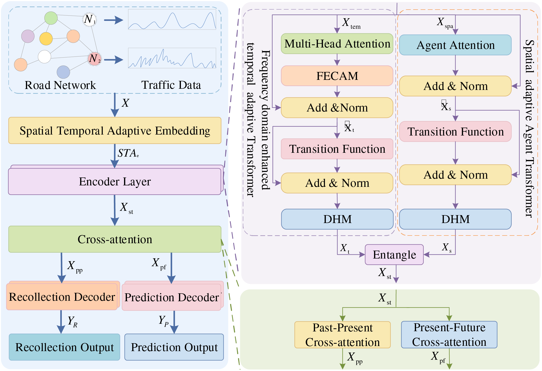
Figure 1: Structure of Bi-STAT+

Bi-STAT+ accepts road network spatial topology and traffic flow data as inputs, denoted by X. First, the STAE module learns efficient feature representations from the input, producing representative spatio-temporal features STAe. The encoder then jointly models spatial topology and temporal sequences, capturing complex dependencies in traffic flows to generate Xst. Based on this, the cross-attention module establishes an efficient information exchange between the encoder and decoder, comprising past–present and present–future cross-attention branches. The past–present branch outputs Xpp, enabling the decoder to fully exploit historical information and mitigate error accumulation. The present–future branch outputs Xpf, assisting in accurate future traffic prediction. Finally, the model is trained using a dual-branch structure comprising a prediction decoder and a recall decoder. The prediction decoder focuses on future traffic flow, outputting YP. The recall decoder reconstructs historical information to reduce overfitting, outputting YR. This design enhances robustness and predictive accuracy, ultimately enabling high-precision traffic flow forecasts.

Overall, compared with the original Bi-STAT, Bi-STAT+ replaces the original Temporal Adaptive Transformer with FDETAT, enhancing the modeling of multiscale temporal features. Instead of the original Spatial Adaptive Transformer, it employs SAAT to dynamically capture local and global interactions among road network nodes, improving the efficiency of spatial dependency modeling.

3.2 Spatio-Temporal Adaptive Embedding

The STAE module takes temporal data and road network structural data as input, and generates a unified feature representation for the model. As shown in Fig. 2, the module is composed of spatial embedding, adaptive reconciliation, and temporal embedding. The implementation details are provided in Algorithm 1.

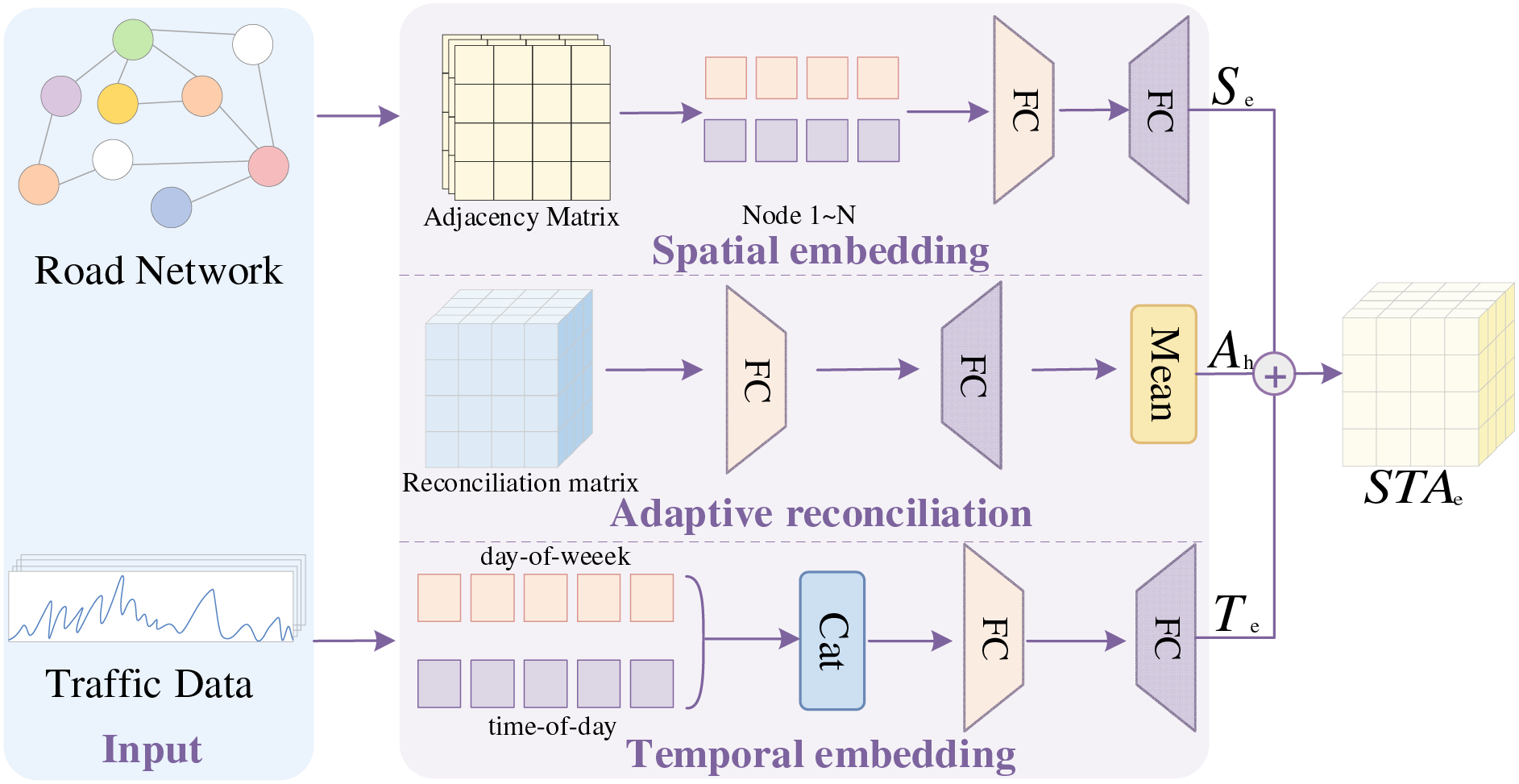
Figure 2: Spatio-temporal adaptive embedding module

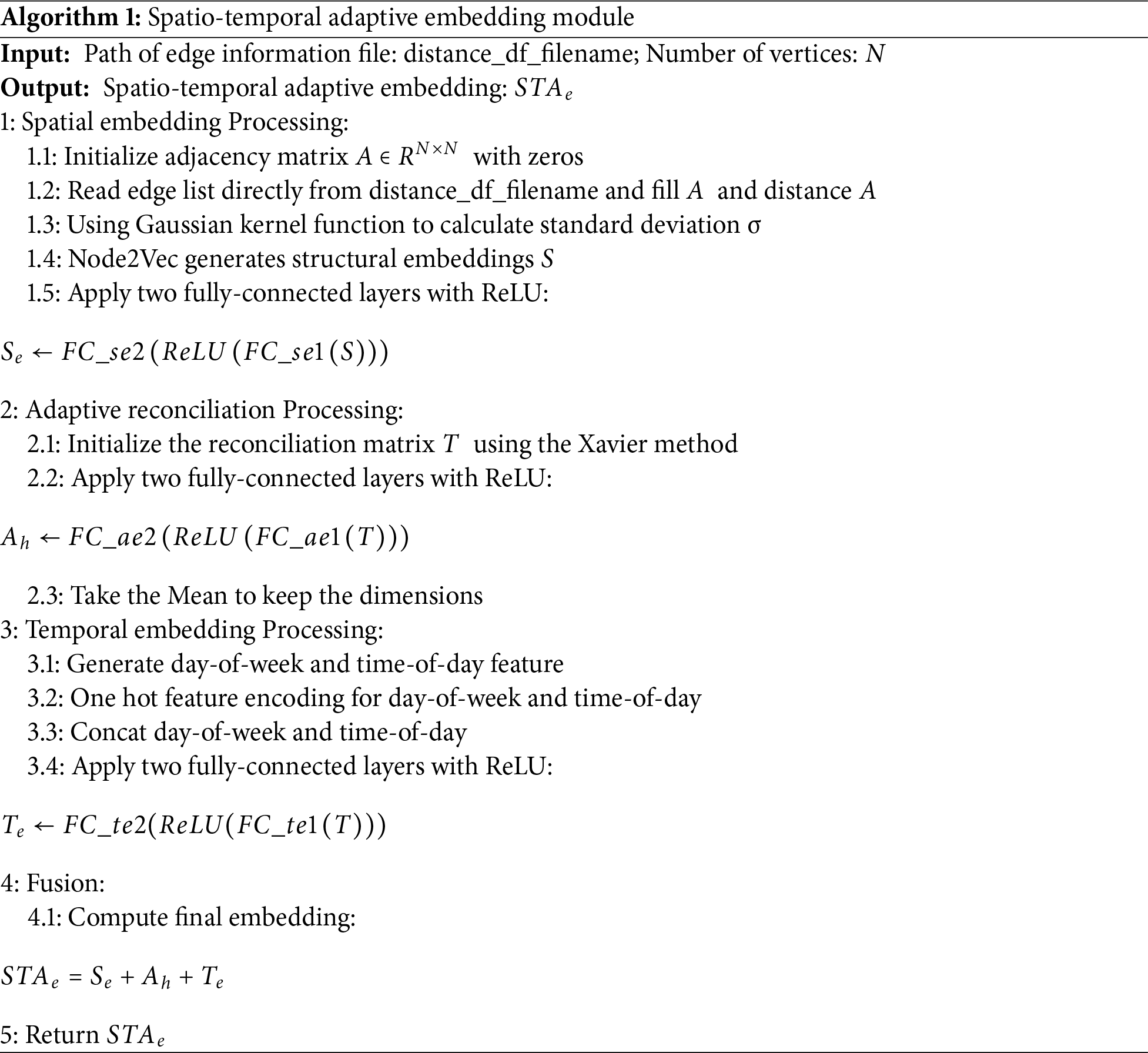
The spatial embedding branch captures spatial characteristics of the road network to model complex spatial dependencies among traffic sensors. A traffic network graph is constructed from actual road network data, where nodes denote traffic sensors and edges indicate road connectivity. Pairwise distances between all traffic sensors are then computed to better reflect actual traffic flow propagation paths. These distances are normalized using a Gaussian kernel function [23] to generate an adjacency matrix that captures spatial correlations between sensors. The node2vec method [24] maps graph nodes (traffic sensors) into low-dimensional feature representations for spatial embedding. These embeddings are then processed through two fully connected layers to align them with the target output dimension, yielding the spatial embedding Se.

The adaptive reconciliation branch does not process input data directly but provides a dynamically adjustable embedding mechanism to enhance the extraction of complex spatio-temporal features. It optimizes embeddings based on data variations by training a reconciliation matrix, improving adaptation to spatio-temporal dependencies in diverse scenarios. Specifically, a learnable parameter tensor of shape (time length, number of nodes, adaptive embedding dimension) is created as the reconciliation matrix and initialized using the Xavier method [25]. The reconciliation matrix is then transformed through two fully connected layers to adjust its dimension and map it to the target output dimension. Finally, the Mean module averages the feature tensors—output from the fully connected layers—over spatial dimensions (different locations) and temporal dimensions (historical, current, and future steps), yielding the adaptive reconciliation representation Ah with consistent dimensions.

The temporal embedding branch captures periodic patterns in traffic data to model recurring traffic flow behaviors. For each time step, two period embedding matrices are generated: day-of-week and time-of-day. These matrices represent weekly and daily periodic features, respectively. They are concatenated to form a comprehensive periodic feature matrix, integrating information across multiple time scales. The concatenated matrix is then fed into two fully connected layers. After a nonlinear transformation, the features are mapped to the target output dimension, producing the periodic embedding Te.

The spatial embedding Se, adaptive reconciliation Ah, and temporal embedding Te are summed to produce the fused spatio-temporal embedding STAe. This fusion enables Ah to dynamically adjust Se and Te, learning optimal feature representations from input context during training. This mechanism strengthens spatio-temporal embedding capability, thereby improving predictive performance.

3.3 Frequency Domain Enhanced Temporal Adaptive Transformer

Traffic flow data typically exhibit complex long-term trends alongside short-term fluctuations. However, the original Temporal Adaptive Transformer primarily models overall temporal dynamics, limiting its ability to capture features across multiple time scales. Moreover, traffic data often contain high-frequency noise (e.g., unexpected events, missing data), which distorts short-term trends and degrades overall prediction accuracy, thereby reducing model robustness and stability. To address these limitations, the FDETAT extends the original structure by integrating the Frequency-Enhanced Channel Attention Mechanism (FECAM) [26]. This integration strengthens the model’s ability to capture both long- and short-term traffic flow features via frequency-domain enhancement.

As shown in Fig. 1, the FDETAT comprises five key components: Multi-Head Attention, FECAM, Add & Norm, Transition Function, and DHM. The architecture takes the temporal feature Xtem as input and learns global dependencies through Multi-Head Attention, capturing correlations between different time steps. Subsequently, FECAM extracts both long- and short-term temporal features, enhancing the model’s perception of diverse temporal patterns. A residual connection followed by normalization transforms the temporal features into optimized representations, denoted as X^t. The Transition Function module then adjusts the feature space to maximize information flow, enabling efficient transformations between temporal features. Finally, the DHM component selectively halts or continues information delivery, prioritizing task-relevant data. This module improves information-processing efficiency and allows dynamic adjustment of computational steps based on task complexity. Ultimately, the optimized temporal features Xt are used in subsequent decoding stages to enhance task-specific performance.

As the core of FDETAT, FECAM processes traffic flow data in the frequency domain using the Discrete Cosine Transform (DCT) [27]. Through this transform, FECAM models temporal characteristics at multiple frequency scales, enhancing the model’s ability to capture complex spatio-temporal patterns. Low-frequency components reveal long-term trends and periodic patterns (e.g., day–night cycles, peak hours), whereas high-frequency components capture short-term fluctuations and localized changes (e.g., traffic accidents, missing data from sensor failures). FECAM compensates for the limitations of traditional multi-attention mechanisms in frequency-domain information extraction, thereby improving adaptability and robustness in complex traffic scenarios.

The overall architecture of FECAM is illustrated in Fig. 3. The input to FECAM is the traffic flow feature T, comprising time series data for N nodes, each of length L, representing traffic flow observations at discrete time points. Specifically, T is split along the node dimension into N subsequences {v0,v1,…,vN−1}, where each vi denotes the time series of a single traffic node. Each vi is transformed using the DCT to obtain its frequency representation Freqi. The DCT maps time-domain data to the frequency domain, enabling the model to capture cyclical patterns—information crucial for modeling periodic trends in traffic flow. The frequency representations {Freq0,Freq1,…,FreqN−1} from all nodes are stacked to form the complete frequency-domain tensor Freq, preserving frequency information across nodes. This tensor Freq passes through a fully connected layer to learn task-specific frequency-domain features, followed by normalization to produce an importance weight matrix that quantifies the contribution of each frequency component to prediction. The computed importance weights are applied element-wise to T, amplifying beneficial frequency components while suppressing irrelevant or noisy ones. The computational procedure of FECAM is formally defined in Eq. (1):

T′=T×(Norm(FC(Stack(DCT(Split(T))))))(1)

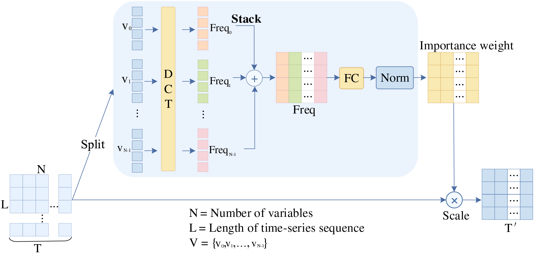
Figure 3: FECAM module

By incorporating attention in the frequency domain, FECAM focuses on critical frequency components in time-series data, thereby improving traffic flow prediction and enhancing the capture of both periodic and trending patterns.

3.4 Spatial Adaptive Agent Transformer

Spatial relationships in traffic flow data typically show strong localization, where traffic in a given road segment is mainly influenced by its neighboring segments, and correlations diminish as spatial distance increases. In traditional spatial adaptive transformers, the multi-head attention mechanism assigns weights to all nodes to capture global relationships. However, this global allocation can cause weight dispersion, reducing the ability to effectively capture critical local interactions.

As illustrated in Fig. 1, the SAAT model replaces conventional multi-head attention with the Agent Attention mechanism [28]. The module receives the spatial feature matrix Xspa as input, applies Agent Attention to adaptively learn the importance of different regions, and dynamically reallocates computational resources, thereby improving its ability to capture both local and global dependencies. After residual concatenation and normalization, the spatial features are transformed into optimized representations X^s. A transition module then adjusts the feature representation space to optimize information transfer and ensure effective mapping between spatial dimensions. Finally, the DHM component selectively halts or continues information transfer, enabling the model to dynamically focus on key features relevant to the current task. The resulting optimized spatial feature Xs serves as the final representation for subsequent decoding stages, enhancing performance, particularly in complex spatio-temporal dependency scenarios.

In Agent attention, the traditional attention triplet (Q,K,V) is extended to a quadruplet (Q,A,K,V), introducing an additional agent vector A for aggregating information from K and V, and then transferring to Q to model global information. The overall structure of Agent Attention comprises two standard Softmax Attention operations and is mathematically equivalent to a generalized linear attention mechanism. In this way, Agent attention seamlessly integrates high-performance Softmax Attention with efficient linear attention, maintaining sensitivity to local influences while preserving a global understanding of the entire transportation network.

Fig. 4 depicts the detailed workflow of the Agent attention module. The process begins with a linear transformation of the input traffic network adjacency matrix S, generating the query (Q), key (K), and value (V) matrices for subsequent attention computation. The query matrix Q then undergoes pooling to extract Agent Tokens (A), which aggregate features from multiple sensor nodes. In the first stage, Agent Features are computed as shown in Eq. (2). The Agent Tokens A serve as new queries in a Softmax Attention operation with the key matrix K, producing Agent Features Oagent that enhance the model’s perception of critical traffic patterns.

Oagent=softmax(AKTd+B1)⋅V(2)

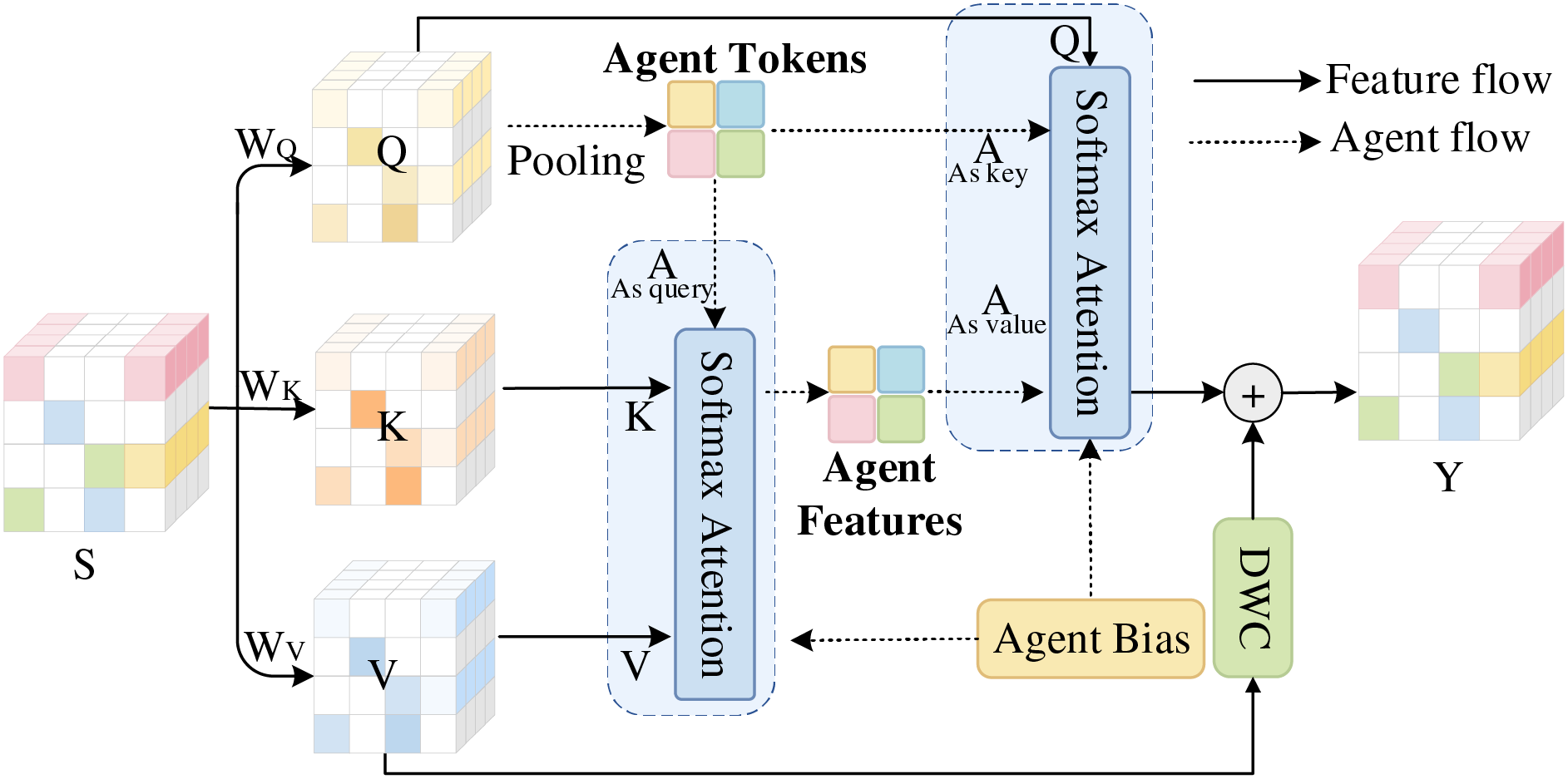
Figure 4: Agent attention module

Next, perform a Softmax Attention operation taking Oagent as value and A as key, and keeping the original Q as query, which strengthens global feature interactions and yields the intermediate feature O, as Eq. (3) shows.

O=softmax(Q(A)Td+B2)⋅Oagent(3)

The final output Y directly fused the intermediate feature O and local feature which is processed by Depthwise Separable Convolution (DWC), as shown in Eq. (4).

Y=O+DWC(V)(4)

This workflow combines a two-stage Softmax Attention mechanism with a local fusion stage via deep convolution, enabling the model to capture both global context and local traffic dynamics.

4  Experiments

4.1 Datasets and Preprocessing

This study employed four real-world traffic flow datasets for model validation, comprising two public and two private datasets. The public datasets are the widely used traffic flow prediction benchmarks PeMS04 and PeMS08 [29]. The private datasets, obtained from traffic surveillance systems in Chengdu and Baotou, China, encompass diverse traffic scenarios and complex environmental conditions, thereby enhancing the comprehensiveness and generalizability of model validation. Detailed dataset descriptions are provided in Table 1, while Fig. 5a,b illustrates the spatial distribution of sensors in the two private datasets.

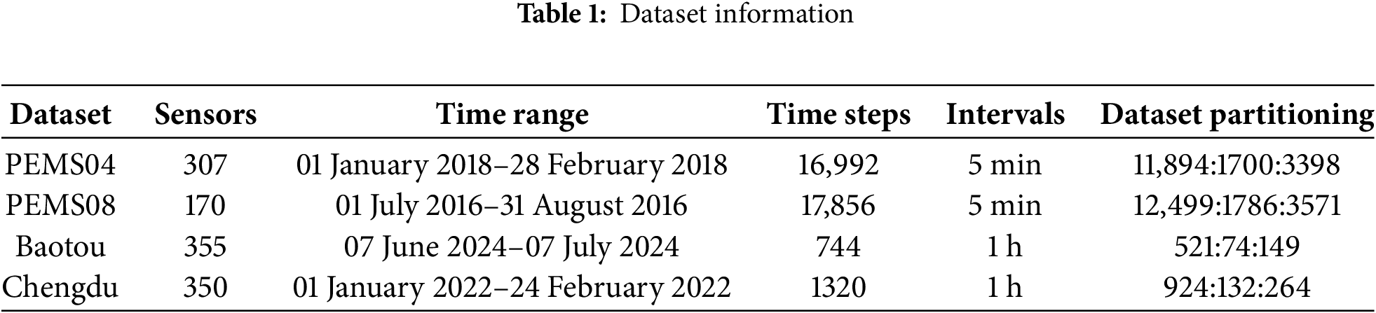
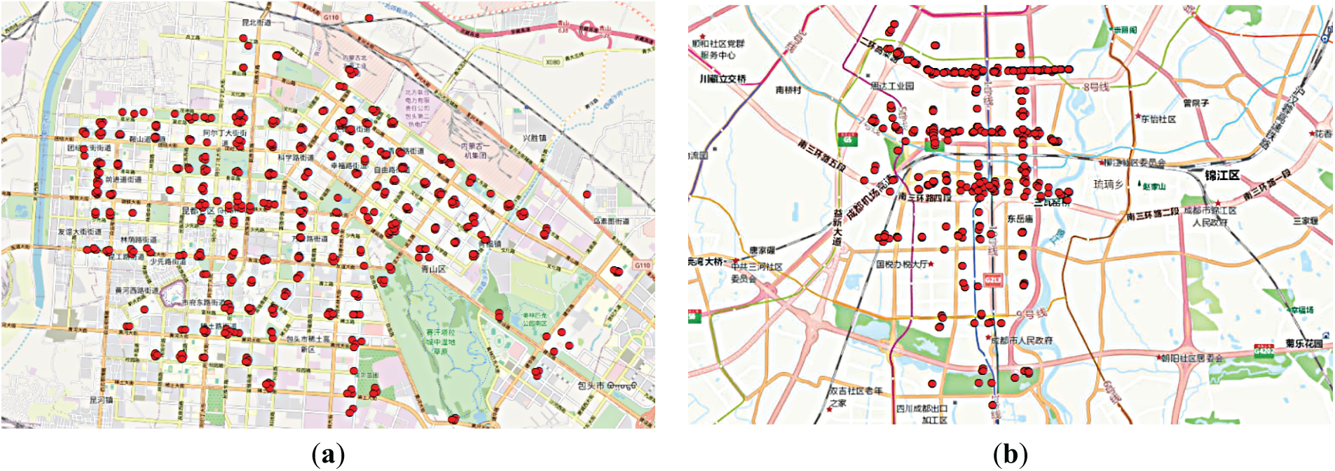
Figure 5: (a) Distribution of nodes in Baotou; (b) Distribution of nodes in Chengdu

During data preprocessing, a comprehensive data cleaning and processing scheme was developed. First, based on integrity analysis, the original monitoring data were screened. Data from monitoring points with high missing rates, along with their corresponding periods, were removed to ensure reliability. Second, for the filtered dataset, missing values were filled using linear interpolation. This method preserves temporal continuity and ensures spatial consistency. To ensure experimental rigor, a stratified sampling strategy was applied, dividing all datasets into training, validation, and test sets in a 7:1:2 ratio based on temporal order (see Table 1 for details). The division strictly followed temporal continuity, ensuring no overlap in time between subsets. This approach effectively prevented data leakage and provided a robust foundation for subsequent model training and evaluation.

4.2 Baselines

To thoroughly assess the predictive performance of the Bi-STAT+ model, 14 representative benchmark models were selected for comparative experiments. These comprise one traditional statistical model, HA (1997) [30]; five deep learning models based on Graph Neural Networks (GNNs)—ASTGCN (2019) [8], AGCRN (2020) [7], STFGNN (2021) [31], DSTAGNN (2022) [32], and ST-CGCN (2023) [10]; and eight deep learning models based on the Transformer architecture—GMAN (2020) [14], ASTGNN (2021) [33], Traffic Transformer (2022) [13], Bi-STAT (2022) [15], MFE-STL (2024) [34], STFGCN (2024) [11], GAMAN (2025) [35], and FDGT (2025) [36].

4.3 Experimental Setups

The experimental platform runs on Ubuntu 20.04 LTS, with model implementation based on the PyTorch 2.1.1 deep learning framework. The hardware configuration comprises an Intel® Xeon® E5-2667 v3 processor (3.20 GHz), 24 GB RAM, and an NVIDIA GeForce RTX 3090 GPU (CUDA 12.2).

Following experimental validation and parameter tuning, the model training parameters were configured as follows. The batch size was set to 4 for the PeMS04 and PeMS08 datasets, and to 2 for the larger Baotou and Chengdu datasets. The encoder–decoder depth was set to two layers for all datasets, except for PeMS04, where a single layer was used due to its data characteristics. The Adam optimizer was employed with an initial learning rate of 0.001, combined with a ReduceLROnPlateau scheduler for dynamic adjustment. Training was conducted for 100 epochs, with early stopping triggered if validation performance failed to improve for 10 consecutive epochs. The DHM penalty term weight and recall decoder weight were both set to 0.001, and the reconciliation matrix dimension was fixed at 80.

4.4 Evaluation Metrics

To assess model prediction performance, three widely used evaluation metrics are employed: mean absolute error (MAE), root mean square error (RMSE), and mean absolute percentage error (MAPE). All three metrics quantify the deviation between predicted and actual values, with smaller values indicating higher prediction accuracy and larger values indicating greater prediction error. The formulas for each metric are provided in Eqs. (5)–(7).

MAE=1n∑i=1n|yi−y^i|(5)

RMSE=1n∑i=1n(yi−y^i)2(6)

MAPE=1n∑i=1n|yi−y^iyi|×100%(7)

4.5 Comparison with the SOTA Methods

4.5.1 Comparative Experiments on Public Datasets

This section evaluates the predictive performance of the proposed Bi-STAT+ model against multiple benchmark models on the PEMS04 and PEMS08 datasets. In all experiments, the historical step size (H), current step size (P), and forecast step size (F) were set to 12. For datasets in the PEMS series, with a time granularity of 5 min, the model uses the most recent 1 h of historical data to forecast traffic flow for the next hour. The results are summarized in Table 2, where bold values indicate the best performance and underlined values denote the second best. All results are reported as the mean values over 12-step forecasts.

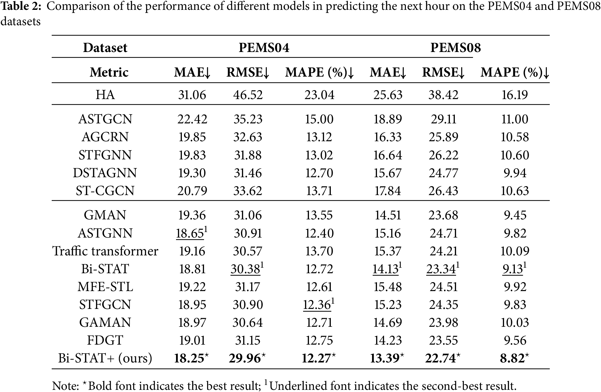
On both PEMS04 and PEMS08, model performance varies markedly. Bi-STAT+ achieves the highest accuracy, whereas the traditional HA model performs the worst. For PEMS04, Bi-STAT+ reduces MAE by about 4% compared with the latest Transformer-based model, FDGT. For PEMS08, Bi-STAT+ achieves reductions of approximately 5.2%, 2.6%, and 3.4% in the respective metrics compared with the second-best model, Bi-STAT.

The observed performance differences stem from each model’s ability to capture spatio-temporal traffic dynamics. HA relies solely on historical averages and ignores dynamic patterns, resulting in the poorest performance. Graph neural network-based models (e.g., ASTGNN) can capture spatial correlations but struggle with temporal precision and depend partly on fixed network topologies, limiting adaptability to dynamic changes. Transformer-based models (e.g., FDGT) excel in modeling long-range dependencies, yet their fixed time-window attention cannot adjust to varying traffic patterns, leading to noise accumulation. In contrast, Bi-STAT+ employs a FDETAT to separately model high-frequency fluctuations and low-frequency trends. Combined with dynamic graph structure optimization, it achieves a deep integration of spatial and temporal features, yielding superior performance.

To further evaluate the models’ advantages in traffic flow prediction, additional experiments were conducted on PEMS04 and PEMS08 with varying prediction horizons. Four forecast intervals were considered: short-term (1 step/5 min), medium-term (3 steps/15 min), medium-to-long-term (6 steps/30 min), and long-term (12 steps/60 min), enabling a comprehensive evaluation across time scales. Quantitative results for each model are presented in Tables 3 and 4, while Fig. 6 illustrates the performance trends across different prediction horizons using line charts.

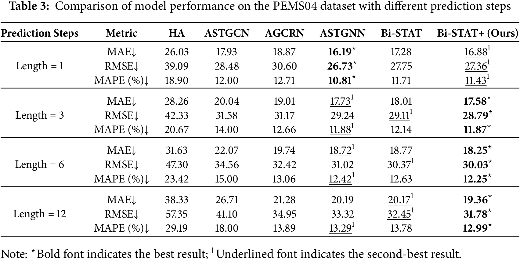
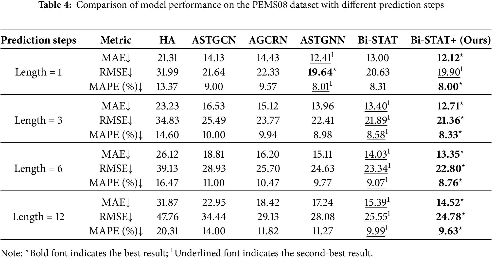
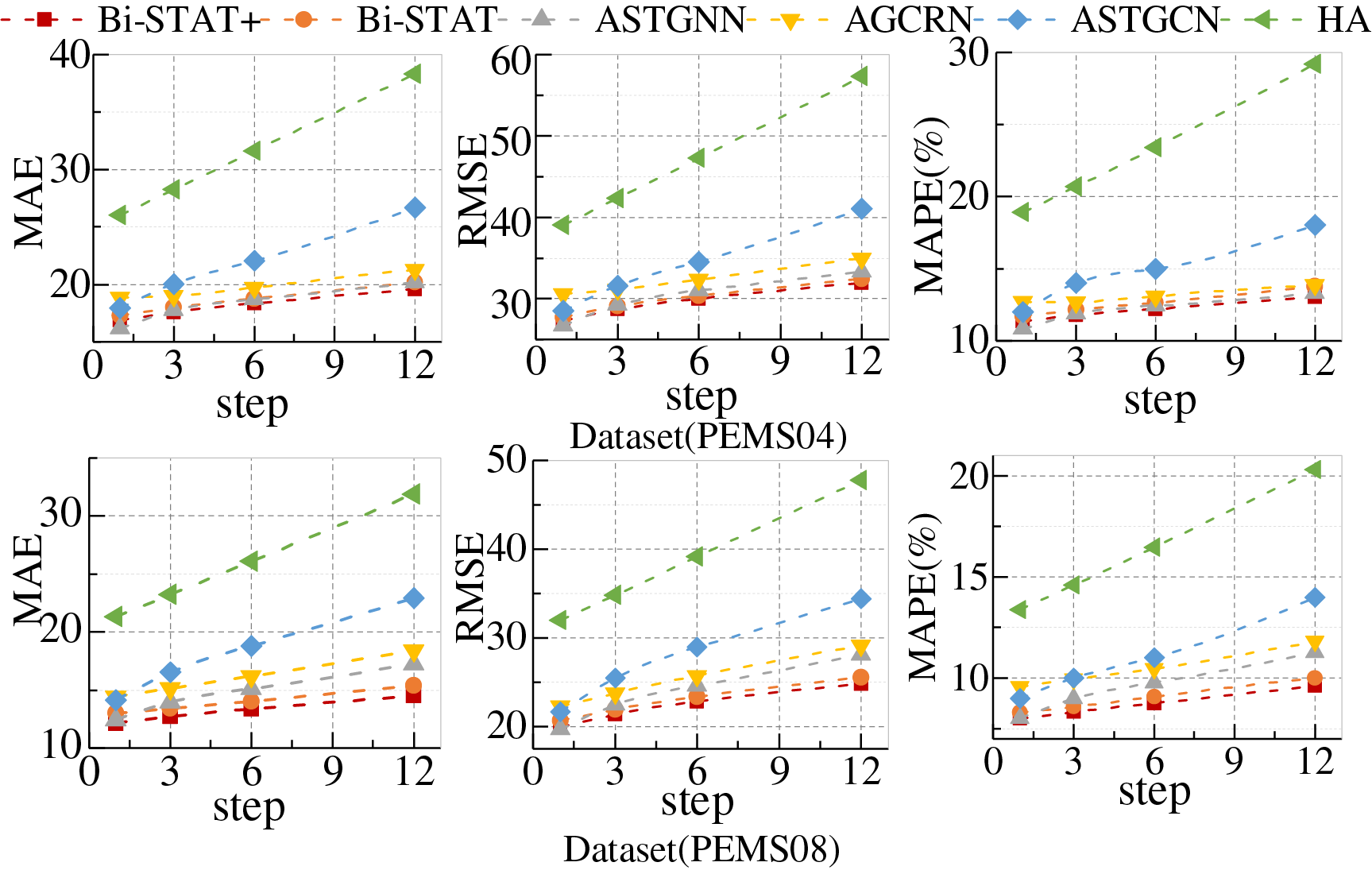
Figure 6: Predictive performance of PEMS dataset at different step sizes

Across different prediction horizons, model performance varies notably. Bi-STAT+ achieves the best overall results, with its advantage becoming more pronounced at longer horizons. On PEMS04, ASTGNN slightly outperforms Bi-STAT+ for short-term (1-step) predictions, while Bi-STAT+ leads in medium- to long-term forecasts (3-step, 6-step, 12-step). On PEMS08, Bi-STAT+ consistently ranks first across all horizons, with 12-step errors reduced by 0.87, 0.77, and 0.36 in the respective metrics compared with Bi-STAT. Although errors for all models increase with the prediction horizon, the growth is smallest for Bi-STAT+.

The performance differences across prediction horizons stem from each model’s capacity to capture features at different time scales. Short-term (1-step) forecasts are heavily influenced by instantaneous factors. ASTGNN’s dynamic graph structure effectively captures local spatial correlations, whereas Bi-STAT+’s trend-smoothing mechanism responds slightly slower to sudden fluctuations. Long-term (12-step) forecasts depend on periodic patterns. The FDETAT module in Bi-STAT+ decomposes and accurately models low-frequency trends, thereby mitigating noise accumulation.

4.5.2 Comparative Experiments on Private Datasets

To assess the generalization capability of the proposed model, we compare the predictive performance of Bi-STAT+ with multiple benchmark models on private datasets from Baotou and Chengdu. In all experiments, the historical step size (H), current step size (P), and prediction step size (F) are set to 12. For both datasets, which have a time granularity of 1 h, the model uses the most recent 12 h of traffic data to forecast the next 12 h. Detailed results are provided in Table 5, with all values representing the mean of 12-step forecasts.

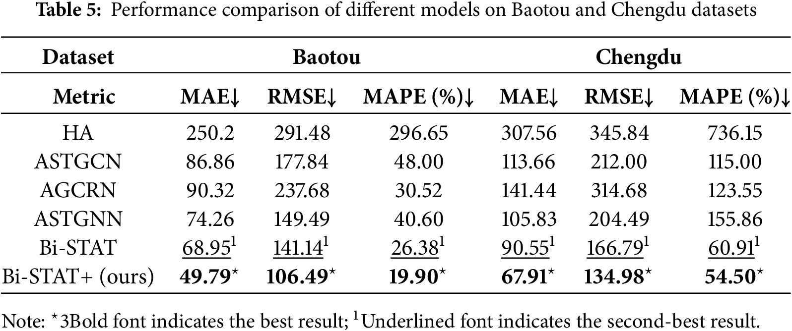
As shown in Table 5, Bi-STAT+ achieves the best performance across all evaluation metrics for both Baotou and Chengdu. These results indicate that Bi-STAT+ maintains stable and high predictive accuracy despite the spatio-temporal variations in traffic patterns between cities, thereby demonstrating strong generalization capability.

Similar to the experiments on the public datasets, we also conducted comparative experiments with varying prediction horizons on the Baotou and Chengdu private datasets. The quantitative results for each model are presented in Tables 6 and 7, while Fig. 7 provides a line chart illustrating how prediction performance changes with the forecast horizon.

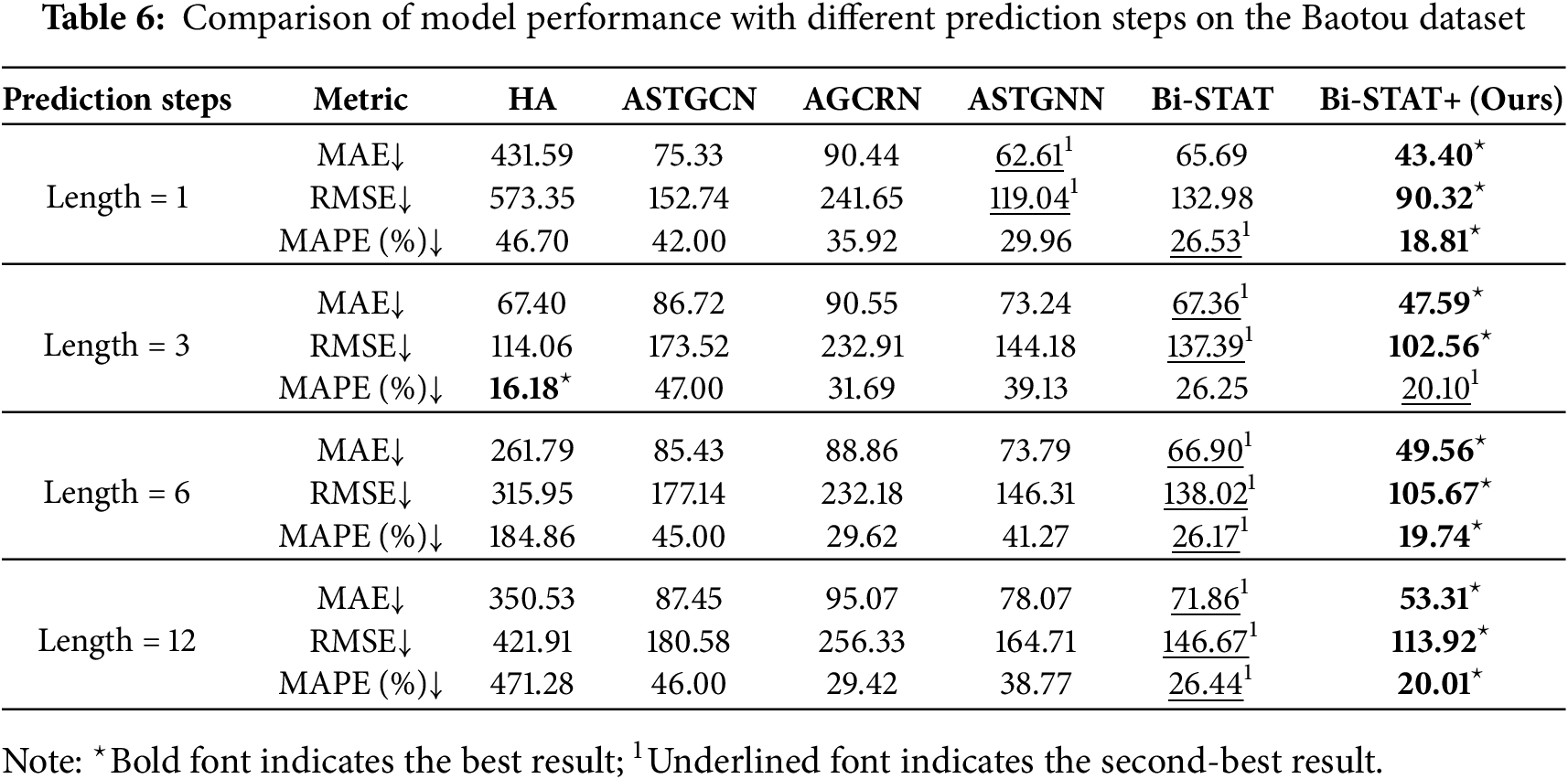
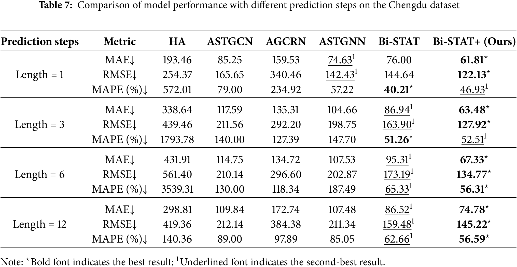
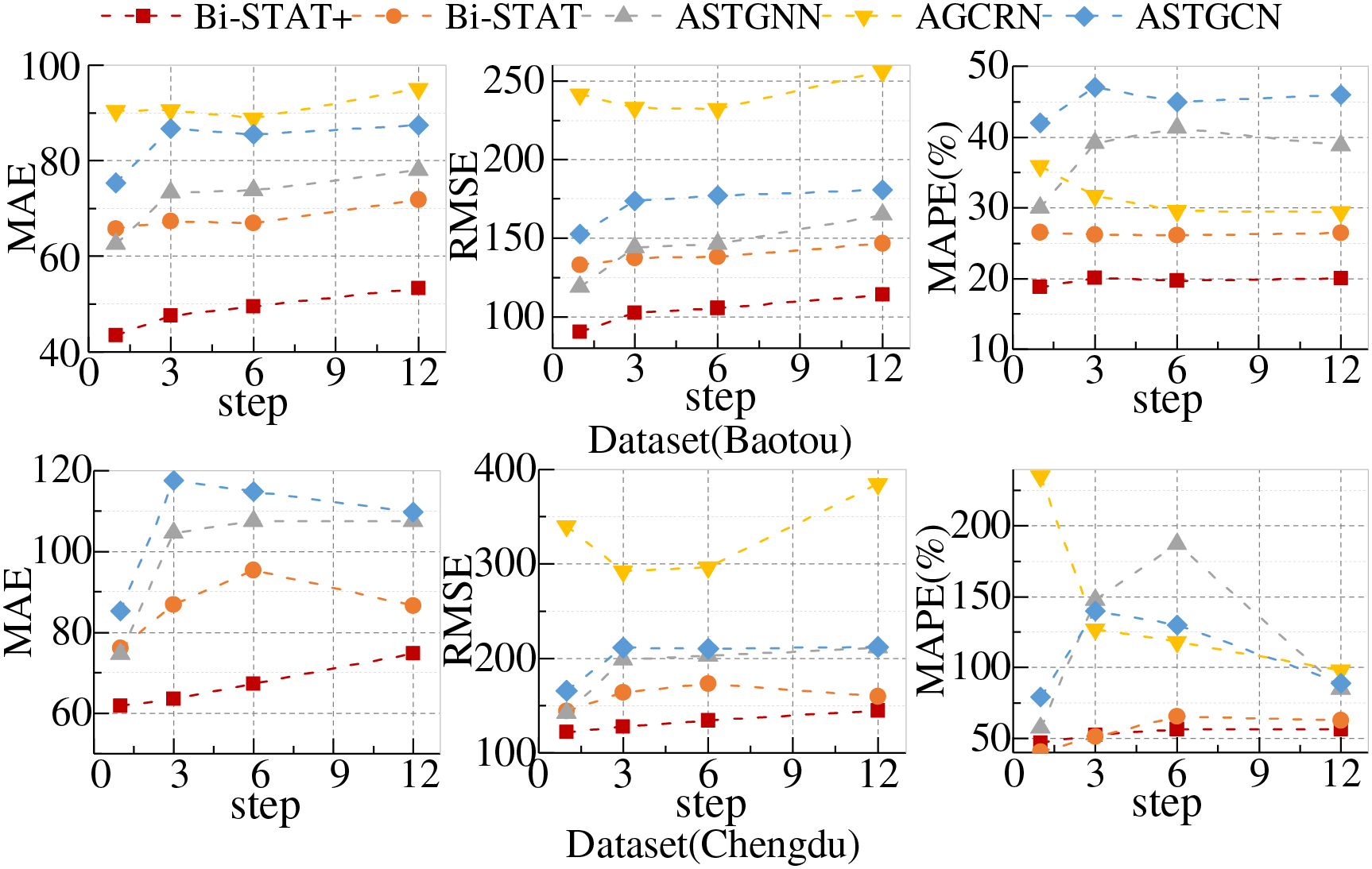
Figure 7: Predictive performance of Baotou and Chengdu datasets at different step sizes

4.6 Ablation Study

This study conducts ablation experiments on four datasets to evaluate the contribution of each core innovation in the Bi-STAT+ model to traffic flow prediction. Four variant models are designed to analyze the specific effects of individual components.

Variant Model 1: Removes the FECAM module and replaces the Agent Attention Mechanism with multi-head attention to evaluate the combined contribution of FECAM and Agent Attention to overall performance.

Variant Model 2: Removes the FECAM module from FDETAT, which reduces the model’s ability to capture temporal contextual information.

Variant Model 3: Replaces the Agent Attention Mechanism in SAAT with multi-head attention, thereby reducing the model’s ability to adaptively allocate attention across nodes.

Variant Model 4: Removes the Adaptive Reconciliation Embedding (AAE) module, reducing the model’s ability to embed dynamic temporal and spatial information.

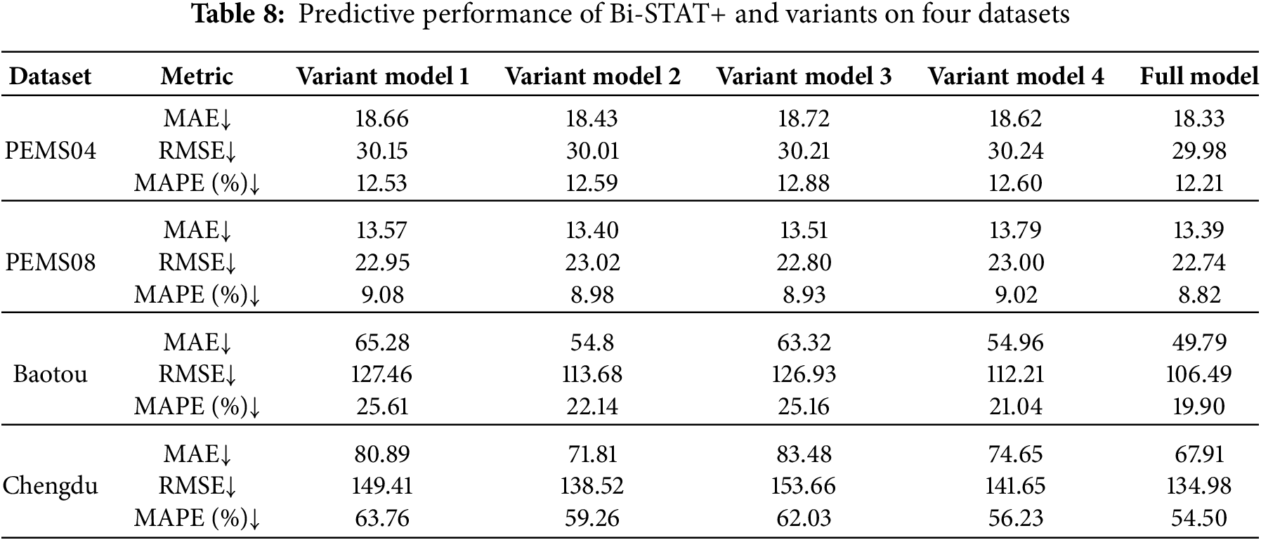
Table 8 summarizes the performance of Bi-STAT+ and its variants across the four datasets, followed by the corresponding analysis.

1.    Contribution of the FECAM Module: Removing the FECAM module led to a notable performance decline, particularly on the Baotou dataset, where the MAE rose from 49.79 to 54.80. This demonstrates that the FECAM module leverages frequency-domain analysis to jointly model high-frequency details and low-frequency trends, thereby improving the representation of multi-scale temporal features.

2.    Effectiveness of the Agent Attention Mechanism: Replacing the Agent Attention Mechanism with traditional multi-head attention resulted in a clear drop in prediction accuracy across all four datasets. For example, on the PEMS04 dataset, the MAE increased from 18.33 to 18.72. This finding indicates that the Agent Attention Mechanism adaptively allocates attention weights to traffic sensors at different locations based on dynamic traffic network changes, enabling better capture of both local and global spatial features. Its advantage is particularly evident on the PEMS04 dataset, which features a large number of nodes and a complex topology.

3.    Importance of the AAE Module: Removing the AAE module also reduced performance. On the PEMS04 dataset, the MAE increased from 18.33 to 18.62. The AAE module strengthens spatio-temporal feature embedding through adaptive reconciliation matrices, allowing Bi-STAT+ to better capture dynamic spatio-temporal dependencies and thereby enhance prediction accuracy.

4.7 Robustness Analysis

In real-world traffic flow data collection, sensor measurements are frequently affected by factors such as poor contact and natural aging, resulting in noise interference. Environmental conditions and limited sensor lifespans make it difficult to fully eliminate noise caused by aging. Such interference can significantly reduce the accuracy of traffic flow prediction models.

To evaluate the robustness of Bi-STAT+ in noisy environments, we compare its performance with several benchmark models on the Baotou dataset. Data loss is simulated by randomly removing 20%, 40%, and 60% of the records. Gaussian noise with a mean of 10 and a standard deviation of 500 is then added at the same proportions to mimic real-world uncertainties, including measurement errors and outliers. Tables 9 and 10 summarize the prediction performance of Bi-STAT+ and the benchmark models under different levels of missing data and noise.

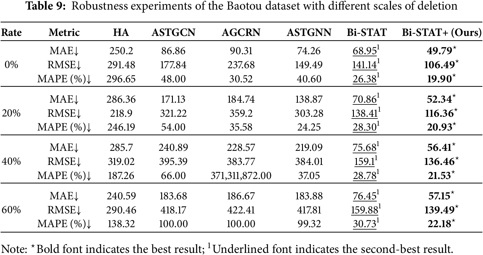
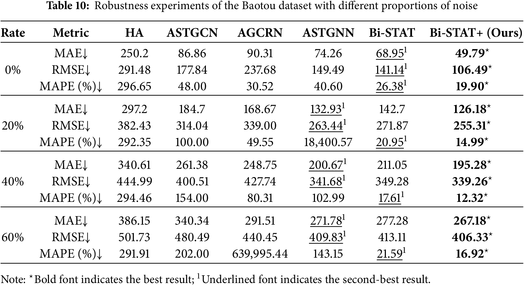
The results show that Bi-STAT+ exhibits greater robustness than the benchmark models under missing data and noise conditions. With 20% missing data and noise, the MAE of Bi-STAT+ rises only slightly, while other graph-based models suffer more substantial degradation. Even as missing data and noise levels reach 40% and 60%, Bi-STAT+ maintains relatively stable accuracy, with only moderate increases in MAE. Under severe noise interference, it effectively suppresses the impact of Gaussian noise, demonstrating strong noise tolerance.

4.8 Sampling Frequency Analysis

As shown in Section 4.5, prediction errors on private datasets are notably higher than on public datasets, mainly due to differences in data collection frequency. The PEMS dataset employs a 5-min sampling interval, which yields strong correlations between consecutive time steps. Consequently, a 12-step prediction covers only the next hour, thereby facilitating the capture of short-term dynamics. In contrast, private datasets are sampled hourly, greatly weakening temporal correlations. A 12-step prediction must then span 12 h of traffic flow changes, thereby amplifying cumulative errors and increasing the difficulty of the prediction.

To examine the effect of sampling frequency on prediction accuracy, we performed resampling experiments on the Baotou and Chengdu datasets. The original traffic data were resampled to 30-min, 15, 10, and 5-min intervals. Two preprocessing steps were applied: (1) linear interpolation filled in missing time steps during resampling; and (2) a moving-average method smoothed the prediction values for the final time step. Tables 11 and 12 present the prediction errors of Bi-STAT+ and the benchmark models under different sampling frequencies.

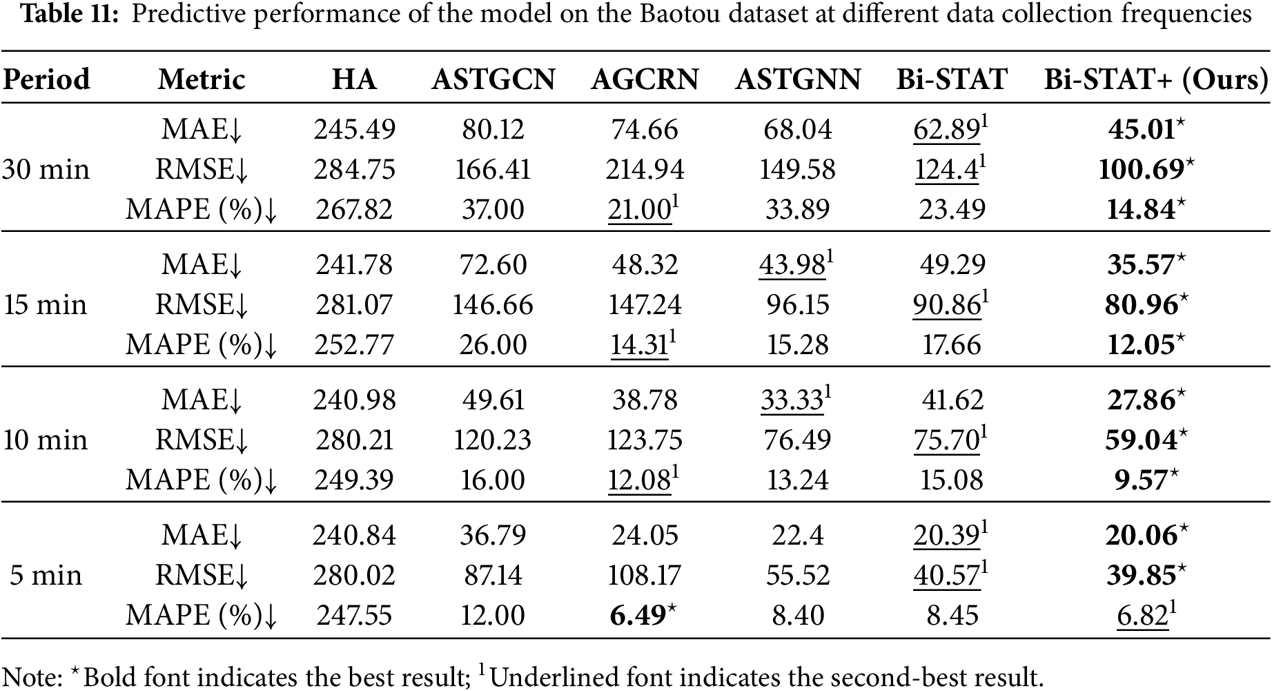
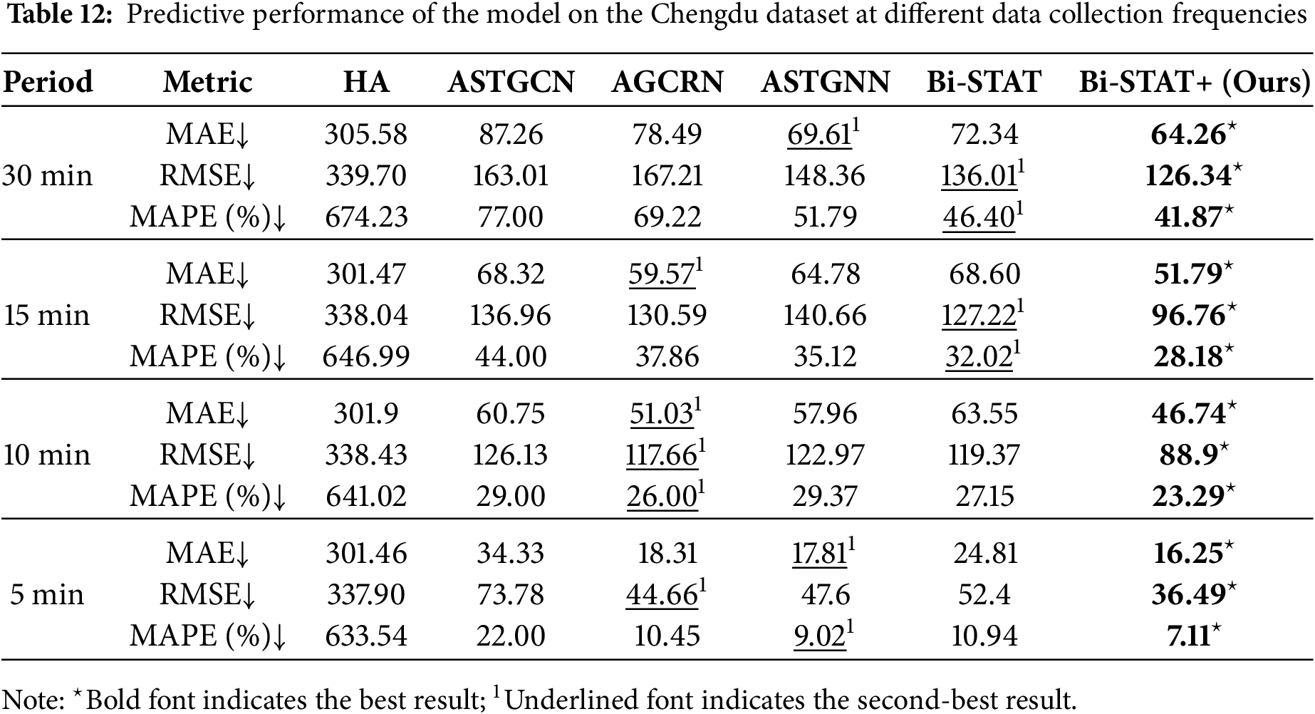
Experimental results show that as the sampling interval decreases from 1 h to 5 min, the prediction errors of both Bi-STAT+ and the benchmark model decline markedly. This supports our hypothesis that longer intervals increase prediction uncertainty and error. Shorter intervals strengthen temporal correlations, allowing the model to capture traffic flow dynamics more accurately and thereby reduce prediction errors.

4.9 Visual Result Analysis

Using the 5-min sampling frequency traffic flow dataset from Baotou City, two sensor nodes with distinct location characteristics—No. 98 (residential area) and No. 205 (commercial area)—were selected for analysis, with their spatial positions shown in Fig. 8a,b. Traffic flow prediction performance was evaluated for different forecast horizons (15, 30, and 60 min) on 07 July 2024 (Sunday). As shown in Fig. 9a–f, the Bi-STAT+ predictions (red dashed line) closely align with the actual traffic flow (blue solid line) over time. Across both short-term (15 min) and long-term (60 min) forecasts, Bi-STAT+ maintains high accuracy and stability across different nodes. Notably, during peak traffic periods, it captures rapid fluctuations in traffic speed and accurately reflects dynamic changes in traffic volume. Moreover, performance variations between nodes in different locations suggest that Bi-STAT+ offers advantages in handling geospatial heterogeneity.

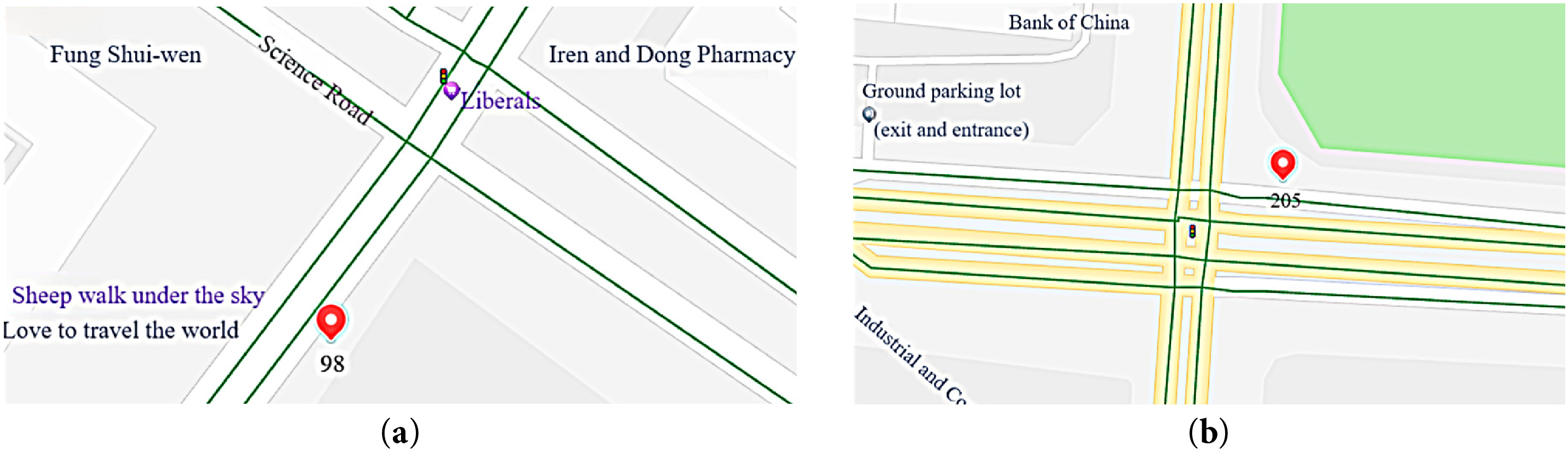
Figure 8: (a) Node 98 (red marker); (b) Node 205 (red marker)

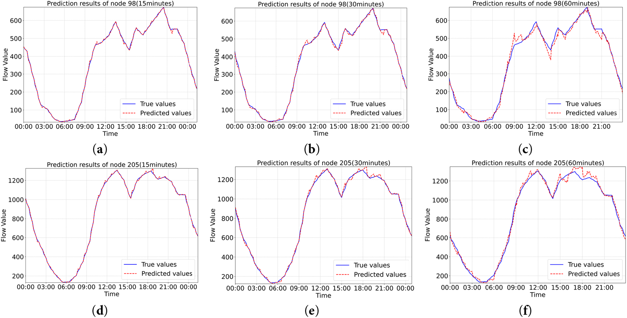
Figure 9: (a) Plot of sensor node #98 at 15 min of prediction; (b) Plot of sensor node #98 at 30 min of prediction; (c) Plot of sensor node #98 at 60 min of prediction; (d) Plot of sensor node #205 at 15 min of prediction; (e) Plot of sensor node #205 at 30 min of prediction; (f) Plot of sensor node #205 at 60 min of prediction. (blue straight line is true value, red dashed line is predicted value)

4.10 Real-Time Applicability Evaluation

To validate the real-time capability of Bi-STAT+, we measured its inference speed on traffic networks from Baotou and Chengdu under identical experimental settings (Section 4.3). Results show that Bi-STAT+ processes full-network predictions in 0.97 s (Baotou) and 3.88 s (Chengdu), while the baseline Bi-STAT requires 0.15 and 1.52 s, respectively. Although Bi-STAT+ incurs higher computational costs due to its enhanced architecture, both models operate well within the 5 s real-time threshold for traffic management systems. This efficiency ensures practical deployment in smart city applications without sacrificing prediction quality.

5  Conclusions

This study presents Bi-STAT+, an advanced spatio-temporal transformer framework that significantly advances urban traffic flow forecasting. The proposed model integrates dynamic adaptive encoding via STAE with enhanced attention mechanisms (FDETAT/SAAT), demonstrating superior capability in capturing complex spatio-temporal dependencies. Extensive experimental evaluations on real-world datasets validate the framework’s effectiveness, showing consistent improvements of 15.6% in prediction accuracy and 11.6% in robustness compared to SOTA methods. The systematic analysis of sampling frequency effects provides valuable insights for practical implementation. These contributions not only establish a new benchmark in traffic forecasting research but also offer significant potential for real-world applications in intelligent transportation systems and smart city development.

Future research will proceed in two directions. First, we aim to further improve the model’s computational efficiency. Although the current version meets real-time application requirements, ongoing urbanization and rising vehicle ownership continue to increase the complexity and scale of traffic data. This creates opportunities to optimize the model’s architecture and reduce inference time to meet stricter performance demands. Second, we will address the challenge of predicting traffic flow at checkpoints lacking historical data. By integrating external information such as road network topology and POI distribution, we plan to develop an adaptive framework that leverages data from adjacent checkpoints to estimate traffic flow at newly deployed nodes, thereby broadening the model’s applicability.

Acknowledgement: Not applicable.

Funding Statement: This work was partly supported by the Youth Foundation of the Inner Mongolia Natural Science Foundation [grant number 2024QN06017 and 2025MS06022], the Basic Scientific Research Business Fee Project for Universities in Inner Mongolia [grant numbers 2023XKJX019 and 2023XKJX024], the Central Guidance on Local Science and Technology Development Fund through [grant number 2024ZY0084].

Author Contributions: Conceptualization, Yali Cao and Weijian Hu; methodology, Yali Cao; software, Yali Cao; validation, Yali Cao, Weijian Hu and Lingfang Li; formal analysis, Yali Cao; investigation, Yali Cao; resources, Yali Cao; data curation, Yali Cao; writing—original draft preparation, Yali Cao; writing—review and editing, Yali Cao, Weijian Hu, Lingfang Li, Minchao Li, Meng Xu and Ke Han; visualization, Yali Cao; supervision, Weijian Hu, Lingfang Li, Minchao Li, Meng Xu and Ke Han; project administration, Yali Cao; funding acquisition, Weijian Hu. All authors reviewed the results and approved the final version of the manuscript.

Availability of Data and Materials: Data available on request from the authors. The data that support the findings of this study are available from the corresponding author, Lingfang Li, upon reasonable request.

Ethics Approval: Not applicable.

Conflicts of Interest: The authors declare no conflicts of interest to report regarding the present study.

References

1. Zhou S, Wei C, Song C, Pan X, Chang W, Yang L. Short-term traffic flow prediction of the smart city using 5G Internet of vehicles based on edge computing. IEEE Trans Intell Transp Syst. 2023;24(2):2229–38. doi:10.1109/TITS.2022.3147845. [Google Scholar] [CrossRef]

2. Chen J, Zheng L, Hu Y, Wang W, Zhang H, Hu X. Traffic flow matrix-based graph neural network with attention mechanism for traffic flow prediction. Inf Fusion. 2024;104(6):102146. doi:10.1016/j.inffus.2023.102146. [Google Scholar] [CrossRef]

3. Zhang C, Patras P. Long-term mobile traffic forecasting using deep spatio-temporal neural networks. In: Proceedings of the Eighteenth ACM International Symposium on Mobile Ad Hoc Networking and Computing; 2018 Jun 26–29; Los Angeles, CA, USA. doi:10.1145/3209582.3209606. [Google Scholar] [CrossRef]

4. Shao Y, Zhao Y, Yu F, Zhu H, Fang J. The traffic flow prediction method using the incremental learning-based CNN-LTSM model: the solution of mobile application. Mob Inf Syst. 2021;2021(4):5579451. doi:10.1155/2021/5579451. [Google Scholar] [CrossRef]

5. Yuan H, Li G, Bao Z, Feng L. An effective joint prediction model for travel demands and traffic flows. In: 2021 IEEE 37th International Conference on Data Engineering (ICDE); 2021 Apr 19–22; Chania, Greece. doi:10.1109/icde51399.2021.00037. [Google Scholar] [CrossRef]

6. Qi X, Hu W, Li B, Han K. STGNN-FAM: a traffic flow prediction model for spatiotemporal graph networks based on fusion of attention mechanisms. J Adv Transp. 2023;2023(2):8880530. doi:10.1155/2023/8880530. [Google Scholar] [CrossRef]

7. Bai L, Yao L, Li C, Wang X, Wang C. Adaptive graph convolutional recurrent network for traffic forecasting. In: Proceedings of the 34th Conference on Neural Information Processing Systems (NeurIPS 2020); 2020 Dec 6–12; Vancouver, BC, Canada. [Google Scholar]

8. Guo S, Lin Y, Feng N, Song C, Wan H. Attention based spatial-temporal graph convolutional networks for traffic flow forecasting. Proc AAAI Conf Artif Intell. 2019;33(1):922–9. doi:10.1609/aaai.v33i01.3301922. [Google Scholar] [CrossRef]

9. Yu B, Yin H, Zhu Z. Spatio-temporal graph convolutional networks: a deep learning framework for traffic fore-casting. arXiv:1709.04875. 2017. doi:10.48550/arxiv.1709.04875. [Google Scholar] [CrossRef]

10. Bao Y, Huang J, Shen Q, Cao Y, Ding W, Shi Z, et al. Spatial-temporal complex graph convolution network for traffic flow prediction. Eng Appl Artif Intell. 2023;121(1):106044. doi:10.1016/j.engappai.2023.106044. [Google Scholar] [CrossRef]

11. Ma Y, Lou H, Yan M, Sun F, Li G. Spatio-temporal fusion graph convolutional network for traffic flow forecasting. Inf Fusion. 2024;104:102196. doi:10.1016/j.inffus.2023.102196. [Google Scholar] [CrossRef]

12. Vaswani A, Shazeer N, Parmar N, Uszkoreit J, Jones L, Gomez AN, et al. Attention is all you need. In: Proceedings of the Neural Information Processing Systems 30 (NIPS 2017); 2017 Dec 4–9; Long Beach, CA, USA. [Google Scholar]

13. Cai L, Janowicz K, Mai G, Yan B, Zhu R. Traffic transformer: capturing the continuity and periodicity of time series for traffic forecasting. Trans GIS. 2020;24(3):736–55. doi:10.1111/tgis.12644. [Google Scholar] [CrossRef]

14. Zheng C, Fan X, Wang C, Qi J. GMAN: a graph multi-attention network for traffic prediction. Proc AAAI Conf Artif Intell. 2020;34(1):1234–41. doi:10.1609/aaai.v34i01.5477. [Google Scholar] [CrossRef]

15. Chen C, Liu Y, Chen L, Zhang C. Bidirectional spatial-temporal adaptive transformer for urban traffic flow forecasting. IEEE Trans Neural Netw Learn Syst. 2023;34(10):6913–25. doi:10.1109/TNNLS.2022.3183903. [Google Scholar] [PubMed] [CrossRef]

16. Awan FM, Minerva R, Crespi N. Using noise pollution data for traffic prediction in smart cities: experiments based on LSTM recurrent neural networks. IEEE Sens J. 2021;21(18):20722–9. doi:10.1109/JSEN.2021.3100324. [Google Scholar] [CrossRef]

17. Li Y, Yu R, Shahabi C, Liu Y. Diffusion convolutional recurrent neural network: data-driven traffic forecasting. arXiv:1707.01926. 2017. doi:10.48550/arxiv.1707.01926. [Google Scholar] [CrossRef]

18. Zhao L, Song Y, Zhang C, Liu Y, Wang P, Lin T, et al. T-GCN: a temporal graph convolutional network for traffic prediction. IEEE Trans Intell Transp Syst. 2019;21(9):3848–58. doi:10.1109/TITS.2019.2935152. [Google Scholar] [CrossRef]

19. Hu J, Lin X, Wang C. DSTGCN: dynamic spatial-temporal graph convolutional network for traffic prediction. IEEE Sens J. 2022;22(13):13116–24. doi:10.1109/JSEN.2022.3176016. [Google Scholar] [CrossRef]

20. Pan Z, Cai J, Zhuang B. Fast vision transformers with hilo attention. In: Proceedings of the 36th Conference on Neural Information Processing Systems (NeurIPS 2022); 2022 Nov 28–Dec 9; New Orleans, LA, USA. [Google Scholar]

21. Park N, Kim S. How do vision transformers work? arXiv:2202.06709. 2022. doi:10.48550/arxiv.2202.06709. [Google Scholar] [CrossRef]

22. Feng Q, Li B, Liu X, Gao X, Wan K. Low-high frequency network for spatial-temporal traffic flow forecasting. Eng Appl Artif Intell. 2025;158(11):111304. doi:10.1016/j.engappai.2025.111304. [Google Scholar] [CrossRef]

23. Jiang Y, Fan J, Liu Y, Zhang X. Deep graph Gaussian processes for short-term traffic flow forecasting from spatiotemporal data. IEEE Trans Intell Transp Syst. 2022;23(11):20177–86. doi:10.1109/TITS.2022.3178136. [Google Scholar] [CrossRef]

24. Grohe M. word2vec, node2vec, graph2vec, X2vec: towards a theory of vector embeddings of structured data. In: Proceedings of the 39th ACM SIGMOD-SIGACT-SIGAI Symposium on Principles of Database Systems; 2020 Jun 14–19; Portland, OR, USA. doi:10.1145/3375395.3387641. [Google Scholar] [CrossRef]

25. Wong K, Dornberger R, Hanne T. An analysis of weight initialization methods in connection with different activation functions for feedforward neural networks. Evol Intell. 2024;17(3):2081–9. doi:10.1007/s12065-022-00795-y. [Google Scholar] [CrossRef]

26. Jiang M, Zeng P, Wang K, Liu H, Chen W, Liu H. FECAM: frequency enhanced channel attention mechanism for time series forecasting. Adv Eng Inform. 2023;58(8):102158. doi:10.1016/j.aei.2023.102158. [Google Scholar] [CrossRef]

27. Lin Y, Xie Z, Chen T, Cheng X, Wen H. Image privacy protection scheme based on high-quality reconstruction DCT compression and nonlinear dynamics. Expert Syst Appl. 2024;257(5):124891. doi:10.1016/j.eswa.2024.124891. [Google Scholar] [CrossRef]

28. Han D, Ye T, Han Y, Xia Z, Pan S, Wan P, et al. Agent attention: on the integration of softmax and linear attention. In: Computer Vision—ECCV 2024. Berlin/Heidelberg, Germany: Springer; 2024. p. 124–40. doi:10.1007/978-3-031-72973-7_8. [Google Scholar] [CrossRef]

29. Song C, Lin Y, Guo S, Wan H. Spatial-temporal synchronous graph convolutional networks: a new framework for spatial-temporal network data forecasting. Proc AAAI Conf Artif Intell. 2020;34(1):914–21. doi:10.1609/aaai.v34i01.5438. [Google Scholar] [CrossRef]

30. Smith BL, Demetsky MJ. Traffic flow forecasting: comparison of modeling approaches. J Transp Eng. 1997;123(4):261–6. doi:10.1061/(asce)0733-947x(1997)123:4(261). [Google Scholar] [CrossRef]

31. Li M, Zhu Z. Spatial-temporal fusion graph neural networks for traffic flow forecasting. Proc AAAI Conf Artif Intell. 2021;35(5):4189–96. doi:10.1609/aaai.v35i5.16542. [Google Scholar] [CrossRef]

32. Liu Z, Fu K, Liu X. Multi-view cascading spatial-temporal graph neural network for traffic flow forecasting. In: Artificial Neural Networks and Machine Learning—ICANN 2022. Berlin/Heidelberg, Germany: Springer; 2022. p. 605–16. doi:10.1007/978-3-031-15931-2_50. [Google Scholar] [CrossRef]

33. Guo S, Lin Y, Wan H, Li X, Cong G. Learning dynamics and heterogeneity of spatial-temporal graph data for traffic forecasting. IEEE Trans Knowl Data Eng. 2021;34(11):5415–28. doi:10.1109/TKDE.2021.3056502. [Google Scholar] [CrossRef]

34. Du S, Yang T, Teng F, Zhang J, Li T, Zheng Y. Multi-scale feature enhanced spatio-temporal learning for traffic flow forecasting. Knowl Based Syst. 2024;294(4):111787. doi:10.1016/j.knosys.2024.111787. [Google Scholar] [CrossRef]

35. Leng S. Gated attention unit and mask attention network for traffic flow forecasting. Neural Comput Appl. 2025;37(20):14889–905. doi:10.1007/s00521-025-11378-0. [Google Scholar] [CrossRef]

36. Bai D, Xia D, Wu X, Huang D, Hu Y, Tian Y, et al. Future-heuristic differential graph transformer for traffic flow forecasting. Inf Sci. 2025;701(3):121852. doi:10.1016/j.ins.2024.121852. [Google Scholar] [CrossRef]