Detection Method for Bolt Loosening of Fan Base through Bayesian Learning with Small Dataset: A Real-World Application

1  Introduction

All Smart manufacturing combines highly flexible, customized production with cutting-edge technologies like the Internet of Things (IoT), big data, and artificial intelligence, aiming for autonomous optimization within smart factories [1,2]. With the increasing complexity and scale of industrial equipment, fault detection and maintenance have become increasingly crucial. The application of machine learning techniques can enhance both the accuracy and efficiency of fault detection, thereby prompting an upsurge of interest among researchers exploring methods to leverage machine learning for intelligent fault diagnosis in industrial equipment [3,4].

In the modern industrial system, industrial fans, as key equipment, are widely used in various production scenarios. Their stable operation is directly related to the continuity and safety of production. When a fan is in operation, it needs to be tightly fixed to the foundation through base bolts to maintain structural stability and ensure efficient operation. However, the operating conditions of industrial fans are extremely complex. The continuous vibration generated during long time operation and the significant temperature fluctuations caused by frequent changes in operating conditions pose severe challenges to the base bolts of the fan. These adverse factors can gradually loosen the base bolts, and the loosening of the bolts will further disrupt the stable operation state of the fan [5,6]. The loosening fault of the bolts is extremely harmful to industrial fans. The amplitude and frequency of vibration will increase significantly. Eventually, the operation life of the fan is reduced, and it may even stop running directly, affecting the normal industrial production process.

Traditional fault detection of industrial fans vibration mostly relies on spectral analysis. Under normal circumstances, the vibration signals generated during the operation of a fan have specific spectral characteristics, and the operating state of the fan can be judged by analyzing these characteristics. When a fan is operating, various factors generate vibration signals that are reflected in the spectrum [7,8]. As a result, the vibration signals generated by the loosening of the base bolts are masked by other signals, making it difficult to accurately distinguish the characteristics of bolt loosening from them. Especially when multiple bolts loosen simultaneously, the vibration signals generated by the loosening of different bolts overlap and interfere with each other, and spectral analysis cannot accurately determine the degree of bolt loosening. This leads to the fact that in practical applications, spectral analysis has great difficulty in detecting the loosening fault of base bolts in a timely and accurate manner.

With the development of artificial intelligence, Deep Learning has demonstrated great potential in the field of industrial equipment fault detection [9,10]. However, Deep Learning generally requires a large amount of data for training to learn sufficient features and patterns, thus possessing good generalization ability and accuracy [11,12]. In the scenario of detecting the loosening fault of industrial fan base bolts, there are some challenges in obtaining an adequate corresponding dataset. The loosening fault of fan base bolts is inherently rare, as these bolts are critical for stabilizing high-speed rotating machinery and are subject to strict maintenance standards. Collecting large volumes of naturally occurring fault data thus demands prolonged monitoring, incurring substantial time and costs. Moreover, simulating bolt loosening experimentally carries unique safety risks: intentional loosening could destabilize the fan during operation, making it impossible to conduct such experiments for an extended period. As a result, the amount of data obtained from experiments remains limited. Direct training with vibration time-domain data cannot enable models to effectively extract features, and thus the loosening fault of base bolts cannot be detected.

Bayesian Learning is a statistical learning method that uses Bayes’ theorem to combine prior knowledge and data to estimate the probability distribution of model parameters, rather than estimating a single optimal value as conventional methods do. Bayesian Neural Network (BNN) is the most typical application example of Bayesian Learning [13], which fully exploits the powerful processing capability of Bayesian inference for uncertainty problems, combined with the strong nonlinear modeling capabilities and learning advantages inherent in neural networks [14]. This method offers a new approach to fault detection for Industrial equipment especially with small dataset [15,16]. In BNNs, fault detection is realized by computing the posterior probabilities of each neuron [17,18]. These models not only identify the types of equipment faults but also provide probabilities associated with these faults. For instance, they can use sensor data to analyze parameters such as vibration, temperature, and pressure from machinery to determine if a fault exists and estimate its likelihood [19]. Moreover, Bayesian Learning can integrate expert knowledge and practical experience as prior distribution, enhancing their accuracy and reliability in detecting faults. Compared to conventional black-box models, Bayesian Learning exhibit a certain degree of interpretability [20,21]. Complex network model is not required, transforming a simple neural network into a Bayesian Learning framework is adequate [22].

Therefore, this paper proposes to use Bayesian Learning to detect the loosening fault of industrial fan base bolts. Bayesian Learning performs remarkably well under the condition of small dataset. By combining the prior distribution with limited data to obtain the posterior distribution, an effective loosening fault detection model can be constructed. By analyzing the posterior distribution of the model, it is possible to intuitively understand the uncertainty of the detection results and discover the importance of different input features to the results. Compared with conventional machine learning methods, this paper has the following innovative points and contributions:

1. This paper proposes a Bayesian Learning detection method for the loosening of fan base bolt with small dataset. The Bayesian framework is applied to Convolutional Neural Networks (CNNs) for multi-dimensional data from multiple vibration sensors installed on a fan, achieving effective fusion of multi-channel sensor information and accurate Bayesian fault detection.

2. This paper presents a comprehensive detection process for the loosening of fan bolts, including time-frequency data processing, model training, and performance evaluation. Ultimately, it improves the detection accuracy, especially in cases where it is difficult to identify the loosening of single or multiple bolts.

3. In terms of implementing the method, in the experiments of this paper, multiple vibration sensors were installed on a real axial-flow fan in a factory. The data of normal operation and the data of base bolt loosening were collected independently. The collected dataset is relatively small, and no public dataset was used. The experimental results show that the proposed method improves the model generalization ability with small dataset. Through the interpretability of BCNNs, the uncertainty of detection result is analyzed. The experimental findings of this paper are in line with reality and resemble practical application scenarios, thus demonstrating significant practical and promotional value.

Section 1 discusses the importance of the loosening detection of fan bolt and the gaps in current machine learning approaches for this purpose. It emphasizes the relevance of using Bayesian Learning in this domain to improve detection capabilities. Section 2 introduces the related work of bolt loosening fault detection based on machine learning and fault detection based on Bayesian Learning. Section 3 introduces the detection process of Bayesian Learning for the loosening of fan base bolt with small dataset. Section 4 presents a Bayesian model tailored for the loosening detection of fan base bolt and use BCNN for multi-dimensional sensor data. This section covers the evaluation methodologies adopted, discusses the interpretability of the models, and provides the corresponding algorithms. Section 5 introduces experimental methods, dataset and data processing. This section shows and analyzes the experimental results. Section 6 provides summary and discussion of the research.

2  Literature Review

In terms of bolts loosening detection based on Deep Learning A method for diagnosing the looseness of connecting bolts in fan foundations is proposed [6]. It constructs a feature set by collecting excitation-response signals and uses manifold learning for dimensionality reduction and looseness identification. The advantage is that it can effectively overcome some limitations of traditional methods with high diagnostic accuracy. However, the experimental environment is relatively ideal. In practical applications, complex environmental factors may affect signal collection and diagnostic results. Also, the model has a high computational complexity, which may require high-performance hardware. A vision-based method for diagnosing the looseness of anti-loosening bolts is proposed [23]. It detects the looseness angle by installing special components and using algorithms. The advantage is its low cost and relatively high accuracy. However, this method is only applicable to standard hexagonal bolts, and its detection effect on other types of bolts is unknown. In complex lighting conditions or when the bolt surface is blocked, it may affect image collection and analysis, resulting in a decline in detection accuracy. This method combines the impedance technique with Deep Learning and uses 1D CNN to automatically extract features for bolt looseness monitoring [24]. The advantage is its ability to automatically extract features and achieve high-precision location and degree estimation of bolt looseness. Nevertheless, this method depends on specific experimental conditions and equipment. The model training requires a large amount of data, and its effectiveness in practical large-scale applications remain to be further verified as it has only been validated in laboratory-scale steel beam connection experiments. A bolt looseness detection method based on wave energy transmission ratios and neural networks is proposed [25]. It uses SH-type guided waves and specific algorithms to achieve detection and localization of looseness in multi-bolt joints. The merit is its effectiveness in handling multi-bolt situations with relatively high accuracy. The drawback is that the finite element model is difficult to accurately simulate the contact conditions of complex joints, and the trained backpropagation neural network (BPNN) has poor universality. It needs to be retrained when different bolt configurations are used, restricting its application flexibility. Bayesian operational modal analysis and modal strain energy are used to identify the looseness of bolted joints [26]. The advantage is that it can work under ambient excitation and effectively locate damage and judge the degree of looseness. However, the experiments mainly focus on beam structures, and its applicability to other complex structures has not been deeply studied. Moreover, the calculation process is relatively complex, which may lead to efficiency problems in practical applications.

In terms of industrial equipment fault detection based on Bayesian Learning. An uncertainty aware model based on BNN is proposed for machine fault diagnosis. Through uncertainty decomposition, it helps to understand and explain different aspects of input fault data that may exceed known distributions or cause misdiagnosis due to inherent randomness and noise. The effectiveness and superiority of the proposed reliable machine fault diagnosis method were verified through experiments on bearing fault data and diagnostic scenarios [27]. To solve the problem of Deep Learning models failing to reliably identify unknown data (OOD) during the training phase, a method using prediction uncertainty as a measure of trust is proposed to help decision-makers understand the fault diagnosis results [28]. The probabilistic Bayesian convolutional neural network (PBCNN) model can simultaneously consider the epistemological uncertainty that characterizes model knowledge uncertainty and the accidental uncertainty that characterizes observation noise or intrinsic randomness. The bearing fault data demonstrated the applicability of the proposed method and explored how predictive uncertainty can guide decision-makers to identify OOD data and diagnose different types of faults simultaneously. A machinery fault diagnosis method trustworthy machinery fault diagnosis (TMFD) based on Bayesian Deep Learning and model calibration strategies is proposed [29]. It can effectively identify out-of-distribution samples and calibrate the diagnostic confidence of in-distribution samples. However, this method introduces multiple techniques, increasing the model complexity, which may lead to higher training and computational costs and pose certain limitations in practical scenarios with limited resources. An intelligent monitoring method that integrates uncertainty-aware Deep Learning is proposed [30]. It preprocesses data through a spatio-temporal state matrix and evaluates the confidence of model outputs using probability distributions. However, the probabilistic calculations of the Bayesian method result in low computational efficiency. It takes a long time to process a large amount of data, making it difficult to meet the requirements of real-time monitoring and rapid decision-making in energy systems. The Bayesian Hierarchical Graph Neural Networks (BHGNN) model for trustworthy fault diagnosis in industrial processes is proposed [31]. It can quantify uncertainty and use its feedback to optimize learning. However, the MC integration uncertainty estimation method used in this model has a high time cost, and Deep Learning methods rely on fault features, which are prone to misjudgment of samples with similar features, affecting the reliability of diagnosis.

No research has applied Bayesian Learning to the detection of fan bolt loosening, especially to the collection of small fault datasets from real industrial fans. Overall, the research of this paper is innovative and holds significant practical value.

3  The Detection Process of Bolt Loosening Based on Bayesian Learning

Although Bayesian Learning introduces a unique probabilistic inference mechanism, their overall processing flow remains consistent with conventional neural network methods. It mainly includes stages such as data collection and preprocessing, model training, model evaluation and real-time detection. The following is a description of bolts loosening detection process based on Bayesian Learning. The process is shown in Fig. 1.

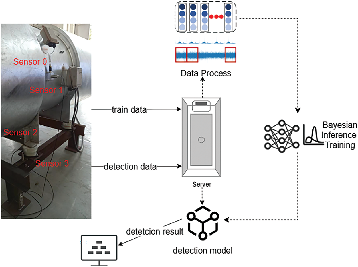
Figure 1: The detection process of bolt loosening based on Bayesian Learning

(1) Data processing: Historical sensor data is systematically collected, including a fan operating state parameter, known bolt loosening labels, and their prior probabilities. The data will be subjected to Fourier transform, then filtered according to the operating frequency. The corresponding amplitudes will be stored. Finally, the data will be reshaped, and the dataset will be divided according to conventional Deep Learning methods.

(2) Model training: In the training process of the Bayesian Learning model, it estimates the probability distribution of each weight parameter. During training, methods such as variational inference and Monte Carlo sampling are employed to perform the calculation of the Evidence Lower Bound (ELBO) loss and the backpropagation process.

(3) Model Evaluation and Interpretability Analysis: The model is evaluated using a test set, assessing both the accuracy and uncertainty of the model on the posterior distribution. Both the uncertainty of the model detection and the importance of the sensors can be analyzed. If the model does not achieve the expected results on the test set, return to Step 2.

(4) Real-time detection: Use the trained Bayesian Learning model to detect and analyze real-time data. It can generate a posterior probability distribution for each potential bolt loosening, which significantly improves the quantitative description and management of detection result uncertainty.

4  Proposed Method

This section first briefly introduces Bayesian Neural Networks, and then elaborates on how to implement multi-sensor bolt loosening detection of the Fan Base based on Bayesian Convolutional Neural Networks.

4.1 Bayesian Neural Networks

The Bayesian Neural Network is the most typical Bayesian Learning model. It considers the weights and biases in the neural network as random variables and estimates the probability distribution of these parameters instead of a single optimal value [32,33], as shown in Fig. 2. In BNNs training, we not only focus on the best fit of the model to the given data, but also on the characterization of prediction uncertainty caused by model parameter uncertainty. In the initialization stage, a prior probability distribution is assigned to each weight and bias, which usually reflects our prior knowledge or assumptions about the reasonable range of parameter values, such as Gaussian distribution, Laplacian distribution, etc. Next, the core stage of Bayesian inference is to calculate the posterior distribution.

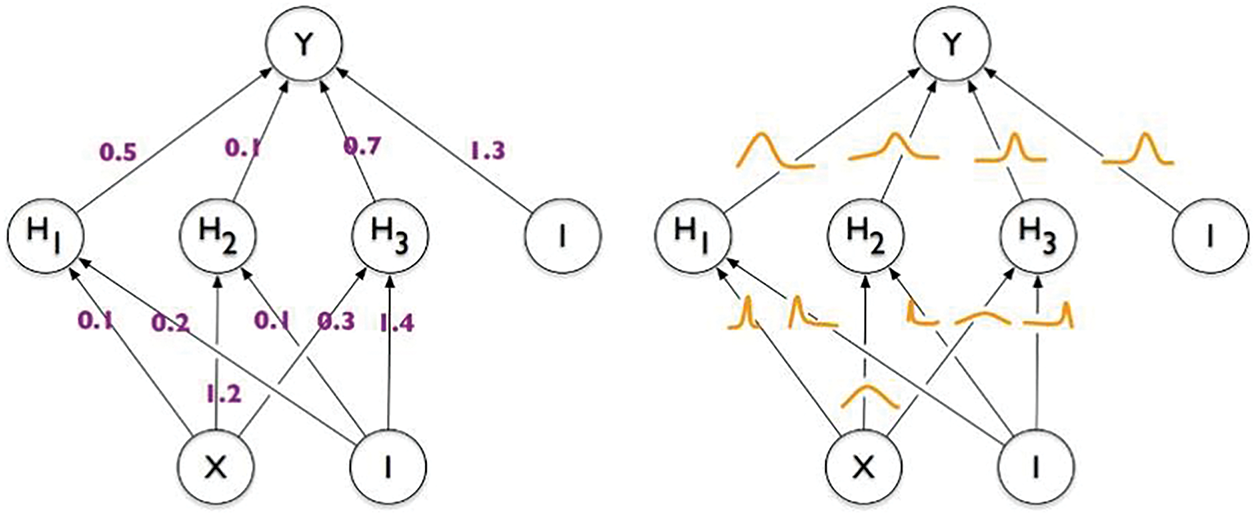
Figure 2: Fixed weights in normal neural networks VS Weight distribution in Bayesian neural networks

Given the observation dataset D, the Bayesian theorem can be used to obtain the conditional probability distribution of parameter W after observing data D. It is the posterior distribution P(W|D), which represents the possible values and probabilities of parameter W under known data conditions. Due to the complexity or even infeasibility of directly calculating the posterior distribution, especially for large neural networks, approximate methods are used. The commonly used approximation method is Markov Chain Monte Carlo (MCMC). It indirectly samples the posterior distribution of sample points by constructing a Markov chain that satisfies specific conditions and simulating the sampling process [34]. Another commonly used method is Variational Inference. It approximates the actual posterior distribution P(W|D) by introducing a parameterized distribution q(w|θ), and then optimizes θ such that q(w|θ) becomes as close as possible to the actual posterior. This process typically utilizes maximizing Evidence Lower Bound (ELBO) and solving gradients through backpropagation algorithms to update variational parameters [35].

Assuming the model parameters are denoted as W, P(W) represents the prior distribution of these parameters. Given observational data D = {X, Y} from industrial equipment, where X consists of input data collected by sensors and Y is the corresponding fault label data, the objective of BNNs is to derive the following distributions:

P(Y|X)=∫P(Y|X,W)P(W|D)dW(1)

wherein:

P(W|D)=P(W)P(D|W)P(D)(2)

P(W|D) represents the posterior distribution, P(D|W) is the likelihood function, and P(D) is the marginal likelihood.

Directly sampling from the posterior probability P(W|D) to evaluate P(Y|X,D) encounters the challenge of high dimensionality in the posterior distribution. To address this issue, variational inference methods are employed. A simpler distribution q(w|θ) is defined to approximate the posterior distribution P(W|D). The variational parameters θ are optimized so that q(w|θ) closely approximates P(W|D) as much as possible. The Kullback-Leibler (KL) divergence is used to measure the distance between these two distributions:

θ=argminθKL[q(w|θ)||P(W|D)](3)

further derivation:

KL[q(w|θ)||P(W|D)]=∫q(w|θ)log⁡(q(w|θ)P(W|D))dw(4)

According to the Bayesian equation, we can derive and organize the expression as follows:

KL[q(w∣θ)||P(W∣D)]=∫q(w∣θ)[log⁡q(w∣θ)[log⁡P(D∣w)−log⁡P(w)+log⁡P(D)]dw(5)

Since log P(D) is a constant term:

KL[q(w|θ)||P(W|D)]=Eq(w|θ)[log⁡q(w|θ)]−Eq(w|θ)[log⁡P(D|w)]−Eq(w|θ)[log⁡P(w)]=−Eq(w|θ)[log⁡P(D|w)]+KL[q(w|θ)||P(w)(6)

Thus, we can observe that by maximizing the expected data likelihood under the variational distribution q(w|θ) while minimizing the KL divergence between q(w|θ) and the prior distribution P(W), we effectively minimize the KL divergence between q(w|θ) and the actual posterior distribution P(W|D) indirectly. Consequently, we define the ELBO as follows:

ELBO=Eq(w|θ)[log⁡P(D|w)]−KL[q(w|θ)||P(w)](7)

4.2 Bolt Loosening Detection Method

This section mainly introduces the configuration of BCNN for bolt loosening detection of the fan base, and also proposes model interpretability, training algorithms, and evaluation algorithms.

4.2.1 BCNN

When conducting fault detection on a fan, multiple sensors are usually fixed on the fan to collect vibration data from various directions and parts. Non-convolutional neural networks are unable to learn the spatial or temporal relationships between multiple sensors and, as a result, cannot effectively integrate data from several sensors. Consequently, they struggle to provide more comprehensive and accurate information about the equipment’s status. This paper combines the Bayesian framework with CNN to detect bolt loosening faults. In the context of multi-sensor data analysis for a fan, BCNN automatically extracts informative features through learning prior distributions and conditional probability distributions. In BCNN, the output of convolutional layers consists of a set of feature maps accompanied by their respective conditional probability distributions, which are derived through linear transformations based on prior distributions. Subsequently, these linear transformations involving both prior and conditional probability distributions can be utilized as inputs to fully connected layers, enabling the extraction of useful features at different scales. Compared to conventional CNN, BCNN excel in handling data with varying scales and distributions and exhibit stronger generalization capabilities. In summary, not only does BCNN inherit BNN’s ability to quantify model uncertainty, but it also excels in hierarchical feature extraction specific to image and signal processing domains. This advancement allows the model to more accurately pinpoint and predict the sources of potential equipment malfunctions.

4.2.2 BCNN for the Bolt Loosening Detection of Fan Base

Configuration of BCNN for the bolt loosening detection of fan base is shown in Fig. 3. It consists of two convolutional layers each including an activation layer, followed by a max-pooling layer after each convolutional layer, and there is a fully connected layer before the final output. The neuron parameters of both the convolutional layers and the fully connected layer follow a Gaussian distribution. The number of input channels in the first convolutional layer is consistent with the number of sensors on the fan. The output of the fully-connected layer corresponds to the number of fault types.

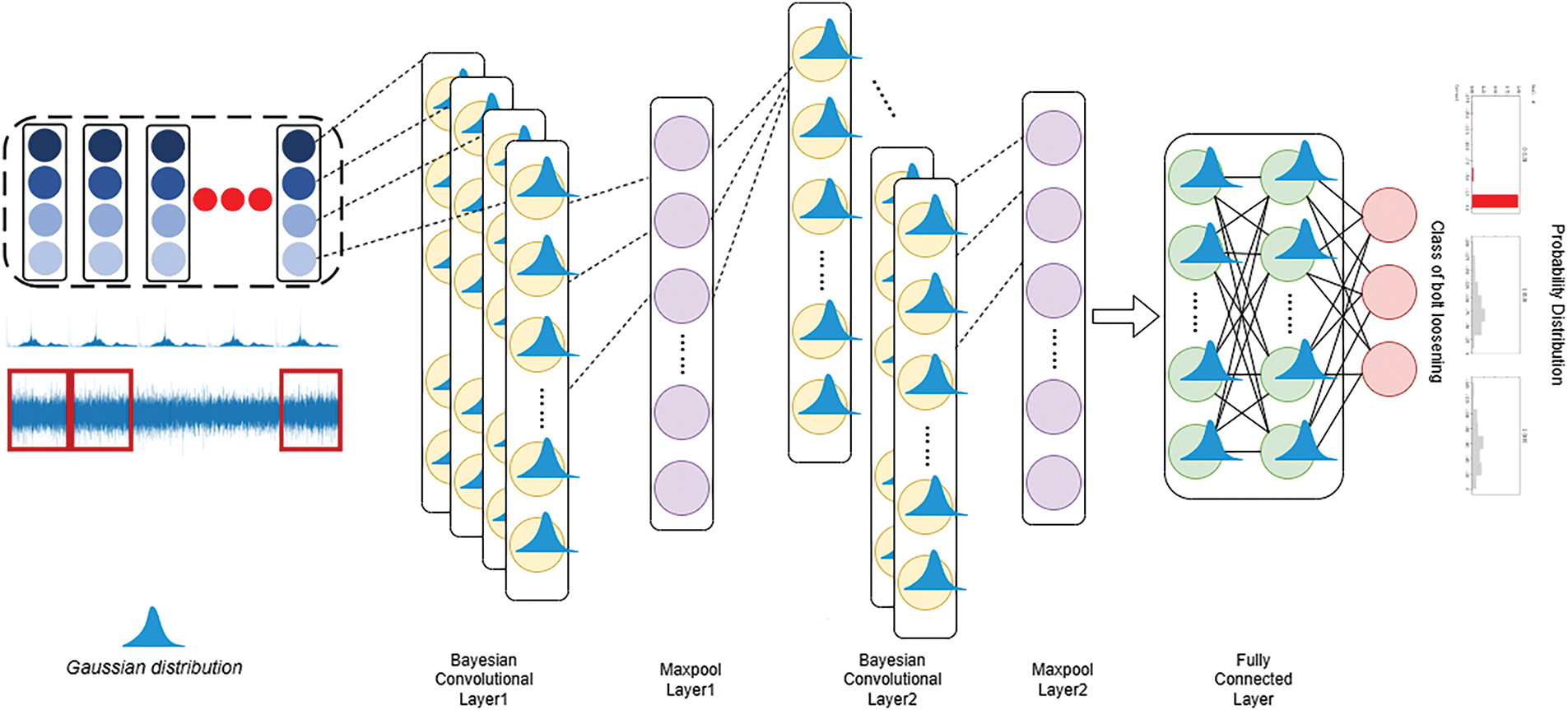
Figure 3: Configuration of BCNN for the bolt loosening detection of fan base

If D represents the input dataset with a shape of (batch_size, c, k), where c denotes the number of channels equivalent to the number of industrial sensors, and k indicates the number of features per channel, when setting up a convolutional layer in the convolutional neural network as (c, i, m), with i being the number of output channels and m representing the size of the one-dimensional convolutional kernel. The mathematical formulation process for BCNN modeling and training based on variational inference is as follows.

Let θ=(μ,σ2), where each weight wi is sampled from a Gaussian distribution N(μi,σi2), with σi being given by the expression σ2=log⁡(1+eρ).

In the practical implementation of BCNN in this paper, the variational posterior distribution is chosen to be a multivariate Gaussian distribution for computation and optimization purposes. For the weights W in a one-dimensional convolutional layer, its variational posterior distribution can be expressed as:

q(W;μ,σ2)=∏c=0n−1∏i=0N−1∏m=0k−1N(W[c,i,m];μ[c,i,m],σ2[c,i,m])(8)

here, μ and σ respectively denote the mean and variance parameters for the weights W, which are also variables to be optimized. Similarly, in order to ensure regularization effects and numerical stability, the variance can be constrained to be non-negative using a “softplus” function or other transformations:

σ2[c,i,m]=softplus(ρ[c,i,m])(9)

ρ represents another learnable parameter.

For such a variational posterior distribution, the data likelihood term in the computation of the ELBO can also be obtained through gradients using the reparameterization trick:

W∼q(W;μ,σ2)⇒W=μ+ε⊙σ(10)

ε∼N(0,I)(11)

Thus, the data likelihood term can be approximately expressed as:

Eq(w;μ,σ2)[log⁡p(Y|X,W)]≈1L∑l=1Llog⁡p(Y|X,μ+εl⊙σ)(12)

L is the number of samples and εl is an independently and identically distributed (i.i.d.) noise drawn from a standard normal distribution.

For the KL divergence term, in the case of a multivariate Gaussian distribution in one dimension, its analytical computation remains unchanged.

KL[q(W;μ,σ2)||p(W)]=12∑c,i,m(log⁡σp2σ2[c,i,m]+σ2[c,i,m]σp2+(μ[c,i,m]−μp)2σp2−1)(13)

μp and σp2 respectively denote the mean and variance of the prior distribution for the weights W in the one-dimensional convolutional layer.

Ultimately, the optimization objective remains to maximize the ELBO, which is achieved by updating the μ, ρ, and σ parameters through gradient descent or other optimization algorithms. This process aims at minimizing the KL divergence while maximizing the data likelihood.

In the context of BCNNs (including scenarios involving one-dimensional convolutional kernels), we now have the components necessary for computing the ELBO:

ELBO(q)=Eq(w;μ,σ2)[log⁡p(Y|X,W)]−KL[q(W;μ,σ2)||p(W)](14)

The data likelihood term is given by Eq. (12), and the KL divergence is represented by Eq. (13).

The maximization of ELBO is accomplished through gradient ascent. We compute the gradients of ELBO with respect to the variational parameters μ and ρ (or indirectly σ). For this purpose, we need to calculate the gradients for both the data likelihood term and the KL divergence term separately.

The gradient of the data likelihood term can be computed using the chain rule and backpropagation:

∇μ,ρEq(W;μ,σ2)[log⁡p(Y|X,W)]≈1L∑l=1L∇μ,ρlog⁡p(Y|X,μ+εl⊙σ)(15)

The gradient of the KL divergence term can be computed directly since it is an explicit function of the variational parameters with derivatives taken separately for μ and ρ:

∇μKL[q(W;μ,σ2)||p(W)]=−1σp2(μ−μp)(16)

∇ρKL[q(W;μ,σ2)||p(W)]=1σp2(eρ1+eρ−μ2+σp2σ2)(17)

In this case, we know that σ2=softplus(ρ), and when taking the derivative with respect to ρ, we use the derivative of the softplus function, which is 11+e−ρ.

Note that the BCNN for bolt loosening detection in this paper performs gradient computations under the assumption that the prior distribution P(W) is also a multivariate Gaussian distribution, with known mean μp and variance σp2.

For the gradient expressions of μ and ρ, they can be derived by taking the derivative of each term within the original KL divergence expression.

Subsequently, we sum up these gradients and take the negative of this sum to obtain the negative gradient. Using this negative gradient, we then update the variational parameters:

μ←μ−η∇μELBO(18)

ρ←ρ−η∇ρELBO(19)

where η represents the learning rate. By iteratively following this update process, we gradually approach the optimal variational parameters that maximize the ELBO. Throughout this process, the model continually refines the distribution of weights to better fit the training data while maintaining a degree of uncertainty to prevent overfitting.

Based on variational inference, BCNN provides an effective predictive approach in bolt loosening detection. They not only deliver probabilistic predictions of bolt loosening but also quantify the uncertainty within the model, which holds significant value for preventive maintenance and decision support. Furthermore, by optimizing the ELBO loss function, we can obtain a model that exhibits both strong predictive performance and robust generalization capabilities.

The BCNN model training algorithm (Algorithm 1) for bolt loosening detection is as follows. In the algorithm, the SVI function involves the variational inference objective function ELBO, as well as the backpropagation updates to parameter θ based on the Eqs. (14)–(19).

4.2.3 Interpretability

(1) Uncertainty estimation of the detection results

In the detection of bolt loosening fault, accurately assessing and predicting uncertainty is crucial for preventive maintenance and decision-making support. BCNN can quantify the uncertainty of model predictions by introducing the prior and posterior distributions of parameters. Let the input data X be the fan operation data collected by sensors, and the posterior distribution of model parameters be P (W│D). By sampling multiple sets of weight vectors {Ws}s=1S from this posterior distribution, the corresponding bolt loosening probabilities P(Y|X,Ws) can be calculated. Here, Y represents whether the fan has bolt loosening or the classification of bolt loosening fault.

By calculating the mean and variance of these predicted probabilities, we can obtain the expected value of the prediction results and the associated uncertainty. The equation for calculating the expected value is as follows:

E[Y|X]=1S∑s=1SP(Y|X,Ws)(20)

This value is obtained by calculating the loosening probabilities using multiple sets of weights sampled from the posterior distribution and then taking the average. It represents the expected probability of bolt loosening when parameter uncertainty is considered. A larger value indicates that the model as a whole tends to determine that there is a risk of bolt loosening. In addition, by analyzing the probability distribution of the results from all sampled models, after setting a threshold, we can output a measure of uncertainty for unseen data, rather than simply making a direct determination based on the training labels.

The equation for calculating the variance is as follows:

D[Y|X]==1S∑s=1S(P(Y|X,Ws)−E[Y|X])2(21)

The larger the variance, the more significant the differences in prediction results under different parameter samplings, indicating higher uncertainty and a correspondingly wider confidence interval. A relatively large variance suggests that the model’s judgment on the current bolt status is less reliable, requiring priority for manual review. Conversely, a small variance indicates that the prediction results are more credible and can be directly used as a basis for maintenance decisions.

(2) The influence degree of each sensor and its related characteristics

Under the BCNN model described in Section 4.2.3, where c represents the number of sensors (or the number of input channels), i represents the number of output channels of a given layer, and m is the size of the convolution kernel. The dimension of the weight matrix of the one-dimensional convolutional layer in the model is (i, c, m). The weight wi,c,j (where j indexes the position within the convolution kernel) represents the contribution weight corresponding to the feature extracted from the j-th position of the input channel c (corresponding to a sensor in a certain direction) when calculating a certain feature in the current output channel i. Its magnitude directly reflects the degree of influence of this sensor feature on the output.

After the model training is completed, the posterior distribution P(wi,c,j|D) (which is usually in the form of a Gaussian distribution, but it could also be a more complex distribution) of the weight wi,c,j is obtained. It can be described by mean and variance matrices.

The mean of weights reflects the average importance of features. The calculation equation is as follows:

μi,c,j=E[wi,c,j|D]=∫wi,c,jP(wi,c,j|D)dwi,c,j(22)

The expected value of the weight reflects the importance of the corresponding sensor and its local features. If the expected value is relatively high and positive, it indicates that this sensor has a significant impact on the probability of bolt loosening.

The variance of weights reflects the uncertainty in the importance of features. The equation for calculating the weight variance is as follows:

σi,c,j2=E[(wi,c,j−E[wi,c,j|D])2|D](23)

The larger the variance, the higher the uncertainty in assessing the importance of the feature, indicating that the model has not yet stably learned the correlation between this feature and bolt loosening. The standard deviation σi,c,j, as the non-negative square root of the variance, also conveys this uncertainty and has the same unit as the weights, providing a more intuitive understanding.

If the weights are i.i.d., the variance matrix is likely to be a diagonal matrix, and its diagonal elements represent the variance σi,c,j2 of each weight. However, when there are correlations among the weights, a non-diagonal covariance matrix is used. The non-zero off-diagonal elements in it represent the degree of correlation between different weights. The shape of this covariance matrix is the same as that of the weight matrix, covering the relationships among all possible weight combinations in the model. For example, features from sensors in different directions may jointly affect the loosening detection results.

4.2.4 Model Evaluation

This paper evaluates the model by combining the uncertainty estimation of interpretability mentioned above. This paper mainly evaluates two aspects: accuracy of the test set and estimation of uncertainty. The impact of various sensors and their related features is also analyzed.

(1) The accuracy of the model

The paper presents a method to assess prediction uncertainty for the fan sensor data. For a BCNN model that has been trained, the process begins with defining a sampling number nsampling. The purpose is to effectively sample the model’s parameter space using its posterior distribution, thereby generating nsampling independent model instances. For each data in the test set, these nsampling models are used to produce and record their respective predictions. By calculating the mean vector of these multiple model outputs, we can infer the most likely state or classification for each sample. This is achieved by identifying the index corresponding to the maximum value in the ensemble average prediction vector.

In addition to the overall accuracy on the test set, to delve deeper into the model’s performance in classifying number of loose bolts, we separately calculate the accuracy. We compare the actual labels with the predicted classification of the model to gain a comprehensive understanding of the model’s performance differences in identifying bolt loosening when analyzing fan sensor data.

The accuracy evaluation algorithm of the BCNN model for bolt loosening detection (Algorithm 2) is as follows:

(2) the estimation of uncertainty

The paper proposes a method for evaluating the uncertainty of bolt loosening fault. Firstly, for each of the above nsampling models, corresponding prediction results are output, and the class probability distribution is calculated for the given input sensor data. To enhance numerical stability, prevent overflow issues, and facilitate subsequent processing, the class probability distributions are represented in log-probability form. The resulting set of log-probability distributions is of shape (nsampling, N, C), where N denotes the number of samples and C represents the number of classes.

Subsequently, for each class, the median of the probability distribution is adopted as a representative or benchmark probability value to provide a robust and outlier-resistant probability estimate. Alongside this, the model sets a threshold where if the median probability given by the model for a particular class exceeds this threshold, it is considered highly likely that the class corresponds to the actual prediction result. When the median probability of a class surpasses the set threshold, it is flagged as a potential predicted class and its count is accumulated. Concurrently, all median probabilities meeting the threshold condition are saved. The index corresponding to the maximum saved median probability is used as the model’s predicted class for the current situation. However, should all median probabilities fail to reach the pre-set threshold, it strongly suggests that there is a high degree of uncertainty in the input industrial data with respect to the current known classification system, which could indicate the emergence of an unknown new fault class. In such a scenario, the model determines the prediction result as “undecided,” signaling the need for further in-depth data mining, model optimization updates, or exploration into whether new fault class exists.

The uncertainty evaluation algorithm of the BCNN model for bolt loosening detection (Algorithm 3) is as follows:

5  Experiment and Results

This section introduces experimental preparation for the real-world fan base, and presents and analyzes the experimental results.

5.1 Experiment Preparation

This section introduces the experimental scenario of factory fans, the generated dataset, the setting of experimental parameters, and the data processing methods.

5.1.1 Experimental Scenarios and Datasets

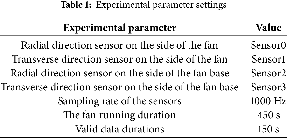
This paper presents data collected from a flow fan manufacturing factory in Zhejiang Province, China. The object of the data collection is a specific model of axial flow fan manufactured by the factory, equipped with four vibration sensors to capture vibrational data in four distinct directions. As shown in Fig. 1, the positions of Sensor0 and Sensor1 are radial and transverse directions on the side of the fan, while Sensor2 and Sensor3 are positioned at the radial and transverse directions on the fan base. The sampling rate of the sensors is set at 1000 Hz. During experimentation, both normal operational conditions and four distinct fault scenarios are simulated for the fan: impact, rotor imbalance, looseness of one base bolt, and looseness of three base bolt. Under each condition, data are collected from the fan’s startup until shutdown, spanning approximately 450 s. However, following time-domain analysis, the valid experimental data are limited to roughly 150 s of stable operating data after the fan reaches its equilibrium state, which further underscores the inherently small dataset characteristic of this scenario. The specific settings of the aforementioned experimental parameters are shown in Table 1.

5.1.2 Spectrum Method for Bolt Loosening Detection

In vibration signal analysis, time-frequency analysis is one of the most used methods for fault detection. It simultaneously reveals changes in a signal’s characteristics over time and frequency domains, making it particularly effective for non-stationary or transient vibration signals, whose features typically vary with time. The Fast Fourier Transform (FFT) is a classical method, but it assumes the signal is stationary and decomposes the signal into sinusoidal components of different frequencies. It is not suitable for analyzing vibration signals under varying operating conditions of rotor systems. The equation for the Fourier Transform is expressed as follows:

F(ω)=∫−∞∞f(t)e−iωtdt(24)

The Fourier Transform converts a time-domain signal f(t) into a frequency-domain signal F(ω). This transformation enables us to better understand the characteristics of the signal, such as its frequency components and periodicity, among others. Through Fourier spectrum analysis, the industrial fan data mentioned above can be analyzed to identify the axial frequency of the fan at 24.8 Hz, and faults like impacts and rotor unbalance can be distinctly recognized.

In this paper, the normal spectrum of the industrial fan, the spectrum for a case with one loose bolt, and the spectrum for a case with three loose bolts are respectively presented in Fig. 4 (Due to the position and direction of sensor2, taking sensor2 as an example). From these figures, it can be observed that the spectral characteristics typical of such faults are not clear. A direct comparison of these spectra reveals a critical flaw in traditional spectral analysis for bolt loosening detection: it lacks clear and stable fault-specific features, making it unable to reliably distinguish between normal and loosened states, let alone quantify the degree of loosening. In Fig. 4, the spectra of one loose bolt and three loose bolts show almost no obvious differences, despite the varying degrees of loosening. This is because loosening causes complex interactions (such as uneven load distribution and structural deformation), which disrupt the linear relationship between the degree of loosening and spectral features. Unlike the simple logic of “the more severe the loosening, the more significant the spectral changes”, these signals do not follow a predictable pattern, resulting in traditional methods being unable to determine the degree of loosening or even confirm whether loosening has occurred. In summary, traditional spectral analysis methods have fundamental flaws: they cannot extract weak signals from noise, cannot handle nonlinear relationships, and cannot resolve the issue of feature overlap.

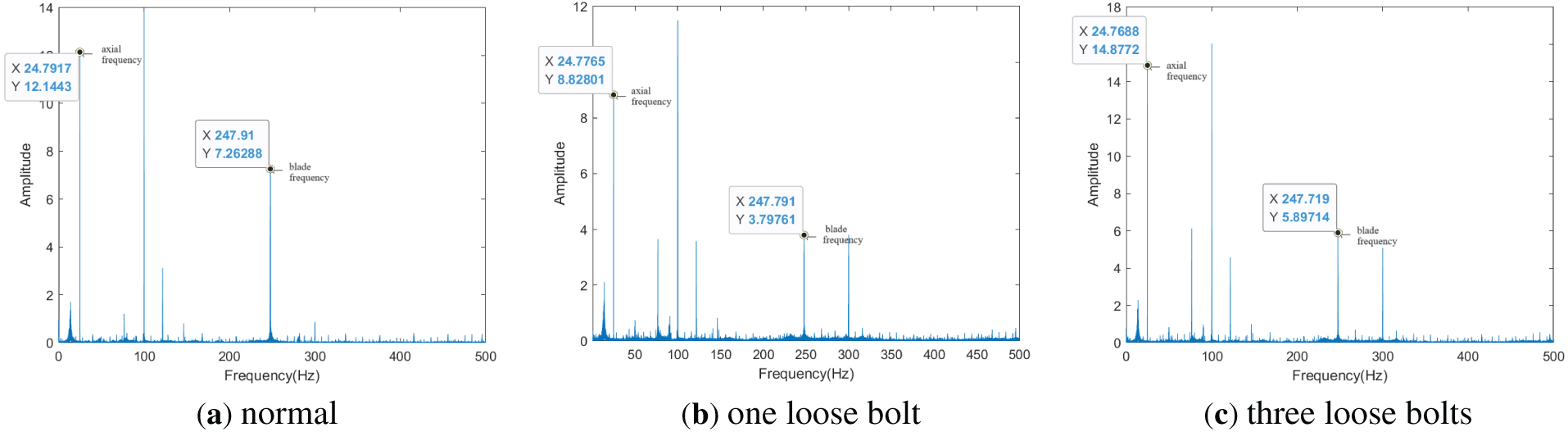
Figure 4: Spectrum of Sensor 2 in three different scenarios

5.1.3 Experimental Environment and Parameter Definition

This paper utilizes a Dell PowerEdge R740 server with advanced hardware configurations as the experimental platform. The server is powered by a dual Intel Xeon Gold 5218R processor setup and possesses 256 GB of memory. Although the server is also provisioned with two NVIDIA Tesla T4 GPUs to manage large-scale parallel computing and Deep Learning tasks, due to the relatively smaller scale of data involved in the experiments presented herein and the adequacy of the CPU performance to satisfy the requirements of the current experimental setting, the GPUs are not utilized during the actual execution of the code. The server operates on the Ubuntu 22.04 LTS operating system and runs version 1.3.0 of the PyTorch Deep Learning framework, which is utilized to construct and execute the experiments.

In the implementation of BCNN, this paper utilizes Pyro, a contemporary probabilistic programming library. Pyro is a flexible framework built atop Python and PyTorch specifically designed for the development of Bayesian Deep Learning models and other intricate probabilistic models, first released in 2017 by Uber AI Labs. Constructed upon the foundation of the PyTorch Deep Learning framework, Pyro harnesses PyTorch’s dynamic computation graphs and automatic differentiation capabilities, offering users a highly adaptable and powerful platform to design, simulate, and infer complex probabilistic models [36]. Pyro comes equipped with a rich set of tools to define random variables, construct implicit or explicit probabilistic models, and perform efficient and modular inference through methods such as variational inference and Markov Chain Monte Carlo algorithms. This integration allows researchers and developers to seamlessly blend Deep Learning architectures with Bayesian principles, enabling them to tackle problems with uncertainty quantification and probabilistic reasoning effectively.

In the experiment, the CNN model consists of two 1D convolutional layers, each with 16 and 32 output channels, respectively, and a kernel size of 3. Following each convolutional layer, there is a ReLU activation function and a max pooling layer to extract and reduce the dimensionality of the features. After passing through these two consecutive sequences of convolution-activation-pooling operations, the flattened features are then mapped onto three classes via a fully connected layer, making the model suitable for small-scale multi-classification tasks. The loss function used for the comparative conventional CNN model is cross-entropy. Across all models, the learning rate is set to 0.01, the number of training epochs is 500, and the batch size is 8. When performing model evaluation for the BNN model, the parameters are sampled 100 times to account for uncertainty estimation and to provide a probabilistic interpretation of the model’s predictions. This paper compares the performance of BCNN with conventional CNN, BNN and Transformer.

5.1.4 Data Processing

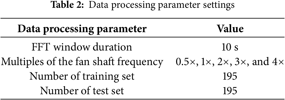
For each of the three scenarios (normal, one loose bolt, and three loose bolts), effective segments of data are subjected to FFT, with an FFT window duration of 10 s. An FFT is performed once per second, resulting in 130 sets of data per scenario (take 131 s from 150 s data). After the FFT, the 0.5×, 1×, 2×, 3×, and 4× multiples of the fan shaft frequency are extracted. Consequently, for each set of data, there are four sensors, each providing five frequency data points, thus creating a dataset with a shape of (4, 5) per set. In total, there are 390 sets of data. To highlight the advantages of BCNN in handling small dataset, the data is split into a training set and a test set in a 5:5 ratio, ensuring balanced quantities of data for each class. This means that for each of the three classes, equal amounts of data are allocated to both the training and test subsets. The specific settings of the aforementioned data processing parameters are shown in Table 2.

5.2 Experimental Results

This section presents experimental results, including model training effectiveness, accuracy, confidence intervals, uncertainty estimation, and interpretability analysis.

5.2.1 Model Training Effectiveness

The loss of CNN model training is shown in Fig. 5a, the loss of BNN model training is shown in Fig. 5b, the loss of BCNN model training is shown in Fig. 5c, and the loss of Transformer model training is shown in Fig. 5d. The CNN and Transformer model exhibits significant fast convergence during training, with its cross-entropy loss function value rapidly decreasing to a lower level. This reveals that the model has efficient learning ability and parameter optimization efficiency, but overfitting may occur. BNN and BCNN, on the other hand, use the ELBO loss function for training. Compared to CNN and Transformer, their convergence speed appears to be slower, and the loss value fluctuates during the training process. The convergence of BCNN is slower than BNN, and there are more obvious oscillations. BCNN may face certain complexity and uncertainty in the process of finding the optimal solution.

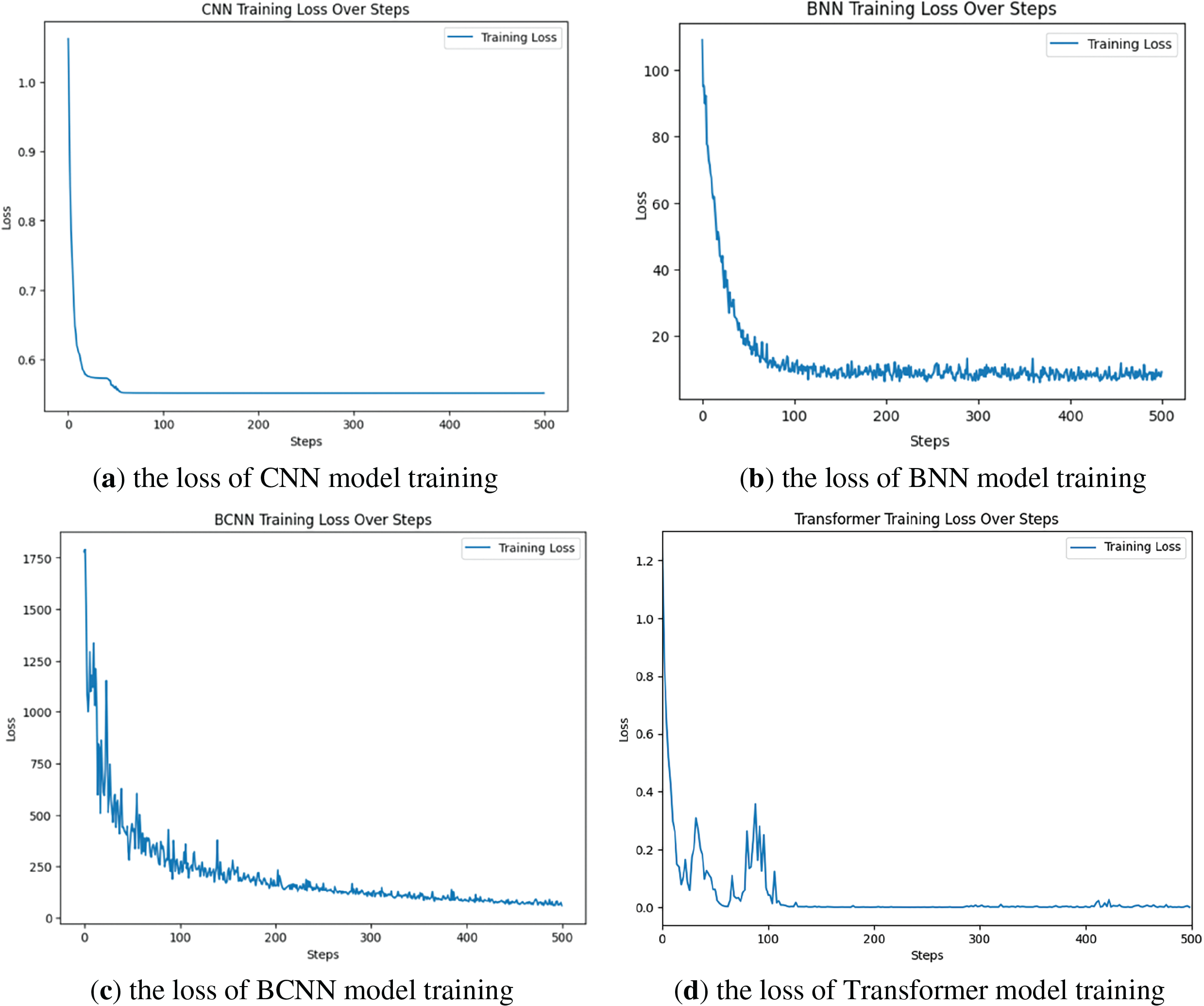
Figure 5: Comparison of training losses for three models

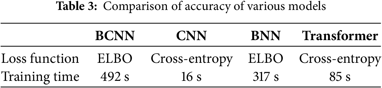
As shown in Table 3, BCNN has the longest training time. Although BCNN incurs higher computational cost when calculating losses due to its incorporation of the Bayesian probability framework to estimate the probability distributions of model parameters rather than single definitive values, this design choice is intended to bolster the model’s generalization performance and capacity for uncertainty modeling. After undergoing a greater number of iterative training steps, the ELBO loss of the BCNN eventually converges successfully, indicating that despite initial differences in performance, the BCNN model is still able to attain a stable learning state across various potential scenarios, demonstrating strong adaptability to new data and accurate predictive abilities.

5.2.2 Accuracy

According to the accuracy evaluation method described in Section 4, combined with the performance of the model on the test set, the accuracy results are shown in Table 4.

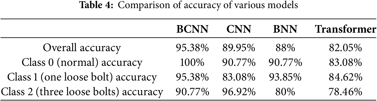
In terms of overall accuracy, BCNN still maintains the highest level, reaching 95.38%, which is better than CNN’s 89.95%, BNN’s 88% and Transformer’s 82.05%. This indicates that BCNN has the best overall classification performance.

For normal (Class 0), BCNN maintains a perfect accuracy of 100%, showing stronger discriminative ability compared to CNN’s 90.77%, BNN’s 90.77% and Transformer’s 83.08%.

For one loose bolt (Class 1), the accuracy of BCNN is 95.38%, significantly higher than CNN’s 83.08%, Transformer’s 84.62% and slightly higher than BNN’s 93.85%, indicating that BCNN has higher accuracy in handling bolt loose.

For three loose bolts (Class 2), the accuracy of BCNN is 90.77%, lower than CNN’s high accuracy of 96.92% in this class, but significantly better than BNN’s 80% and Transformer’s 78.46%. Although BCNN does not perform as well as CNN in this specific class, it still has an advantage in overall balance and stability.

BCNN exhibits high stability and accuracy in various classes.

The amplitude data of harmonic frequencies in vibration signals are essentially sparse local features in the frequency domain. The convolution kernels of CNN can directly capture these local frequency patterns through parameter sharing. Although the self-attention mechanism of Transformer can model global dependencies, it is difficult to learn effective correlations from sparse harmonic frequency amplitudes with small datasets. When the number of samples in the dataset is very small, the attention weights of Transformer may fail to distinguish the differences in frequency distribution between “normal” and “loosened” states, leading to classification confusion. The harmonic frequency amplitudes after Fourier transform are discrete frequency points, lacking temporal or spatial continuity. The positional encoding design of Transformer is more suitable for sequence data with an inherent order, whereas the “positions” (frequency points) of harmonic frequency amplitudes do not have a natural physical sequential meaning. In contrast, CNN can directly process local patterns in the frequency dimension through 1D convolution. If Bayesian methods are combined with Transformer, Bayesian Transformer has a large parameter scale. With small datasets, variational inference or MCMC sampling struggle to accurately estimate the posterior distribution. Small datasets cannot provide sufficient information to constrain the uncertainty of a large number of parameters. Therefore, the performance may be even worse.

5.2.3 Confidence Interval

In order to clearly and intuitively reveal the trend distribution characteristics of uncertainty associated with different classification results in the entire test set, this paper first classifies the test samples in an orderly manner according to class 0, 1, and 2, and uses them as the horizontal axis to construct a curve graph. Fig. 6 corresponds to the posterior distribution classification results for class 0, 1, and 2, respectively. The vertical axis is used to represent the log-probability distribution of each class predicted by the model. The blue curve depicts the trend of the mean posterior probability of the samples, while the shaded area shows the 95% confidence interval range corresponding to each sample, revealing the differences in uncertainty of the model for different classification judgments.

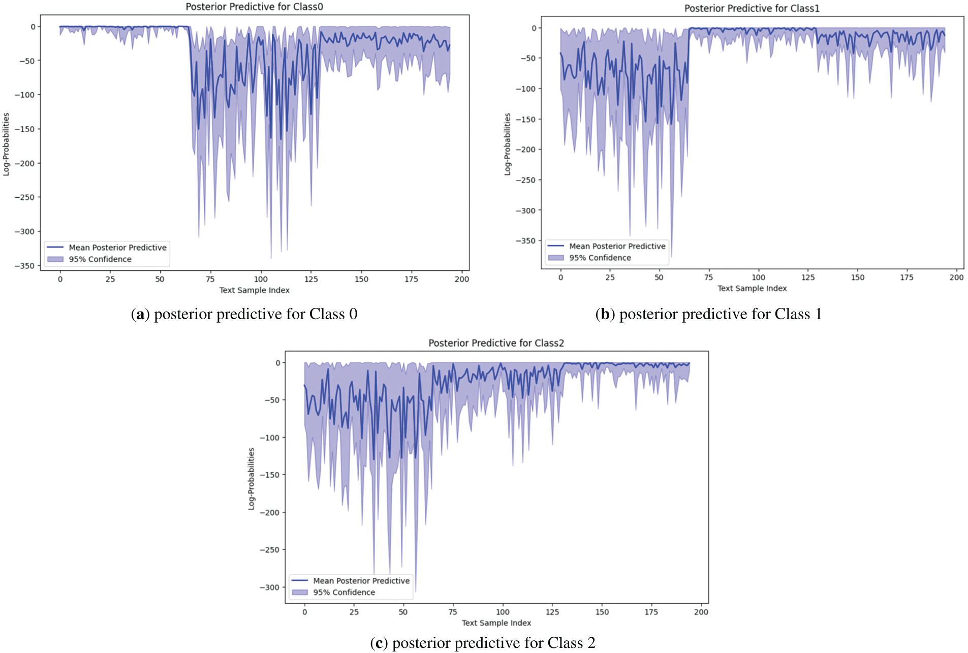
Figure 6: Posterior distribution prediction classification results

From the figures, it is clear that for each class, the model generates mean log-probabilities that reach their highest levels for the correct class, and these log-probabilities are accompanied by relatively narrow confidence intervals. This phenomenon strongly suggests that the model shows a high level of accuracy and strong certainty when predicting various classes.

Specifically, in the classification prediction figure for Class 0, the probability mean curve conspicuously exceeds those of other classes, and the corresponding confidence interval is visibly narrower. This revelation underscores that the model not only accurately detects Class 0, but also holds a high degree of confidence in its predictions for this condition. Conversely, in the classification prediction figures for other classes, wider confidence intervals indicate more uncertainty in the model’s determination of other faults. Upon closer inspection of the probability distributions for Class 1 and 2, while their respective mean curves exhibit some degree of distinction, they are not vastly different from each other compared to Class 0. Additionally, the shaded parts representing their confidence intervals show relatively proximate ranges. This signifies that when distinguishing the number of loose bolts in the fan is one or three, the model encounters challenges and is more prone to misclassification errors.

In summary of the above analysis, the model has a clear discriminative effect on the normal operation status of the fan and loose base bolts. Although different fault levels caused by different numbers of loose bolts can be roughly detected, the boundary between these two fault levels is relatively fuzzy and uncertain in actual classification. This conclusion is consistent with actual fan maintenance experience, that is, there is a significant difference between the stable operation status and the vibration characteristics caused by s loose base bolt, while the vibration characteristics reflected by the same type of loosening fault (with different numbers of bolts) are relatively weak and difficult to detect.

5.2.4 Uncertainty Estimation Results Based on Unknown Data

According to the analysis and evaluation process described in Section 4, select one representative data from each of the three classes in the test set and input it into the model. The classification results are shown in Fig. 7. The model outputs three sub-figures for each sample, representing the histograms of the three classes of results. The horizontal axis of the sub-figure represents the log-probability of the sample in each sampling model, divided into 8 equal intervals. The vertical axis represents the frequency density of the probability of falling into each interval. If the median probability exceeds the set threshold of 0.3, the corresponding histogram icon of the sub-figure is red, and the predicted value is output as “Real:”.

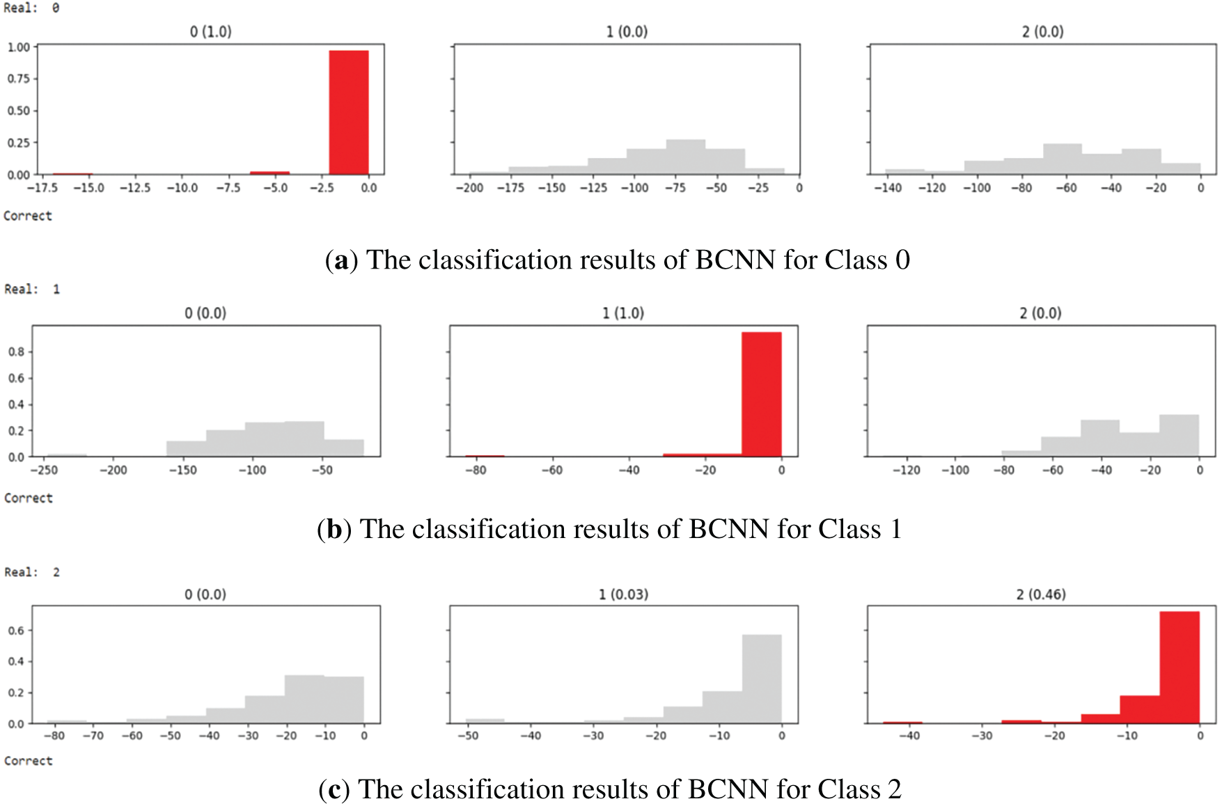
Figure 7: Classification results of BCNN

The results show that all representative three data in the test set can accurately predict the detection results.

In order to verify the uncertainty evaluation performance of BCNN in handling unknown faults and compare the effectiveness of non-Bayesian models, this paper generated 100 sets of uniformly shaped random numbers as unknown fault data. These datasets are input into BCNNs and conventional CNNs for comparative analysis.

Using three representative data as examples, the results are presented. The output result of the CNN model is a probability value vector for three classifications, and the maximum probability should be taken to represent the corresponding classification. The result is as follows.

[3.1826412e−04 9.8696369e−01 1.2718096e−02]

[1.8584278e−05 9.9604779e−01 3.9335098e−03]

[2.1771020e−04 9.4495398e−01 5.4828204e−02]

The results indicate that all three sets of unknown data are classified as Class 1 faults.

The same three sets of data are input into BCNN, and the results are shown in Fig. 8. The absence of red highlights in the sub-figure indicates that the classification probability threshold has not been reached. The output conclusion of the model is undecided, indicating that it is detected as an unknown and uncertain fault type.

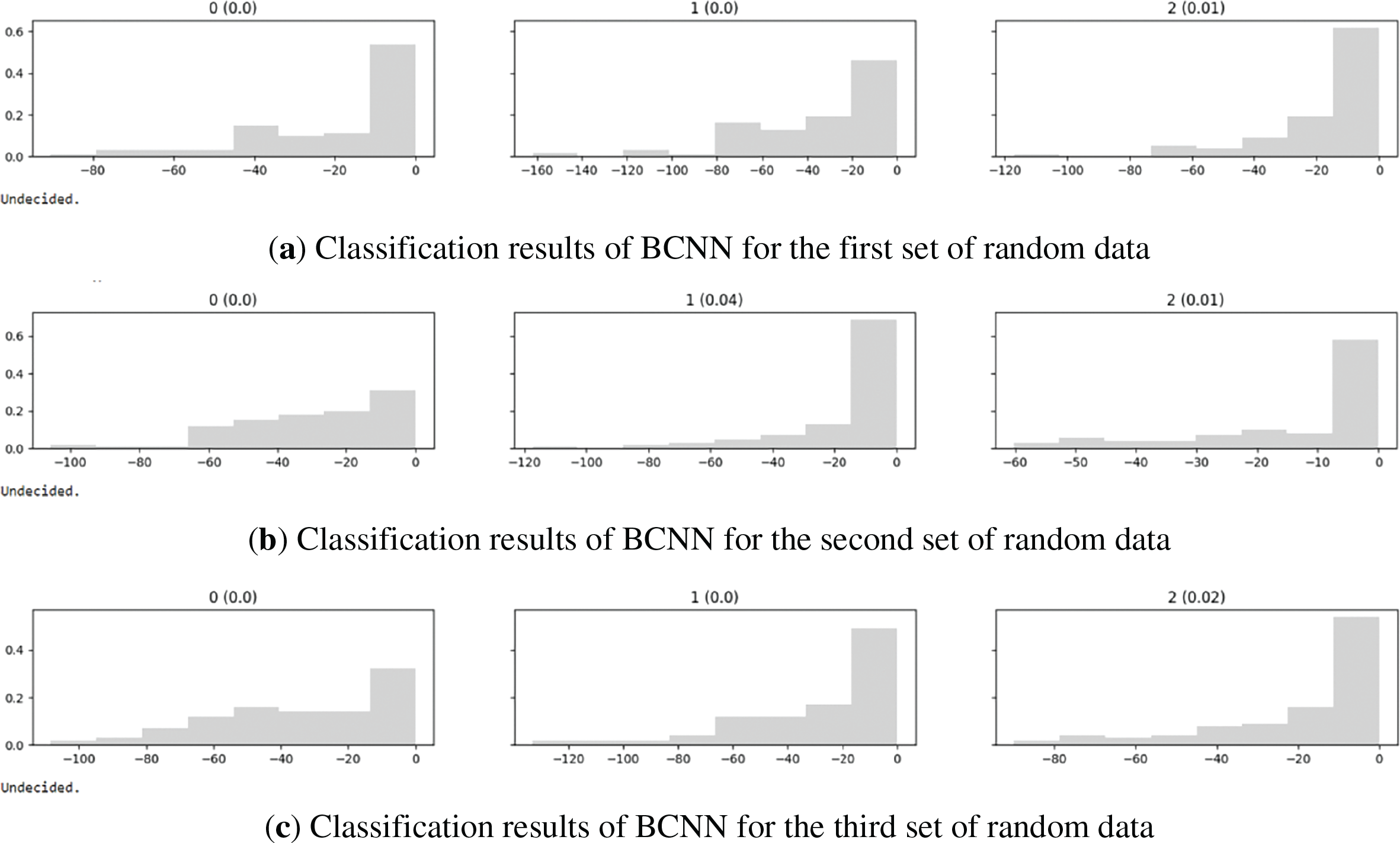
Figure 8: Classification results of BCNN for random data

The experimental results revealed that the actual fault data in the test set exhibited a highly deterministic probability distribution feature for a specific class of results in the model prediction stage, indicating that the model has clear and stable judgment ability for data with known faults. On the other hand, for unknown random data, the output of the BCNN model exhibits significant uncertainty characteristics and can provide uncertain judgment results, which precisely reflects the model’s ability to accurately quantify the degree of uncertainty in its decision-making in unknown fault situations. In contrast, conventional CNN directly provides a classification conclusion in probabilistic form when dealing with such unknown data, resulting in incorrect classification results and inability to identify unknown class. Therefore, the experimental results strongly demonstrate that BCNN not only has accuracy in classifying known fault, but also exhibits excellent uncertainty modeling performance in handling unknown fault scenarios.

5.2.5 Interpretability Results of Features

According to the statement in Section 4.2.3, in the analysis of the results obtained after training BCNN, this paper presents the visualization results of the parameters. By drawing the expected heatmaps and standard deviation heatmaps of the weights for each layer of the model, we can reveal its inherent characteristics. For 1D convolutional layers in this experiment, weight parameters have three dimensions (number of output channel, number of input channel number, convolution kernel size). In the generated heatmap, the input channel number and convolution kernel size are flattened as the horizontal axis to visually display the distribution of expected weight values under the interaction of each output channel with all input channels and convolution kernels. The vertical axis represents the number of output channels. For the fully connected layer, the heatmap is constructed with the input feature dimension as the horizontal axis and the output class of the classification task as the vertical axis. The color depth of the heatmap corresponds to the final calculated numerical value, which helps us to deeply analyze the impact and uncertainty of each weight parameter on the output results of the corresponding layer. Furthermore, through this visualization method, we can indirectly evaluate the significance and uncertainty of the impact of sensors and their generated data sequences on the overall classification results. Fig. 9 shows the expected heatmap and standard deviation heatmap of the first convolutional layer weight. Fig. 10 shows the expected heatmap and standard deviation heatmap of the second convolutional layer weight. Fig. 11 shows the expected heatmap and standard deviation heatmap for output fully connected layer weight.

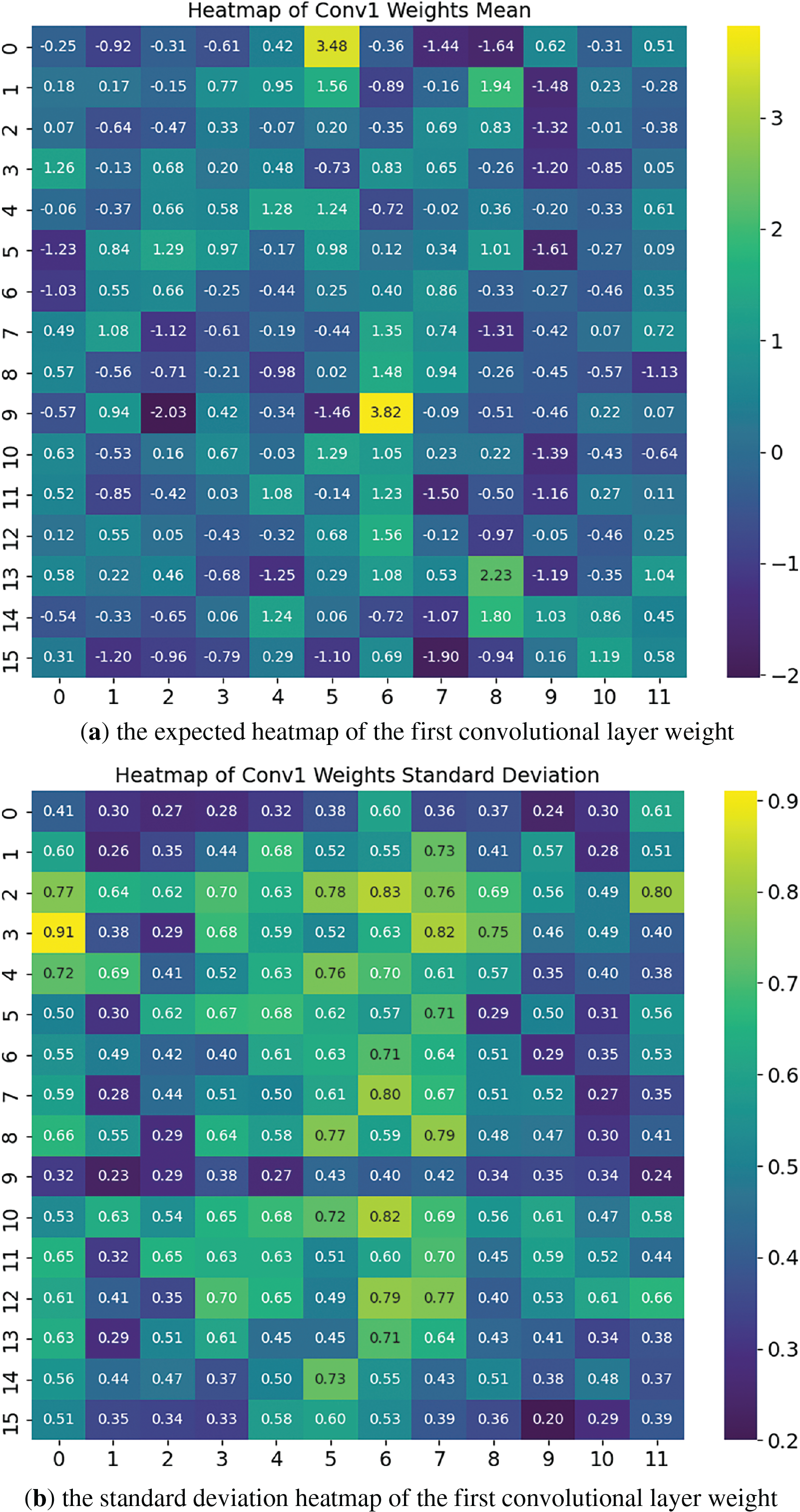
Figure 9: Heatmap of the first convolutional layer weight

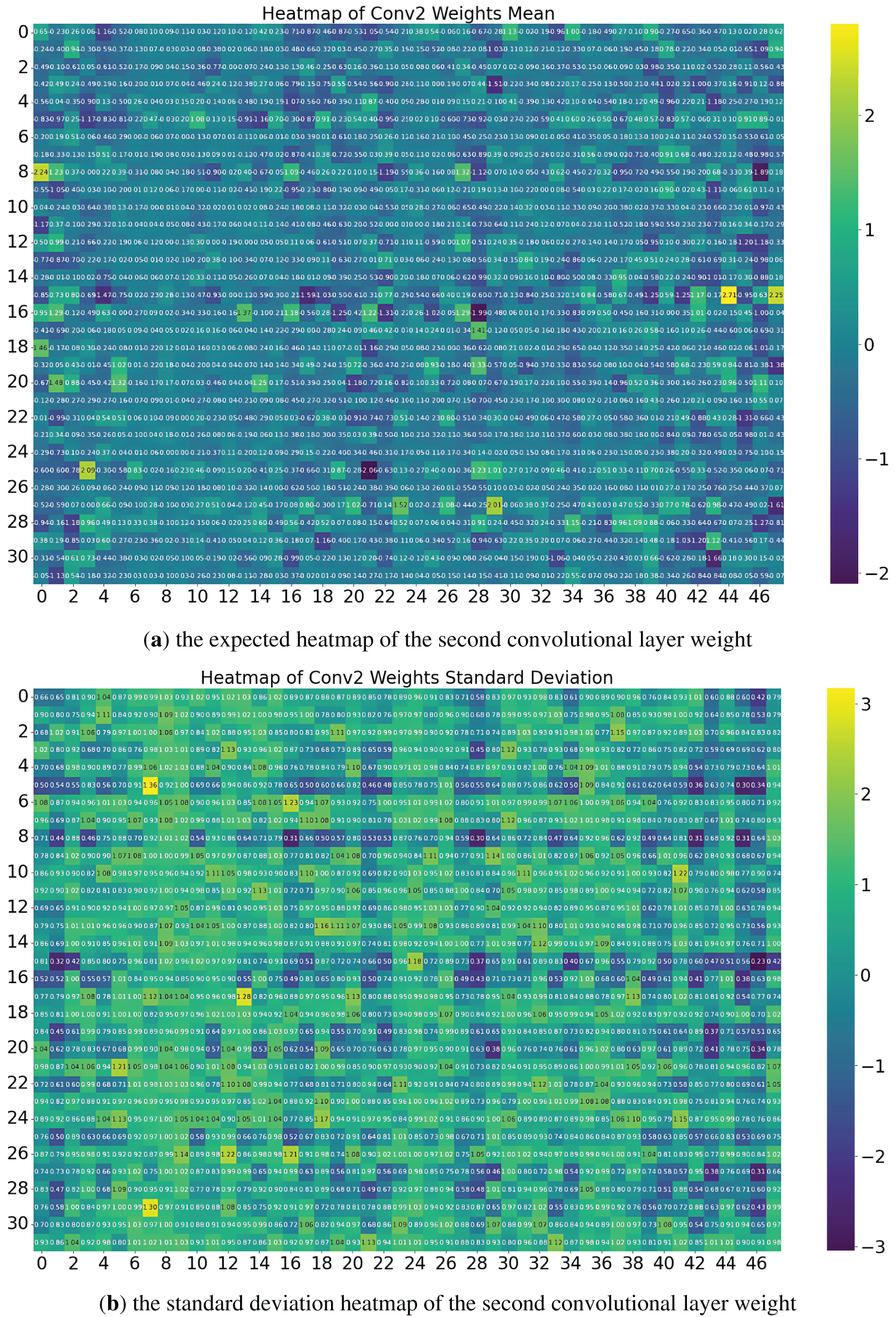
Figure 10: Heatmap of the second convolutional layer weight

Figure 11: Heatmap of the output fully connected layer weight

According to the algorithm in Section 4.2.3, From a cross-layer perspective, starting from the fully connected layer of the final output in the model, reverse inference is performed layer by layer to the input, considering the expected values and standard deviation of weights, as well as the flattening conditions of the convolution kernel size dimension. The results are shown in Table 5. The standard deviations related to the channels are all sufficiently small, with high certainty.

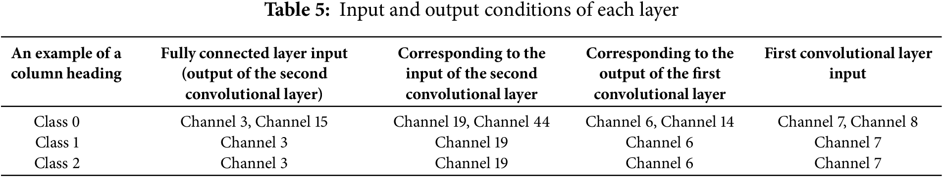
From this, it can be observed that due to the convolution kernel size of 3 and flattening, the 7th and 8th dimensions of the input to the first convolutional layer are represented by the 3rd vibration Sensor2. The data from this sensor plays a crucial role in the entire model, and its direction is radial, which is consistent with the principle of radial vibration sensitivity in practical theory when base bolts are loose. Meanwhile, from the perspective of frequency features, the distinction between Class 1 and Class 2 primarily lies in the 7th dimension. This position, within the second convolutional kernel, indicates that mid-frequency features play a more critical role in the detection of the number of loose bolts.

6  Discussion and Conclusion

This paper proposes a detection method for bolt loosening of fan base through Bayesian Learning with small dataset. It addresses the challenge of machine learning in the detection of bolt loosening, especially under the condition of small dataset. This paper presents a complete process for the detection of fan bolt loosening fault. It fully leverages the inherent advantages of Bayesian Learning, such as the ability to handle uncertainty quantification, effectively overcoming the challenges faced by conventional Deep Learning in dealing with limited datasets. After interpretability analysis, the uncertainty of the detection results and the importance of the sensors can be obtained.

The experiment is conducted using real-world fan vibration data. It not only demonstrates that the model can achieve high accuracy and robustness in real-world industrial environments for bolt loosening detection, but also utilizes Bayesian theory to quantify the uncertainty of the prediction results. However, there are several potential research directions for bolt loosening detection in industrial equipment based on Bayesian Learning that require further exploration and improvement. Future research could focus on developing dynamic or adaptive threshold adjustment strategies specifically for bolt loosening states—for example, adjusting thresholds according to the degree of loosening (e.g., slight, moderate, or severe loosening) and varying operating conditions (e.g., changes in fan load, rotational speed, or ambient vibration). This would enhance sensitivity to early-stage loosening and accuracy in distinguishing between different loosening levels in practical applications. Additionally, regarding model interpretability, although this paper has initiated an analysis of the influence of features on bolt loosening detection, there is a need for deeper and more detailed cross-layer interpretability investigations. For example, through interpretability, we can clarify which specific signal features (such as peak values in time-domain vibration, characteristic frequencies in frequency-domain analysis) are most critical for identifying bolt loosening. This would provide more intuitive explanations for why the model classifies a bolt as “loose” or “tight,” helping engineers understand and trust the detection results in industrial settings. Detection methods with small dataset still warrant further discussion and optimization. For example, small datasets in bolt loosening scenarios are often limited by scarce samples of rare loosening states or diverse bolt specifications (e.g., different bolt sizes, materials, or installation torques). Future work could explore transfer learning to adapt models to bolt loosening detection across different fan types or bolt specification.

These improvements would not only enhance model performance in bolt loosening detection but also lay the groundwork for smarter, more transparent, and reliable bolt health management. Bayesian Learning showcase promising application potential in the realm of industrial equipment fault detection. With continuous advancements in algorithm optimization and data processing technologies, this method is poised to significantly improve the accuracy and reliability of equipment fault detection, thereby providing a solid technical foundation for the transition towards highly automated, adaptive, and predictive maintenance in the industrial sector.

Acknowledgement: Not applicable.

Funding Statement: This research was funded by the Zhejiang Provincial Key Science and Technology “LingYan” Project Foundation, grant number 2023C01145; and Zhejiang Gongshang University Higher Education Research Projects, grant number Xgy22028.

Author Contributions: The authors confirm contribution to the paper as follows: Conceptualization, Haiyang Hu; methodology, Zhongyun Tang; software, Hanyi Xu; validation, Zhongyun Tang and Haiyang Hu; formal analysis, Zhongyun Tang; data curation, Zhongyun Tang and Hanyi Xu; writing—original draft preparation, Zhongyun Tang; writing—review and editing, Haiyang Hu. All authors reviewed the results and approved the final version of the manuscript.

Availability of Data and Materials: The data that support the findings of this study are available from the corresponding author, Haiyang Hu, upon reasonable request.

Ethics Approval: Not applicable.

Conflicts of Interest: The authors declare no conflicts of interest to report regarding the present study.

References

1. Molina RIR, Ruiz MJS, Molina RJR, Raby NDL, Severino-González P. Innovation systems in industry 5.0: theoretical and methodological bases. Procedia Comput Sci. 2024;231(33):595–600. doi:10.1016/j.procs.2023.12.256. [Google Scholar] [CrossRef]

2. Mon BF, Hayajneh M, Ali NA, Ullah F, Ullah H, Alkobaisi S. Digital twins in the IIoT: current practices and future directions toward industry 5.0. Comput Mater Contin. 2025;83(3):3675–712. doi:10.32604/cmc.2025.061411. [Google Scholar] [CrossRef]

3. Ramírez-Sanz JM, Maestro-Prieto J-A, Arnaiz-González Á, Bustillo A. Semi-supervised learning for industrial fault detection and diagnosis: a systemic review. ISA Trans. 2023;143(21):255–70. doi:10.1016/j.isatra.2023.09.027. [Google Scholar] [PubMed] [CrossRef]

4. Song YJ, Li SZ. Leak detection for galvanized steel pipes due to loosening of screw thread connections based on acoustic emission and neural networks. J Vibrat Cont. 2018;24(18):4122–9. doi:10.1177/1077546317720319. [Google Scholar] [CrossRef]

5. Zhou J, Chen Z, Du M, Chen L, Yu S, Chen G, et al. RobustECD: enhancement of network structure for robust community detection. IEEE Trans Knowl Data Eng. 2023;35(1):842–56. doi:10.1109/tkde.2021.3088844. [Google Scholar] [CrossRef]

6. Chen R, Chen S, Yang L, Wang J, Xu X, Luo T. Looseness diagnosis method for connecting bolt of fan foundation based on sensitive mixed-domain features of excitation-response and manifold learning. Neurocomputing. 2017;219:376–88. doi:10.1016/j.neucom.2016.09.041. [Google Scholar] [CrossRef]

7. Zheng W, Pu W, Xuejin G, Yachao Z. Fan fault diagnosis based on wavelet spectral analysis. In: Proceedings of the 2015 34th Chinese Control Conference (CCC); 2015 Jul 28–30; Hangzhou, China. doi:10.1109/chicc.2015.7260375. [Google Scholar] [CrossRef]

8. Dong ZF, Cheng H, Yang HJ, Fu W, Chen JW, Shi ZY, et al. Gearbox fault diagnosis using vibration signal with wavelet de-noising. Appl Mech Mat. 2011;86:735–8. doi:10.4028/www.scientific.net/AMM.86.735. [Google Scholar] [CrossRef]

9. van den Hoogen J, Hudson D, Bloemheuvel S, Atzmueller M. Hyperparameter analysis of wide-kernel CNN architectures in industrial fault detection: an exploratory study. Int J Data Sci Analyt. 2024;18(4):423–44. doi:10.1007/s41060-023-00440-6. [Google Scholar] [CrossRef]

10. Jiang W, Hong Y, Zhou B, He X, Cheng C. A GAN-based anomaly detection approach for imbalanced industrial time series. IEEE Access. 2019;7:143608–19. doi:10.1109/ACCESS.2019.2944689. [Google Scholar] [CrossRef]

11. Zhou J, Xie C, Gong S, Wen Z, Zhao X, Xuan Q, et al. Data augmentation on graphs: a technical survey. ACM Comput Surv. 2025;57(11):1–34. [Google Scholar]

12. Zhou J, Hu C, Chi J, Wu J, Shen M, Xuan Q. Behavior-aware account de-anonymization on ethereum interaction graph. IEEE Trans Inform Foren Secur. 2022;17:3433–48. doi:10.1109/tifs.2022.3208471. [Google Scholar] [CrossRef]

13. Pearl J. Chapter 2—Bayesian inference. In: Pearl J, editor. Probabilistic reasoning in intelligent systems. San Francisco, CA, USA: Morgan Kaufmann; 1988. p. 29–75. doi:10.1016/B978-0-08-051489-5.50008-4. [Google Scholar] [CrossRef]

14. Goan E, Fookes C. Bayesian neural networks: an introduction and survey. In: Mengersen KL, Pudlo P, Robert CP, editors. Case studies in applied bayesian data science: CIRM Jean-Morlet Chair, Fall 2018. Cham, Switzerland: Springer International Publishing; 2020. p. 45–87. doi:10.1007/978-3-030-42553-1_3. [Google Scholar] [CrossRef]

15. Zhang X, Zou Y, Li S. Bayesian neural network with efficient priors for online quality prediction. Digit Chem Eng. 2022;2(4):100008. doi:10.1016/j.dche.2021.100008. [Google Scholar] [CrossRef]

16. Dilawar M, Shahbaz M. A bayesian optimized stacked long short-term memory framework for real-time predictive condition monitoring of heavy-duty industrial motors. Comput Mater Contin. 2025;83(3):5091–114. doi:10.32604/cmc.2025.064090. [Google Scholar] [CrossRef]

17. Neal RM. Monte carlo implementation of gaussian process models for bayesian regression and classification [Internet]. [cited 2025 Aug 1]. Available from: https://arxiv.org/pdf/physics/9701026. [Google Scholar]

18. Gal Y, Ghahramani Z. Dropout as a bayesian approximation: representing model uncertainty in deep learning. In: Proceedings of the International Conference on Machine Learning; 2016 Jun 19–24; New York, NY, USA. [Google Scholar]

19. Chen H, Ren L. ACO-GCN: a fault detection fusion algorithm for wireless sensor network nodes. Int J Ind Eng Theory Appl Pract. 2023;30(2):337–49. doi:10.23055/ijietap.2023.30.2.8801. [Google Scholar] [CrossRef]

20. Clare MCA, Sonnewald M, Lguensat R, Deshayes J, Balaji V. Explainable artificial intelligence for bayesian neural networks: towards trustworthy predictions of ocean dynamics. J Adv Model Earth Syst. 2022;14(11):e2022MS003162. doi:10.1029/2022ms003162. [Google Scholar] [CrossRef]

21. Mihaljević B, Bielza C, Larrañaga P. Bayesian networks for interpretable machine learning and optimization. Neurocomputing. 2021;456:648–65. doi:10.1016/j.neucom.2021.01.138. [Google Scholar] [CrossRef]

22. Zhou J, Gong S, Chen X, Xie C, Yu S, Xuan Q, et al. Clarify confused nodes via separated learning. IEEE Trans Pattern Analy Mach Intelli. 2025;47(4):2882–96. doi:10.1109/tpami.2025.3528738. [Google Scholar] [PubMed] [CrossRef]

23. Luo J, Li K, Xie C, Yan Z, Li F, Jia X, et al. A novel anti-loosening bolt looseness diagnosis of bolt connections using a vision-based technique. Sci Rep. 2024;14(1):11441. doi:10.1038/s41598-024-62560-8. [Google Scholar] [PubMed] [CrossRef]

24. Nguyen T-T, Ta Q-B, Ho D-D, Kim J-T, Huynh T-C. A method for automated bolt-loosening monitoring and assessment using impedance technique and deep learning. Develop Built Environ. 2023;14(6):100122. doi:10.1016/j.dibe.2023.100122. [Google Scholar] [CrossRef]

25. Sui X, Duan Y, Yun C, Tang Z, Chen J, Shi D, et al. Bolt looseness detection and localization using wave energy transmission ratios and neural network technique. J Infrastruct Intelli Resil. 2023;2(1):100025. doi:10.1016/j.iintel.2022.100025. [Google Scholar] [CrossRef]

26. Hu YJ, Guo WG, Jiang C, Zhou YL, Zhu W. Looseness localization for bolted joints using Bayesian operational modal analysis and modal strain energy. Adv Mech Eng. 2018;10(11):1687814018808698. doi:10.1177/1687814018808698. [Google Scholar] [CrossRef]

27. Zhou T, Han T, Droguett EL. Towards trustworthy machine fault diagnosis: a probabilistic Bayesian deep learning framework. Reliab Eng Syst Saf. 2022;224(2):108525. doi:10.1016/j.ress.2022.108525. [Google Scholar] [CrossRef]

28. Zhou T, Zhang L, Han T, Droguett EL, Mosleh A, Chan FTS. An uncertainty-informed framework for trustworthy fault diagnosis in safety-critical applications. Reliab Eng Syst Saf. 2023;229(8):108865. doi:10.1016/j.ress.2022.108865. [Google Scholar] [CrossRef]

29. Li H, Jiao J, Liu Z, Lin J, Zhang T, Liu H. Trustworthy Bayesian deep learning framework for uncertainty quantification and confidence calibration: application in machinery fault diagnosis. Reliab Eng Syst Saf. 2025;255:110657. doi:10.1016/j.ress.2024.110657. [Google Scholar] [CrossRef]

30. Yao Y, Han T, Yu J, Xie M. Uncertainty-aware deep learning for reliable health monitoring in safety-critical energy systems. Energy. 2024;291(4):130419. doi:10.1016/j.energy.2024.130419. [Google Scholar] [CrossRef]

31. Chen D, Xie Z, Liu R, Yu W, Hu Q, Li X, et al. Bayesian hierarchical graph neural networks with uncertainty feedback for trustworthy fault diagnosis of industrial processes. IEEE Trans Neu Netw Learn Syst. 2024;35(12):18635–48. doi:10.1109/tnnls.2023.3319468. [Google Scholar] [PubMed] [CrossRef]

32. Winkler L, Ojeda C, Opper M. Stochastic control for bayesian neural network training. Entropy. 2022;24(8):1097. doi:10.3390/e24081097. [Google Scholar] [PubMed] [CrossRef]

33. Blundell C, Cornebise J, Kavukcuoglu K, Wierstra D. Weight uncertainty in neural networks. In: Proceedings of the 32nd International Conference on International Conference on Machine Learning; 2015 Jul 3–11; Lille, France. p. 1613–22. [Google Scholar]

34. Bai G, Chandra R. Gradient boosting Bayesian neural networks via Langevin MCMC. Neurocomputing. 2023;558(4):126726. doi:10.1016/j.neucom.2023.126726. [Google Scholar] [CrossRef]

35. Mostafa B, Hassan R, Mohammed H, Tawfik M. A review of variational inference for bayesian neural network. Artif Intell Indust Applicat. 2023;21:231–43. doi:10.1007/978-3-031-43520-1_20. [Google Scholar] [CrossRef]

36. Deep universal probabilistic programming. [Internet]. [cited 2025 Aug 1]. Available from: https://pyro.ai/. [Google Scholar]