Research on Vehicle Joint Radar Communication Resource Optimization Method Based on GNN-DRL

1  Introduction

In intelligent transportation systems (ITS), the demand for real-time performance in vehicle environmental perception and vehicle-to-everything (V2X) communication is growing rapidly—meanwhile, with the development of autonomous driving technology, efficient transmission and processing of massive data from vehicle sensors (e.g., radar, cameras) has become a research focus. Although JRC technology provides a new approach by enabling radar-communication collaboration in a shared frequency band [1–3], its traditional resource allocation (including early fixed solutions like hardware design and time-division multiplexing [4–6]) all relies on static optimization or predefined rules, making it difficult to address instantaneous interference and multi-agent collaboration in dynamic traffic environments. While DRL offers an adaptive solution, its collaborative efficiency and information exchange capabilities are insufficient in some scenarios, thus creating an urgent need for an intelligent resource allocation framework that can efficiently process dynamic graph structures and optimize multi-agent collaboration.

In resource allocation research, traditional convex optimization, greedy algorithms, and static AoI optimization models are widely used but limited by reliance on prior channel parameters or inability to cope with environmental transients [7–10]. In multi-agent collaboration, centralized control lacks scalability due to high overhead, while fixed clustering algorithms lack dynamic learning capabilities [11,12]. In recent years, DRL has become a focus for its adaptability to dynamic environments: single-agent methods (e.g., Deep Q-Network (DQN), Deep Deterministic Policy Gradient (DDPG) [13,14]) handle action spaces, and multi-agent methods (e.g., centralized DDPG [15,16]) achieve strategy sharing, yet they still face limitations like single action spaces and insufficient environment modeling [17,18].

As the demand for real-time performance in intelligent transportation systems increases, researchers have begun to explore the integration of DRL and GNN. GNNs model node interactions through graph structures, demonstrating advantages in multi-agent collaboration. For example, Reference [19] uses GCNs to optimize information aggregation, while Reference [20] combines GraphSAGE to achieve dynamic neighbor selection, both of which effectively improve resource allocation efficiency. In addition, Hieu et al. (2022) proposed a joint radar-data communication framework for self-driving vehicles based on relocatable deep reinforcement learning, which significantly improves cross-environmental adaptation [21]. Sohaib et al. (2024), on the other hand, implemented energy-efficient resource allocation in V2X communication through dynamic meta-migration learning, which further enhances the robustness of the system in dynamic environments [22].

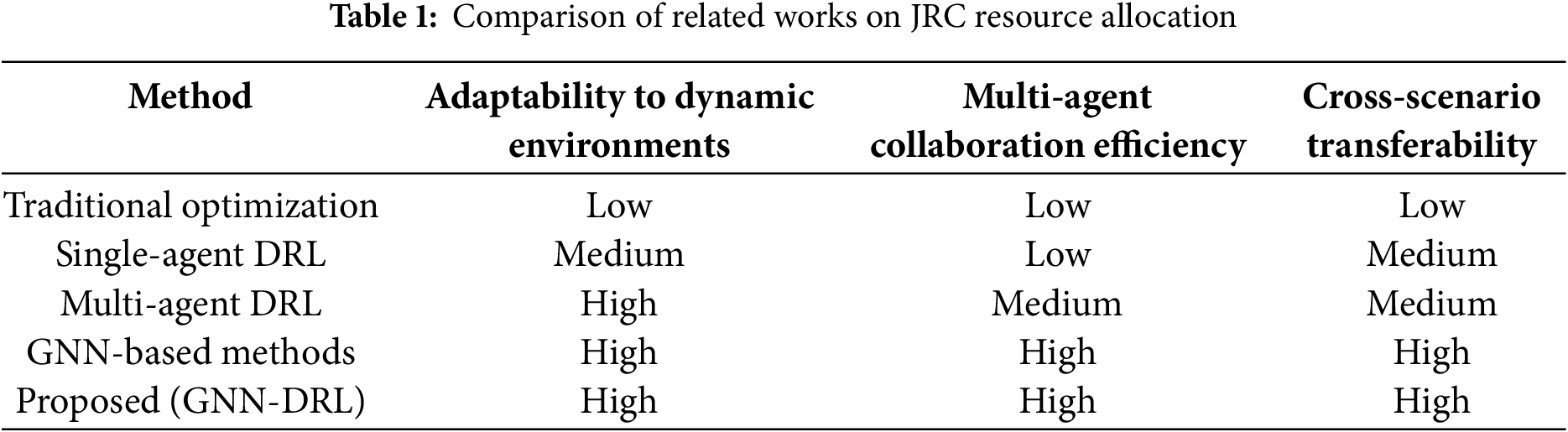
For JRC performance optimization, researchers focus on AoI and communication success rates. Ref. [23] minimizes drone-assisted network AoI via MAPPO, while Ref. [24] uses a weighted reward function to balance radar-communication efficiency. Notably, radar interference in millimeter-wave communications drives dynamic resource scheduling algorithm development: Ref. [25] proposes a DRL-based anti-interference strategy, and Ref. [26] enhances system robustness via joint trajectory-data scheduling optimization. However, existing research has three key challenges: poor resource allocation adaptability in dynamic environments, low multi-agent collaborative info exchange efficiency, and no cross-scenario transferability [27]. Table 1 compares five typical JRC resource allocation methods (Traditional Optimization, Single-agent DRL, Multi-agent DRL, GNN-based methods, and the proposed GNN-DRL) in the three challenge-related dimensions (adaptability to dynamic environments, multi-agent collaboration efficiency, cross-scenario transferability), showing only the proposed GNN-DRL achieves “High” in all dimensions.

Existing research still faces three major challenges: insufficient adaptability in resource allocation within dynamic environments; inefficient information exchange during multi-agent collaboration; and a lack of cross-scenario generalization capabilities. To address these challenges, this study proposes an intelligent resource optimization framework that integrates GNN with MADRL. This framework models the problem as a Partially Observable Markov Game (POMG), introduces a weighted reward function to balance radar and communication tasks, and employs GCN and GraphSAGE to enable efficient information exchange among agents. The main contributions of this paper are as follows: A novel GNN-DRL fusion architecture for dynamic JRC resource allocation is proposed. A weighted reward mechanism balancing AoI and Signal to Interference plus Noise Ratio (SINR) objectives is designed.

2  Research on Joint Radar Communication Resource Allocation in a Two-Lane Scenario

2.1 Two-Lane Model

Consider a vehicular system that contains a number N of vehicles (Fig. 1) that travel along a two-lane roadway. In real traffic scenarios, lanes and vehicle speeds are correlated. This model assumes uniform speed per lane, with outer lanes having relatively higher speeds, which aligns with common traffic flow patterns. Each vehicle has four directional antennas for short-range radar detection and a data transceiver that works in four basic directions. Over time, vehicles collect data via their sensor systems and store it in memory. At each discrete time step, a vehicle must decide: transmit sensor data or conduct radar detection. If choosing communication, it further determines which stored data to send and the transmission direction. This decision simulates vehicles’ dynamic resource allocation in real scenarios.

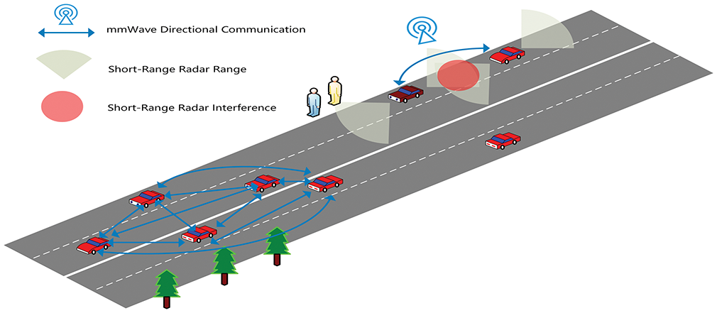
Figure 1: Two-lane model

2.2 Interference with Radar and Communication Systems and Countermeasures

In real scenarios, surrounding vehicles’ radar subsystems usually operate independently at regular intervals, potentially interfering with the target vehicle’s millimeter-wave communications. To address this, intelligent vehicles in this study have learning capabilities, enabling them to arrange radar and communication operations based on their environment. They can monitor surrounding radar signal characteristics (e.g., intensity, frequency) and adjust their radar detection intervals or communication bands to reduce interference impact. When strong surrounding radar interference is detected, they may temporarily delay communication to prioritize radar detection (ensuring accurate environmental perception) or choose less interfering bands to improve communication success rates.

2.3 Communication Access Solutions in Multi-Agent Scenarios

In multi-agent scenarios, vehicles coordinate sensor data transmission through narrowband control channels using a shared channel competition mechanism. Vehicles compete for access to shared communication channels and combine graph neural networks with dynamic neighbor selection and attention mechanisms to optimize resource allocation. In this case, vehicles need to allocate resources more intelligently to avoid communication conflicts and improve communication efficiency.

2.4 Mathematical Expression and Implementation Approach of System Objectives

Vehicles in the JRC system must decide when to conduct radar detection to get accurate speed info of surrounding objects—critical for autonomous driving safety. In complex traffic, knowing surrounding vehicle speeds aids timely collision-avoidance decisions. They can predict and transmit the most valuable current data, choose optimal transmission directions for needy vehicles, and select best communication time steps to maximize SINR, boosting transmission success and throughput. These goals are mathematically integrated into the subsequent POMG model to quantify and optimize vehicle decisions.

3  Establish a POMG Model

In the JRC system, each intelligent vehicle is considered as an intelligence, and the multi-agent JRC problem is defined as a POMG since each agent can only obtain local observations and cannot know the observations or actions of other agents. At each discrete time step t, agent i makes observations of its local state and environmental conditions oi, while the complete state of the whole system s is formed by concatenating the observations of all N agents, i.e., s=[o1,o2,…,oN]. Based on oi, agent i decides how to operate its communication or radar system via a stochastic policy π:O→P(A) (e.g., selecting the radar detection action aradar or communication action (ad,aθ)), where O is the observation space and A is the action space. The environment then updates s according to the state transition model (accounting for data age growth, vehicle movement, and communication channel characteristics), and agent i receives a reward ri based on the reward function R:S×A→R—this reward function is designed to guide agents toward the system objectives outlined in Section 2.4. Below, the observation space, action space, state transition model, and reward function of the POMG are defined in detail.

3.1 Observation

Observations of this vehicle oi consist of multiple features describing the local environmental conditions, the configuration of the surrounding vehicles, and the accumulated sensing data of this vehicle, defined as:

o=[α,e,x,v,d,dθ],(1)

where α denotes the time step (i.e., the number of time steps that have elapsed since the last radar detection was performed) since the last radar information was collected on this vehicle; the environmental vector e=[w,m,v] contains three environmental state features indicating the necessity of radar detection at the current time step: w represents weather conditions (0=clear, 1=rainy, 2=foggy), m indicates the presence of nearby moving objects (0=absent, 1=present), and v is the speed of the vehicle. Each environmental feature is graded within an integer set {w,m,v}∈{0,1,…,Emax}, where Emax=2 (the maximum grade of environmental features, with 0 representing the safest condition), and v∈RN−1 (where N is the total number of vehicles), higher values indicate higher risk; the vectors x∈R2(N−1) and represent the position and speed of the other N−1 vehicles relative to the vehicle. Position is two-dimensional, located in the plane of the roadway, and consists of distance along the longitudinal direction of the roadway and lane position in the transverse direction; speed is one-dimensional, and consists of a velocity component along the direction of the roadway only, as the vehicle is traveling along a straight roadway, and is obtained by the vehicle through direct measurements of odometer sensors of neighboring vehicles and by a GNSS system. These values, position and speed can be corroborated by sensor fusion when sensed data are available; features d and dθ denote scalar fields (discretized in the spatial domain) of available sensing data stored in the vehicle’s memory, represented as a 2D array whose origin corresponds to the vehicle’s instantaneous position: d∈RA×B, where A=20 (number of discrete grid points along the roadway’s longitudinal direction) and B=4 (number of discrete grid points along the roadway’s lateral direction), represents the Age of Information (AoI) of sensing data corresponding to vehicle positions. Data exceeding the maximum aging threshold αmax=30 (a pre-defined invalid data threshold; data beyond this value is deemed outdated and deleted) is discarded, so the array element dab∈[0,αmax]; dθ describes the azimuth of each data point relative to the vehicle’s traveling direction at the time of collection, discretized based on the vehicle’s direction as dθ,ab∈{F,R,B,L,null}=Dθ∪null, where F (front), R (right), B (rear), and L (left) denote directions, and null indicates no data at coordinates (a,b).

3.2 Actions

3.2.1 Motion Space Definition

The set of actions A contains several different decision options. Among them is the action aradar to perform radar detection, where the radar subsystem acquires real-time velocity information about the surrounding objects, and the system tends to choose the radar action when environmental characteristics indicate the need for more frequent sensing. There is also the communication action (ad,aθ) for data transmission, where the data selection ad corresponds to the discrete data orientation state dθ, and the vehicle transmits data matching dθ and ad in memory. The transmission direction aθ selects the physical direction of the communication antenna to ensure that the data is sent to the target vehicle. The direction selection takes into account the relative position of the receiving vehicle and the SINR of the communication link. in addition an empty action is included to indicate that the smart body does not perform any new action at the current time step, keeping the existing policy unchanged.

The whole set of actions can be represented as:

A={(ad,aθ)|ad∈Ad,aθ∈Aθ}∪{(aradar,null)}.(2)

3.2.2 Data Transmission Rules

If the agent selects the communication action (ad,aθ), it first needs to filter the sensing data in its memory whose azimuth matches ad based on the data azimuth matrix dθ, ensuring the transmitted data meets the requirements of the target direction. The final data to be sent, d<send>, is determined jointly by the indicator function 1ad(dθ) (which filters data with matching azimuth) and the Hadamard product (which associates with the timeliness of the data AoI matrix d):

d<send>=1ad(dθ)∘d,(3)

where 1ad(⋅) is the indicator function, which serves to accurately filter the data whose azimuth angle matches the target transmission direction ad. ∘ is the Hadamard product (multiplication of elements). It is the element-by-element multiplication operation of the data retained after screening by the indicator function with the AoI corresponding to that data.

The data of the vehicle j that receives the data update is shifted according to the position of the vehicle i that sends it:

dj⟨rec⟩(x1,x2)=di⟨send⟩(x1+x1,ji,x2+x2,ji),(4)

where x1,ji and x2,ji are the positional offsets of vehicle j with respect to i.

3.3 State Transition Model

The state transition model describes each vehicle’s observation changes in subsequent time steps based on all vehicles’ current observations and actions, and vehicle actions’ effect on the wireless channel. When time advances to the next step, each vehicle’s data age increases by 1, and data features shift with its travel distance due to movement. Vehicles may get new data via their sensors or from neighbors, both updating their states. The data age formula is as follows:

dt+1(x1,x2)=min(dt(x1+vtΔt,x2)+1,αmax),(5)

where dt(x1+vtΔt,x2)+1 indicates that as time advances fromt to t+1 (interval Δt), the data age is naturally incremented by 1 from the original position after updating. Use the min function, it is ensured that the data age at the time of t+1 does not exceed the maximum threshold αmax.

During the communication process, factors such as the power and signal-to-noise ratio (SINR) of the signal transmission play a key role in the transmission effect, which in turn affects the state transfer. When the transmitted signal reaches the target vehicle j, the received power Pij is given by:

Pij=GiGjLijPi,(6)

where Pi is the transmitted power, Gi and Gj are the antenna gains of the transmitting and receiving vehicles, respectively, and Lij is the path loss, which is related to factors such as the distance between vehicles. Based on the received power, the signal to noise ratio is calculated:

SINRij=Pij∑k∈𝒩∖iσk+nj,(7)

where ∑k∈𝒩∖iσk is the radar interference generated by other vehicles and nj is the background noise. If the SINR meets certain conditions, data transmission is successful, and the vehicle status changes due to receiving new data; if transmission fails, the vehicle may readjust its transmission strategy, retry transmission, or select other actions, reflecting the dynamic interaction between the vehicle and its environment.

3.4 Reward

The reward function r(t) is the core mechanism to guide the vehicle’s decision making, including communication reward and radar reward, which balances the importance of radar detection and communication by weighted summation to encourage the vehicle to make decisions that meet the system goals. The reward function is represented as:

r(t)=wcomm(rSINR×rdata)+wradarrradar,(8)

where wcomm and wradar are weights to adjust the relative importance of communication and radar functions in decision making. In different driving scenarios, these weights can be adjusted to optimize the system performance according to the actual needs. rSINR aims to encourage vehicles to maximize data transmission SINR at the expected receiver by calculating the sum of transmission success rates ηij for all receiving vehicles, i.e.,

rSINR=∑j∈𝒩∖iηij,(9)

a higher SINR means that data transmission is more reliable and can deliver information to other vehicles more efficiently. rdata encourages vehicles to send data that is more useful to other vehicles, with calculations that take into account the receiving vehicle’s priority for different location data and the age of the data. The specific calculations are:

rdata=∑j∈𝒩∖ivj(∑a,b(Wj)ab∘max(0,αmax−(dj<rec>)ab)),(10)

where (Wj)ab denotes the importance weight of the receiving vehicle j for data at position (a,b) (element of the position weight matrix), which is related to the vehicle’s traveling direction and safety needs—for example, the vehicle assigns a weight of 1.2 to data in front of or near its own position, and 0.6 to data behind or far from its position; vj is associated with the individual state of vehicle j (e.g., vj=1.5 for high-speed travel, vj=0.8 for low-speed travel), reflecting the urgency of its demand for environmental perception information. rradar is used to encourage vehicles to perform radar detection when necessary, and when a non-radar detection action is selected, a corresponding penalty will be given according to the environmental conditions and the time of the last radar detection. The specific formula is:

rradar=−1a≠aradar(exp⁡(eβ)×f(α)),(11)

where 1a≠aradar is an indicator function, used to determine whether the current action is a radar detection action; β is a coefficient vector, used to adjust the degree of influence of environmental conditions on the punishment; f(α) is a non-decreasing function on α, often taken as f(α)=1Z+(α) in the experiment, which means that with the increase in the interval of the last radar detection time α, the punishment will be increased accordingly to motivate the vehicle to carry out radar detection in time, in order to ensure an accurate perception of the surrounding environment.

4  Deep Reinforcement Learning Algorithms

For multi-agent problems, the MAPPO algorithm is proposed, which achieves distributed decision-making and knowledge sharing by randomly assigning strategies to agents [28].

This algorithm is a strategy optimization algorithm suitable for multi-agent systems and plays an important role in JRC problems. Its core principle is to maximize the expected reward of agents by optimizing strategies, while considering the interaction and coordination between multiple agents.

4.1 Strategy Representation and Optimization Objectives in Multi-Agent Systems

The goal of reinforcement learning is to learn an optimal strategy that allows the intelligent agent to obtain the maximum expected cumulative reward in the system [29]. For a single intelligent body, its expected reward can be expressed as:

J(πi)=Es∼Prπi,ai∼πi[∑t=1∞γt−1ri,t],(12)

where Prπi is the probability distribution of the state under the strategy πi, γ is the discount factor, and ri,t is the reward obtained by the intelligent body i at time step t.

4.2 Loss Function in the MAPPO Algorithm

The MAPPO algorithm updates strategy parameters by optimizing the loss function and uses a clipped proxy objective function to limit the step size of strategy updates in order to improve the stability of the algorithm. For the detailed derivation process of the CLIP loss function, please refer to Appendix A. For the kth policy πk, in a multi-intelligent body system its clip loss function LCLIP(θk) is:

LCLIP(θk)=Eoi,ai∼πk[min(ρt(θk)A^iπk(t),max(1−ε,min(ρt(θk),1+ε))A^iπk(t))],(13)

where ρt(θk)=πk(at|ot)πk,old(at|ot) denotes the probability ratio between the current strategy πk and the last updated strategy πk,old at time step t, and ε is a hyperparameter to control the magnitude of the strategy update. A^iπk(t) is the estimated dominance value of the intelligencei at time stept under the strategy πk, computed as:

A^iπk(s,a)≈r(s,a)+γV^iπk(s(t+1))−V^iπk(s(t)),(14)

where r(s,a) is the immediate reward obtained by the intelligent in states for taking actiona and V^iπk is the value network’s estimate of the value of the intelligent agent i state under strategy πk.

4.3 Updating the Value Network

In addition to optimizing the policy network, the MAPPO algorithm also involves updating the value network. The value network is used to estimate the value of agents in different states, helping the policy network to better evaluate the merits of actions. The parameters of the value network ϕk are updated by minimizing the mean square error loss, and the loss function LVAL(ϕk) is:

LVAL(ϕk)=Eoi,ai∼πk[(V^iπk(oi(t))−y(t))2],(15)

where the objective value, y(t)=r(t)+γV^iπk(s(t+1)), combines the immediate reward r(t), with an estimate of the value of the next state. By minimizing the mean square error loss, the estimate of the value network is made closer to the true value, thus assisting the strategy network to make better decisions.

4.4 Entropy Reward Term

In order to promote the exploration of state-action space by intelligences, the MAPPO algorithm also introduces an entropy reward term S[πψk](o). The overall objective function becomes:

LCLIP+VAL(ψk)=Et[LCLIP(ψk)−k1LVAL(ϕk)+k2S[πψk](o)],(16)

where k1 and k2 are coefficients used to balance the weights between strategy loss, value loss and entropy reward. The entropy reward encourages the intelligent agent to try different actions and avoid converging too early on a local optimal strategy.

4.5 Algorithm Execution Process

During the execution of the MAPPO algorithm, each intelligent body chooses an action based on its current strategy πiai and interacts with the environment to obtain a reward ri and the next observation oi,t+1. Then, use the collected experience data to calculate the loss function and update the parameters of the policy network and value network through the gradient descent algorithm. Repeat this process until the algorithm converges or reaches the predetermined stopping condition.

5  Graph Neural Networks

In the resource allocation problem of multi-agent JRC systems, GNN exhibits significant advantages—traditional methods struggle to handle complex dynamic graph structures and multi-agent interactions, while GNN can effectively capture node relationships and information propagation rules. During the execution of the MAPPO algorithm, each agent first fuses its local observation oi with neighbor information via this framework. Then, based on the policy network πi that takes the fused features as input, the agent selects an action ai (e.g., radar detection aradar or communication action (ad,aθ)) from the action space defined in Section 3.2, and interacts with the JRC environment to obtain a reward ri and the next local observation oi,t+1; oi,t+1 is also processed through this GNN framework. Fig. 2 shows the overall structure of this intelligent optimization framework, which takes local vehicle environmental observations as input, processes them via the hierarchical GNN, and finally generates collaborative decisions through the MAPPO algorithm.

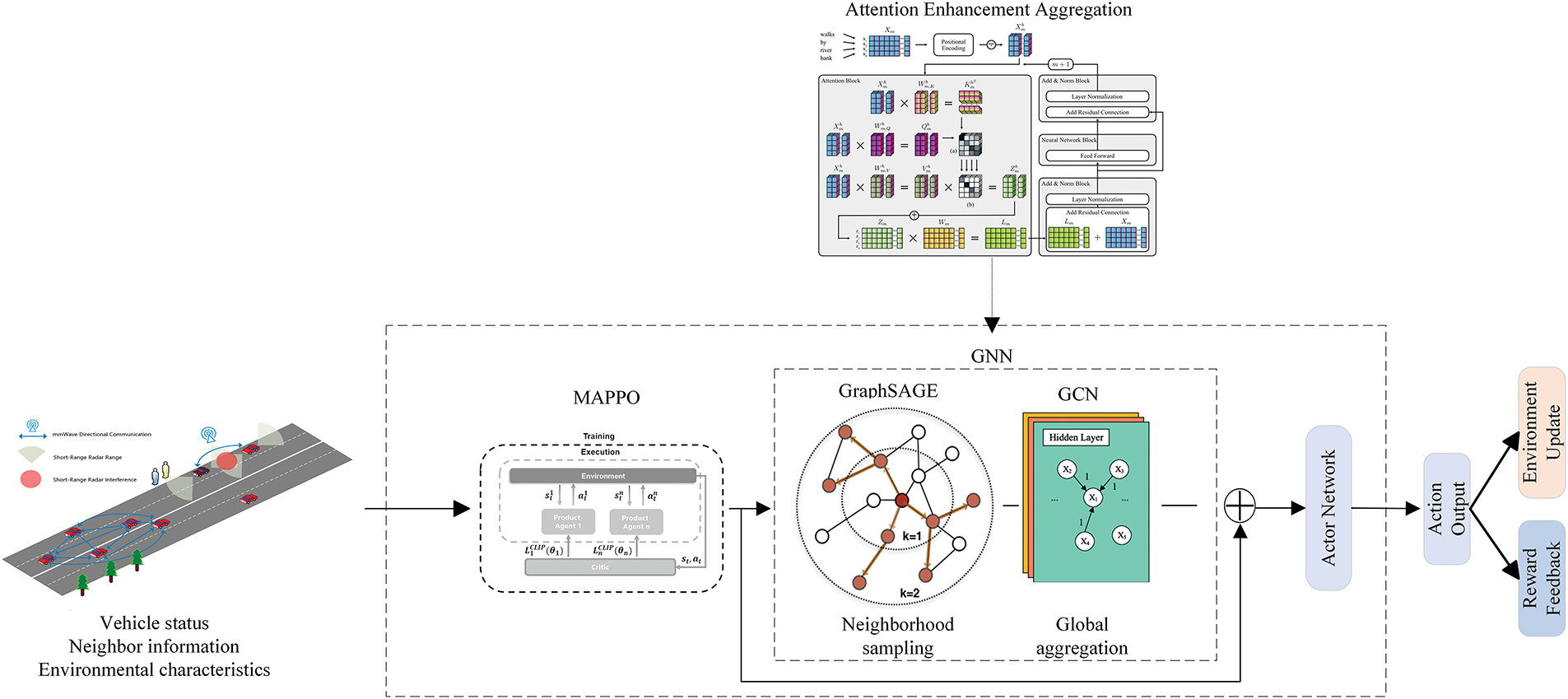
Figure 2: Structure of a vehicle JRC resource allocation model based on graph neural networks

5.1 Principles of GraphSAGE

GraphSAGE is an inductive graph neural network that updates the features of target nodes by sampling and aggregating the features of neighboring nodes.

Sampling Neighbor Nodes: sampling a fixed number S of neighbor nodes from the set 𝒩(i) of neighbors of nodei, denoted as 𝒩S(i).

Aggregate neighbor features: taking mean value aggregation as an example, the feature update formula for node i at layer l is:

h𝒩(i)(l)=MEAN({hj(l),∀j∈𝒩S(i)}),(17)

hi(l+1)=σ(W1(l)hi(l)+W2(l)h𝒩(i)(l)),(18)

where W1(l) and W2(l) are the learnable weight matrices and σ is the activation function. GraphSAGE can adapt to dynamic graph structures, but may ignore long-range dependencies.

5.2 Principles of GCN

GCN aggregates and transforms the features of nodes during message passing. Suppose the graph G=(V,E), where V is a collection of nodes and E is a collection of edges. The feature vector of nodei at layer l is hi(l), the adjacency matrix is A, the degree matrix is D and the learnable weight matrix is W(l). First, add the self-loop to get A^=A+I, where I is the unit matrix. Then calculate the degree matrix D^, D^ii=∑j=0NA^ij corresponding to A^. The update formula is:

hi(l+1)=σ(D^−12A^D^−12hi(l)W(l)),(19)

where σ is the activation function ReLU. GCN can effectively capture the global structural information of the graph, but may have some limitations when dealing with dynamic graphs.

5.3 Neighbor Selection and Attention Mechanism Optimization Based on the Fusion of GraphSAGE and GCN

Based on the existing GraphSAGE neighbor sampling, dynamic weights and attention mechanisms are introduced to improve the specificity of information aggregation.

5.3.1 Dynamic Adjacency Weight

Weights based on interference intensity are added to the aggregation function of GraphSAGE. Assuming that the distance between vehicles u and v is duv and the attenuation coefficient is λ, the aggregation formula is:

zv=σ(Wa⋅∑u∈Ns(v)Xu⋅δuv⋅exp⁡(−λduv)|Ns(v)|+ba),(20)

where δuv denotes the connection relationship (0 or 1) between nodes u and v, this formula gives priority to aggregating the information of close and high interference neighbors.

5.3.2 Attention Enhancement Aggregation

Combine the attention of GraphSAGE with the neighbor matrix of GCN. First, calculate the attention weights α:

α=Softmax(WqhiGCN+WkhiGraphSAGE),(21)

then, fuse the features of GCN and GraphSAGE:

hicomb=α⊙hiGCN+(1−α)⊙hiGraphSAGE.(22)

5.3.3 Dynamic Adjacency Weight

Propose a layered fusion framework that combines the global structural information of GCN and the local dynamic features of GraphSAGE.

Stratified aggregation

Bottom layer: GraphSAGE performs local neighbor sampling and feature aggregation to obtain local features hilocal:

hilocal=GraphSAGE(hiraw).(23)

High-level: GCN propagates the features output by GraphSAGE globally to obtain global features higlobal:

higlobal=GCN(hilocal).(24)

Concatenate local features and global features to obtain the final features hifinal:

hifinal=Concat(hilocal,higlobal).(25)

Joint decision-making

Feed the fusion features into the policy network to obtain the resource allocation probability pi:

pi=softmax(Wfinalhifinal+bfinal).(26)

As shown in Algorithm 1:

6  Experimental Evaluation

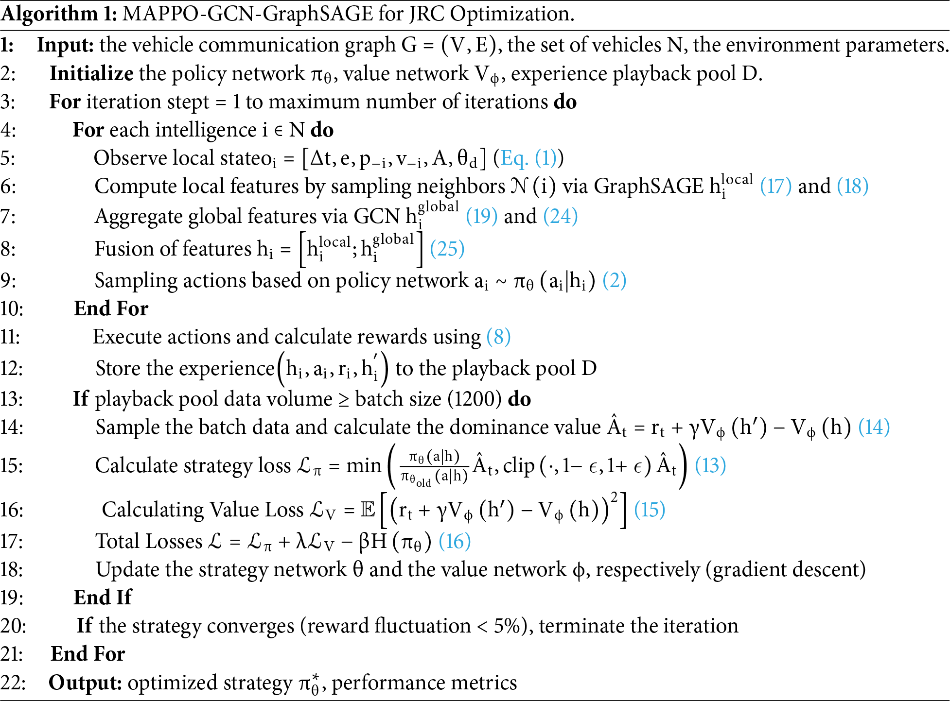
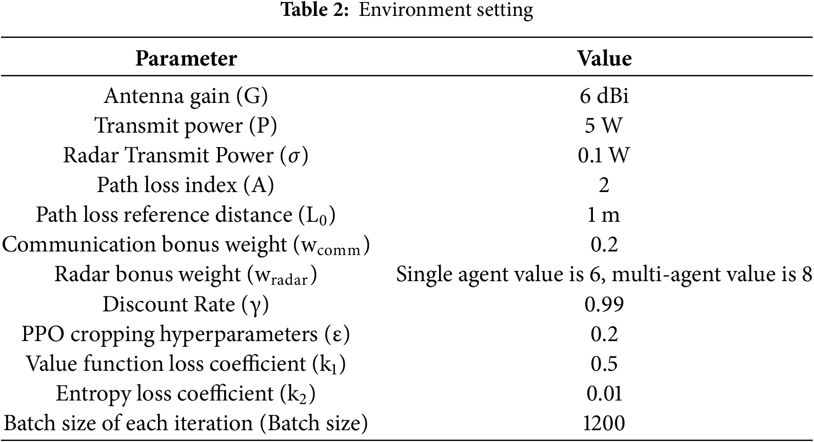
This experiment’s code was implemented with Python and the PyTorch framework, using the PyTorch Geometric library to process graph structure data for training and optimizing multi-agent collaboration strategies. It simulates a two-lane traffic scenario where the number of vehicles varies dynamically, with initial positions and velocities randomly generated to reflect real traffic uncertainty. Each vehicle has four directional antennas operating in the millimeter-wave band, supporting radar detection and directional communication. The simulation environment integrates multiple channel fading models to accurately reflect complex wireless communication propagation characteristics. Agent decision-making relies on MDP modeling, with reward functions based on SINR and AoI to guide resource allocation; radar reward weights are set differently for single-agent and multi-agent scenarios to balance radar detection and communication efficiency. At the algorithm level, the MAPPO framework is adopted, combining GCN and GraphSAGE for dynamic information exchange, and optimizing message passing via neighbor sampling and attention mechanisms. Key parameters are specified in a table to provide a standardized basis for experiment reproduction and comparison, and see Table 2 for detailed values of these parameters.

Time Division Multiplexing (TDM) allocates fixed time intervals to separate radar and communication functions, with no dynamic adjustment and independent of real-time environmental changes. It divides the time axis into periodic frames (total T time steps per frame): a dedicated segment (e.g., 30% of T, denoted t1) is for radar detection, and the remaining segment (e.g., 70% of T, denoted t2, where t1 + t2 = T) is for communication—cycling through directions like front, right, back, and left. This strict time partitioning prevents interference between radar and communication, mimicking the operation of traditional time-division systems in industrial.

Fig. 3 shows that as the number of training iterations increases, the traditional TDM method using fixed time slot allocation, due to its rigid resource allocation rules and lack of environmental adaptability, consistently maintains the lowest reward values across all curves and shows no significant room for improvement. While the SOTA algorithm maintains a high stable range for communication rewards in the later stages and shows a steady growth trend for radar rewards and average total rewards, it lacks dynamic optimization fluctuations and exhibits significant flexibility deficiencies. In contrast, the PPO algorithm demonstrates superior performance evolution with training iterations in the experiments. Communication rewards exhibit dynamic adjustment characteristics even at stable high levels, radar rewards reach a peak early on and subsequently adapt to environmental fluctuations for optimization, and average total rewards maintain higher levels in the later stages. This fully validates PPO’s ability to dynamically optimize radar and communication strategies through reinforcement learning, highlighting the significant potential of reinforcement learning algorithms in JRC tasks compared to fixed-rule TDM methods and SOTA algorithms that are stable but lack flexibility.

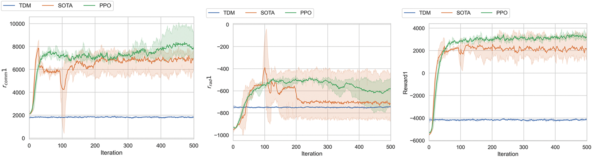
Figure 3: The communication rewards, radar rewards, and average total rewards of the traditional TDM method, SOTA algorithm and the PPO algorithm in a single-agent experiment

The left part of Fig. 4 takes “number of vehicles (5–25)” as the horizontal axis and “average total reward” as the vertical axis, comparing the performance of the PPO algorithm and the traditional TDM method through bar charts. The results show that in all scenarios with different numbers of vehicles, the average total reward of the PPO algorithm is significantly higher than that of the TDM method; even as the number of vehicles increases, the PPO algorithm can still stably maintain its reward advantage. This phenomenon verifies the efficiency of PPO in dynamic resource allocation—compared with the rigid rules of TDM’s fixed time slot allocation, PPO can flexibly adjust the resource ratio between radar and communication according to changes in the number of vehicles, better adapting to the resource demands in multi-vehicle scenarios.

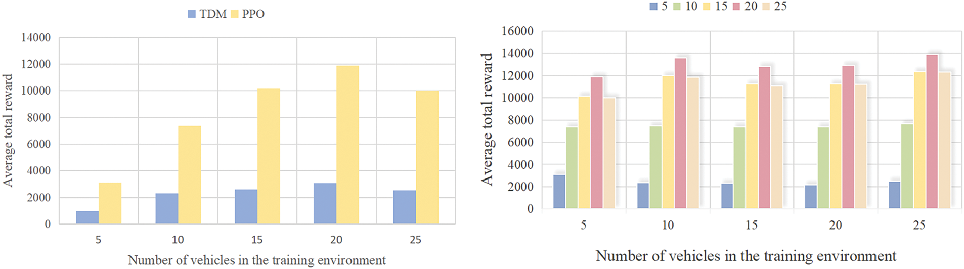
Figure 4: Average total reward of PPO and TDM algorithms under different vehicle numbers and PPO robustness analysis (Evaluation Metric: Standard Deviation of Fluctuation in Average Total Rewards)

The right part of Fig. 4 focuses on the “difference in the number of vehicles between the training and testing environments” and reflects the robustness of the PPO algorithm (with the evaluation metric being the standard deviation of fluctuation in the average total reward) through the height variation of the bar charts. When the number of vehicles in the testing environment is consistent with or close to that in the training environment, the PPO algorithm achieves the highest reward value; as the difference in the number of vehicles between the two environments increases, the reward value decreases gradually, but the overall fluctuation range remains controllable. This indicates that the PPO algorithm can perceive changes in the number of vehicles in the environment through reinforcement learning mechanisms and dynamically optimize its strategy. At the same time, it proves that the PPO algorithm has good robustness in complex traffic scenarios with dynamic fluctuations in the number of vehicles, providing adaptive support for its deployment in real traffic environments.

Fig. 5 shows the evolution of the average total reward during training for the multi-agent JRC problem. The experiment involves eight agents, all of which are mutually reachable on the control channel. Each iteration is trained based on a fixed number of samples, with the specific sample count determined by the experimental setup. Significant performance differences emerged among algorithms during training: The pure MAPPO algorithm showed initial improvement but became unstable after approximately 1500 iterations, likely due to the partially observable environment and insufficient information exchange among agents, leading to performance degradation. In contrast, GNN-based MAPPO algorithms demonstrated steadily increasing rewards throughout training, outperforming all other tested algorithms in reward acquisition. Among these, the MAPPO + GCN + GraphSAGE algorithm achieved the best results. This algorithm achieves approximately 18% higher convergence rewards than the pure MAPPO algorithm, 7% higher than MAPPO + GCN, and 12% higher than MAPPO + GraphSAGE. This significant improvement stems from the effective fusion of local neighbor features (via GraphSAGE) and global topological information (via GCN), which enables more efficient cooperative decision-making. When certain algorithmic features are adjusted (such as changing the neighbor selection strategy or the parameters of the attention mechanism), the algorithm’s performance changes accordingly, but overall, the advantages of this algorithm are quite evident.

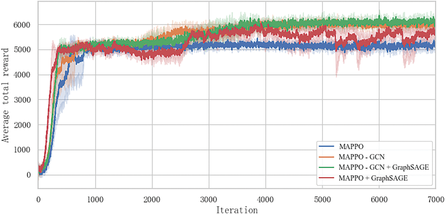
Figure 5: Comparison of average total rewards between MAPPO and its fusion of GCN and GraphSAGE variant algorithms during intelligent agent training

7  Conclusion

The experiment comprehensively verified the effectiveness of the GNN framework integrating GCN and GraphSAGE in multi-agent joint radar communication (JRC) systems. Through dynamic graph sampling and attention mechanisms, the new algorithm demonstrated superior performance to traditional methods in terms of communication success rate, decision speed, and environmental adaptability. The ablation experiments further clarified the roles of each module in the algorithm, providing direction for algorithm optimization and improvement. The hierarchical fusion path of GNN and DRL proposed in this study provides a more robust and deployable solution for real-time resource scheduling in vehicle-to-everything (V2X) and intelligent transportation systems, and is expected to have significant application value in high-density vehicle scenarios. In the future, we can further expand to complex traffic scenarios such as multi-lane roads and intersections, explore lightweight GNN architectures to reduce computational overhead, and integrate multi-sensor data to improve decision-making accuracy.

Acknowledgement: Not applicable.

Funding Statement: This research was funded by Shandong Provincial Natural Science Foundation, grant number ZR2023MF111.

Author Contributions: The authors confirm contribution to the paper as follows: Conceptualization, methodology and writing, Zeyu Chen; supervision and project administration, Jian Sun; formal analysis, Zhengda Huan; experimental verification, Ziyi Zhang. All authors reviewed the results and approved the final version of the manuscript.

Availability of Data and Materials: The authors confirm that the data supporting the findings of this study are available within the article.

Ethics Approval: Not applicable.

Conflicts of Interest: The authors declare no conflicts of interest to report regarding the present study.

Appendix A Derivation of the CLIP Loss Function

The CLIP loss function proposed in Section 4.2 of the main text is used to limit the policy update step size of MAPPO, preventing training oscillations caused by excessive parameter adjustments. Its core derivation process is as follows:

A.1 Definition of the Probability Ratio

In the MAPPO algorithm, the core basis for policy updates is the “ratio of the action probability of the current policy to that of the old policy” (probability ratio), defined as ρt(θk), πk(at|ot;θk) is the probability that agent k selects action at under the current policy parameter θk and observation ot; πk,old(at|ot;θk,old) is the old policy probability from the previous iteration (with fixed parameter θk,old), which is used to measure the relative magnitude of the policy update.

A.2 Construction Logic of the CLIP Loss Function

To avoid “abrupt policy changes” (e.g., a sudden shift from “prioritizing communication” to “prioritizing radar detection”) caused by excessively large or small ρt(θk), a clipping coefficient ε (set to ε=0.2 in the main text experiments) is introduced to constrain ρt(θk) within the interval [1−ε,1+ε], ensuring update stability.

The core idea of the CLIP loss function at this point is to “take the minimum of the ‘original probability ratio-weighted advantage’ and the ‘clipped probability ratio-weighted advantage’”. This not only uses the advantage function to guide policy optimization but also avoids over-updates through clipping (Eq. (13)).

Where τ∼πk,old denotes trajectories (including sequences of observations, actions, and rewards) sampled from the old policy, ensuring the unbiasedness of the expectation calculation; Atπk is the advantage function (Eq. (14) in the main text), which quantifies the value advantage of action at relative to the “average policy” (e.g., actions with high SINR and low AoI correspond to positive advantages, and vice versa for negative advantages); clip(⋅) is the clipping function: if ρt(θk)>1+ε, it takes 1+ε; if ρt(θk)<1−ε, it takes 1−ε; otherwise, the original value is retained.

References

1. Luong NC, Lu X, Hoang DT, Niyato D, Wang P, Kim DI. Radio resource management in joint radar and communication: a comprehensive survey. IEEE Commun Surv Tutor. 2021;23(2):780–814. doi:10.1109/COMST.2021.3057770. [Google Scholar] [CrossRef]

2. Hult R, Sancar FE, Jalalmaab M, Falcone P, Wymeersch H. Design and experimental validation of a cooperative driving control architecture for the grand cooperative driving challenge 2016. IEEE Trans Intell Transp Syst. 2018;19(4):1290–301. doi:10.1109/TITS.2017.2749978. [Google Scholar] [CrossRef]

3. Liu F, Masouros C, Petropulu AP, Griffiths H, Hanzo L. Joint radar and communication design: applications, state-of-the-art, and the road ahead. IEEE Trans Commun. 2020;68(6):3834–62. doi:10.1109/TCOMM.2020.2973976. [Google Scholar] [CrossRef]

4. Ma D, Shlezinger N, Huang T, Liu Y, Eldar YC. Joint radar-communication strategies for autonomous vehicles: combining two key automotive technologies. IEEE Signal Process Mag. 2020;37(4):85–97. doi:10.1109/MSP.2020.2983832. [Google Scholar] [CrossRef]

5. Kaul S, Gruteser M, Rai V, Kenney J. Minimizing age of information in vehicular networks. In: Proceedings of the 2011 8th Annual IEEE Communications Society Conference on Sensor, Mesh and Ad Hoc Communications and Networks; 2011 Jun 27–30; Salt Lake City, UT, USA. Piscataway, NJ, USA: IEEE; 2011. p. 350–8. doi:10.1109/SAHCN.2011.5984926. [Google Scholar] [CrossRef]

6. Ren P, Munari A, Petrova M. Performance analysis of a time-sharing joint radar-communications network. In: Proceedings of the 2020 International Conference on Computing, Networking and Communications (ICNC); 2020 Feb 17–20; Big Island, HI, USA. Piscataway, NJ, USA: IEEE; 2020. p. 908–13. doi:10.1109/ICNC47757.2020.9049747. [Google Scholar] [CrossRef]

7. Hsu YP, Modiano E, Duan L. Scheduling algorithms for minimizing age of information in wireless broadcast networks with random arrivals. IEEE Trans Mob Comput. 2019;19(12):2903–15. doi:10.1109/TMC.2019.2933780. [Google Scholar] [CrossRef]

8. Huang L, Modiano E. Optimizing age-of-information in a multi-class queueing system. In: Proceedings of the 2015 IEEE International Symposium on Information Theory (ISIT); 2015 Jun 14–19; Hong Kong, China. Piscataway, NJ, USA: IEEE; 2015. p. 1681–5. doi:10.1109/ISIT.2015.7282772. [Google Scholar] [CrossRef]

9. Talak R, Karaman S, Modiano E. Optimizing information freshness in wireless networks under general interference constraints. In: Proceedings of the Eighteenth ACM International Symposium on Mobile Ad Hoc Networking and Computing; 2018 Jun 26–29; Los Angeles, CA, USA. New York, NY, USA: ACM; 2018. p. 61–70. doi:10.1145/3209582.3209597. [Google Scholar] [CrossRef]

10. Chen ML, Ke F, Lin Y, Qin MJ, Zhang XY, Ng DWK. Joint communications, sensing, and MEC for AoI-aware V2I networks. IEEE Trans Commun. 2024;73(7):5357–74. doi:10.1109/TCOMM.2024.3401501. [Google Scholar] [CrossRef]

11. Sukhbaatar S, Fergus R. Learning multiagent communication with backpropagation. Adv Neural Inf Process Syst. 2016;29:1–9. [Google Scholar]

12. Singh A, Jain T, Sukhbaatar S. Learning when to communicate at scale in multiagent cooperative and competitive tasks. arXiv:1812.09755. 2018. [Google Scholar]

13. Samir M, Assi C, Sharafeddine S, Ebrahimi D, Ghrayeb A. Age of information aware trajectory planning of UAVs in intelligent transportation systems: a deep learning approach. IEEE Trans Veh Technol. 2020;69(11):12382–95. doi:10.1109/TVT.2020.3023180. [Google Scholar] [CrossRef]

14. Lorberbom G, Maddison CJ, Heess N, Hazan T, Tarlow D. Direct policy gradients: direct optimization of policies in discrete action spaces. Adv Neural Inf Process Syst. 2020;33:18076–86. [Google Scholar]

15. Mao H, Zhang Z, Xiao Z, Gong Z. Modelling the dynamic joint policy of teammates with attention multi-agent DDPG. arXiv:1811.07029. 2018. [Google Scholar]

16. Kopic A, Perenda E, Gacanin H. A collaborative multi-agent deep reinforcement learning-based wireless power allocation with centralized training and decentralized execution. IEEE Trans Commun. 2024;72(11):7006–16. doi:10.1109/TCOMM.2024.3401502. [Google Scholar] [CrossRef]

17. Xu L, Sun S, Zhang YD, Petropulu AP. Reconfigurable beamforming for automotive radar sensing and communication: a deep reinforcement learning approach. IEEE J Sel Areas Sens. 2024;1:124–38. doi:10.1109/JSAS.2024.3384567. [Google Scholar] [CrossRef]

18. Zhang Z, Wu Q, Fan P, Cheng N, Chen W, Letaief KB. DRL-based optimization for AoI and energy consumption in C-V2X enabled IoV. IEEE Trans Green Commun Netw. 2025;9(1):C2. doi:10.1109/TGCN.2025.3531902. [Google Scholar] [CrossRef]

19. Kipf TN, Welling M. Semi-supervised classification with graph convolutional networks. arXiv:1609.02907. 2016. [Google Scholar]

20. Hamilton WL, Ying Z, Leskovec J. Inductive representation learning on large graphs. Adv Neural Inf Process Syst. 2017;30:1–11. [Google Scholar]

21. Hieu NQ, Hoang DT, Niyato D, Wang P, Kim DI. Transferable deep reinforcement learning framework for autonomous vehicles with joint radar-data communications. IEEE Trans Commun. 2022;70(8):5164–80. doi:10.1109/TCOMM.2022.3183001. [Google Scholar] [CrossRef]

22. Sohaib RM, Onireti O, Sambo Y, Swash R, Imran M. Energy efficient resource allocation framework based on dynamic meta-transfer learning for V2X communications. IEEE Trans Netw Serv Manag. 2024;21(4):4343–56. doi:10.1109/tnsm.2024.3400605. [Google Scholar] [CrossRef]

23. Zheng B, Liang H, Ling J, Gong S, Gu B. Integrating graph neural networks with multi-agent deep reinforcement learning for dynamic V2X communication. In: Proceedings of the 2024 20th International Conference on Mobility, Sensing and Networking (MSN); 2024 Dec 20–22; Harbin, China. Piscataway, NJ, USA: IEEE; 2024. p. 398–405. doi:10.1109/MSN60784.2024.00105. [Google Scholar] [CrossRef]

24. Fan Y, Fei Z, Huang J, Xiao Y, Leung VCM. Reinforcement learning-based resource allocation for multiple vehicles with communication-assisted sensing mechanism. Electronics. 2024;13(13):2442. doi:10.3390/electronics13132442. [Google Scholar] [CrossRef]

25. Zeng Y, Liu Q, Dai T, Huang Y, Hou R, Gan Y, et al. Resource optimization-oriented method for generating cooperative interference strategies. In: Proceedings of the 2023 International Conference on Intelligent Communication and Computer Engineering (ICICCE); 2023 Nov 24–26; Changsha, China. Piscataway, NJ, USA: IEEE; 2023. p. 37–46. doi:10.1109/ICICCE60048.2023.00015. [Google Scholar] [CrossRef]

26. Zhu J, He H, He Y, Fang F, Huang W, Zhang Z. Joint optimization of user scheduling, rate allocation, and beamforming for RSMA finite blocklength transmission. IEEE Internet Things J. 2024;11(10):17932–45. doi:10.1109/JIOT.2024.3366449. [Google Scholar] [CrossRef]

27. Ji M, Wu Q, Fan P, Cheng N, Chen W, Wang J, et al. Graph neural networks and deep reinforcement learning based resource allocation for V2X communications. IEEE Internet Things J. 2024;11(5):7892–905. doi:10.1109/JIOT.2023.3321521. [Google Scholar] [CrossRef]

28. Liu X, Zhang H, Long K, Nallanathan A. Proximal policy optimization-based transmit beamforming and phase-shift design in an IRS-aided ISAC system for the THz band. IEEE J Sel Areas Commun. 2022;40(7):2056–69. doi:10.1109/JSAC.2022.3155508. [Google Scholar] [CrossRef]

29. Schulman J, Wolski F, Dhariwal P, Radford A, Klimov O. Proximal policy optimization algorithms. arXiv:1707.06347. 2017. [Google Scholar]