
 Submit a Paper
 Propose a Special lssue
 Open Access
ARTICLE

Zero-Shot Vision-Based Robust 3D Map Reconstruction and Obstacle Detection in Geometry-Deficient Room-Scale Environments
Computer Science Department, Kyonggi University, Suwon, 16227, Republic of Korea
* Corresponding Author: Junho Ahn. Email:
Computers, Materials & Continua 2026, 86(2), 1-30. https://doi.org/10.32604/cmc.2025.071597
Received 08 August 2025; Accepted 23 October 2025; Issue published 09 December 2025
 View Full Text
 Download PDF
Abstract
As large, room-scale environments become increasingly common, their spatial complexity increases due to variable, unstructured elements. Consequently, demand for room-scale service robots is surging, yet most technologies remain corridor-centric, and autonomous navigation in expansive rooms becomes unstable even around static obstacles. Existing approaches face several structural limitations. These include the labor-intensive requirement for large-scale object annotation and continual retraining, as well as the vulnerability of vanishing point or line-based methods when geometric cues are insufficient. In addition, the high cost of LiDAR and 3D perception errors caused by limited wall cues and dense interior clutter further limit their effectiveness. To address these challenges, we propose a zero-shot vision-based algorithm for robust 3D map reconstruction in geometry-deficient room-scale environments. The algorithm operates in three layers: Layer 1 performs dimension-wise boundary detection; Layer 2 estimates vanishing points, refines the precise perspective space, and extracts a floor mask; and Layer 3 conducts 3D spatial mapping and obstacle recognition. The proposed method was experimentally validated across various geometric-deficient room-scale environments, including lobbies, seminar rooms, conference rooms, cafeterias, and museums—demonstrating its ability to reliably reconstruct 3D maps and accurately recognize obstacles. Experimental results show that the proposed algorithm achieved an F1 score of 0.959 in precision perspective space detection and 0.965 in floor mask extraction. For obstacle recognition and classification, it obtained F1 scores of 0.980 in obstacle absent areas, 0.913 in solid obstacle environments, and 0.939 in skeleton-type sparse obstacle environments, confirming its high precision and reliability in geometric-deficient room-scale environments.Keywords
Evolving lifestyles now keep individuals inside room-scale environments for progressively longer periods devoted to living, leisure, and work. In response, the architectural community is rapidly adopting large, room-scale indoor spaces—such as open lobbies, expansive lounges, and shared offices—that provide long, unobstructed sight lines. Because these spacious interiors are continually reconfigured with movable furniture, mobile partitions, and sculptural installations, their spatial complexity and irregularity increase rapidly. Driven by growing demand for room-scale services—such as cleaning, security, and item delivery, the global indoor service-robot market is projected to expand from USD 14.6 billion in 2025 to USD 30.5 billion by 2030 [1]. Yet because of technical constraints, most commercial delivery and security robots remain confined to corridor-centric operation. Although active research is pushing beyond corridor navigation toward fully autonomous motion inside large rooms, the ICRA 2024 BARN Challenge reported that robots still could not reliably traverse static-obstacle courses [2].
Existing attempts to overcome robots’ limited accessibility in room-scale environments fall into three categories, each with notable drawbacks. First, several studies construct large, labeled datasets and repeatedly retrain object models to cope with indoor, room-scale scenes. However, the rise of remote work and the growing demand for healthier indoor conditions, e.g., improved air quality—have spawned a wide variety of products, personalized decorative elements, and movable furnishings. This diversification has markedly increased the complexity of room-scale environments, so training on every object through exhaustive supervised learning now entails prohibitive time and cost. Second, several studies perform 3D scene understanding and object localization in room-scale environments by detecting geometric features and analyzing vanishing points [3]. However, methods that rely on perspective line and vanishing point detection are highly vulnerable to irregular interior layouts and complex furniture arrangements, which leads to a substantial drop in accuracy. The problem becomes even more challenging in large rooms, where reference geometric cues—such as side walls—are often insufficient or ambiguous, and the abundance of diverse furnishings and decorative installations further limits the applicability of traditional geometry-based detection. Third, some studies attempt to enhance camera-based depth estimation by incorporating expensive LiDAR sensors [4]. Although integrating high-resolution LiDAR can improve the accuracy of existing vision-based 3D perception algorithms, the additional hardware cost is prohibitive. According to a 2025 market survey [5], commercial LiDAR modules range in price from USD 500 to 75,000, depending on performance and application. In contrast, camera modules are significantly more affordable, typically ranging from USD 20 to 500.
The main technical challenge lies in the inability of monocular depth-estimation methods to reconstruct a globally consistent perspective frame in large, complex room-scale environments, despite their effectiveness in inferring pixel-level depth values from single RGB images [6]. However, they fall short of recovering a globally consistent perspective frame in generic room-scale environments—exactly the capability targeted in this study. Existing zero-shot, general-purpose 3D mapping algorithms attempt to infer the perspective frame from wall pixels, which provide strong geometric cues. In large room-scale environments, however, wall observations are often sparse or occluded by clutter, resulting in frequent errors in 3D scene understanding and hindering robust object-shape extraction.
To overcome these limitations, we propose a zero-shot general-purpose AI based, three-layer robust 3D map reconstruction algorithm. The method does not rely on corridor-centric geometric priors. It reconstructs missing dimensional spatial cues and accurately restores the 3D layout in room-scale interiors where complex furnishings and decorative elements are intermixed. In addition, the proposed algorithm recognizes and classifies both solid obstacles (e.g., boxes, trash bins) and sparse, skeleton-type obstacles (e.g., chairs, desks), which are typically challenging for depth estimation and mask extraction. It also estimates a floor mask and a precision perspective space, producing core inputs for 3D mapping. By fusing these components, the approach achieves high-quality 3D reconstruction cost-effectively, without resorting to high-cost sensors. Moreover, because the proposed method performs frame-wise three-layer robust 3D map reconstruction, it extracts frame-specific geometric cues even when dynamic obstacles are present within the field of view. Consequently, the substantial frame-to-frame variations introduced by dynamic obstacles are explicitly integrated into the spatial representation, enabling per-frame 3D spatial mapping and obstacle recognition. The differentiating features are summarized in three points. First, without large-scale labeling and retraining for all object categories, we fuse the pre-trained representations of a foundation model with a vision algorithm to secure a zero-shot general-purpose spatial inference capability that can be applied immediately even in new room-scale environments. Second, the proposed algorithm hierarchically fuses floor masks, vanishing point detection data, and perspective space data. Through this fusion, the proposed algorithm remains effective even when geometric cues—such as continuous walls or regularly aligned structures—are sparse or absent in large, complex room-scale environments. It reconstructs insufficient dimensional spatial data and achieves accurate recognition and classification of 3D space and obstacles. Third, by operating with only a single low-cost camera input, we implement a cost-effective vision system that acquires precise dimensional spatial data without expensive sensors such as LiDAR.
Indoor object detection suffers performance degradation due to background noise, occlusions, and multi-scale variation, and RGBD–centric datasets lack diversity in scenes, viewpoints, and classes for 2D detection research. To address this, Indoor-COCO was built by selecting challenging indoor images from COCO—11,302 images across eight classes [7]. Using this dataset, DINO [8] and its indoor-specialized extension I-DINO [9] were proposed. The DINO-based indoor detector was further strengthened with four modules, yielding improved performance. However, from a practical standpoint, adding Res2Net101 and GBi-FPN increases computational and memory requirements, hindering deployment on low-cost, CPU-based robots. In addition, the training stability of Deformable Attention can be sensitive to hyperparameters and data quality, so convergence may slow under rapidly changing illumination or high sensor noise. In addition, SIoU Loss can amplify errors when label boxes are inaccurate; consequently, localization deviations may increase for tiny objects such as wires and plants, revealing a limitation.
In another study, the floor was identified using a learning-based segmentation method, after which a lightweight, geometry-based tracking strategy analyzed floor patterns to detect obstacles, estimate distances, and build a real-time map in the cloud [10]. However, this approach is prone to false positives under lighting changes and shadows; its distance estimation relies on simple odometry, yielding low precision; the experiments were restricted to straight corridors, making generalization to complex spaces difficult; and the Region-of-Interest (ROI) bounds limit the detection of small or distant obstacles.
Foundation models, pre-trained on large-scale multimodal data, emphasize zero-shot capability: enabled by their general-purpose representations, they can perform inference immediately on tasks and domains for which they were not explicitly trained. From the perspective of visual understanding, CLIP [11] established the standard for zero-shot recognition by contrastively learning from web image-text pairs and classifying unseen classes using only text prompts, while SimCLR [12] demonstrated the potential of a self-supervised backbone that learns from unlabeled images via augmentation and contrastive loss and solves downstream tasks with little to no fine-tuning. On the generative side, Stable Diffusion [13] combined language conditioning with a diffusion process compressed with VQ-VAE [14], thereby popularizing zero-shot text-to-image synthesis on GPUs for consumer use. In the multimodal LLM line, DeepMind’s Flamingo [15] placed visual attention layers on top of a large language model to perform image-to-text questions answering with only few-shot in-context examples. The research trajectory has progressed from task-specialized models to unified vision models, then to multimodal large language models, and ultimately to multimodal agents that invoke multiple tools to accomplish tasks [16]. Along this path, foundation models have continually advanced zero-shot generalization, indicating an expansion from domain-expert performance to general vision-language assistants. This developmental history provides key prior context for the goal of this paper—zero-shot robot intelligence for indoor spatial perception, which interprets complex, unstructured environments without additional fine-tuning. In another line of work, the zero-shot knowledge of foundation vision-language models were leveraged to immediately interpret complex indoor spaces (e.g., shopping malls and underground areas) from a single RGB camera and to build a 3-D map [17]. By merging floor masks and fusing variable vanishing points, the method achieved F1 scores of 0.965 for floor detection and 0.93 for obstacle detection; however, performance degraded under abrupt illumination changes, complex floor patterns, and overlapping ROI, and limits were observed in fine-grained class classification.
Depth estimation is central to 3D scene understanding. Approaches fall broadly into two groups: active sensing using LiDAR, ToF, or structured light, and passive (monocular) methods that reconstruct depth from a single RGB image. A recent review [18] divides monocular depth estimation into three periods. In the first period, traditional methods dominated, leveraging diverse geometric/photometric cues such as structured light, contours, texture, shading, multifocus, and SfM. In the second period, parametric or non-parametric regression models based on MRF and CRF emerged, spreading machine learning approaches. The third period began with the introduction of deep learning—starting from early pure CNNs, moving to CNN–CRF hybrids, then expanding to RNNs and ConvLSTM [19], and most recently evolving toward Transformers [20] and their integration with vision transformers. Recent deep models are trained on large-scale RGBD benchmarks such as NYU-Depth v2 [21], KITTI [22], and Cityscapes [23], and are evaluated with standard metrics including RMS, ABS Rel, and δ < 1.25. Beyond supervised learning, semi-supervised and self-supervised techniques directly regress absolute depth. In parallel, strategies such as multi-scale encoder-decoder designs, self-attention, cost-volume regularization, and image-radar fusion are used to capture global context and local geometry simultaneously. Nevertheless, several challenges persist. These include sensitivity to illumination changes, transparent and reflective materials, and dynamic occlusions, along with limited ground-truth for absolute depth and inherent scale ambiguity. Another study, Depth-Pro [24] reconstructs the research landscape of monocular depth estimation as a fine-grained hierarchical roadmap. It categorizes progress into seven streams: traditional geometric/photometric methods; MRF-based machine learning; CRF-based machine learning; CNNs; Transformers [20]; GAN-based [25]; and VAE-based [26] deep learning. Representative methods—such as Swin Transformer [27], AdaBins [28], and BinsFormer [29]—are compared on common datasets and metrics, and trade-offs are analyzed on NYU-Depth v2 [21], KITTI [22], and others. While Transformers achieve high accuracy by capturing global context, they remain limited by demands for large-scale data and substantial computational resources.
Vanishing point detection is often used to infer orientation immediately in indoor scenes with many parallel structures, such as corridors. One approach [3] first extracts the wall-floor and wall-ceiling boundary lines using line-segment extraction and clustering. From pairwise intersections of these boundary pairs, it then forms up to six vanishing-point hypotheses. A fast consistency check selects the dominant vanishing point by iteratively minimizing the dispersion among hypothesis distances and correcting/pruning low-consistency boundaries. However, when vertical boundaries are scarce or the robot is close to a side wall, vanishing point candidates become overly dispersed, leading to boundary false positives or missed detections. Moreover, when the ceiling region occupies only a small portion of the frame, the ceiling hypothesis is invalidated, and the global structural estimate becomes unstable. Consequently, the technique is specialized for straight corridors with sufficient boundary lines, and it shows limitations in open lobbies or non-rectilinear, unstructured spaces. Table 1 summarizes the main methods, evaluation datasets, and performance results reviewed in Section 2.

This study proposes a zero-shot, vision-based, three-layer algorithm for robust 3D map reconstruction. In large, complex room-scale environments, the method hierarchically fuses detected floor mask and precision perspective spaces to reconstruct missing dimensional spatial data. It also recognizes and classifies both solid obstacles and sparse, skeleton-type obstacles. Fig. 1 illustrates the overall architecture and processing workflow of the proposed algorithm.
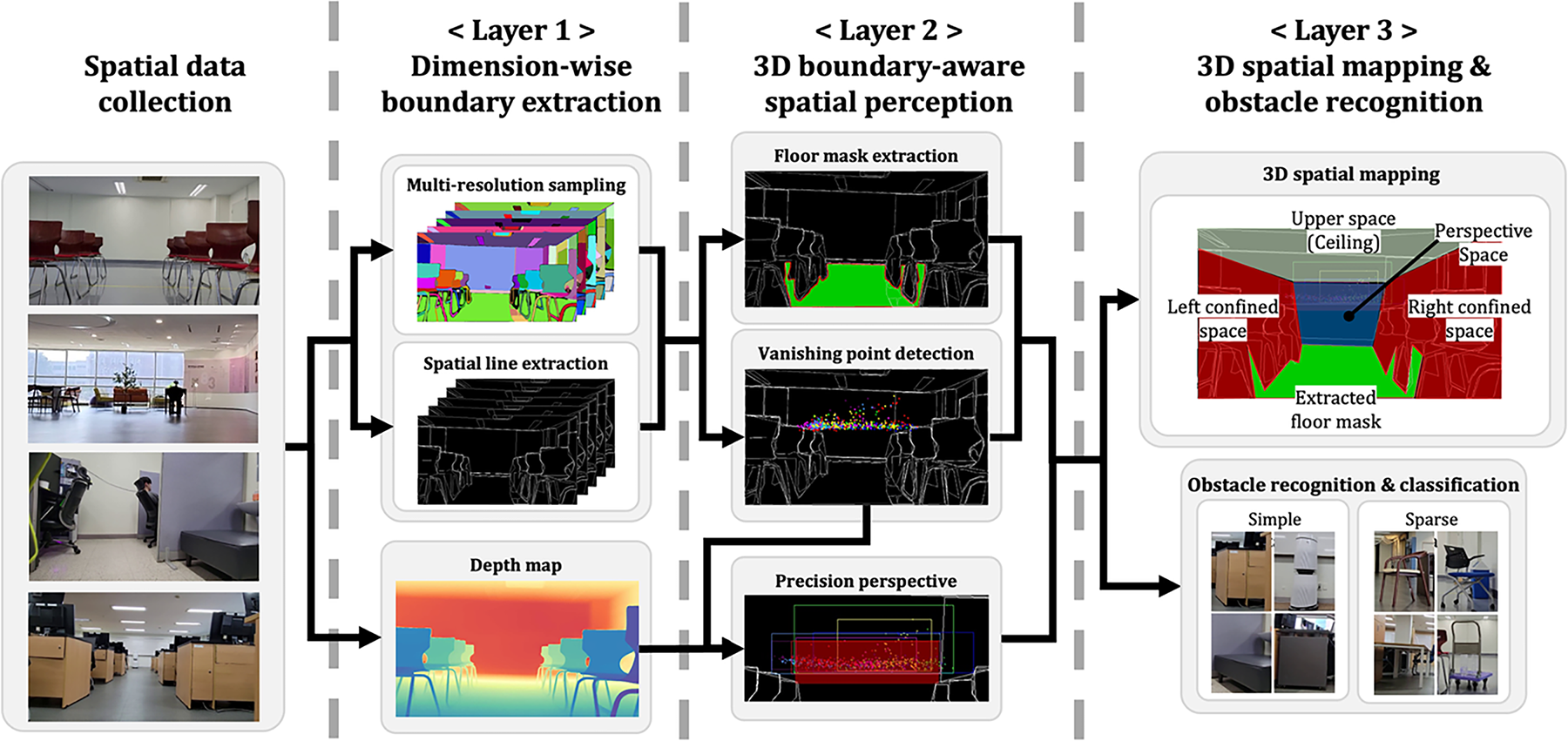
Figure 1: Processing pipeline of the proposed algorithm
The proposed three-layer robust 3D map reconstruction algorithm takes as input RGB frames captured by a single camera in geometry-deficient room-scale environments where only one wall—or virtually no visible walls—is present. It generates 3D spatial-mapping data in settings where solid and sparse, skeleton-type obstacles—e.g., interior objects, cleaning tools, office supplies, chairs, and desks—are intermixed. The algorithm comprises three layers. Layer 1 (Dimension-wise boundary extraction) quantitatively estimates the minimum and maximum extents along the x, y, and z axes from the input 2-D image and numerically characterizes the outer boundary of the space. It then detects boundary lines for each dimension. Layer 2 (3D boundary-aware spatial perception) uses the dimension-wise boundaries from layer 1 to detect vanishing points, then performs refined perspective frame estimation based on the vanishing-point data. It also obtains a clean floor mask—separated from obstacles—using segmentation masks. Thus, the system provides a structural representation of the space instead of a set of numeric bounds. Layer 3 (3D spatial mapping & obstacle recognition) fuses the dimension-wise boundaries, floor mask, and refined perspective frame to construct the 3D spatial map. Using the fused data, it recognizes obstacles in the scene and performs fine-grained obstacle classification, explicitly identifying skeleton-structured sparse obstacles. Fig. 2 details workflow of the proposed three-layer robust 3D map reconstruction algorithm.
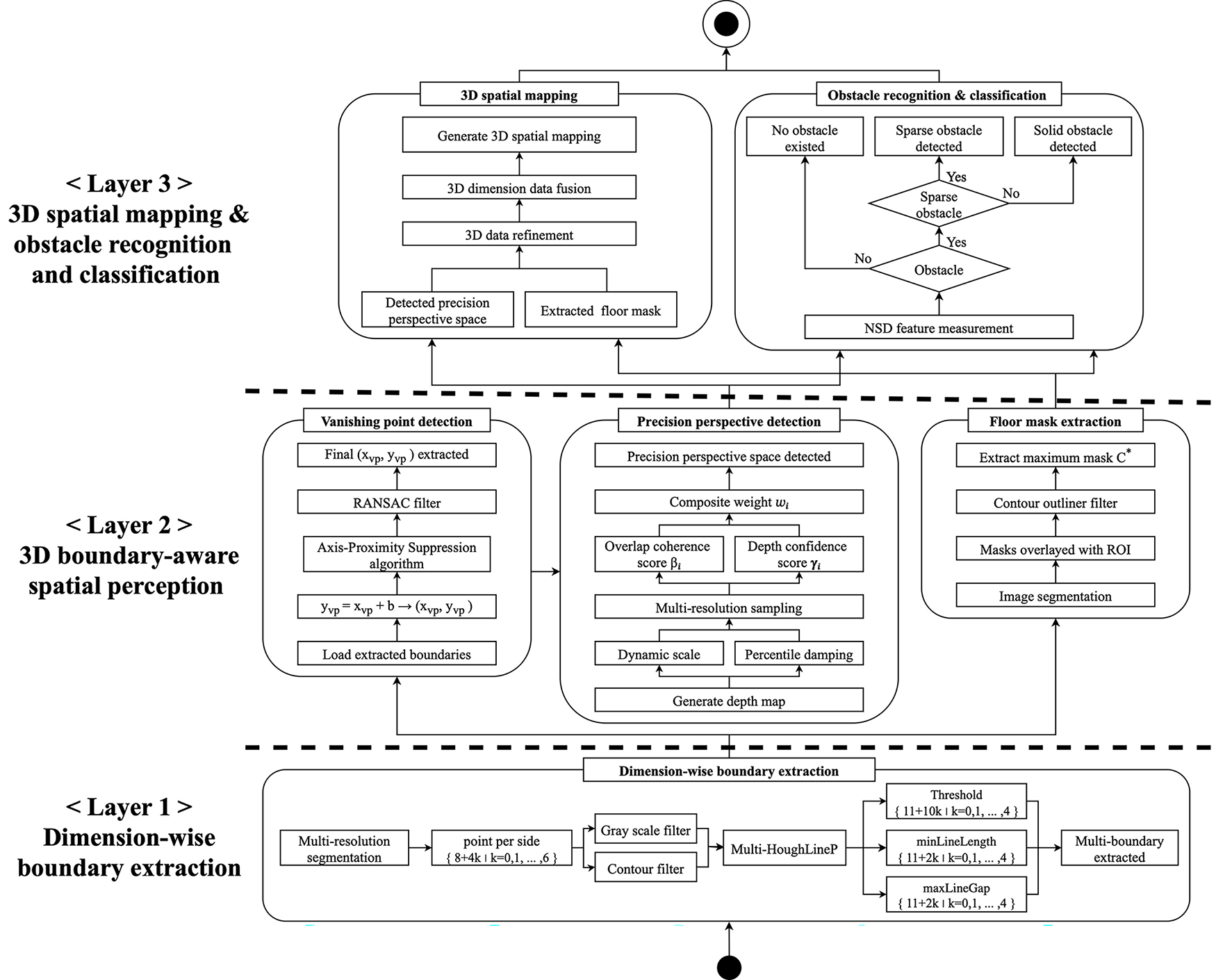
Figure 2: Three-layer robust 3D map reconstruction algorithm
3.2 Limitations of Prior Research
Large indoor venues, such as shopping malls and underground spaces, exhibit complex patterns and frequent layout changes. In such settings, it is difficult to rely on expensive LiDAR or on models that must be retrained for each environment. To address this, our prior research proposed a zero-shot general-purpose 3D mapping algorithm that immediately interprets complex scenes and builds up-to-date 3D maps [17]. An initial floor mask obtained from a foundation model is merged using ROI and depth-similarity criteria to convert complex textures into a single, continuous corridor region. The method then fuses edge-based and depth-based vanishing points with a dynamically weighted pyramid scheme, securing stable orientation across diverse layouts. For obstacle detection, three modules, respectively exploit the floor–vanishing-point distance, the dispersion of vanishing-point coordinates, and the depth distribution. Consequently, high-precision identification is achieved even for sparse obstacles with large voids (e.g., lattice steel racks). Tests on low-cost robots with a monocular RGB camera achieved F1 scores of 0.965 for floor detection and 0.93 for obstacle detection, outperforming recent foundation segmentation models such as Segment Anything Model 1 (SAM1) [30], Segment Anything Model 2 (SAM2) [31], and Simple Click [32].
Our prior research operates relatively robustly in straight-corridor settings because they rely heavily on floor-mask patterns and side walls. However, in large, geometry-deficient, room-scale environments where geometric cues are insufficient, single vanishing point detection becomes inaccurate and floor-wall boundaries grow ambiguous, degrading the accuracy of 3D scene understanding. Accordingly, to address these limitations, this research suggests a three-layered robust 3D map reconstruction algorithm that reconstructs dimension-wise spatial boundaries in large, complex room-scale environments with insufficient geometric information. The proposed method generates 3D spatial mapping data by leveraging floor masks and precision perspective regions, while simultaneously enabling recognition and classification of both solid obstacles and skeleton-type sparse obstacles. Compared with prior research, the proposed algorithm presents the following technical improvements. First, it enables zero-shot 3D spatial mapping as well as obstacle recognition and classification in geometry-deficient, large, complex room-scale environments. This capability overcomes the limitations of prior research, which was restricted to linear corridor-like environments. Second, it reconstructs dimension-wise boundaries even in geometry-deficient environments, generating precision perspective regions through multiple vanishing points. This approach addresses the inaccuracy of the single-vanishing-point method employed in prior work. Third, through layer 2’s 3D boundary-aware spatial perception, it extracts accurate floor masks even when sparse obstacles are present and floor-wall boundaries are ambiguous. This resolves the boundary ambiguity issue observed in prior research.
3.3 Definition and Data Analysis
In this study, we define ‘large, complex room-scale environments as consisting of two types. First, lobby-type spaces in which one or fewer walls are visible, yielding open lines of sight and weak directional cues. Second, composite spaces—such as offices or cafés—where solid obstacles and sparse obstacles are intermingled. Here, a solid obstacle denotes an object with a fully enclosed volume that is completely separated from the surroundings (e.g., boxes, trash bins), whereas a sparse obstacle refers to an object with a skeleton-like structure, a partially open frame whose interior is visible (e.g., chairs, desks), i.e., an object whose volume is not fully sealed.
To derive spatial patterns that generalize to complex interiors, public datasets and indoor image data were analyzed [33]. The analysis indicates that the placement of indoor furniture and structures is not random; rather, it follows repeatable structural patterns grounded in human-factors design principles—such as circulation, visual balance, and spatial partitioning [34,35]. Obstacles were further divided into solid and sparse classes, and their visual and reflective characteristics were quantitatively compared. The results show that sparse obstacles exhibit structurally incomplete boundaries, low feature density, and reflective components, making them substantially harder for conventional vision algorithms to detect [36]. These observations support the need for a zero-shot approach capable of inferring spatial structure without supervised retraining. Fig. 3 summarizes representative examples of solid obstacles, sparse obstacles, and the large, complex room-scale environments defined in this work.
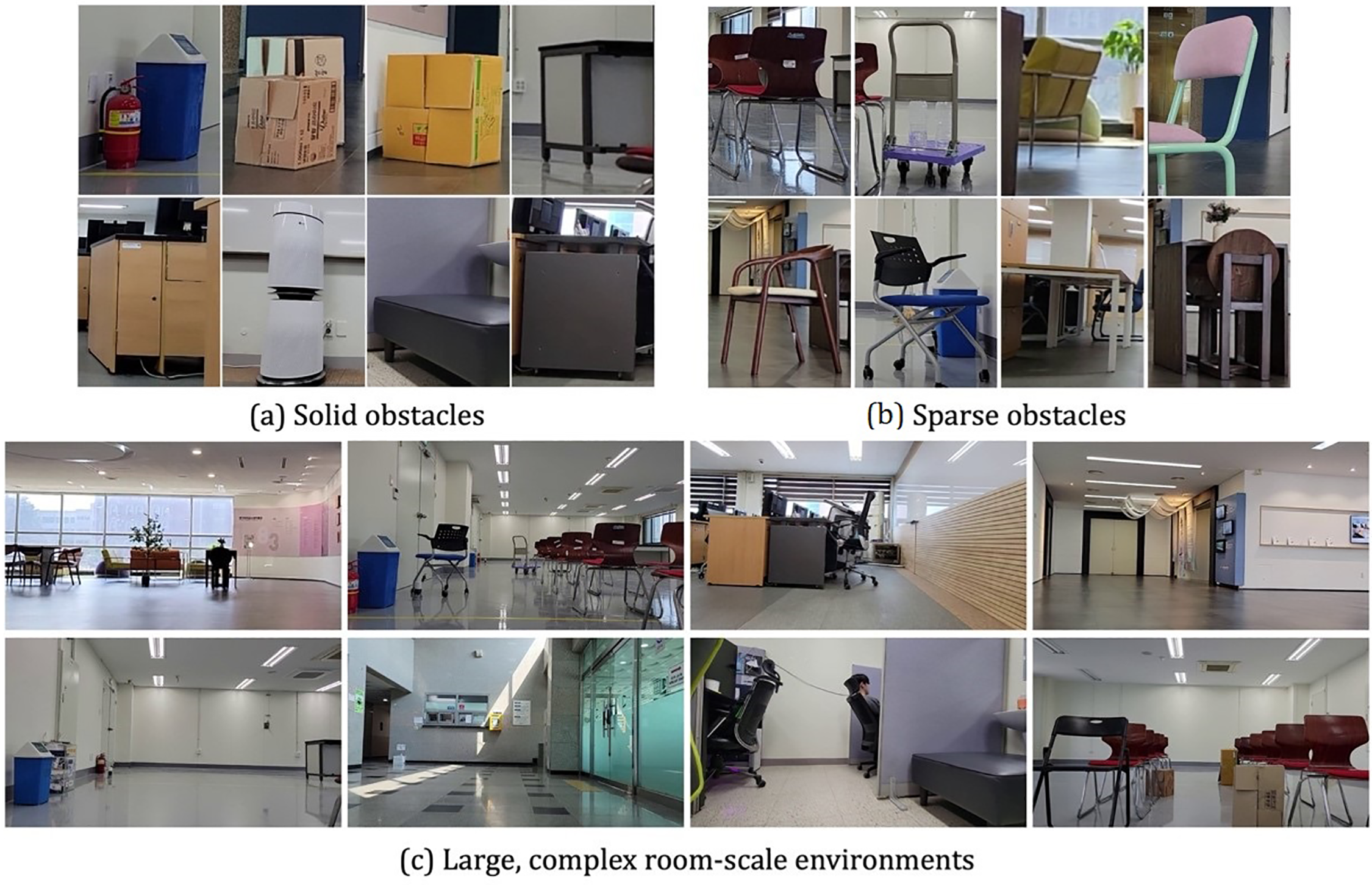
Figure 3: Example images defined in this study: (a) solid obstacles, (b) sparse obstacles, and (c) large, complex room-scale environments
3.4 Layer 1: Dimension-Wise Boundary Extraction
Layer 1 performs dimension-wise boundary extraction, quantifies the minimum and maximum spatial extents along the x, y, and z axes from the input 2D image. Based on these quantified ranges, it extracts axis-aligned boundary lines, effectively delineating the outer structure of the observed space. This process yields reliable dimensional constraints in room-scale indoor environments where walls are sparse or entirely absent, and obstacles are densely distributed. Such constraints are particularly critical in settings where perspective cues are insufficient. The extracted dimensional boundaries serve as essential priors for subsequent vanishing point detection and fine-grained perspective estimation. They contribute to reducing false detections, improving geometric consistency, and stabilizing scene scale. Moreover, these boundaries provide structural guidance for isolating accurate floor masks from segmentation outputs by excluding regions associated with detected objects. Additionally, background noise—including shadows, strong illumination, and light reflections—is suppressed through appropriate preprocessing in layer 1. During this stage, dimension-wise boundary extraction employs multi-resolution segmentation in combination with grayscale and contour filtering to preprocess noise from the input data. Consequently, the algorithm is able to extract geometric information robustly even under severe noise conditions, thereby enabling reliable spatial perception, integration, and the generation of accurate 3D spatial mapping data for obstacle recognition and classification.
To extract initial object masks, we utilize SAM1 with a multi-resolution sampling strategy instead of using a fixed value for its points per side (pps) parameter. Pps denotes the number of evenly spaced grid points per side of the input image; increasing it raises sampling density. For each image, we vary pps across seven levels: {8 + 4k | k = 0, 1, …, 6}, enabling dense sampling across multiple resolutions. The resulting global mask set
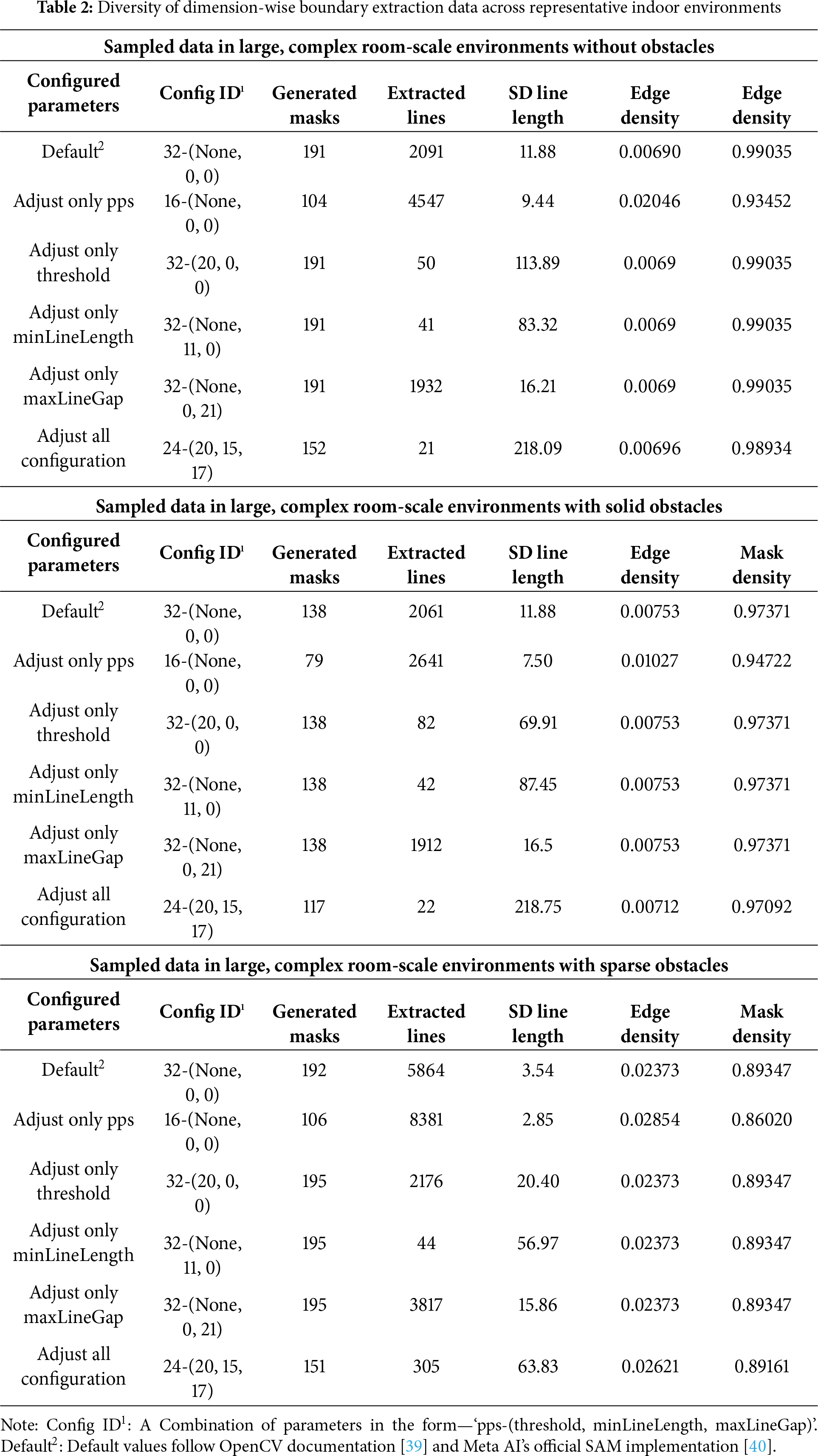
Table 2 categorizes large, complex room-scale environments into three types based on the presence and characteristics of obstacles. For each type, we analyze the key visual properties extracted using multi-resolution sampling and diverse parameter configurations for line detection. These results are compared against a baseline set using default parameter settings. The evaluated features include the number of masks, number of detected lines, standard deviation of line lengths, edge density, and mask density. These features are critical for vanishing point estimation, precision perspective detection, and floor mask extraction. By comparing across conditions, the table quantitatively demonstrates the variability and richness of visual features induced by parameter changes. This analysis highlights how parameter tuning affects spatial boundary extraction and the expressiveness of scene representation.
3.5 Layer 2: 3D Boundary-Aware Spatial Perception
3.5.1 Vanishing Point Detection
Based on the layer 1: dimension-wise boundary extraction results, this study derives robust multi-vanishing points
3.5.2 Precision Perspective Detection
To enable accurate perspective detection, a two-step process is designed. Step 1 maps the distribution of vanishing points—obtained from multi-resolution sampling—to a scale factor that implicitly encodes depth information. Two algorithms, percentile damping and dynamic scale weighting, are introduced and applied. These algorithms inject the scale factor into an exponential weighting function to nonlinearly amplify the reliability of vanishing points that contribute more significantly to depth inference. Through this approach, perspective regions are independently detected at each resolution level. Step 2 integrates the perspective region estimates derived from different resolutions. A composite weight is defined by combining two scores: the overlap coherence score, which is based on the intersection area between candidate regions, and the depth confidence score, which reflects the magnitude of depth. This weighting method selectively reinforces candidates that meet both spatial consistency and depth plausibility. The proposed strategy effectively mitigates vanishing point errors caused by nearby objects and robustly produces a single bounding box that defines the precision perspective space. Fig. 4 illustrates the proposed pipeline for precision perspective detection.
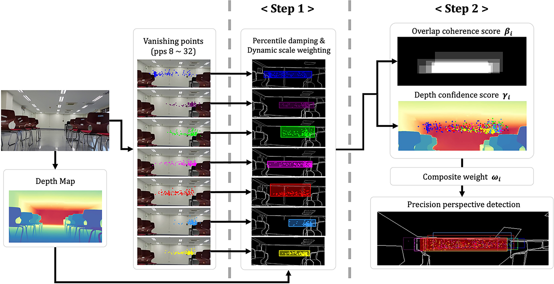
Figure 4: Detailed process of precision perspective detection
Step 1 begins by generating a depth map from each image of the room-scale environments dataset using Depth-Pro, which performs monocular depth estimation. The resulting depth map
Step 2 computes the weighted centroid
Based on the two independently computed metrics—overlap coherence score
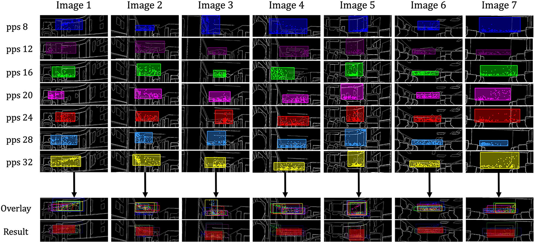
Figure 5: Multi-resolution fusion for precision perspective detection
The proposed process aims to achieve accurate floor mask extraction in large, complex room-scale environments with densely arranged obstacles, as depicted in Fig. 6. First, the input image is defined with dimensions
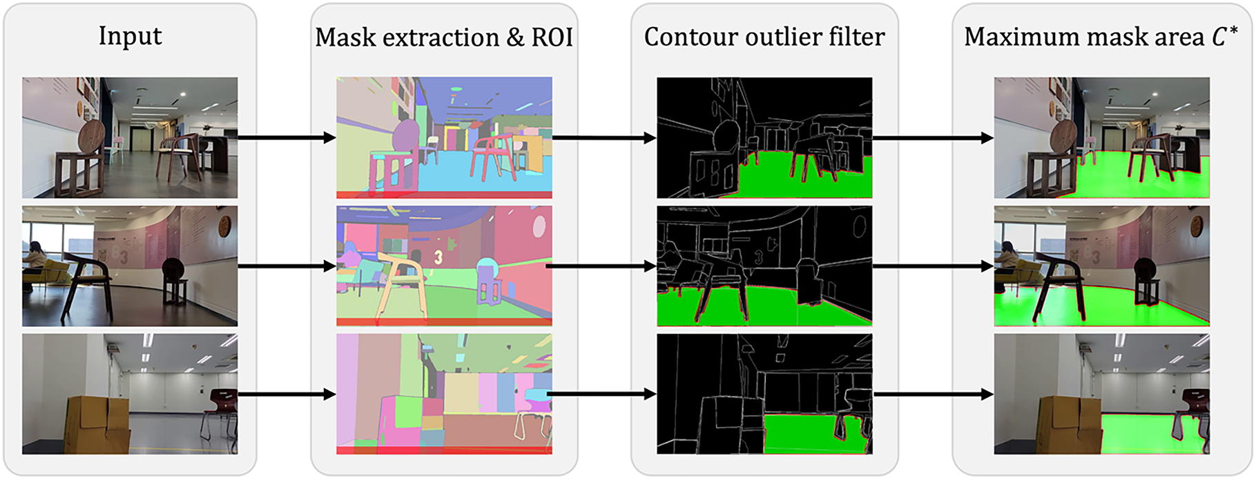
Figure 6: Detailed process of floor mask extraction
3.6 Layer 3: 3D Spatial Mapping & Obstacle Recognition
Through the fusion of layer 1 and layer 2, dimension-wise boundary data, vanishing points, precision perspective space, and floor mask information are obtained. These outputs are integrated to construct a 3D spatial mapping, as illustrated in Fig. 7. This 3D spatial mapping serves as the core representation for interpreting room-scale indoor images in three dimensions. It is particularly critical for robust 3D map reconstruction in geometry-deficient room-scale environments. The fused mapping defines the region from the precision perspective space down to the floor mask as a confined space, bounded laterally. The space directly above the perspective region is defined as upper space, typically corresponding to ceiling areas. This structured representation enables mobile robots to distinguish among four spatial categories: traversable floor regions, open forward spaces, laterally confined areas caused by obstacles or structural elements, and upper regions with minimal constraints. This approach enables the system to enhance environmental understanding in large, complex room-scale environments.
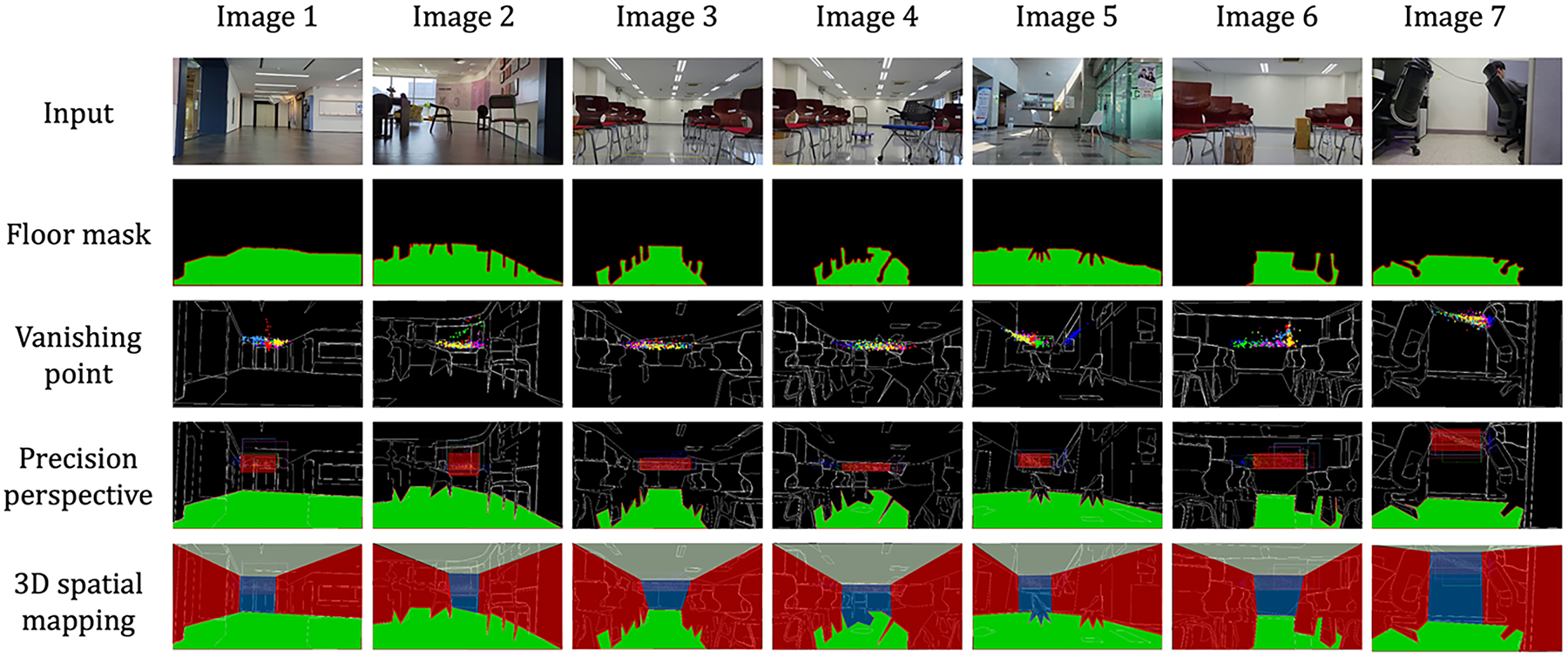
Figure 7: Constructed 3D spatial mapping in large, complex room-scale environments
3.6.2 Obstacle Recognition & Classification
In prior research on zero-shot general-purpose 3D mapping algorithms, obstacle detection was based on analyzing the variance of vanishing point coordinates across consecutive frames, which varied with obstacle type. However, dispersion of coordinates alone is insufficient for robust obstacle recognition and classification in geometry-deficient room-scale environments. To overcome this limitation, a Normalized Spatial Dispersion (NSD) metric is proposed to classify solid and sparse obstacles using precision perspective space and floor mask information. NSD converts pixel coordinates into a dimensionless normalized space and quantifies spatial spread to determine the presence of obstacles and differentiate between solid and sparse types.
As an initial step, the floor mask detected from large, complex room-scale environments is excluded from the target region for obstacle recognition and classification. This step eliminates unnecessary exploration and computation in advance. For each continuous frame
4.1 Experiments Setup and Data Collection
To validate the proposed algorithm, we conducted an ablation study on the vanishing point detection method used for precision perspective space detection and compared multi-resolution sampling with fixed-resolution sampling. We further performed comparative evaluations against prior research on precision perspective space detection and floor mask extraction. Finally, we compared the proposed method with existing approaches on obstacle recognition and classification between solid and sparse obstacles.
For the experiments, we captured and collected approximately 40,000 images of large, complex room-scale environments. As illustrated in Fig. 8, data acquisition employed an OMOROBOT R1 V2 robot [43] and a Samsung Galaxy S21+, with the smartphone mounted on the top of the robot while it traversed at 0.4 m/s. The experimental R1 V2 robot, equipped with a smartphone, navigated through a large, complex room-scale environment, capturing scenes within its field of view using the smartphone camera to collect data and conduct experiments. To ensure the reliability of validation through experiments with diverse forms and varying levels of complexity, this research selected geometry-deficient spaces from twelve distinct large, complex room-scale environments—including museum lobby, museum cafeteria, seminar room passageway, office room passageway, and conference room passageway—for data collection and experimental evaluation. The experimental settings also encompassed extreme scenarios, including indoor environments with strong illumination and light reflections as well as severe occlusions caused by obstacles, thereby ensuring validation of their diversity and complexity. Image data were gathered in three scenarios: (1) obstacle absent room-scale indoor environments; (2) environments with solid obstacles placed ahead; and (3) environments with sparse obstacles placed ahead. Experiments were conducted on high-performance hardware, including an Intel i9-13900K CPU with an NVIDIA GeForce RTX 4090 GPU, an Intel i9-10900K with an RTX 4080, and an Intel i7-10700 with an RTX 3090.
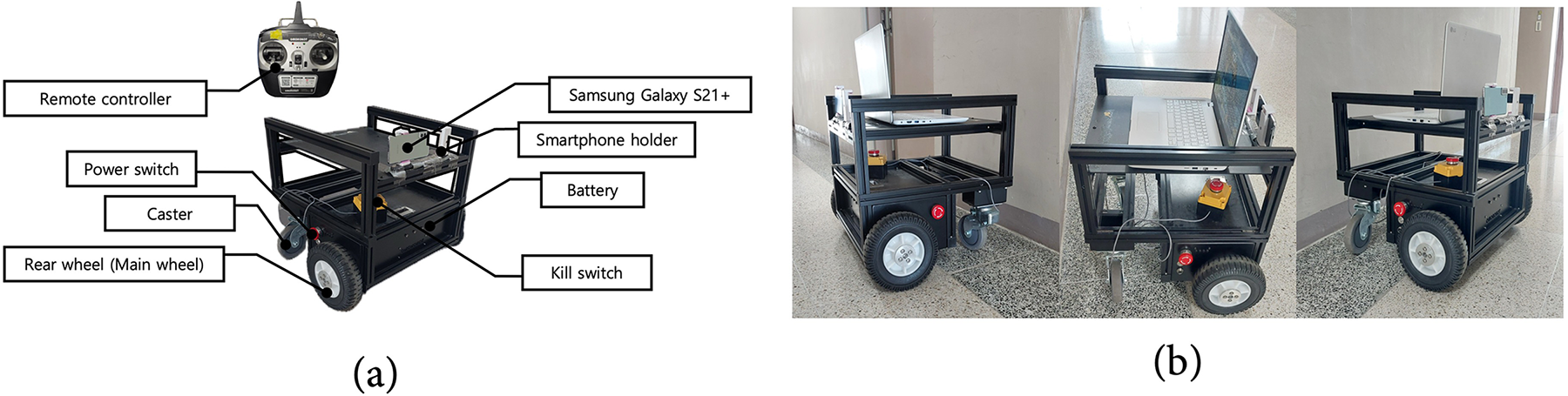
Figure 8: Overview of the R1 V2 experimental robot: (a) Detailed specifications of the experimental robot R1 V2, (b) Experimental setup showing the R1 V2 robot equipped with a smartphone
4.2 Ablation Experiments on Vanishing Point Detection
To evaluate the performance of the proposed algorithm, we performed an ablation study focusing on the vanishing point detection module for precision perspective space detection. For rigorous evaluation, we manually constructed ground truth for the test images. The ground truth for the perspective space was annotated by a single annotator to eliminate inter-annotator variance and ensure consistent application of the guidelines. In this study, the perspective space is defined as: “an axis-aligned rectangle that as tightly as possible encloses the deepest forward traversal region consistent with the dominant vanishing point and direction in large, complex room-scale environments, thereby marking the perspective space that is useful for path finding and obstacle awareness.” Annotation was conducted using an internally developed tool that overlays bounding boxes on images and exports the coordinates in CSV format. For each sample, we record filename, x, y, width, and height, where x and y denote the centroid of the perspective space and width/height are measured in pixels. Access is provided under an agreement that restricts use to non-commercial research and prohibits redistribution, thereby ensuring compliance with ethical guidelines.
Based on this ground truth, we computed confusion matrix-based inference accuracy for the perspective space regions predicted by the method under evaluation and used it as the classification performance metric. In addition, to quantify the agreement between the detected perspective space regions and the ground truth, we designed an evaluation metric, IoP, and applied it in the performance assessment. The IoU metric evaluates the overall overlap between a prediction and the ground truth, but it has limitations for spatial evaluation when region boundaries are ambiguous. Even if the inferred perspective space region is entirely contained within the ground truth, the union area can remain large, yielding a low IoU; likewise, when the predicted region is smaller than the ground truth yet still acceptable as a correct detection, IoU may still be low, complicating fine-grained evaluation. To address this, we propose Intersection over Prediction (IoP), which defines the model’s predicted perspective space region as prediction and computes the proportion of the overlap with the ground truth relative to the prediction area shown in Eq. (14). In addition, to comprehensively assess segmentation performance, we applied IoP to the standard COCO [7] evaluation method and report mAP@ [0.50:0.95] computed over IoP thresholds from 0.50 to 0.95.
The proposed vanishing point detection method integrates ASP (which filters vertical and horizontal boundary noise) Contour (which filters noise in HoughLinesP line detection) and RANSAC (which rejects low-precision candidate vanishing points). Accordingly, the ablation study evaluated performance across combinations in which ASP, Contour, and RANSAC were omitted. For comparison, we summarized the results in Table 4 using accuracy, precision, recall, F1 score, mean IoP, and mAP@ [0.50:0.95]. Fig. 9 visualizes the outcomes of the ablation on vanishing point detection. Cases 1–5 correspond to the respective combinations in which Contour, ASP, and RANSAC were ablated.
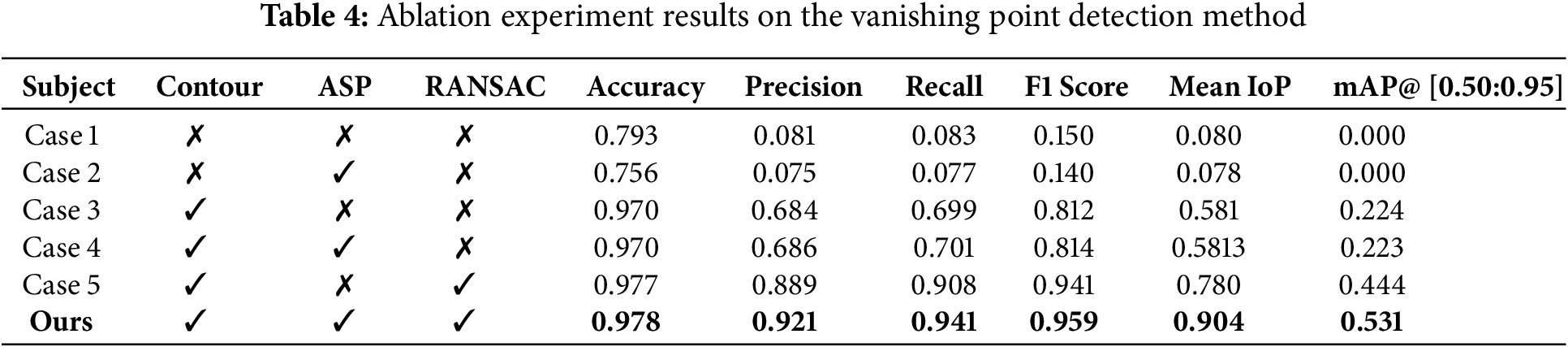
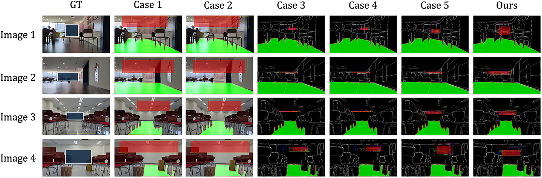
Figure 9: Comparative ablation results for the vanishing point detection method
Through these experiments, the proposed algorithm combining Contour, ASP, and RANSAC achieved F1 score 0.959, mean IoP 0.904, and mAP@ [0.50:0.95] 0.531. It outperformed variants that omitted or only partially incorporated Contour, ASP, or RANSAC. In detail, enabling Contour yielded the largest overall performance gain, followed by ASP and RANSAC, which provided comparable improvements. We attribute this to Contour filtering a substantial amount of noise from the initial HoughLinesP detections used for dimension-wise boundary estimation in geometry-deficient room-scale environments, thereby removing the largest share of noisy data. Subsequently, ASP suppresses excessive vertical/horizontal boundary noise and RANSAC prunes outlier vanishing points, offering additional filtering and secondary gains. Therefore, employing Contour, ASP, and RANSAC together demonstrates that our algorithm achieves precise dimension-wise boundary and vanishing-point detection in geometry-deficient room-scale environments.
4.3 Comparative Evaluation of Multi-Resolution and Fixed-Resolution Sampling
An evaluation is conducted on the multi-resolution sampling method employed for dimension-wise boundary detection in the proposed algorithm. For comparison, we computed the results using fixed-resolution sampling, where the segmentation parameter points per side was set to constant values. In order to make the comparison fair, the vanishing point detection method used for dimension-wise boundary detection included all three algorithms (Contour, ASP, and RANSAC). We evaluated performance using the perspective space regions produced when points per side was individually fixed to 8, 12, 16, 20, 24, 28, and 32. Following Section 4.2, we summarized accuracy, precision, recall, F1 score, mean IoP, and mAP@ [0.50:0.95] based on the ground truth. The numerical results are presented in Table 5, and Fig. 10 visualizes the comparison between multi-resolution and fixed-resolution sampling. In this setup, Cases 1–7 correspond to the respective fixed points per side values.
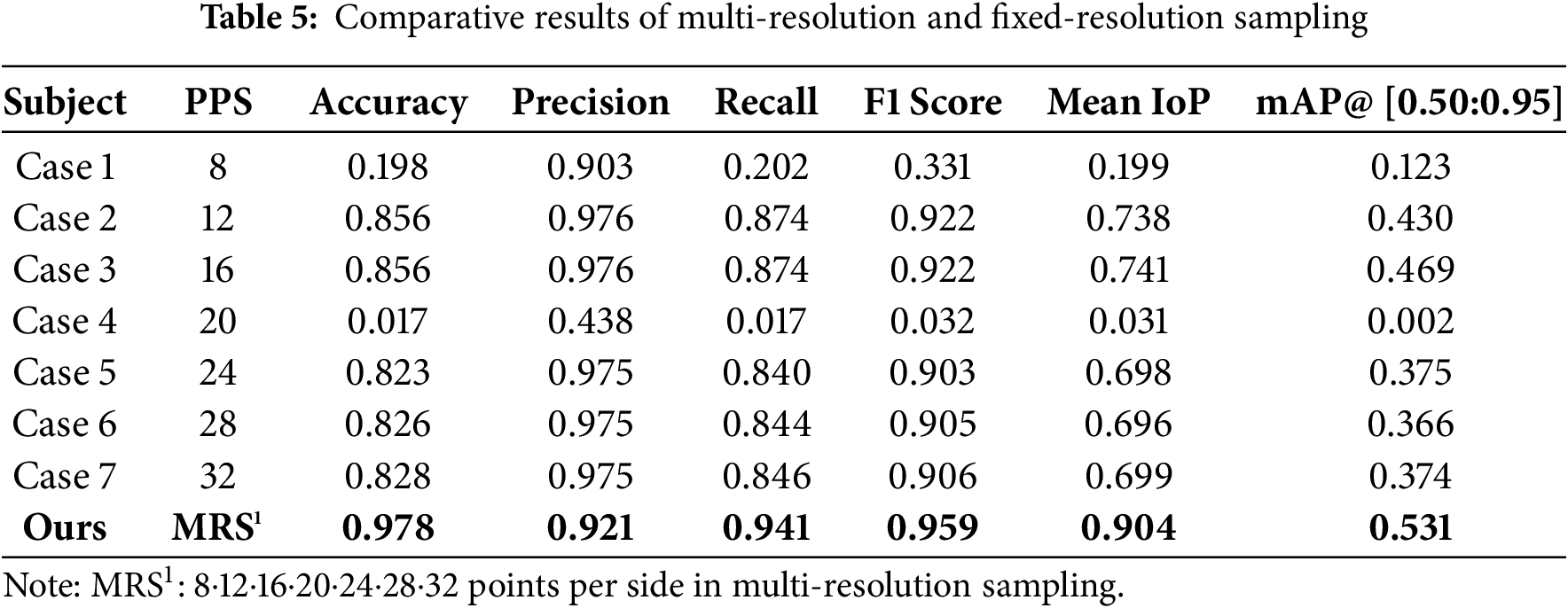
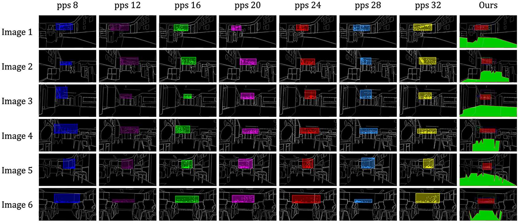
Figure 10: Comparative results for multi-resolution and fixed-resolution sampling
Through these experiments, the multi-resolution sampling method (applying multiple points per side values) outperformed fixed-resolution sampling with a single point per side, yielding an average F1 score improvement of 26.7% and a maximum gain of 92.7%. The mean IoP improved by 36.1% on average, with a maximum gain of 87.3%, and mAP@ [0.50:0.95] improved by 22.5% on average, with a maximum gain of 52.9%. Moreover, when comparing results across specific points per side settings, we observe that increasing points per side does not lead to proportionally higher performance. The results demonstrate that, given the diversity and irregularity of large, complex room-scale environments, using a fixed points per side is not consistently advantageous. Therefore, for general-purpose zero-shot 3D scene understanding in geometry-deficient room-scale environments, the proposed multi-resolution sampling is better suited than fixed-resolution sampling.
4.4 Comparative Evaluation of Precision Perspective Detection with Existing Methods
The proposed algorithm designs a precision perspective detection method built upon monocular depth estimation. Accordingly, we conducted comparative experiments against six existing monocular depth estimation methods and prior research on zero-shot general-purpose 3D mapping. For a fair comparison, the center of each perspective region was fixed at the method’s farthest depth pixel, while the width and height were varied under three settings: P1—center from each baseline; size set to that baseline’s own width and height derived from its top-10% farthest depth rectangular region; P2—center from each baseline, size taken as an oracle from ground truth width and height; P3—center from each baseline; size set to the proposed algorithm’s precision perspective predicted width and height. After generating regions in an identical manner across settings, accuracy, precision, recall, F1@0.5, mean IoP, and mAP@ [0.50:0.95] were computed against ground truth in Section 4.2. Sensitivity(robustness) to region size (P1–P3) was assessed and summarized in Table 6 using the mean, median, TrimMean20, CV, Min, CVaR25, and the 95% CI of the mean.
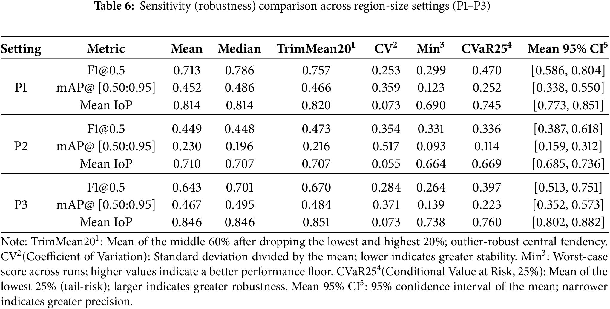
From Table 6, P3 is consistently superior on geometry-consistency indicators. Mean IoP for P3 is 0.846 (95% CI [0.802, 0.882]), exceeding P1 0.814 ( [0.773, 0.851]) and P2 0.710 ( [0.685, 0.736]). The mAP@ [0.50:0.95] under P3 is 0.467 ( [0.352, 0.573]), higher than P1 0.452 ( [0.338, 0.550]) and far above P2 0.230 ( [0.159, 0.312]). In stability terms, CV(IoP) for P3 is 0.073 (on par with P1), while tail robustness is strongest (Min IoP 0.738 vs. 0.690/0.664; CVaR25(IoP) 0.760 vs. 0.745/0.669 for P1/P2). Although P1 attains the highest F1@0.5 (mean 0.713, median 0.786), this reflects a recall-biased operating point and is accompanied by larger dispersion and weaker floor performance on geometry-based metrics (mAP/IoP). By contrast, P3 maintains competitive F1 (mean 0.643, median 0.701) while delivering higher means/medians/TrimMean20 on mAP/IoP, equal or lower CV, and more favorable Min, CVaR25, and Mean 95% CI, indicating the best balance of accuracy and robustness. Accordingly, all subsequent comparisons adopt the P3 protocol—keeping each baseline’s center at its farthest depth pixel while fixing the crop size to our algorithm’s predicted width and height. Following Section 4.4, we evaluate accuracy, precision, recall, F1 score, mean IoP, and mAP@ [0.50:0.95] against the ground truth. Table 7 summarizes the results, and Fig. 11 visualizes the comparative outcomes across the eight methods.
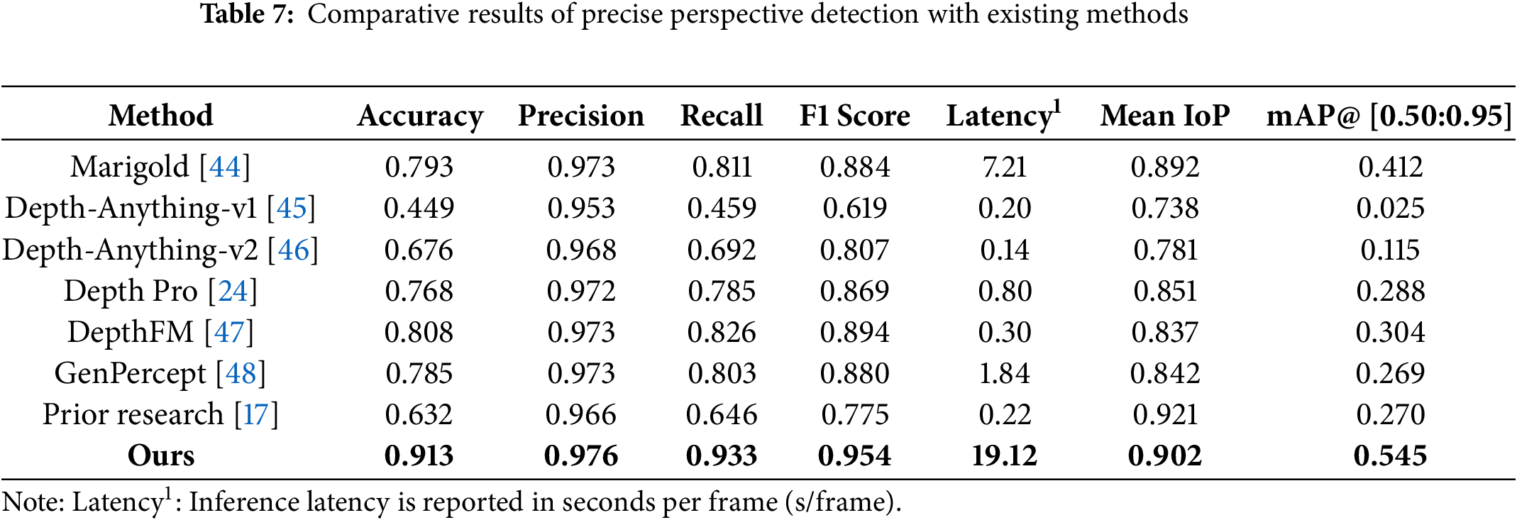
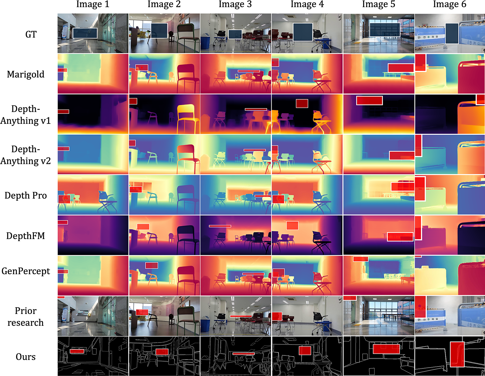
Figure 11: Comparative results of precise perspective detection with existing methods
Across the eight methods compared, our algorithm (augmented with percentile-damping, dynamic scale, and a composite score that fuses the overlap coherence score and depth confidence score) achieved superior results over prior research. Compared to the prior zero-shot, corridor-structured indoor 3D mapping method, the proposed approach achieved improvements of 17.9% in F1 score, and 27.5% in mAP@ [0.50:0.95]. These gains arise from deeply fusing not only single-pixel depth estimates but also geometric cues (such as dimension-wise boundary information and vanishing points) to enable precise perspective detection. Specifically, percentile damping reduces sensitivity to depth outliers; dynamic scale corrects accumulated scale errors across different spaces; and the composite score combining overlap coherence and depth confidence jointly optimizes the reliability and consistency of the inferred precision perspective space regions. Furthermore, even under extreme scenarios—such as indoor environments with strong illumination and light reflections (e.g., Image 5 in Fig. 11) or severe occlusions caused by obstacles (e.g., Image 6 in Fig. 11)—the proposed algorithm demonstrated more accurate and robust performance compared to other existing methods. The inference latency of our proposed algorithm is longer than that of other depth estimation baselines. However, this computational cost remains acceptable in large-scale environments where geometric cues are insufficient. The proposed method consistently delivers more reliable and precise obstacle recognition and 3D reconstruction. Although the processing time is comparatively longer than that of other methods used for performance validation, the algorithm maintains practical applicability in geometry-deficient, large and complex room-scale environments where walls or uniformly arranged structures are insufficient, as accuracy and robustness are prioritized over frame-by-frame speed.
4.5 Comparative Evaluation of Floor Mask Extraction with Existing Methods
To evaluate the performance of the proposed floor mask extraction method, comparative experiments were conducted with four existing segmentation algorithms and one prior study’s floor detection module based on corridor structure. Two of the segmentation models are text prompt-based; both used the keyword “floor” as input to the pre-trained model to generate corresponding floor masks. The third method is a coordinate-based segmentation model, which receives precise pixel locations of the floor manually defined on the input image to generate floor masks. Additionally, the floor detection module of the prior corridor-structure-based approach was included for comparison. For all five methods, confusion matrices were computed, and classification metrics—accuracy, precision, recall, and F1 score—were reported, as shown in Table 8. Ground truth floor masks were also constructed to calculate Intersection over Union (IoU) and mean Average Precision (mAP@ [0.50:0.95]). Unlike precision perspective detection metrics like IoP, floor mask extraction allows a clearer area-wise comparison against ground truth. It also yields less inference variability, making IoU-based metrics more suitable for evaluation. Therefore, mAP@ [0.50:0.95] was computed using IoU to evaluate the floor mask extraction results. Fig. 12 shows the visual outcomes of the comparative floor mask detection experiments.
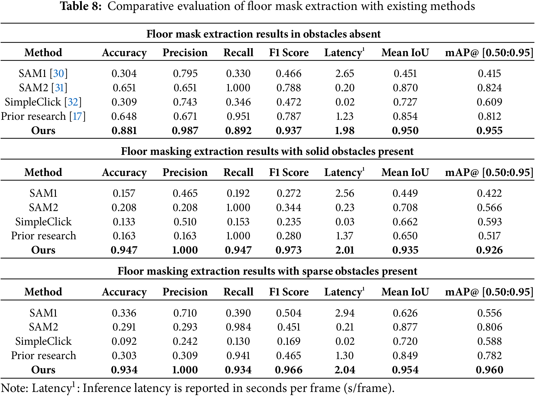
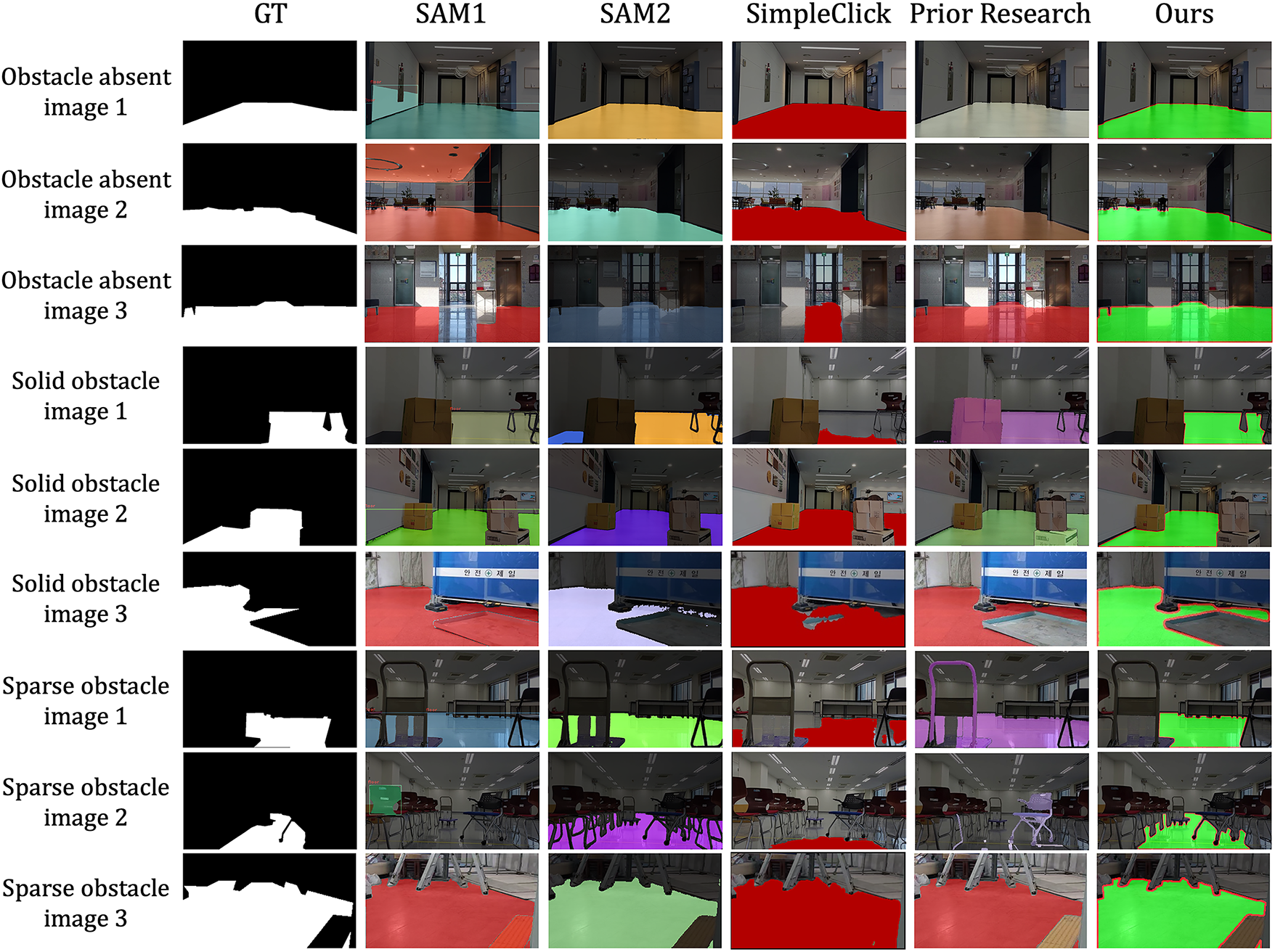
Figure 12: Comparative results floor mask extraction results with existing methods
Through the above experiments, the proposed algorithm demonstrated consistently superior performance across all scenarios: environments without obstacles, with solid obstacles, and with sparse obstacles. In obstacle absent environments, the algorithm achieved a mean IoU of 0.950 and mAP@ [0.50:0.95] of 0.955. These results surpassed those of SimpleClick, which showed a mean IoU of 0.727 and mAP@ [0.50:0.95] of 0.609. Although SAM2 achieved a perfect recall of 1.000, its precision was only 0.651, yielding an f1 score of 0.788. In contrast, the proposed algorithm achieved a precision of 0.987, recall of 0.892, and an f1 score of 0.937. This indicates its robustness in mitigating the over-segmentation issues observed in SAM-based methods. In environments with solid obstacles, the proposed method achieved a mean IoU of 0.935 and mAP@ [0.50:0.95] of 0.926. This outperformed SAM2, which recorded a mean IoU of 0.708 and mAP@ [0.50:0.95] of 0.566. It also demonstrated balanced classification metrics with an accuracy of 0.947, precision of 1.000, recall of 0.947, and an f1 score of 0.973. For environments with sparse obstacles, the proposed algorithm achieved the highest f1 score of 0.966, mean IoU of 0.954, and mAP@ [0.50:0.95] of 0.960. In comparison, SAM2, the second-best performer in terms of IoU, achieved a mean IoU of 0.877 and mAP@ [0.50:0.95] of 0.806. As shown in Fig. 12, other methods often exhibited boundary omissions (under-segmentation) or leakage (over-segmentation) around obstacles. In contrast, the proposed algorithm-maintained boundary continuity and effectively suppressed mask leakage near obstacle tangents. This was particularly evident in environments with sparse obstacles, where existing approaches tended to over-segment the floor due to high geometric complexity. Such over-segmentation can lead to confusion in identifying traversable regions. The proposed method reliably suppressed this over-segmentation and accurately detected precise floor masks, even in the presence of sparse obstacles. Moreover, even under extreme scenarios—such as indoor environments with strong illumination and light reflections (e.g., Obstacle absent image 3 in Fig. 12) or severe occlusions caused by obstacles (e.g., Solid obstacle image 3 and Sparse obstacle image 3 in Fig. 12)—the proposed algorithm extracted more accurate and robust floor mask compared to other existing methods.
4.6 Comparative Evaluation of Obstacle Recognition and Classification with Existing Methods
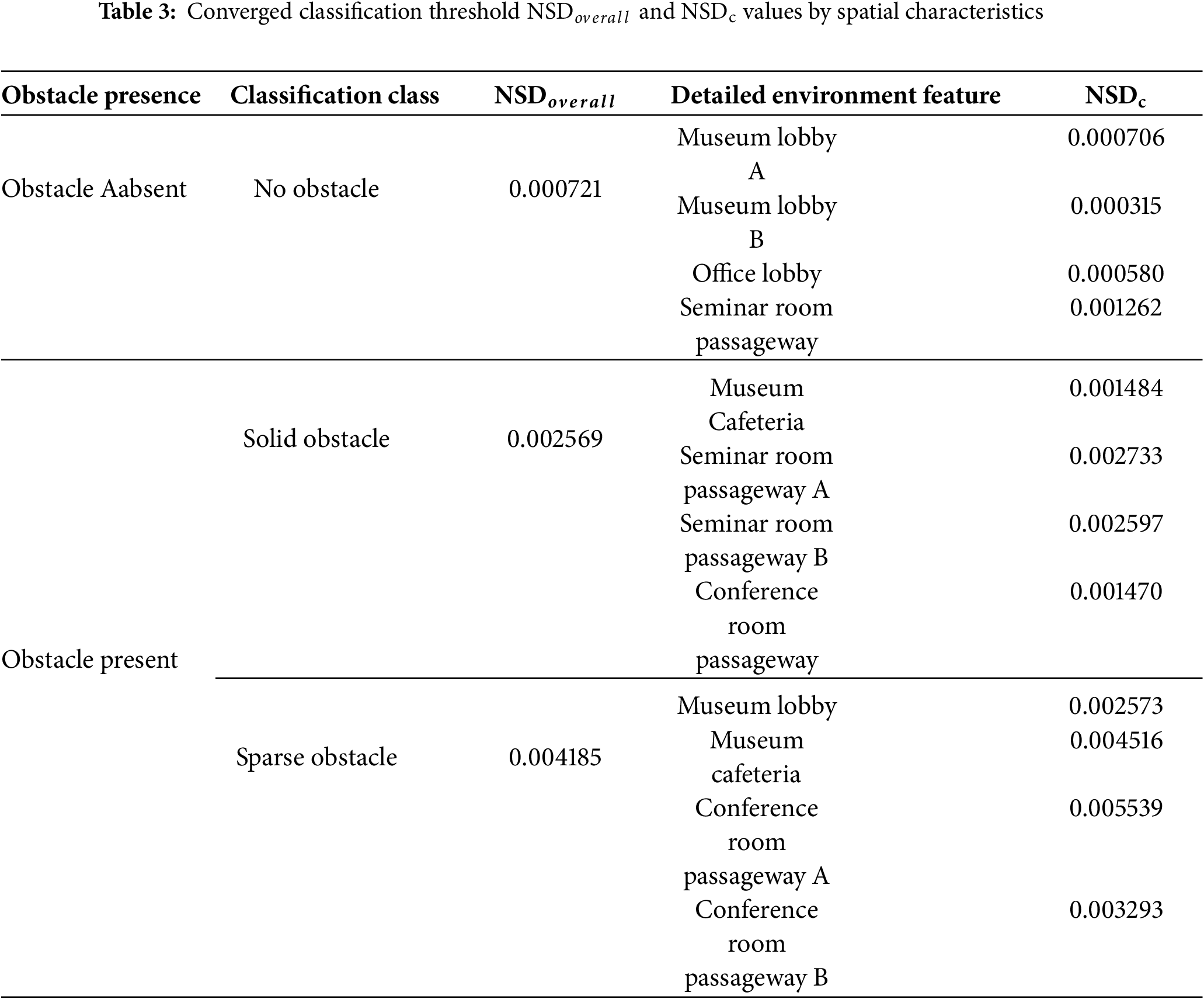
This experiment verifies the performance of obstacle presence recognition and obstacle type classification in large, complex room-scale environments. To validate the proposed algorithm, we tested its classification accuracy using the converged thresholds of three
The results confirm that the proposed
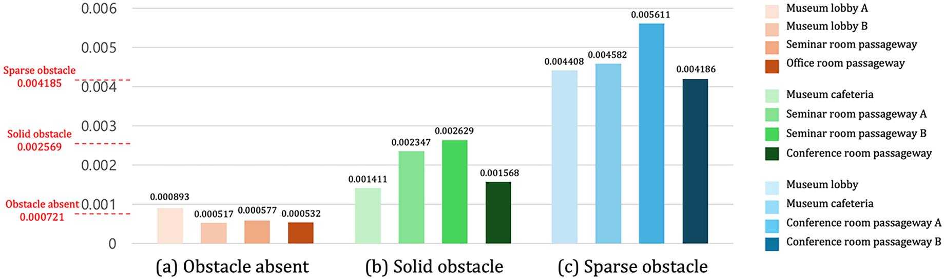
Figure 13: Obstacle recognition and classification across test environments based on
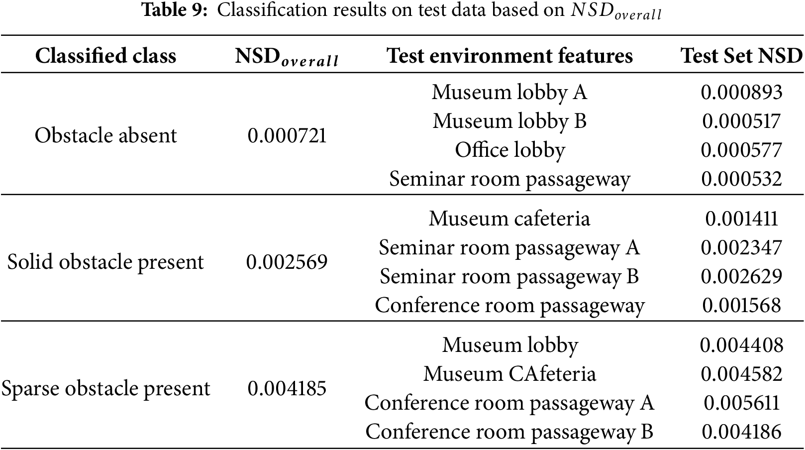
For additional validation, the proposed algorithm’s performance was evaluated using classification metrics. Its performance was compared against existing methods that detect obstacles using pretrained models. To compute the classification metrics for the proposed method, the test dataset was categorized into three sets: obstacle absent, solid obstacle present, and sparse obstacle present. A total of 45 samples were randomly selected from each set, representing half of the data from each environment. The NSD values obtained from these sampled frames were then used to construct the evaluation dataset. Classification was performed using these NSD values, and prediction results were compared with ground truth labels. The accuracy of inference was then summarized using standard classification metrics.
For comparative evaluation, three text-prompt based segmentation models and prior depth–segmentation fusion method was tested. The segmentation models were given the prompt “object” as input, following their pretrained setup. Obstacle recognition performance across all five methods was measured using confusion matrices. Table 10 summarizes the results in terms of accuracy, precision, recall, and F1 score.
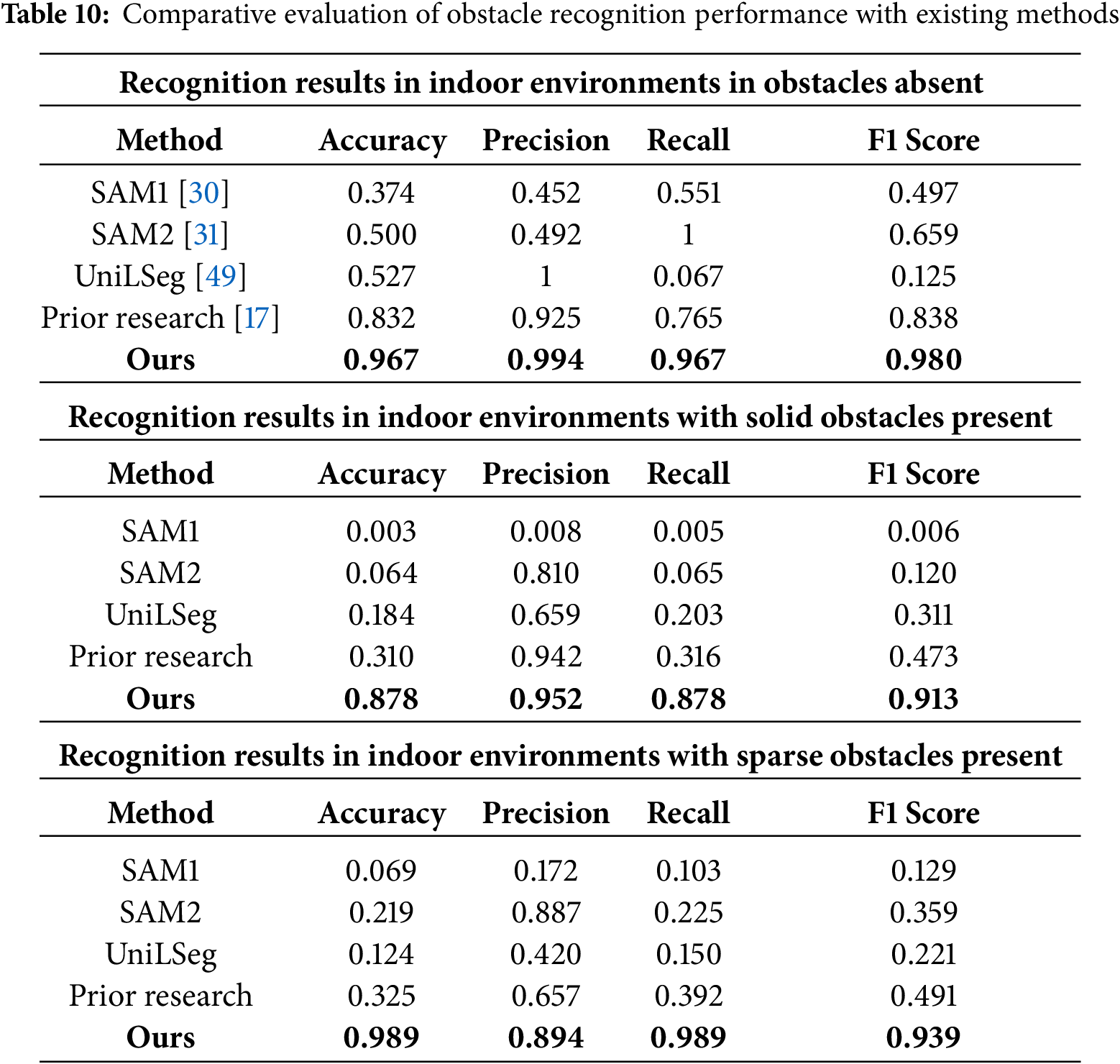
Through the comparative analysis of five methods, the proposed algorithm consistently outperformed across all scenarios, demonstrating the best precision-recall balance and highest F1 scores. In obstacle absent environments, the proposed method achieved a precision of 0.994 and recall of 0.967, resulting in an F1 score of 0.980. This represents an improvement of more than 0.14 in F1 score over the next best method, which achieved an F1 score of 0.838. Although SAM2 achieved a recall of 1.000, it suffered from over-segmentation, yielding a precision of 0.492 and an F1 score of only 0.659. In contrast, our method effectively suppressed over-segmentation while maintaining recall, achieving the most stable performance with an accuracy of 0.967. In environments with solid obstacles, the proposed method reached a precision of 0.952 and recall of 0.878, achieving an F1 score of 0.913. This demonstrates a substantial improvement, as the proposed method achieved an F1 score that is 0.44 higher than the best result among existing methods, which recorded an F1 score of 0.473. SAM2 showed a low recall of 0.065, despite a relatively high precision of 0.810, resulting in a F1 score of 0.120 due to frequent detection failures. In contrast, our algorithm significantly reduced detection failures, achieving an accuracy of 0.878. In environments containing sparse obstacles, our algorithm achieved a precision of 0.894 and recall of 0.989, yielding an F1 score of 0.939. This represents an improvement of 0.448 over the next best method, which achieved an F1 score of 0.491.
These results confirm that the proposed algorithm, which employs a robust three-layer robust 3D map-reconstruction, accurately estimates
This study reconstructs insufficient dimensional spatial data to achieve accurate 3D map recovery in geometry-deficient room-scale environments. The proposed algorithm recognizes and classifies not only solid obstacles but also skeleton-type sparse obstacles, such as chairs and desks. It also identifies floor masks and precision perspective spaces to generate key data for 3D spatial mapping. The main contributions of this study are as follows: First, by leveraging a zero-shot vision-based general AI approach, it enables 3D scene understanding without large-scale label retraining. This allows for immediate interpretation of large, complex room-scale environments. Second, the algorithm hierarchically fuses three layers: dimension-wise boundary extraction, precision perspective detection, and floor mask extraction. This fusion enables 3D spatial mapping and obstacle classification, even in geometry-deficient room-scale environments. Third, the system uses only a low-cost monocular RGB camera, offering a practical alternative to expensive LiDAR systems. To validate the algorithm, we conducted experiments on datasets collected from lobbies, seminar rooms, conference halls, cafeterias, and museums. In precision perspective detection, the proposed method achieved an F1 score of 0.959 and an average IoP of 0.904, outperforming prior approaches. For floor mask extraction, it achieved an F1 score of 0.931 and IoU of 0.928 in obstacle absent environments. In solid obstacle environments, it recorded an F1 score of 0.971 and IoU of 0.914. In sparse obstacle environments, it showed an F1 score of 0.956 and IoU of 0.937. In obstacle recognition and classification, the F1 score reached 0.980 in obstacle absent environments. It achieved 0.913 with solid obstacles, and 0.939 with sparse obstacles, demonstrating precision and reliability. These results support the practical expansion of this method to indoor applications such as service robot navigation, smart city infrastructure, and autonomous driving.
Acknowledgement: The authors would like to sincerely express their advisor, Prof. Junho Ahn, for insightful guidance and continued support. The authors also appreciate the constructive discussions and encouragement received from colleagues and peers, which provided meaningful inspiration during the development of this work.
Funding Statement: This work was supported by Kyonggi University Research Grant 2025.
Author Contributions: The authors confirm contribution to the paper as follows: study conception and design: Taehoon Kim, Sehun Lee, Junho Ahn; data collection: Taehoon Kim, Sehun Lee; analysis and interpretation of results: Taehoon Kim, Sehun Lee, Junho Ahn; draft manuscript preparation: Taehoon Kim. All authors reviewed the results and approved the final version of the manuscript.
Availability of Data and Materials: The data used in this study, including ground truth annotations, are available from the corresponding author (Junho Ahn) or the first author (Taehoon Kim) upon request via email.
Ethics Approval: Not applicable.
Conflicts of Interest: The authors declare no conflicts of interest to report regarding the present study.
References
1. Domestic Service robots market size & share analysis—growth trends & forecasts (2025–2030). 2025 [cited 2025 Aug 1]. Available from: https://www.mordorintelligence.com/industry-reports/domestic-service-robots-market?utm. [Google Scholar]
2. Xiao X, Xu Z, Datar A, Warnell G, Stone P, Damanik JJ, et al. Autonomous ground navigation in highly constrained spaces: lessons learned from the third BARN challenge at ICRA 2024 [competitions]. IEEE Robot Autom Mag. 2024;31(3):197–204. doi:10.1109/mra.2024.3427891. [Google Scholar] [CrossRef]
3. Lafuente-Arroyo S, Maldonado-Bascón S, Gómez-Moreno H, Alén-Cordero C. Segmentation in corridor environments: combining floor and ceiling detection. In: Proceedings of the Iberian Conference on Pattern Recognition and Image Analysis 2019; 2019 Jul 1; Madrid, Spain. p. 485–96. doi:10.1007/978-3-030-31321-0_42. [Google Scholar] [CrossRef]
4. Chen P, Zhao X, Zeng L, Liu L, Liu S, Sun L, et al. A review of research on SLAM technology based on the fusion of LiDAR and vision. Sensors. 2025;25(5):1447. doi:10.3390/s25051447. [Google Scholar] [PubMed] [CrossRef]
5. Tran B, Attorney P. The cost of self-driving technology: how much do AV components really cost? (market breakdown) [Internet]. 2025 [cited 2025 Aug 1]. Available from: https://patentpc.com/blog/the-cost-of-self-driving-technology-how-much-do-av-components-really-cost-market-breakdown. [Google Scholar]
6. Godard C, Mac Aodha O, Brostow GJ. Unsupervised monocular depth estimation with left-right consistency. In: Proceedings of the 2017 IEEE Conference on Computer Vision and Pattern Recognition (CVPR); 2017 Jul 21–26; Honolulu, HI, USA. p. 6602–11. doi:10.1109/CVPR.2017.699. [Google Scholar] [CrossRef]
7. Lin TY, Maire M, Belongie S, Hays J, Perona P, Ramanan D, et al. Microsoft COCO: common objects in context. In: Proceedings of the Computer Vision—ECCV 2014; 2014 Sep 6–12; Zurich, Switzerland. p. 740–55. doi:10.1007/978-3-319-10602-1_48. [Google Scholar] [CrossRef]
8. Zhang H, Li F, Liu S, Zhang L, Su H, Zhu J, et al. DINO: dETR with improved DeNoising anchor boxes for end-to-end object detection. arXiv:2203.03605. 2022. doi:10.48550/arXiv.2203.03605. [Google Scholar] [CrossRef]
9. Fan Z, Mei W, Liu W, Chen M, Qiu Z. I-DINO: high-quality object detection for indoor scenes. Electronics. 2024;13(22):4419. doi:10.3390/electronics13224419. [Google Scholar] [CrossRef]
10. Kim D, Kim C, Ahn J. Vision-based recognition algorithm for up-to-date indoor digital map generations at damaged buildings. Comput Mater Contin. 2022;72(2):2765–81. doi:10.32604/cmc.2022.025116. [Google Scholar] [CrossRef]
11. Radford A, Kim JW, Hallacy C, Ramesh A, Goh G, Agarwal S, et al. Learning transferable visual models from natural language supervision. arXiv:2103.00020. 2021. doi:10.48550/arXiv.2103.00020. [Google Scholar] [CrossRef]
12. Chen T, Kornblith S, Norouzi M, Hinton G. A simple framework for contrastive learning of visual representations. arXiv:2002.05709. 2020. doi:10.48550/arXiv.2002.05709. [Google Scholar] [CrossRef]
13. Rombach R, Blattmann A, Lorenz D, Esser P, Ommer B. High-resolution image synthesis with latent diffusion models. In: Proceedings of the 2022 IEEE/CVF Conference on Computer Vision and Pattern Recognition (CVPR); 2022 Jun 18–24; New Orleans, LA, USA. p. 10674–85. doi:10.1109/CVPR52688.2022.01042. [Google Scholar] [CrossRef]
14. Oord A, Vinyals O, Kavukcuoglu K. Neural discrete representation learning. arXiv:1711.00937. 2017. doi:10.48550/arXiv.1711.00937. [Google Scholar] [CrossRef]
15. Alayrac JB, Donahue J, Luc P, Miech A, Barr I, Hasson Y, et al. Flamingo: a visual language model for few-shot learning. arXiv:2204.14198. 2022. doi:10.48550/arXiv.2204.14198. [Google Scholar] [CrossRef]
16. Li C, Gan Z, Yang Z, Yang J, Li L, Wang L, et al. Multimodal foundation models: from specialists to general-purpose assistants. Found Trends Comput Graph Vis. 2024;16(1–2):1–214. doi:10.1561/0600000110. [Google Scholar] [CrossRef]
17. Lee S, Kim T, Ahn J. Zero-shot based spatial AI algorithm for up-to-date 3D vision map generations in highly complex indoor environments. Comput Mater Contin. 2025;84(2):3623–48. doi:10.32604/cmc.2025.063985. [Google Scholar] [CrossRef]
18. Zhang Z, Zhang Y, Li Y, Wu L. Review of monocular depth estimation methods. J Electron Imag. 2025;34(2):20901. doi:10.1117/1.jei.34.2.020901. [Google Scholar] [CrossRef]
19. Shi X, Chen Z, Wang H, Yeung DY, Wong WK, Woo WC. Convolutional LSTM network: a machine learning approach for precipitation nowcasting. arXiv:1506.04214. 2015. doi:10.48550/arXiv.1506.04214. [Google Scholar] [CrossRef]
20. Vaswani A, Shazeer N, Parmar N, Uszkoreit J, Jones L, Gomez AN, et al. Attention is all you need. arXiv:1706.03762. 2017. doi:10.48550/arXiv.1706.03762. [Google Scholar] [CrossRef]
21. Silberman N, Hoiem D, Kohli P, Fergus R. Indoor segmentation and support inference from RGBD images. In: Proceedings of the Computer Vision—ECCV 2012; 2012 Oct 7–13; Florence, Italy. p. 746–60. doi:10.1007/978-3-642-33715-4_54. [Google Scholar] [CrossRef]
22. Geiger A, Lenz P, Stiller C, Urtasun R. The KITTI vision benchmark suite: depth evaluation [Internet]. 2025 [cited 2025 Aug 1]. Available from: http://www.cvlibs.net/datasets/kitti/eval_depth_all.php. [Google Scholar]
23. Cordts M, Omran M, Ramos S, Rehfeld T, Enzweiler M, Benenson R, et al. The cityscapes dataset for semantic urban scene understanding. In: Proceedings of the 2016 IEEE Conference on Computer Vision and Pattern Recognition (CVPR); 2016 Jun 27–30; Las Vegas, NV, USA. p. 3213–23. doi:10.1109/CVPR.2016.350. [Google Scholar] [CrossRef]
24. Bochkovskii A, Delaunoy A, Germain H, Santos M, Zhou Y, Richter SR, et al. Depth pro: sharp monocular metric depth in less than a second. arXiv:2410.02073. 2024. doi:10.48550/arXiv.2410.02073. [Google Scholar] [CrossRef]
25. Goodfellow I, Pouget-Abadie J, Mirza M, Xu B, Warde-Farley D, Ozair S, et al. Generative adversarial networks. Commun ACM. 2020;63(11):139–44. doi:10.1145/3422622. [Google Scholar] [CrossRef]
26. Kingma DP, Welling M. Auto-encoding variational Bayes. arXiv:1312.6114. 2013. doi:10.48550/arXiv.1312.6114. [Google Scholar] [CrossRef]
27. Liu Z, Lin Y, Cao Y, Hu H, Wei Y, Zhang Z, et al. Swin transformer: hierarchical vision transformer using shifted windows. In: Proceedings of the 2021 IEEE/CVF International Conference on Computer Vision (ICCV); 2021 Oct 10–17; Montreal, QC, Canada. p. 9992–10002. doi:10.1109/ICCV48922.2021.00986. [Google Scholar] [CrossRef]
28. Bhat SF, Alhashim I, Wonka P. AdaBins: depth estimation using adaptive bins. arXiv:2011.14141. 2011. doi:10.48550/arXiv.2011.14141. [Google Scholar] [CrossRef]
29. Li Z, Wang X, Liu X, Jiang J. BinsFormer: revisiting adaptive bins for monocular depth estimation. IEEE Trans Image Process. 2024;33:3964–76. doi:10.1109/TIP.2024.3416065. [Google Scholar] [PubMed] [CrossRef]
30. Kirillov A, Mintun E, Ravi N, Mao H, Rolland C, Gustafson L, et al. Segment anything. In: Proceedings of the 2023 IEEE/CVF International Conference on Computer Vision (ICCV); 2023 Oct 1–6; Paris, France. p. 3992–4003. doi:10.1109/ICCV51070.2023.00371. [Google Scholar] [CrossRef]
31. Ravi N, Gabeur V, Hu YT, Hu R, Ryali C, Ma T, et al. Sam 2: segment anything in images and videos. arXiv:2408.00714. 2024. doi:10.48550/arXiv.2408.00714. [Google Scholar] [CrossRef]
32. Liu Q, Xu Z, Bertasius G, Niethammer M. SimpleClick: interactive image segmentation with simple vision transformers. In: Proceedings of the 2023 IEEE/CVF International Conference on Computer Vision (ICCV); 2023 Oct 1–6; Paris, France. p. 22233–43. doi:10.1109/ICCV51070.2023.02037. [Google Scholar] [PubMed] [CrossRef]
33. Quattoni A, Torralba A. Recognizing indoor scenes. In: Proceedings of the 2009 IEEE Conference on Computer Vision and Pattern Recognition; 2009 Jun 20–25; Miami, FL, USA. p. 413–20. doi:10.1109/CVPR.2009.5206537. [Google Scholar] [CrossRef]
34. Yu LF, Yeung SK, Tang CK, Terzopoulos D, Chan TF, Osher SJ. Make it home: automatic optimization of furniture arrangement. ACM Trans Graph. 2011;30(4):1–12. doi:10.1145/2010324.1964981. [Google Scholar] [CrossRef]
35. Di X, Yu P. Deep reinforcement learning for producing furniture layout in indoor scenes. arXiv:2101.07462. 2021. doi:10.48550/arXiv.2101.07462. [Google Scholar] [CrossRef]
36. Wang Y, McConachie D, Berenson D. Tracking partially-occluded deformable objects while enforcing geometric constraints. In: Proceedings of the 2021 IEEE International Conference on Robotics and Automation (ICRA); 2021 May 30–Jun 5; Xi’an, China. p. 14199–205. doi:10.1109/ICRA48506.2021.9561012. [Google Scholar] [CrossRef]
37. Kass M, Witkin A, Terzopoulos D. Snakes: active contour models. Int J Comput Vis. 1988;1(4):321–31. doi:10.1007/BF00133570. [Google Scholar] [CrossRef]
38. Kiryati N, Eldar Y, Bruckstein AM. A probabilistic Hough transform. Pattern Recognit. 1991;24(4):303–16. doi:10.1016/0031-3203(91)90073-E. [Google Scholar] [CrossRef]
39. OpenCV.org. Hough line transform [Internet]. 2025 [cited 2025 Aug 1]. Available from: https://docs.opencv.org/3.4/d9/db0/tutorial_hough_lines.html. [Google Scholar]
40. FacebookResearch. Segment anything [Internet]. 2023 [cited 2025 Aug 1]. Available from: https://github.com/facebookresearch/segment-anything/blob/6fdee8f2727f4506cfbbe553e23b895e27956588/segment_anything/automatic_mask_generator.py#L39. [Google Scholar]
41. Fischler MA, Bolles RC. Random sample consensus: a paradigm for model fitting with applications to image analysis and automated cartography. Read Comput Vis. 1987:726–40. doi:10.1016/B978-0-08-051581-6.50070-2. [Google Scholar] [CrossRef]
42. Douglas DH, Peucker TK. Algorithms for the reduction of the number of points required to represent a digitized line or its caricature. Cartographica. 1973;10(2):112–22. doi:10.3138/fm57-6770-u75u-7727. [Google Scholar] [CrossRef]
43. Omorobot. Omorobot.com/r1v2 [Internet]. 2025 [cited 2025 Aug 1]. Available from: https://www.omorobot.com/r1v2/. [Google Scholar]
44. Ke B, Obukhov A, Huang S, Metzger N, Daudt RC, Schindler K. Repurposing diffusion-based image generators for monocular depth estimation. In: Proceedings of the 2024 IEEE/CVF Conference on Computer Vision and Pattern Recognition (CVPR); 2024 Jun 16–22; Seattle, WA, USA. p. 9492–502. doi:10.1109/CVPR52733.2024.00907. [Google Scholar] [CrossRef]
45. Yang L, Kang B, Huang Z, Xu X, Feng J, Zhao H. Depth anything: unleashing the power of large-scale unlabeled data. In: Proceedings of the 2024 IEEE/CVF Conference on Computer Vision and Pattern Recognition (CVPR); 2024 Jun 16–22; Seattle, WA, USA. p. 10371–81. doi:10.1109/CVPR52733.2024.00987. [Google Scholar] [CrossRef]
46. Yang L, Kang B, Huang Z, Zhao Z, Xu X, Feng J, et al. Depth anything V2. arXiv:2406.09414. 2024. doi:10.48550/arXiv.2406.09414. [Google Scholar] [CrossRef]
47. Gui M, Schusterbauer J, Prestel U, Ma P, Kotovenko D, Grebenkova O, et al. DepthFM: fast generative monocular depth estimation with flow matching. Proc AAAI Conf Artif Intell. 2025;39(3):3203–11. doi:10.1609/aaai.v39i3.32330. [Google Scholar] [CrossRef]
48. Xu G, Ge Y, Liu M, Fan C, Xie K, Zhao Z, et al. What matters when repurposing diffusion models for general dense perception tasks? arXiv:2403.06090. 2024. doi:10.48550/arXiv.2403.06090. [Google Scholar] [CrossRef]
49. Liu Y, Zhang C, Wang Y, Wang J, Yang Y, Tang Y. Universal segmentation at arbitrary granularity with language instruction. In: Proceedings of the 2024 IEEE/CVF Conference on Computer Vision and Pattern Recognition (CVPR); 2024 Jun 16–22; Seattle, WA, USA. p. 3459–69. doi:10.1109/CVPR52733.2024.00332. [Google Scholar] [CrossRef]
Cite This Article
 Copyright © 2026 The Author(s). Published by Tech Science Press.
This work is licensed under a Creative Commons Attribution 4.0 International License , which permits unrestricted use, distribution, and reproduction in any medium, provided the original work is properly cited.
 Downloads
 Citation Tools