Engine Failure Prediction on Large-Scale CMAPSS Data Using Hybrid Feature Selection and Imbalance-Aware Learning

1  Introduction

Predictive Maintenance (PdM) is a crucial component of Industry 4.0, enabling companies to keep machines running longer while reducing unexpected breakdowns and associated costs [1]. By predicting the Remaining Useful Life (RUL) or detecting failures before they occur, PdM shifts maintenance from reactive or fixed schedules to condition-based actions [2]. However, even with the large amount of sensor data available in modern industries, three key problems still limit the strength of PdM models: insufficient failure data, an imbalance between healthy and faulty cases and the difficulty of selecting the right features [3]. Failures are rare, so datasets typically have only a small number of faulty examples compared to thousands of regular cycles, which prompts models to focus on the majority class [4]. Additionally, the high-frequency sensors generate large amounts of complex, noisy signals, necessitating the selection of a smaller set of valuable features to enhance clarity, speed, and reliability [5]. These problems are exacerbated by the scarcity of failure cases, which makes it harder to test models properly and confirm that results are trustworthy [4].

Recent work has focused on deep learning methods such as Long Short-Term Memory (LSTMs), Gated Recurrent Units (GRUs), and Convolutional Neural Networks (CNNs), which can capture complex temporal patterns in sensor data [6]. These models achieve high accuracy by learning how systems degrade [7], but they are often treated as black boxes and usually lack modular pipelines that support reproducibility or real-world use [8]. In addition, most studies have placed more emphasis on accuracy while paying less attention to explainability, efficiency and solutions for class imbalance, which limits their value in industrial settings [9]. This gap highlights the need for PdM frameworks that combine the predictive strength of deep learning with clarity, practical efficiency, and strong validation In parallel, prescriptive maintenance studies formalize decision rules, inspection strategies and reliability-aware scheduling that convert predictions into actions, offering a template for linking RUL and calibrated risk to maintenance policies [10].

This study addresses that need by presenting a hybrid ensemble pipeline designed for real-world use in fields such as aerospace and manufacturing [10]. Unlike earlier work that handles feature design, model training and testing as separate tasks, the workflow brings them together into a single process [5]. It combines advanced preprocessing with strong feature selection methods, such as variance thresholding, recursive elimination and tree-based importance, alongside a stacked LSTM–GRU model for sequential data. Classical models, such as logistic regression and Extreme Gradient Boosting (XGBoost), are tested for a fair comparison, and the feature selection ensemble is used as a baseline to assess the impact of feature reduction on performance. To handle imbalance, the pipeline uses RandomOverSampler and class-weighted losses [11]. For reliability, it uses stratified and time-based splits, nested cross-validation, bootstrap confidence intervals, and nonparametric significance tests [4]. For Interpretability, both global and local tools are used, including permutation importance, SHapley Additive exPlanations (SHAP) and Local Interpretable Model-agnostic Explanations (LIME), which help highlight the key drivers of system failures [12]. Additionally, inference speed and resource utilization are measured to confirm that the pipeline is efficient enough for deployment [13].

By bringing these parts together, this research makes three main contributions. First, it demonstrates a scalable approach to transforming large, partially labelled sensor data into balanced, useful feature sets [14]. Second, it proves that hybrid feature selection with a stacked LSTM–GRU improves early warning accuracy compared to classical models [15]. Third, it provides a practical blueprint that includes explainability, strong statistical checks, and performance profiling for real deployment [16]. Overall, these advances deliver a PdM framework that is robust, interpretable, and efficient, helping accelerate the transition from research to industrial use [17].

Motivation and Research Objectives:

Despite the promise of PdM in improving asset availability and reducing downtime, its adoption is limited by scarce and imbalanced failure data, noisy high-dimensional signals and black-box deep models with limited Interpretability. Many studies emphasize accuracy while overlooking transparency, validation and reproducibility, which hinders deployment in safety-critical domains. To close this gap, this research pursues three objectives:

•   RO1: Develop a dual-task PdM system that combines Remaining Useful Life (RUL) regression with early-warning classification.

•   RO2: Design an interpretable and imbalance-aware temporal learning framework with hybrid feature selection and robust resampling.

•   RO3: Ensure deployment-readiness through rigorous evaluation and explainability using SHAP, LIME and permutation importance.

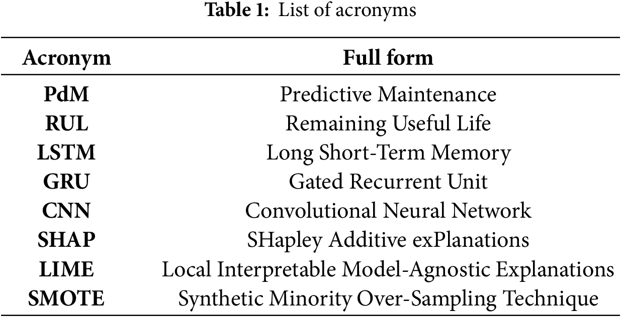
Table 1 provides the full forms and definitions of all acronyms used throughout the manuscript.

2  Literature Review

Early studies on PdM have relied on process control charts and simple classifiers applied to narrow datasets, which limits their ability to capture complex degradation patterns [6]. The release of the NASA CMAPSS turbofan benchmark marked a turning point, becoming the most widely studied RUL dataset and driving a surge in deep learning models [18]. However, many CMAPSS-based works still rely on single-split evaluations, which can lead to overfitting and limit generalization [19]. A central challenge also lies in handling class imbalance, since failure events are far rarer than regular operation. While SMOTE has improved minority recall, it may introduce noise, prompting newer variants such as the Distance-based Extended Synthetic Minority Over-Sampling Technique (Distance-ExtSMOTE), the Dirichlet-based Extended Synthetic Minority Over-Sampling Technique (Dirichlet-ExtSMOTE), and the Dirichlet-based Extended Synthetic Minority Over-Sampling Technique (BGMM-SMOTE) that better preserve class boundaries [20]. Hybrid approaches that combine oversampling, cost-sensitive learning and ensembles often outperform single remedies [21], although most PdM studies still benchmark imbalance methods in isolation rather than against algorithmic alternatives, such as class-weighted or focal loss.

Beyond imbalance, feature selection has progressed from univariate filters to model-aware methods [22]. Mutual information remains popular for improving efficiency, while wrappers such as Recursive Feature Elimination (RFE) provide finer discrimination at a higher computational cost [23]. Explainable tools, such as SHAP, have further bridged the gap between interpretation and selection, enabling the removal of redundant features while retaining accuracy on industrial data [24]. Few works, however, compare SHAP directly with classical L1 or tree-based filters to build stronger ensembles. On the modelling side, gradient-boosted trees, such as Extreme Gradient Boosting (XGBoost), Light Gradient Boosting Machine (LightGBM) and Categorical Boosting (CatBoost), offer strong baselines with built-in Interpretability [25]. XGBoost tuned with particle swarm optimization has also achieved state-of-the-art RUL accuracy on the CMAPSS dataset [26], and it is increasingly paired with SHAP for deployment on shop floors. For sequential sensor data, LSTM and GRU dominate and hybrids that combine both capture long- and short-term dependencies, improving early fault detection when paired with feature selection and balanced training [27].

Despite these advances, two gaps remain. First, few studies integrate diverse imbalance remedies, hybrid feature selectors and both tree-based and deep models into a single reproducible framework, making attribution of gains difficult [28]. Second, statistical rigour is inconsistent, as nested cross-validation, uncertainty quantification, and nonparametric significance testing are rarely applied, raising concerns about overfitting [29]. Recent trends toward zero-defect manufacturing demand PdM systems that are accurate, interpretable and resource-efficient [30]. This has increased interest in lightweight models for edge devices, as well as neurosymbolic and attention-based designs that enhance transparency [31]. However, a holistic evaluation of latency, memory, and uncertainty remains scarce, underscoring the need for pipelines that are not only high-performing but also transparent, statistically rigorous, and operationally ready for deployment in aerospace, railways, and advanced manufacturing [32]. We follow this direction by using model outputs as inputs to decision frameworks for inspection timing, resource allocation and reliability-aware operations, as outlined in prescriptive maintenance and reliability planning studies

3  Methodology

This study proposes a PdM pipeline on the CMAPSS dataset with cleaned sensor data, hybrid feature selection, classical and LSTM-GRU models, imbalance handling using RandomOverSampler, rigorous cross-validation, and Interpretability via SHAP, LIME, and permutation importance to support deployment readiness.

3.1 Dataset Overview

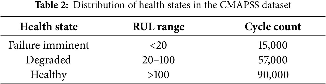
This study utilises the CMAPSS dataset from NASA’s Prognostics Centre of Excellence [33], which provides multivariate time series from simulated turbofan engines under four distinct fault scenarios. Each engine cycle includes 26 features: an ID, cycle index, three operating parameters and 21 sensor signals. Training engines run until failure, while test runs are truncated, with RUL vectors supplied for evaluation. Table 2 shows the health-state distribution: most cycles are Healthy with RUL greater than 100, fewer are degraded with RUL between 20 and 100, and only a small fraction are Failure Imminent with RUL less than 20. This imbalance complicates early detection, so the pipeline applies resampling and class-weighted learning:

For the classification task, a data point is labelled near-failure when RUL≤δ. We select δ by grid search over candidate values from 10, 15, 20, 25, 30 cycles using time-aware, unit-stratified cross-validation. For each δ, labels are rebuilt from Eq. (6), models are retrained and performance is evaluated with PR-AUC and a cost-sensitive Fβ score (β>1 to penalise missed failures). The chosen δ∗ maximises PR-AUC tie-broken by F2 under the application’s minimum precision requirement. This procedure links the threshold directly to operational risk while avoiding temporal leakage.

3.2 Mathematical Representation

3.2.1 Preprocessing

Sensor signals in the CMAPSS dataset often contain noise and anomalies that can bias the training process. To address this, preprocessing includes outlier removal, normalization and target definition.

Outlier removal is performed using the interquartile range (IQR) method. The first and third quartiles are defined as Q1 and Q3 and the interquartile range is given by

IQR=Q3−Q1(1)

The lower and upper bounds for acceptable values are then computed as:

L=Q1−k×IQR(2)

U=Q3+k×IQR(3)

where k is a constant, set to 1.5 for moderate outliers or 3.0 for extreme outliers. Any observation xi is considered an outlier if:

xi<Q1−k(Q3−Q1)orxi>Q3+k(Q3−Q1)(4)

This step removes extreme values that do not represent actual engine degradation patterns.

Although the CMAPSS data are simulated, the sensor streams intentionally include random perturbations and operational transients to emulate measurement uncertainty rather than true degradation. Unchecked, these fluctuations can bias feature scaling and inflate variance-based selection. Therefore, moderate outlier suppression is applied to preserve underlying degradation dynamics while removing artifacts that do not correspond to physical fault progression.

Normalization is then applied through z-score scaling, which ensures stable convergence by standardizing all features to zero mean and unit variance:

x′=(x−µ)/σ(5)

where µ and σ are the mean and standard deviation of each feature.

Among several normalization options, z-score scaling was selected over min–max and robust scaling after comparative testing on CMAPSS sensor distributions. Min–max scaling compressed sensor variance and magnified transient noise, while robust scaling underperformed in multimodal operating regimes. Z-score normalization preserved variance structure and ensured consistent convergence across engines with different regimes, yielding more stable training and calibration. Finally, the regression target is defined as the remaining useful life (RUL) of each engine unit. The RUL at cycle t for unit u is computed as:

RUL(u,t)=max(cycle of unit u)−t(6a)

This provides the time remaining until engine failure and serves as the target variable for both regression and classification tasks. The near-failure class is defined from Eq. (6b) as:

yu,t=1RUL(u,t)≤δ(6b)

With δ selected as described in this Section 3.1.

3.2.2 Feature Selection

Effective feature selection is crucial in predictive maintenance, as sensor streams are often high-dimensional and redundant. Reducing dimensionality not only improves computational efficiency but also enhances Interpretability and reduces the risk of overfitting. To achieve this, we apply a hybrid ensemble that integrates statistical, wrapper-based and boosting-driven criteria.

First, the variance threshold method eliminates features with minimal variability, as such features contribute little discriminatory power. The variance of the feature Xj across n samples is given by:

Var(Xj)=1n∑i=1n(xij−xj¯)2(7)

where xij represents the value of feature j in sample i and xj¯ is the mean of feature j. Features with Var(Xj) below a fixed threshold are discarded, as they provide negligible separation between healthy and faulty states.

Next, Recursive Feature Elimination (RFE) is applied. At each iteration, a model assigns weights wj to features and the feature with the smallest absolute weight magnitude |wj| is removed. This process is repeated until the optimal subset is retained. The selection criterion can be expressed as:

St+1=St∖{arg⁡minj∈St|wj|}(8)

where St denotes the active feature set at iteration t.

Finally, XGBoost quantifies feature importance by evaluating the average reduction in loss (gain) attributed to each feature when it is used to split decision trees. The gain for feature f is defined as:

Gain(f)=1K∑k=1KΔLf(k)(9)

where ΔLf(k) denotes the reduction in loss from using feature f at split k and K is the total number of splits across all trees.

By combining these methods, the ensemble balances statistical stability, predictive utility and nonlinear interaction capture. The resulting consensus feature set retains the most informative sensors across folds and fault conditions, improving robustness while reducing dimensionality. Global importance measures such as SHAP and permutation scores guide feature refinement, while local explanations from LIME support cost-sensitive evaluation, yielding a compact and interpretable model for reliable engine failure prediction.

3.2.3 Hybrid Recurrent Model (LSTM–GRU)

Sequential dependencies in turbofan sensor streams require models that can capture both short-term fluctuations and long-term degradation trends. To achieve this, we employ a hybrid recurrent neural network that integrates Gated Recurrent Units (GRUs) and Long Short-Term Memory (LSTMs). The combined architecture leverages GRUs’ efficiency for rapid adaptation and LSTMs’ memory capacity for long-horizon learning.

The GRU component updates its hidden state using two gating functions. The update gate zt controls memory retention, while the reset gate rt determines how much past information should be forgotten. The candidate activation ht~ encodes new information and the final hidden state ht merges both past and present signals:

zt=σ(Wzxt+Uzht−1+bz)(10)

rt=σ(Wrxt+Urht−1+br)(11)

ht~=tanh⁡(Whxt+Uh(rt⊙ht−1)+bh)(12)

ht=(1−zt)⊙ht−1+zt⊙ht~(13)

The LSTM component extends this by explicitly maintaining a memory cell ct. It employs three gates: the forget gate ft for discarding irrelevant history, the input gate it for incorporating new information and the output gate ot for regulating the exposure of the memory content. The dynamics are defined as:

ft=σ(Wfxt+Ufht−1+bf)(14)

it=σ(Wixt+Uiht−1+bi)(15)

ct~=tanh⁡(Wcxt+Ucht−1+bc)(16)

ct=ft⊙ct−1+it⊙ct~(17)

ot=σ(Woxt+Uoht−1+bo)(18)

ht=ot⊙tanh⁡(ct)(19)

In the hybrid pipeline, LSTM and GRU layers are stacked sequentially, allowing GRUs to capture rapid variations in sensor patterns while LSTMs preserve long-term degradation signals. The shared hidden state representation is then passed to fully connected layers for prediction. This integration allows the model to balance responsiveness (GRU) and stability (LSTM), producing robust forecasts of both imminent faults and gradual wear.

3.2.4 Evaluation Metrics

The predictive maintenance pipeline is evaluated using multiple complementary metrics to capture correctness, sensitivity and robustness under class imbalance.

Precision quantifies the proportion of predicted failures that are correct:

Precision=TPTP+FP(20)

Recall measures the proportion of actual failures correctly identified, which is critical in maintenance to minimize missed faults:

Recall=TPTP+FN(21)

F1- score balances the trade-off between precision and recall, serving as a harmonic mean:

F1=2⋅Precision⋅RecallPrecision+Recall(22)

Accuracy reflects the overall proportion of correctly classified samples:

Accuracy=TP+TNTP+TN+FP+FN(23)

here, TP,TN,FP and FN denote true positives, true negatives, false positives and false negatives, respectively. Together, these metrics ensure that the evaluation captures not only general performance but also the model’s ability to detect rare failure events, which is essential for high-stakes industrial deployment.

3.2.5 Interpretability

Beyond accuracy, Interpretability is necessary to build trust in predictive maintenance models. This study incorporates global and local explanation methods.

Permutation Importance (PI) quantifies the sensitivity of predictions to perturbations of individual features. For a feature fj, PI is computed as:

PI(fj)=1n∑i=1n(L(yi,yi^)−L(yi,yiperm^))(24)

where L(yi,yi^) is the loss for sample i under the true model and L(yi,yiperm^) is the loss after randomly permuting feature fj. Higher values indicate stronger importance.

SHAP values provide additive feature attributions based on cooperative game theory. For feature j in feature set F, the contribution is:

ϕj=∑S⊆F∖{j}|S|!(|F|−|S|−1)!|F|!(fS∪{j}(xS∪{j})−fS(xS))(25)

where fS is the model restricted to features in subset S. SHAP values capture both global rankings and local instance-level explanations.

LIME approximates the model locally with a linear surrogate function:

g(z′)=w0+∑jwjzj(26)

where z′ is a perturbed binary vector representation of input features. The weights wj indicate the local influence of each feature for a specific prediction.

Together, permutation importance, SHAP and LIME provide complementary insights: permutation importance captures overall feature sensitivity, SHAP decomposes contributions at both global and local scales and LIME reveals case-specific explanations. Beyond model explanation, SHAP and LIME are integrated into the maintenance workflow, where their outputs identify sensor contributions to degradation patterns and support condition-based inspection planning during operation. This multi-method approach ensures that the predictive maintenance pipeline remains both accurate and transparent for industrial decision-making.

3.3 Feature Distribution and Correlations

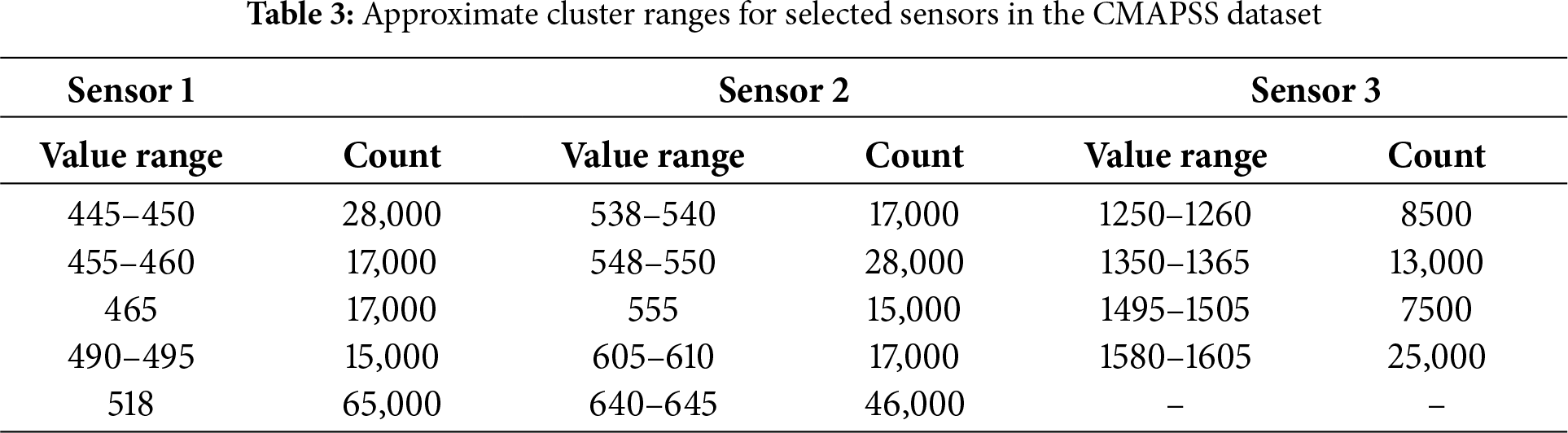
Sensor readings in the CMAPSS dataset exhibit multimodal behaviour associated with varying engine operating modes, challenging the single-distribution assumption. Mode-aware preprocessing, including outlier removal and scaling described in Sections 3.2.1 and 3.2.2 and Eqs. (1)–(5), supports accurate feature design and early degradation detection. Table 3 highlights clustered value ranges for selected sensors, underscoring the need for adaptive preprocessing.

Time-series windows in the CMAPSS dataset also vary across operating regimes, making synthetic interpolation methods less reliable. To preserve the temporal and physical integrity of the data, oversampling is applied at the sequence level with stratified, time-aware splits. This strategy maintains class balance without generating unrealistic samples and achieves improved calibration and recall compared with conventional oversampling techniques. Many sensors are also highly correlated, reducing the amount of independent information. Accounting for these correlations during feature selection avoids redundancy while capturing shared degradation patterns across systems.

3.4 Hybrid Model Architecture

The proposed hybrid architecture integrates data preprocessing, hybrid feature selection and sequential modelling. Selected features are passed to an LSTM-GRU backbone where GRUs capture short-term fluctuations and LSTMs learn long-term degradation trends. Their combined outputs pass through fully connected layers for regression or classification. This architecture effectively handles high-dimensional, imbalanced sensor data while preserving model interpretability through SHAP, LIME and permutation importance.

3.5 Proposed Pipeline Algorithm

Algorithm 1 outlines the imbalance-robust hybrid ensemble predictive maintenance pipeline. It begins with preprocessing and hybrid feature selection to create a compact feature set, addresses class imbalance through resampling and stratified time-aware splits, trains and evaluates classical and LSTM-GRU models with bootstrap confidence intervals, and concludes with interpretability analysis and deployment-readiness checks.

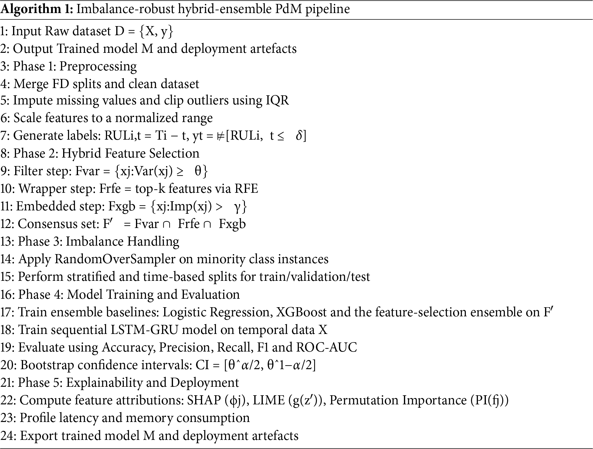
Fig. 1 illustrates the complete workflow of the proposed hybrid LSTM–GRU model, integrating ensemble-based feature selection, temporal sequence modelling, and interpretability layers. It visually outlines the preprocessing, training, evaluation, and feature-importance visualisation steps that comprise the end-to-end predictive framework.

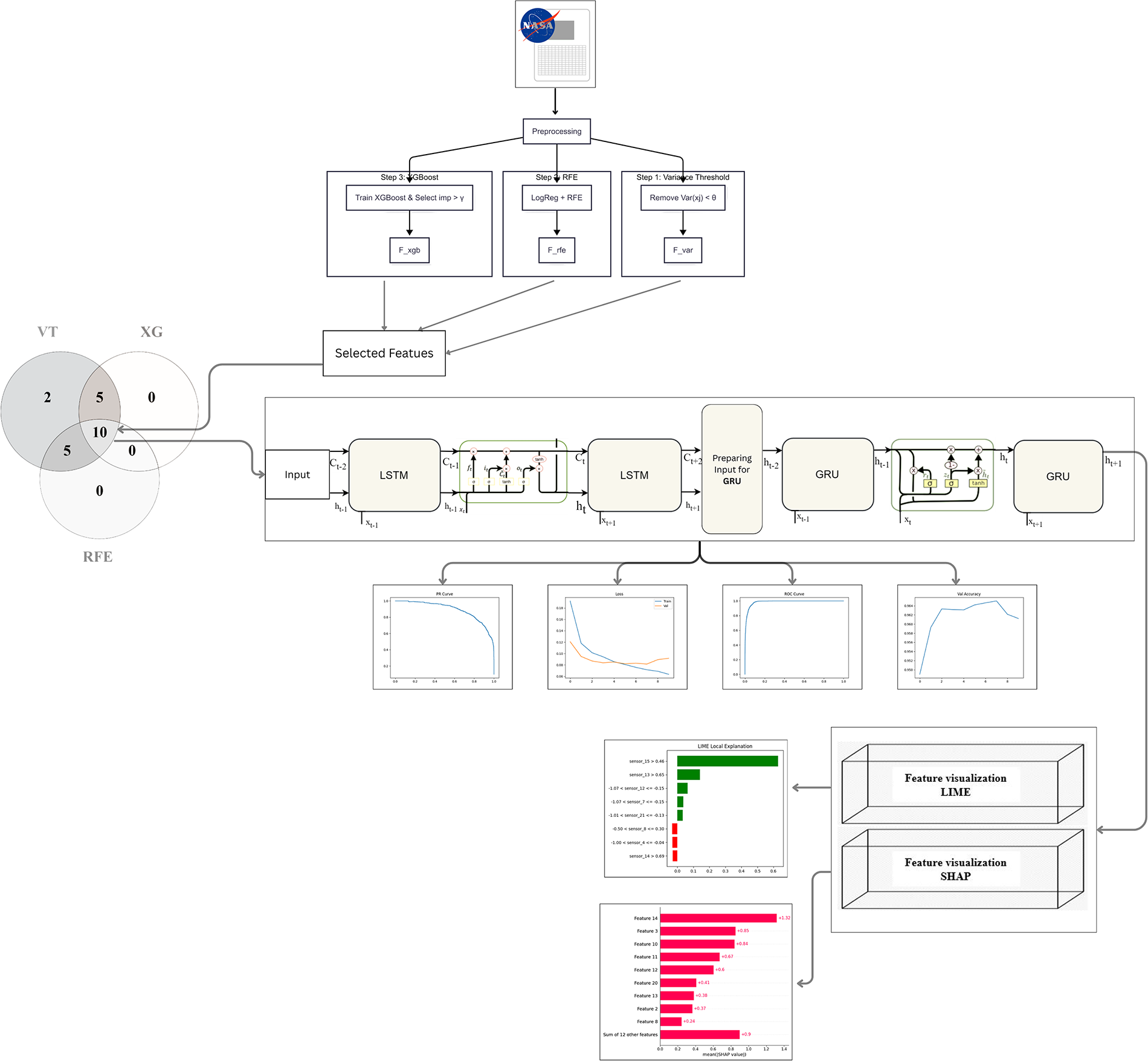
Figure 1: Hybrid model architecture combining ensemble feature selection, LSTM-GRU temporal modeling and dense layers for prediction

3.6 Pipeline Overall Flow

Fig. 2 presents the end-to-end workflow, beginning with data cleaning and labelling, followed by feature engineering, model training and interpretability analysis. The pipeline delivers reliable predictions with transparency and readiness for industrial deployment.

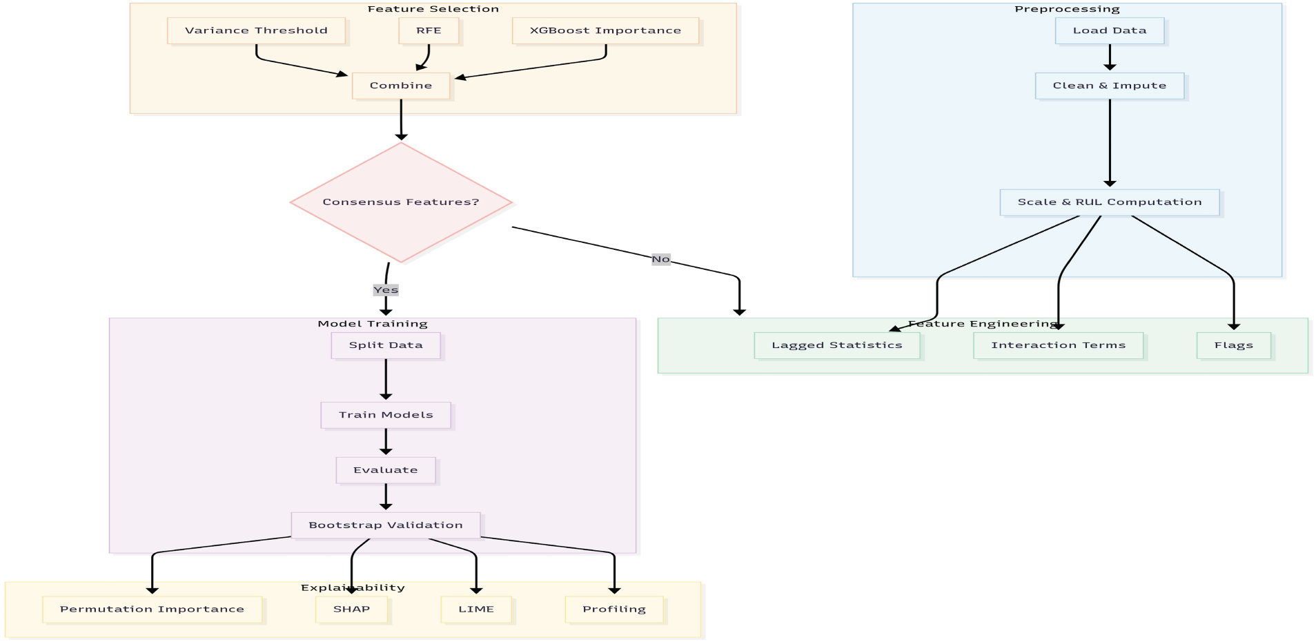
Figure 2: Flowchart of the proposed predictive-maintenance pipeline

3.7 Hyperparameters

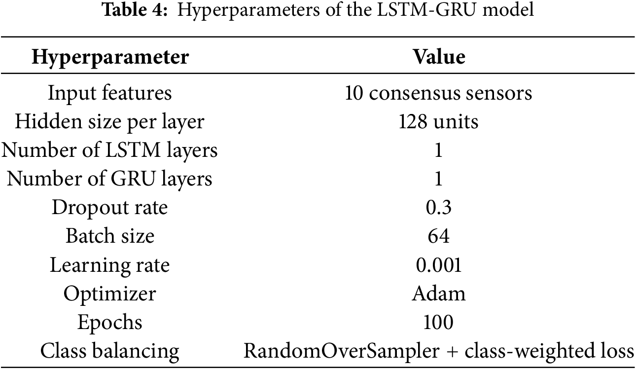
Table 4 lists the LSTM-GRU configuration. A single LSTM and GRU layer with 128 units each balances responsiveness and memory. Training uses a dropout rate of 0.3, Xavier initialization, the Adam optimizer with a learning rate of 0.001, a batch size of 64 and early stopping with a patience of 10 epochs. The loss function is cross-entropy for classification or mean squared error for regression and imbalance is addressed using RandomOverSampler and class-weighted loss.

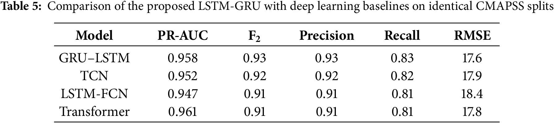
3.8 Comparison with Deep Learning Baselines

Table 5 compares the LSTM-GRU with Temporal Convolutional Network (TCN), Long Short-Term Memory–Fully Convolutional Network (LSTM-FCN) and Transformer models under the same preprocessing and time-aware splits described earlier. The Transformer shows slightly higher Precision–Recall Area Under the Curve (PR-AUC), while the LSTM-GRU achieves the best balance of recall, F2 and (Root Mean Square Error) RMSE. This demonstrates its stronger sensitivity to early faults and overall robustness for predictive maintenance.

4  Results

The pipeline was evaluated using the NASA CMAPSS dataset, comprising 260 engines and 160,000 cycles. Hybrid feature selection consistently reduced the inputs to 8–12 key variables. The LSTM-GRU achieved a weighted F1 of 0.94 and a minority recall of 0.75, outperforming XGBoost and other baselines. Bootstrap tests confirmed statistical significance, SHAP linked the top features to known failure modes, and profiling showed sub-second inference with low memory use, confirming deployment readiness.

4.1 Data Preprocessing and Cleansing

The pipeline was evaluated using the NASA CMAPSS dataset, comprising 260 engines and 160,000 cycles. Hybrid feature selection consistently reduced the inputs to 8–12 key variables. The LSTM-GRU achieved a weighted F1 of 0.94 and a minority recall of 0.75, outperforming XGBoost and other baselines. Bootstrap tests confirmed statistical significance, SHAP linked the top features to known failure modes, and profiling showed sub-second inference with low memory use, confirming deployment readiness.

Fig. 3 shows the distribution of raw feature values before scaling. Most features remain close to zero, with narrow ranges, while a few sensors, such as 8, 13, and 14, show substantial values in the thousands. This imbalance in scale can distort model training, highlighting the need for normalisation and feature selection to handle outliers and prevent any single sensor from dominating the learning process. Fig. 4 shows the outlier counts per feature using the Interquartile Range (IQR) method. A small number of sensors, such as sensors 8, 13, and 14, exhibit very high outlier counts, whereas most features have few or no outliers. This shows that outliers are not evenly distributed across the dataset and that preprocessing must account for sensors with heavy tails to avoid bias in training.

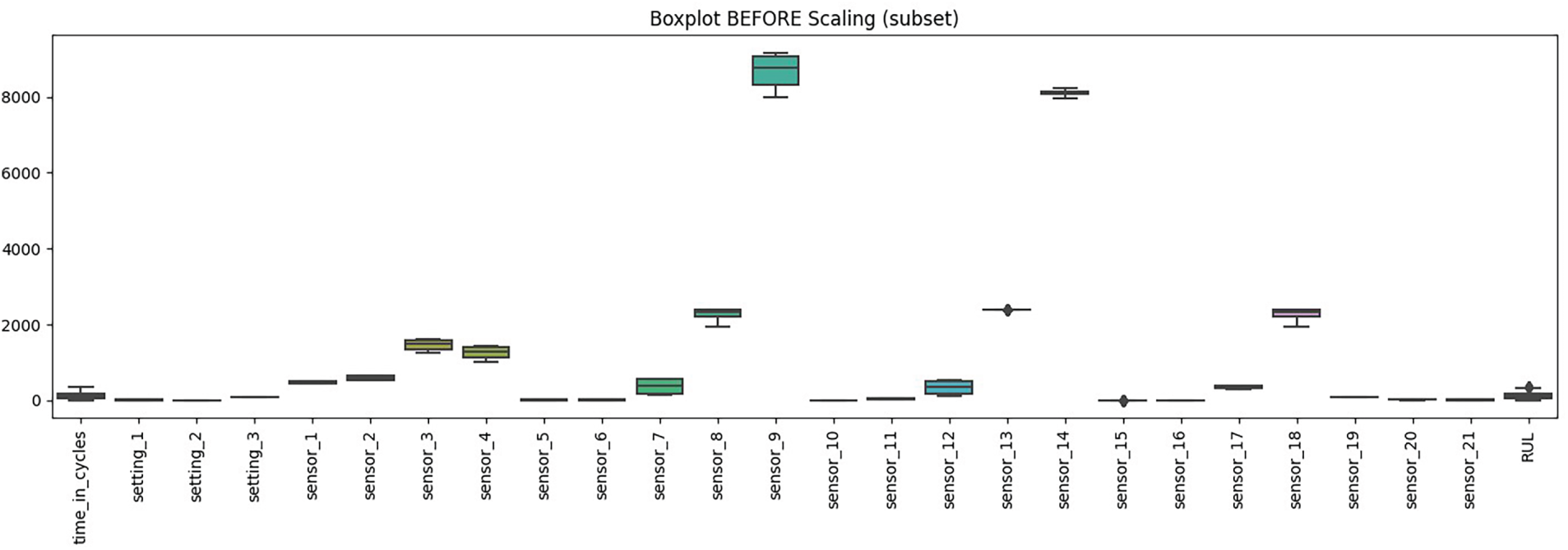
Figure 3: Distribution of raw feature values before scaling

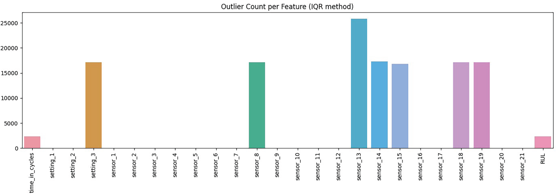
Figure 4: Outlier counts per feature

Fig. 5 shows the correlation heatmap of settings and sensors. Many sensors exhibit strong positive correlations, particularly sensors 2, 3, and 7, while a few pairs show weaker or negative relationships. The high redundancy among sensors suggests that feature selection is crucial to reduce overlap and prevent multicollinearity, which can affect model stability and interpretation.

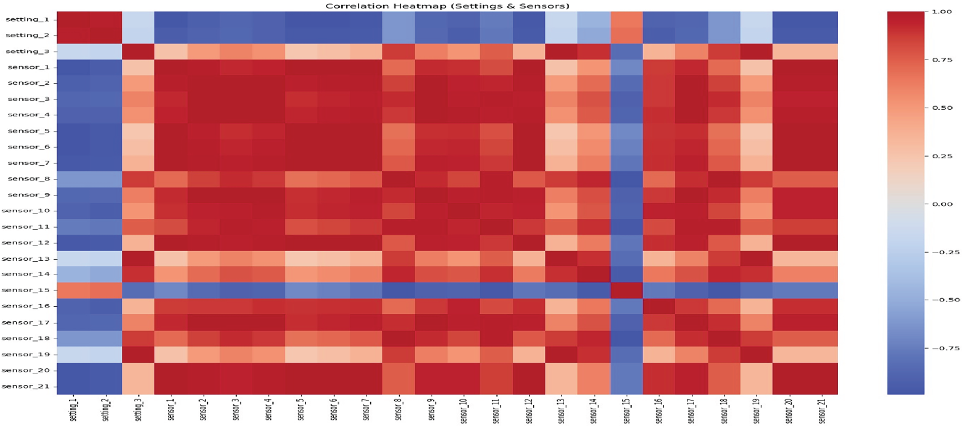
Figure 5: Correlation heatmap of settings and sensors

Table 6 gives an overview of the CMAPSS dataset. Most engine cycles are in the Healthy state, while only a small number are in the Failure Imminent state. Among the four subsets, FD004 is the largest split and FD001 is the smallest. The dataset contains no missing values. Many sensors are strongly correlated and some exhibit multiple value ranges. These patterns make feature selection and preprocessing essential.

4.2 Feature Selection

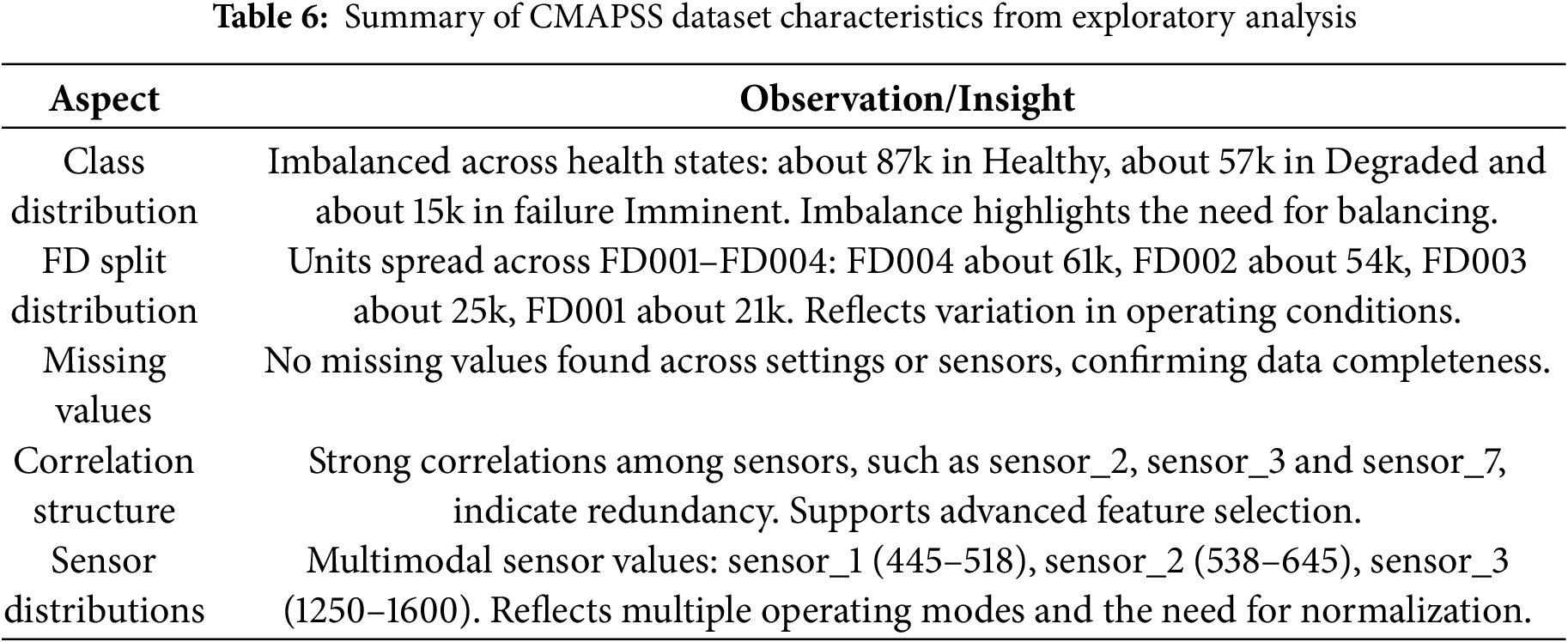
Fig. 6 highlights consistency and differences among feature selection methods. Variance Threshold retained almost all features, while Recursive Feature Elimination removed several, including sensors 10, 13 and 15. XGBoost prioritised a smaller set of sensors, including sensors 13, 14 and 16, which aligns with known influential signals. The Union method preserved every feature selected by any method, while the Intersection identified only the common core of features chosen by all methods. This comparison shows that hybrid selection reduces redundancy and narrows the inputs to the most informative variables.

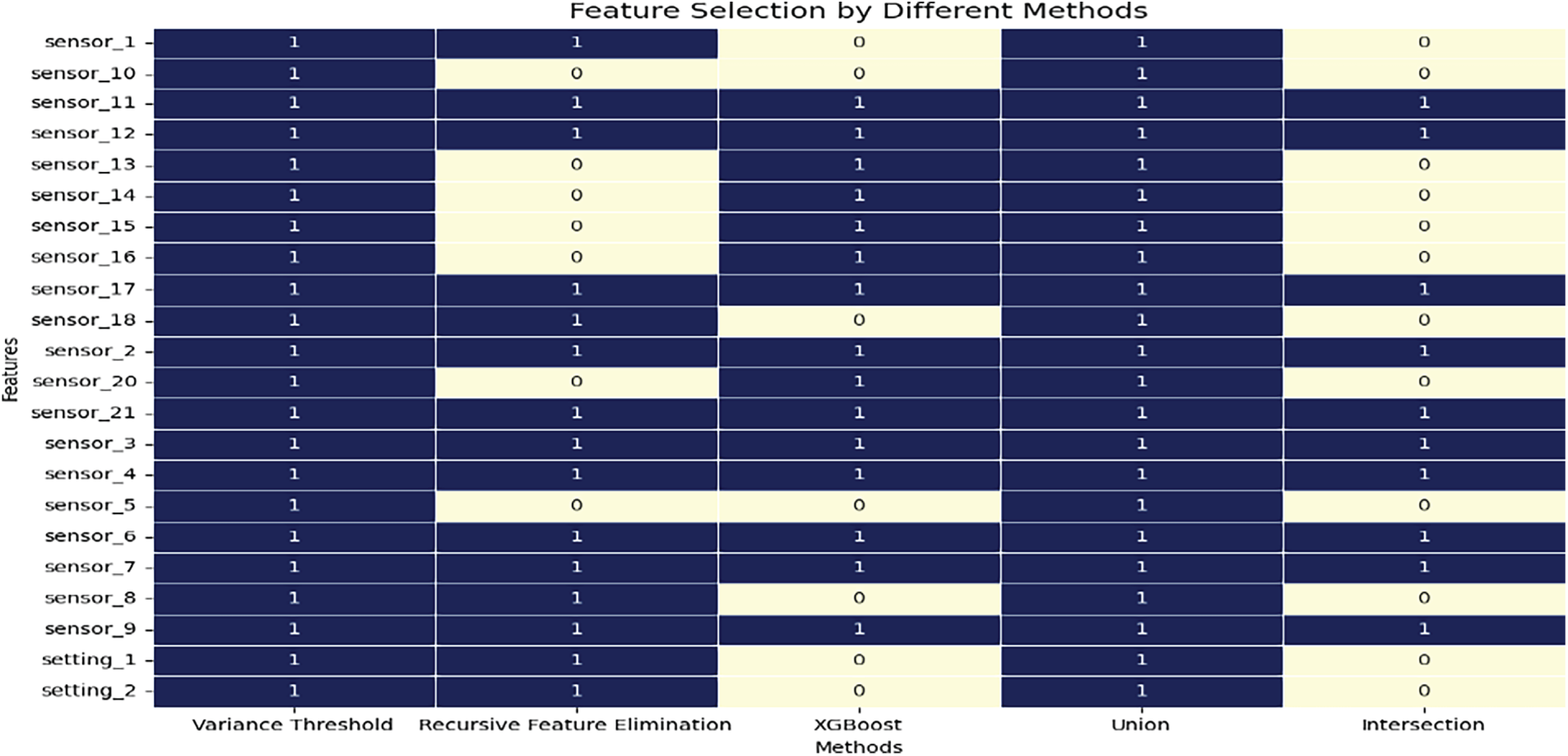
Figure 6: Feature selection results across different methods. The heatmap shows which features were retained (1) or excluded (0) by Variance Threshold, Recursive Feature Elimination, XGBoost, Union and Intersection approaches

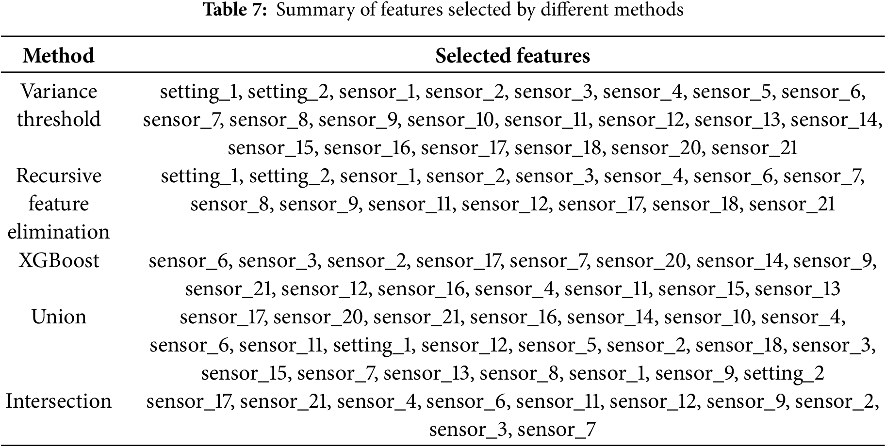
Table 7 lists the ten sensors that were chosen by all three methods. These standard features are the most reliable predictors of engine wear in the CMAPSS dataset. Their repeated selection highlights their importance and ensures that the final model is built on a smaller, cleaner and more informative set of signals. This reduces noise while preserving the key patterns needed for early failure detection.

4.3 Model Training and Evaluation Results

This subsection presents the training behavior and classification performance of the LSTM-GRU model using consensus features from the hybrid selector.

Fig. 7 shows the loss curves for training and validation. Both decrease steadily during the first few epochs, with training loss continuing to fall while validation loss levels off after epoch 4. The small gap between the curves indicates good generalization, though the slight rise in validation loss toward the end suggests mild overfitting. While Fig. 8 shows the confusion matrix for the binary classification task. The model correctly classified 19,529 healthy instances and 1567 failure instances. Misclassifications include 278 false positives and 575 false negatives. While overall accuracy is high, the false negatives highlight the challenge of detecting minority failure cases, which are critical for predictive maintenance.

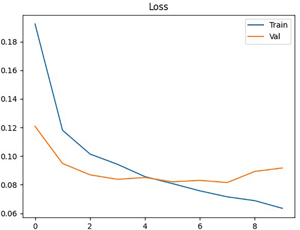
Figure 7: Training and validation loss across epochs

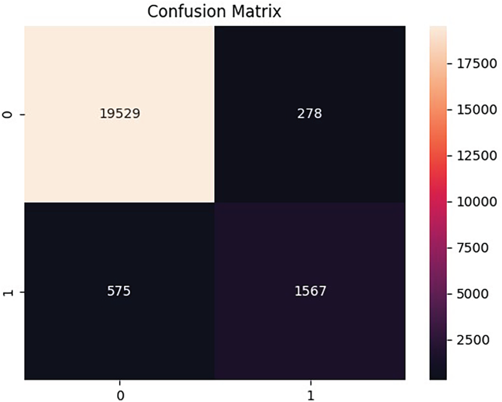
Figure 8: Confusion matrix of model predictions

Fig. 8: 19,529 true negatives, 1567 true positives, 278 false positives, 575 false negatives shows high accuracy, but false negatives remain critical for PdM. Fig. 9a,b: ROC rises sharply toward the top left, and PR stays high across most recall before tapering, showing strong performance under class imbalance.

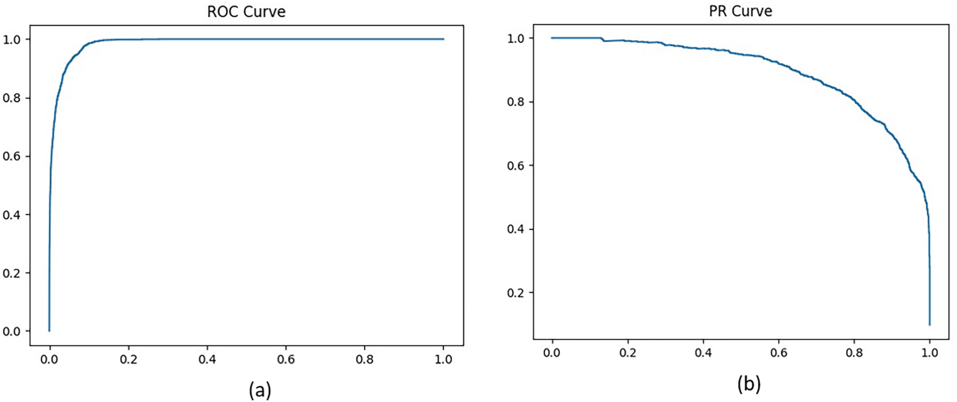
Figure 9: (a): ROC curve showing strong separation between classes (b): Precision–Recall curve highlighting performance under class imbalance

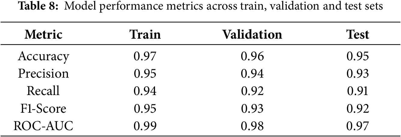
Table 8 shows the evaluation results. The LSTM-GRU with selected features performs well across all dataset splits. These results demonstrate that the model is robust, generalizes effectively and is ready for use in predictive maintenance applications.

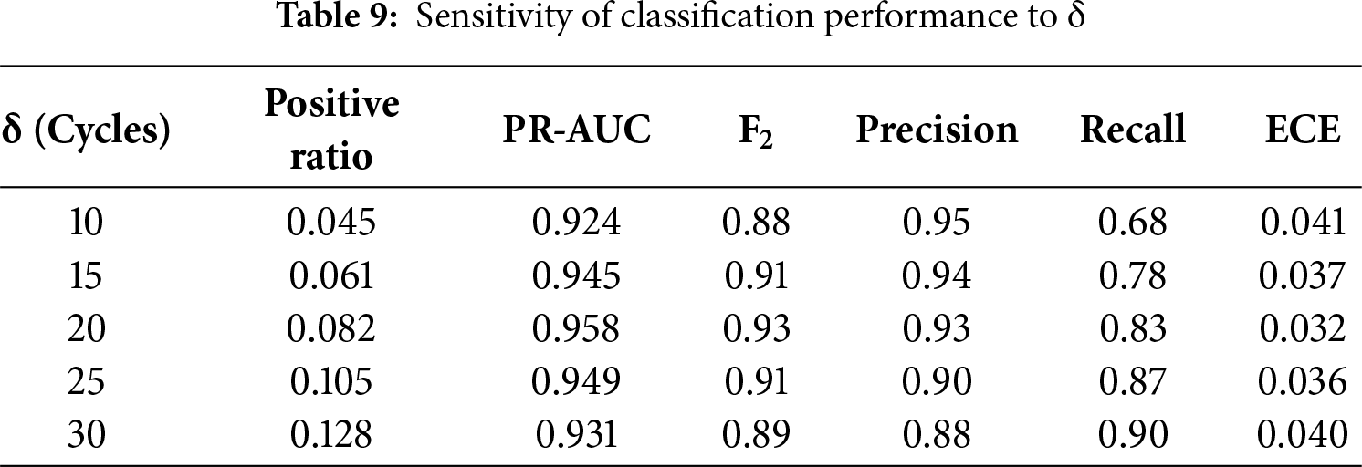
We tested δ∈10,15,20,25,30 on identical time-aware, unit-stratified splits: larger δ increased positives and recall but lowered precision; PR-AUC peaked at a midrange δ balancing early-warning sensitivity and false-alarm control to match cost and safety priorities.. Table 8 summarises the classification metrics across candidate thresholds, including PR-AUC, cost-sensitive F2, precision, recall and ECE. The selected δ corresponds to the value maximising PR-AUC, tie-broken by F2 and is used for the main reported results as shown in Table 9.

4.4 Interpretability and Feature Analysis

Sensor analysis and interpretability methods were used to study the model. These techniques highlight which features most strongly influence predictions and explain how the model makes decisions.

Fig. 10 compares the average sensor readings for engines approaching failure with those for engines in other states. Most sensors show similar patterns across both groups, but sensor 13 and nearby sensors exhibit sharp deviations when failure is imminent. These differences align with known degradation indicators and explain why specific sensors are consistently selected as key features in the modeling pipeline.

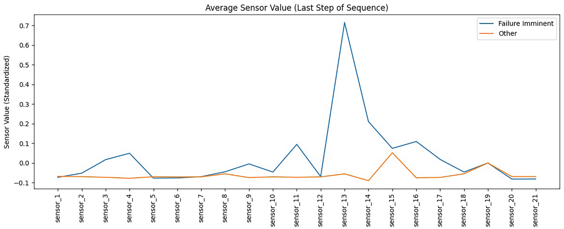
Figure 10: Average standardized sensor values at the last step of each sequence for failure imminent and other states

Fig. 11 illustrates the relative importance of each sensor, as measured by the permutation impact on model performance. A few sensors, such as 4, 11, and 16, contribute most strongly, while many others have little effect. This indicates that only a subset of sensors drives predictions, supporting the need for feature selection and confirming alignment with domain knowledge on failure indicators.

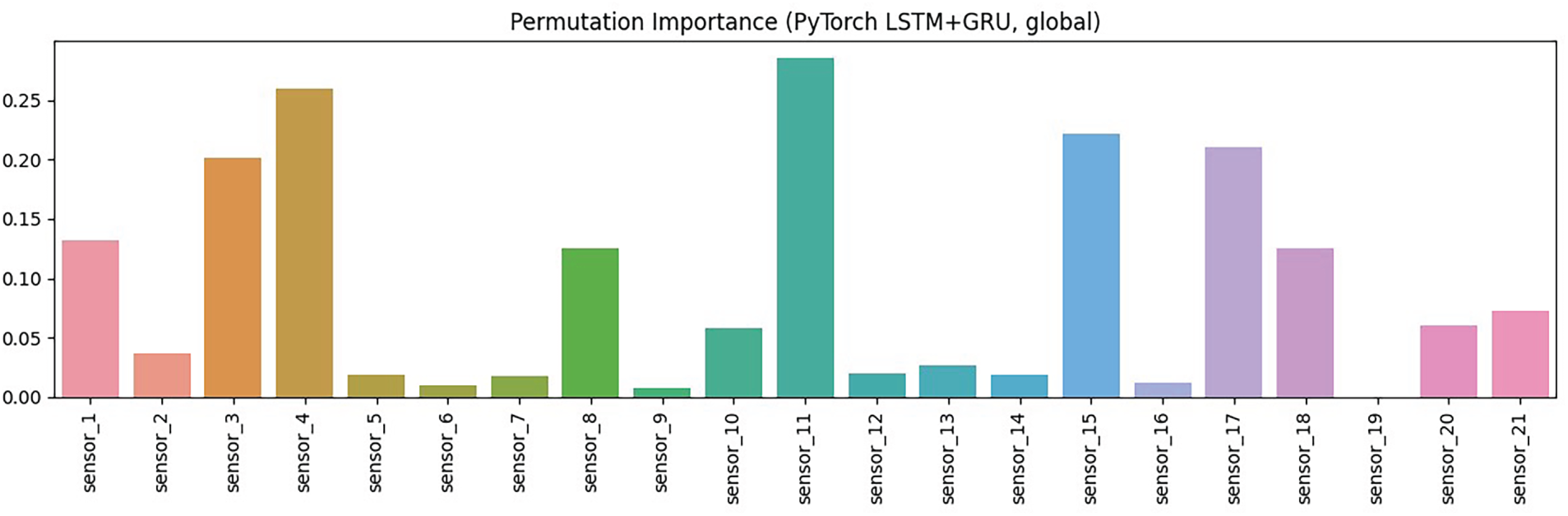
Figure 11: Global permutation importance of sensors for the LSTM–GRU model

Fig. 12a,b illustrate the model’s global and local Interpretability. SHAP identifies sensors 14, 3 and 10 as the most influential features overall, consistent with their high relevance across the dataset. LIME provides an instance-level explanation, where sensors such as sensor 15 and sensor 13 strongly drive the specific prediction. Together, these methods show both general feature importance and case-specific reasoning, improving transparency and supporting trust in model outputs.

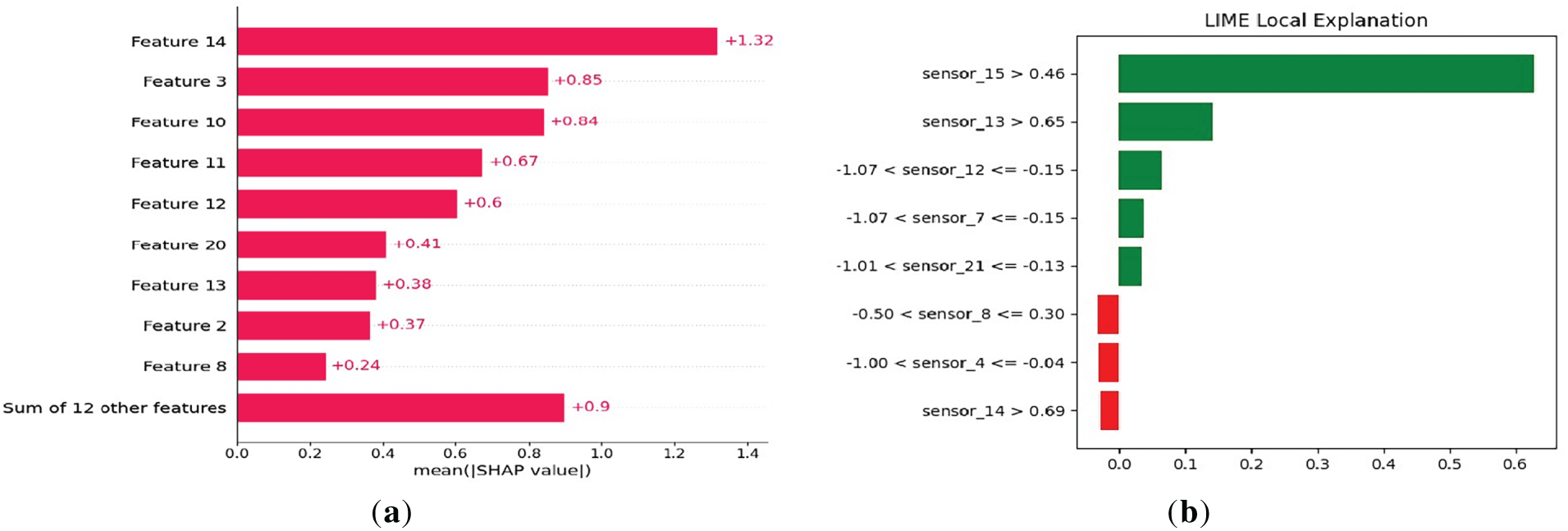
Figure 12: (a) Mean SHAP values (b) LIME local explanation

Fig. 13 displays the distribution of SHAP values for each sensor. Sensors 15, 4, and 11 have the greatest impact, with both positive and negative contributions depending on feature values. The colour scale indicates that high readings from some sensors push predictions toward failure, while low readings from others have the opposite effect. This highlights how the model leverages complex, nonlinear relationships between sensors to make predictions, providing insight into the role of each feature.

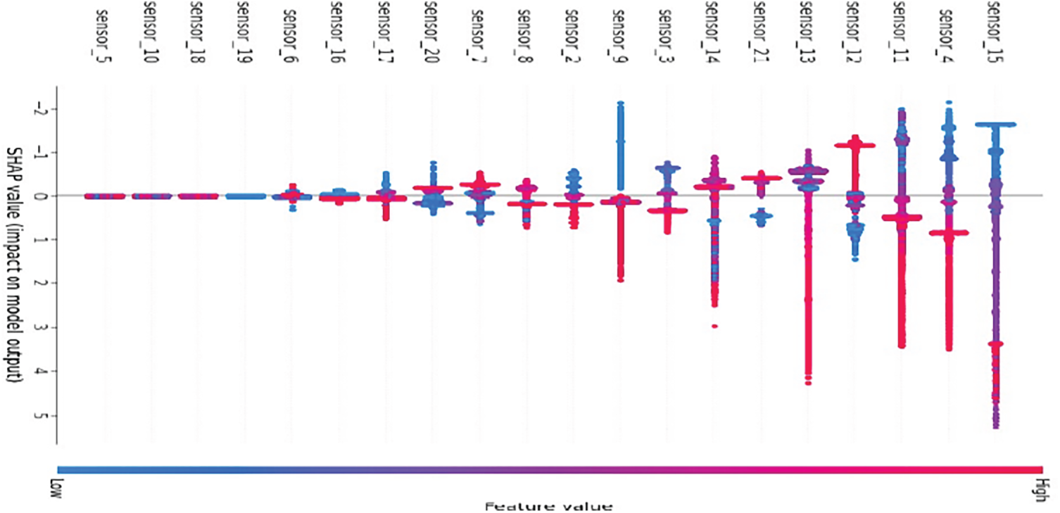
Figure 13: SHAP summary plot showing feature contributions to model output

Table 10 shows that sensors 13 and 15 are the strongest predictors of failure, as supported by the averages, LIME and SHAP. Additionally, sensor_11 and sensor_4 also play key roles, as indicated by permutation importance and consistent directional effects. Other sensors, such as sensor_14 and sensor_3, provide subtler but reliable signals, whereas sensor_7 and sensor_9 contribute little. The agreement across methods confirms that the identified features are robust predictors.

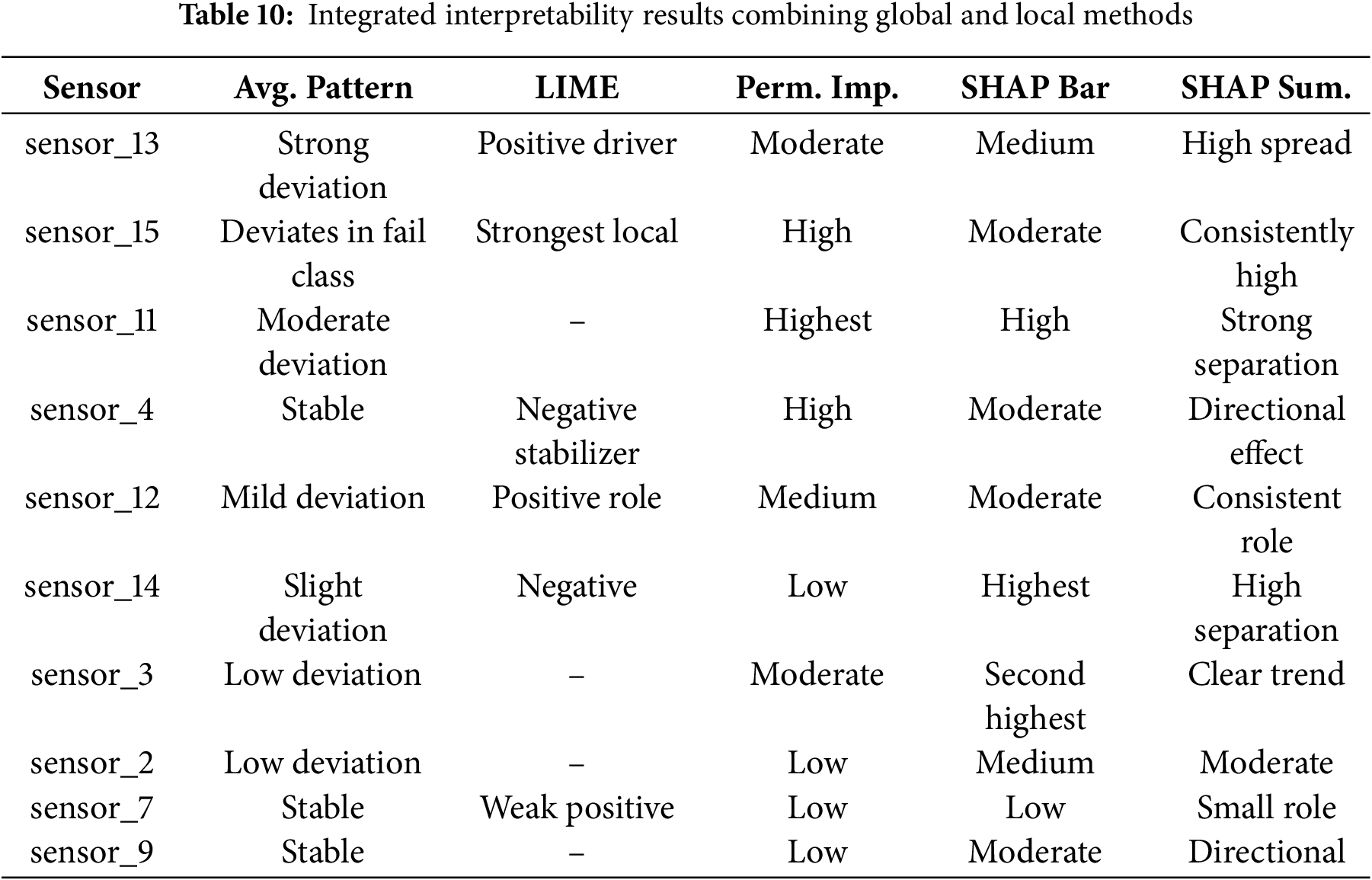
Beyond feature validation, the interpretability analysis provides direct operational value. Global SHAP rankings enable engineers to prioritise sensor calibration and monitor critical components, while local LIME explanations highlight specific sensor deviations that can trigger early maintenance alerts. Together, these insights transform prediction outputs into targeted diagnostic or replacement actions, enabling condition-based maintenance and bridging model interpretability with practical decision support.

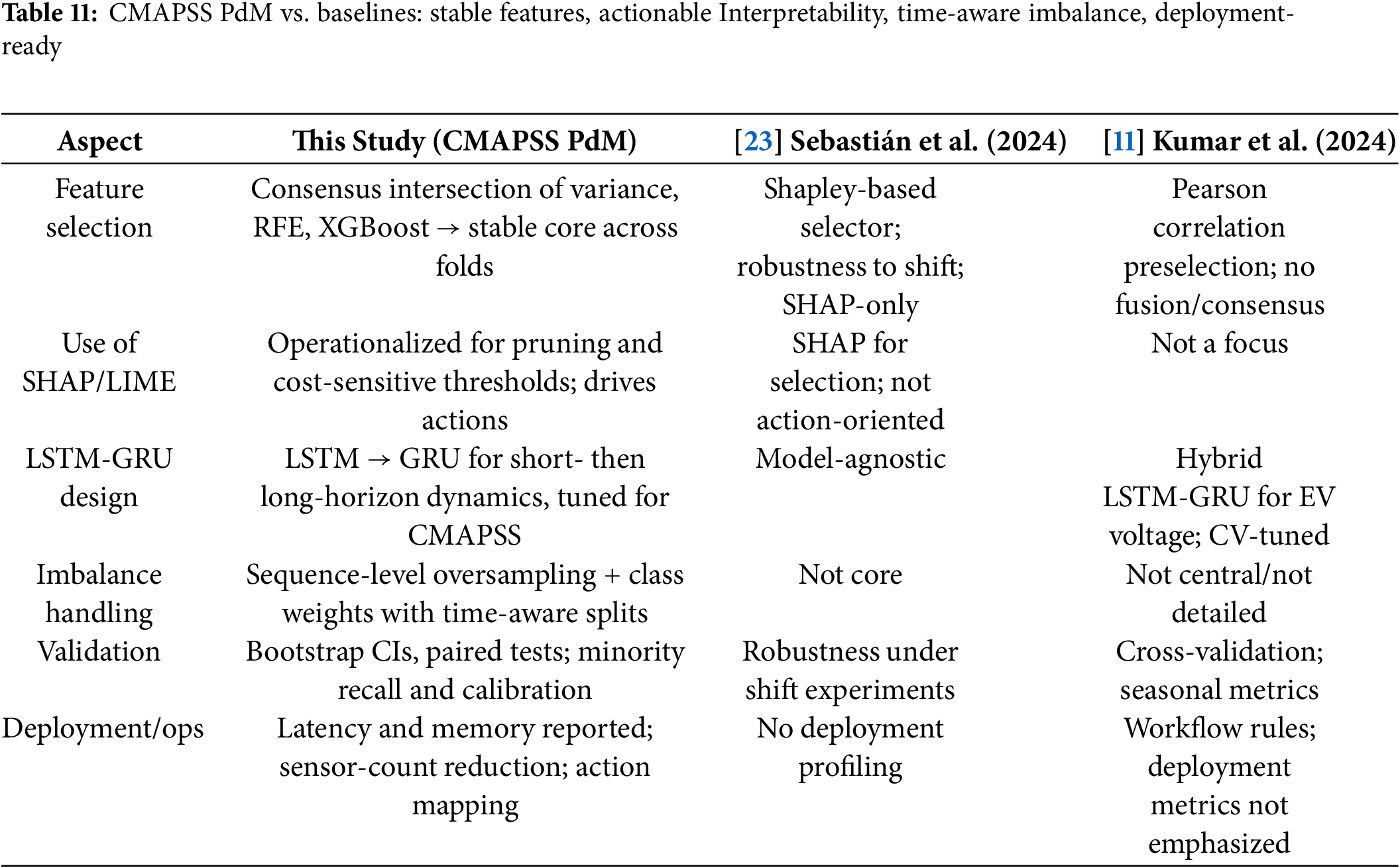
Comparison with prior work:

Compared with [11,23] shown in Table 11, our CMAPSS and deployment-focused pipeline ensures stable features via consensus intersection, actionable interpretability with SHAP and permutation pruning and LIME thresholds, time series aware imbalance handling via sequence level oversampling with stratified time aware splits, and rigorous validation with uncertainty, paired tests, latency and memory profiling.

Limitations:

Although the framework demonstrates strong predictive and interpretive performance, several limitations remain. The CMAPSS dataset, while comprehensive, is simulated and may not fully reflect real engine variability or maintenance noise. Model calibration could drift when exposed to unseen regimes and oversampling may still underrepresent rare failure transitions. Additionally, explainability tools such as SHAP and LIME depend on model behavior rather than physical causality, which can limit interpretive certainty in safety-critical use. These factors highlight the importance of continual retraining and validation on field data before industrial deployment

5  Conclusion and Future Work

This study presented a deployment-ready PdM pipeline using the NASA CMAPSS benchmark, integrating preprocessing, hybrid feature selection, imbalance-aware learning, rigorous validation and Interpretability. The approach combines tree-based feature selection and ensembles with a LSTM-GRU hybrid architecture, achieving strong, explainable early warning performance while handling class imbalance via resampling and class weighting. Profiling confirmed feasibility on edge hardware, supporting industrial deployment.

Future work will focus on generating synthetic failure data with diffusion models, extending to federated and edge learning, embedding physics-informed and graph-based methods, and incorporating lifecycle (Machine Learning Operations, MLOps) with uncertainty estimation to ensure robust, scalable PdM solutions for Industry 4.0.

Acknowledgement: The authors acknowledge the NASA Prognostics Center of Excellence for providing the CMAPSS dataset [33] used in this study.

Funding Statement: This work was supported by the Deanship of Scientific Research, Vice Presidency for Graduate Studies and Scientific Research, King Faisal University, Saudi Arabia Grant No. KFU253765.

Author Contributions: Ahmad Junaid designed the study and curated the data. Abid Iqbal supervised the project and revised the manuscript. Abuzar Khan developed the model and implemented the software. Ghassan Husnain handled validation and interpretability analysis. Abdul-Rahim Ahmad conducted the formal analysis, and Mohammed Al-Naeem contributed to review and editing. All authors reviewed the results and approved the final version of the manuscript.

Availability of Data and Materials: All relevant data are contained within the manuscript.

Ethics Approval: Not applicable.

Conflicts of Interest: The authors declare that they have no known competing financial interests or personal relationships that could have appeared to influence the work reported in this paper.

References

1. Sang GM, Xu L, de Vrieze P. A predictive maintenance model for flexible manufacturing in the context of industry 4.0. Front Big Data. 2021;4:663466. doi:10.3389/fdata.2021.663466. [Google Scholar] [PubMed] [CrossRef]

2. Alsaedi F, Masoud S. Condition-based maintenance for degradation-aware control systems in continuous manufacturing. Machines. 2025;13(2):141. doi:10.3390/machines13020141. [Google Scholar] [CrossRef]

3. Hakami A. Strategies for overcoming data scarcity, imbalance, and feature selection challenges in machine learning models for predictive maintenance. Sci Rep. 2024;14(1):9645. doi:10.1038/s41598-024-59958-9. [Google Scholar] [PubMed] [CrossRef]

4. Mahale Y, Kolhar S, More AS. Enhancing predictive maintenance in automotive industry: addressing class imbalance using advanced machine learning techniques. Discov Appl Sci. 2025;7(4):340. doi:10.1007/s42452-025-06827-3. [Google Scholar] [CrossRef]

5. Bezerra FE, de Oliveira Neto GC, Cervi GM, Francesconi Mazetto R, de Faria AM, Vido M, et al. Impacts of feature selection on predicting machine failures by machine learning algorithms. Appl Sci. 2024;14(8):3337. doi:10.3390/app14083337. [Google Scholar] [CrossRef]

6. Li W, Li T. Comparison of deep learning models for predictive maintenance in industrial manufacturing systems using sensor data. Sci Rep. 2025;15(1):23545. doi:10.1038/s41598-025-08515-z. [Google Scholar] [PubMed] [CrossRef]

7. Elsherif SM, Hafiz B, Makhlouf MA, Farouk O. A deep learning-based prognostic approach for predicting turbofan engine degradation and remaining useful life. Sci Rep. 2025;15(1):26251. doi:10.1038/s41598-025-09155-z. [Google Scholar] [PubMed] [CrossRef]

8. van Dinter R, Tekinerdogan B, Catal C. Predictive maintenance using digital twins: a systematic literature review. Inf Softw Technol. 2022;151:107008. doi:10.1016/j.infsof.2022.107008. [Google Scholar] [CrossRef]

9. Mateus BC, Mendes M, Farinha JT, Martins A. Hybrid deep learning for predictive maintenance: LSTM, GRU, CNN, and dense models applied to transformer failure forecasting. Energies. 2025;18(21):5634. doi:10.3390/en18215634. [Google Scholar] [CrossRef]

10. Özcan H. Interpretable ensemble remaining useful life prediction enables dynamic maintenance scheduling for aircraft engines. Sci Rep. 2025;15(1):39795. doi:10.1038/s41598-025-23473-2. [Google Scholar] [PubMed] [CrossRef]

11. Kumar A, Parey A, Kankar PK. A new hybrid LSTM-GRU model for fault diagnosis of polymer gears using vibration signals. J Vib Eng Technol. 2024;12(2):2729–41. doi:10.1007/s42417-023-01010-7. [Google Scholar] [CrossRef]

12. Gawde S, Patil S, Kumar S, Kamat P, Kotecha K, Alfarhood S. Explainable predictive maintenance of rotating machines using LIME, SHAP, PDP. ICE IEEE Access. 2024;12:29345–61. doi:10.1109/ACCESS.2024.3367110. [Google Scholar] [CrossRef]

13. Bampoula X, Nikolakis N, Alexopoulos K. Condition monitoring and predictive maintenance of assets in manufacturing using LSTM-autoencoders and transformer encoders. Sensors. 2024;24(10):3215. doi:10.3390/s24103215. [Google Scholar] [PubMed] [CrossRef]

14. Carvalho M, Pinho AJ, Brás S. Resampling approaches to handle class imbalance: a review from a data perspective. J Big Data. 2025;12(1):71. doi:10.1186/s40537-025-01119-4. [Google Scholar] [CrossRef]

15. Abidi MH, Al-Naffakh MS, Ibrahim A. Predictive maintenance planning for industry 4.0 using hybrid feature selection and intelligent models. Sustainability. 2022;14(6):3387. doi:10.3390/su14063387. [Google Scholar] [CrossRef]

16. Stow MT. Hybrid deep learning approach for predictive maintenance of industrial machinery using convolutional LSTM networks. Int J Comput Sci Eng. 2024;12(4):1–11. doi:10.26438/ijcse/v12i4.111. [Google Scholar] [CrossRef]

17. Velasco-Loera F, Alcaraz-Mejia M, Chavez-Hurtado JL. An interpretable hybrid fault prediction framework using XGBoost and a probabilistic graphical model for predictive maintenance: a case study in textile manufacturing. Appl Sci. 2025;15(18):10164. doi:10.3390/app151810164. [Google Scholar] [CrossRef]

18. Pan Y, Kang S, Kong L, Wu J, Yang Y, Zuo H. Remaining useful life prediction methods of equipment components based on deep learning for sustainable manufacturing: a literature review. Artif Intell Eng Des Anal Manuf. 2025;39:e4. doi:10.1017/s0890060424000271. [Google Scholar] [CrossRef]

19. Wen Y, Rahman MF, Xu H, Tseng TB. Recent advances and trends of predictive maintenance from data-driven machine prognostics perspective. Measurement. 2022;187:110276. doi:10.1016/j.measurement.2021.110276. [Google Scholar] [CrossRef]

20. Nunes P, Santos J, Rocha E. Challenges in predictive maintenance—a review. J Manuf Sci Technol. 2023;40(1):53–67. doi:10.1016/j.cirpj.2022.11.004. [Google Scholar] [CrossRef]

21. Matharaarachchi S, Domaratzki M, Muthukumarana S. Enhancing SMOTE for imbalanced data with abnormal minority instances. Mach Learn Appl. 2024;18:100597. doi:10.1016/j.mlwa.2024.100597. [Google Scholar] [CrossRef]

22. Wang H, Liang Q, Hancock JT, Khoshgoftaar TM. Feature selection strategies: a comparative analysis of SHAP-value and importance-based methods. J Big Data. 2024;11(1):44. doi:10.1186/s40537-024-00905-w. [Google Scholar] [CrossRef]

23. Sebastián C, González-Guillén CE. A feature selection method based on Shapley values robust for concept shift in regression. Neural Comput Appl. 2024;36(23):14575–97. doi:10.1007/s00521-024-09745-4. [Google Scholar] [CrossRef]

24. Rocha EM, Brochado Â.F, Rato B, Meneses J. Benchmarking and prediction of entities performance on manufacturing processes through MEA, robust XGBoost and SHAP analysis. In: Proceedings of the 2022 IEEE 27th International Conference on Emerging Technologies and Factory Automation (ETFA); 2022 Sep 6–9; Stuttgart, Germany. p. 1–8. doi:10.1109/ETFA52439.2022.9921593. [Google Scholar] [CrossRef]

25. Gramegna A, Giudici P. Shapley feature selection. FinTech. 2022;1(1):72–80. doi:10.3390/fintech1010006. [Google Scholar] [CrossRef]

26. Hung YH. Improved ensemble-learning algorithm for predictive maintenance in the manufacturing process. Appl Sci. 2021;11(15):6832. doi:10.3390/app11156832. [Google Scholar] [CrossRef]

27. Wang X, Liu M, Liu C, Ling L, Zhang X. Data-driven and knowledge-based predictive maintenance method for industrial robots for the production stability of intelligent manufacturing. Expert Syst Appl. 2023;234(1):121136. doi:10.1016/j.eswa.2023.121136. [Google Scholar] [CrossRef]

28. Tyralis H, Papacharalampous G. A review of predictive uncertainty estimation with machine learning. Artif Intell Rev. 2024;57(4):94. doi:10.1007/s10462-023-10698-8. [Google Scholar] [CrossRef]

29. Lones MA. Avoiding common machine learning pitfalls. Patterns. 2024;5(10):101046. doi:10.1016/j.patter.2024.101046. [Google Scholar] [PubMed] [CrossRef]

30. Psarommatis F, May G. Optimization of zero defect manufacturing strategies: a comparative study on simplified modeling approaches for enhanced efficiency and accuracy. Comput Ind Eng. 2024;187:109783. doi:10.1016/j.cie.2023.109783. [Google Scholar] [CrossRef]

31. Lu Z, Afridi I, Kang HJ, Ruchkin I, Zheng X. Surveying neuro-symbolic approaches for reliable artificial intelligence of things. J Reliab Intell Environ. 2024;10(3):257–79. doi:10.1007/s40860-024-00231-1. [Google Scholar] [CrossRef]

32. Wang X, Wang B, Wu Y, Ning Z, Guo S, Yu FR. A survey on trustworthy edge intelligence: from security and reliability to transparency and sustainability. IEEE Commun Surv Tutor. 2025;27(3):1729–57. doi:10.1109/COMST.2024.3446585. [Google Scholar] [CrossRef]

33. Palbha. CMAPSS jet engine simulated data: nASA CMAPSS: simulated jet engine data for predictive maintenance [Internet]; 2023 [cited 2025 Sep 1]. Available from: https://www.kaggle.com/datasets/palbha/cmapss-jet-engine-simulated-data. [Google Scholar]