Non-Euclidean Models for Fraud Detection in Irregular Temporal Data Environments

1  Introduction

Credit card transactions are on the rise, driven by the convenience of digital payment methods and the rapid growth of e-commerce. However, with the increase in credit card transactions, fraudulent activities have also become more frequent. According to the Nilson Report (January 2025), global card fraud losses reached $33.83 billion in 2023, and cumulative losses are projected to reach $403.88 billion over the next decade [1]. Fraudulent transactions cause significant economic losses to financial institutions and consumers, highlighting the critical need for reliable detection methods.

Traditional methods for detecting credit card fraud typically focus on large transactions at specific merchants during certain times. For instance, instead of looking for fraud on a per-customer basis, these methods concentrate on big purchases at major retailers or transactions involving large sums of money [2]. This approach treats each transaction separately when checking for fraud. This implies that each transaction is assessed independently for potential fraudulent activity.

In contrast, this study explores the analysis of fraudulent transactions under the assumption that transactions are not independent. By considering the dependencies among transactions, this study aims to identify fraudulent activities through their connections. This approach recognizes that fraudulent transactions often exhibit patterns and relationships that can be more effectively detected when analyzed together. This concept is illustrated in Fig. 1.

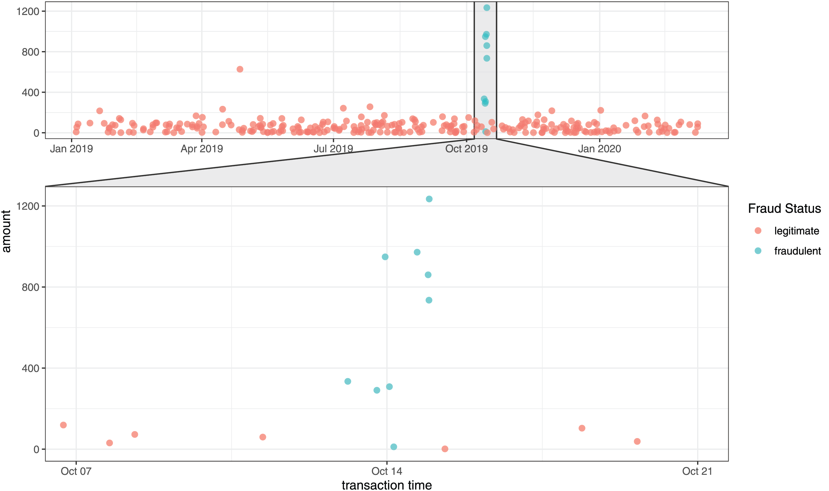
Figure 1: Transaction occurrences over time for customer Steven Johnson. Data source: Kaggle simulated credit card transaction dataset (see Section 3 for details). The x-axis represents transaction time and the y-axis represents transaction amount. Red dots indicate legitimate transactions, and blue dots indicate fraudulent transactions. The lower panel zooms into October 7–20 to highlight the temporal clustering of fraudulent transactions

Fig. 1 shows how transactions happen over time and the amounts involved in each transaction. The term ‘amount’ refers to how much money was spent in a transaction. In this figure, 12 fraudulent transactions are linked to an individual named Steven, showing that these transactions happened close to each other in time. It is clear that the amounts in these fraudulent transactions are generally higher than those in legitimate ones. When we look closely at the periods when these fraudulent transactions happened (as seen in the zoomed-in section of Fig. 1), we can see that these fraudulent transactions occurred one after another. The goal of this analysis is to use the timing of transactions to identify fraud by looking at how these fraudulent activities are connected over time.

As discussed earlier, many existing methods for detecting fraud rely heavily on the amounts of the transactions. They often identify transactions as suspicious if they involve unusually large amounts of money. Simply put, if a person who usually spends about $30 suddenly makes a $1000 transaction, it is likely to be considered fraudulent. This reliance on transaction amounts is evident when examining the distribution of transaction values in the data.

This approach may seem efficient but it is not foolproof. For example, in Fig. 1, the sixth fraudulent transaction has a very small amount, making it difficult to predict it as a fraudulent transaction. How can we identify such a transaction as fraudulent? One might think we should determine its fraudulent nature using other explanatory variables (excluding the amount), but this is often impractical with real data. This is because the sixth fraudulent transaction is very close in time to the fifth and seventh fraudulent transactions, and therefore, due to the nature of the data, other variables (such as store information or customer characteristics like age and gender) cannot show significant differences.

In fact, we can intuitively infer that the sixth transaction is fraudulent, even though it has a small amount, because all the surrounding transactions are also fraudulent. For the sixth transaction to be legitimate, it would require an unlikely scenario where a user loses their credit card, quickly finds it to make a legitimate transaction, and then loses it again shortly after. This is not a realistic situation. It makes more sense to assume that transactions occurring close together in time are either all fraudulent or all legitimate. Therefore, analyzing the data as a time series is a more effective approach.

We could interpret and analyze the given data as a time series. However, applying typical time series analysis methods is not easy. This is because many traditional statistical methods for time series, such as autoregressive integrated moving average (ARIMA) and autoregressive with exogenous variables (ARX), and techniques using recurrent networks, such as recurrent neural networks (RNN) and long short-term memory networks (LSTM) [3], both assume that the observations are made at equally spaced intervals. In other words, they assume that the data points are uniformly distributed over time. However, the transition times in our data are not equally spaced.

For example, in Fig. 1, let’s look at the time intervals between transactions. The time gap between the first fraudulent transaction and the immediately preceding legitimate transaction is longer than the gap between the first and the second fraudulent transactions. This means the first fraudulent transaction happened closer in time to the second fraudulent transaction than to the previous legitimate transaction. Therefore, when predicting the value of the first fraudulent transaction, it makes more sense to consider the next transaction rather than the previous one. This shows that the data points are not spaced uniformly over time, violating the equally-spaced observation assumption underlying most temporal models.

To represent these irregular connections between observations, we reframe the indices of the given data as a graph 𝒢=(V,E,W). In this graph, V is the set of nodes, and E is the set of edges connecting these nodes. W is an n×n matrix, where n is the number of nodes in V. Each entry Wij in W represents the weight, indicating the strength or importance of the connection between node i and node j.

In our dataset, V represents the indices of the observations. Edges (E) exist between transactions made with the same credit card, meaning transactions from different credit cards are not connected by edges. Additionally, the weight (Wij) of each edge in W is higher when the transactions occur closer in time, showing stronger connections for transactions that happen close together.

Building on this structure, this study posits that utilizing temporal dependency, which reveals interrelations based on transaction timing, will be highly effective for analyzing fraudulent transactions, even if the transaction amounts differ from the average.

Inspired by the characteristics of credit card transaction data, this study proposes a novel integrated framework that models data with irregular time intervals as a graph structure and extracts embeddings using graph convolution operations. Specifically, we encode temporal proximity between transactions as edge weights in a graph, aggregate information from neighboring transactions through graph convolution to generate embeddings for each transaction, and use these embeddings as input features for conventional classification models. The main contributions of this study are as follows. First, we propose an efficient non-Euclidean embedding method that can effectively represent transaction data with irregular time intervals (Section 4). Second, we demonstrate that the proposed method achieves stable performance improvements across various experimental settings, thereby establishing its robustness (Section 5). Third, we statistically analyze and validate the effectiveness of the proposed embedding on credit card fraud detection performance (Section 6).

2  Related Works

This section reviews existing research on credit card fraud transaction detection. Related work can be categorized from four main perspectives: (1) data imbalance problem with tabular models, (2) research considering non-independence among transactions (customer-merchant relationships), (3) research leveraging temporal dependencies, and (4) other techniques.

Credit card fraud involves highly imbalanced data. Various machine learning techniques have been studied to handle this imbalanced data [4–6]. There are numerous studies on addressing data imbalance, ranging from simple oversampling and undersampling methods to advanced online fraud detection systems that have demonstrated efficiency in dealing with large-scale imbalanced data, such as the research by Wei et al. [7]. Recent studies have specifically focused on addressing the extreme class imbalance in fraud detection. Tayebi and El Kafhali [8,9] proposed deep learning approaches including autoencoders and generative models to effectively handle imbalanced fraud datasets.

Meanwhile, research considering non-independence among transactions has been conducted. A common approach to model relationships between customers and merchants in financial networks is to use bipartite or tripartite graphs [10–12]. In the bipartite formulation, nodes represent cardholders and merchants, and edges represent transactional relationships between them. A critical characteristic of this approach is transaction aggregation: multiple transactions between the same cardholder-merchant pair are combined into a single edge, with edge attributes (such as total amount) aggregated accordingly. The fraud label is typically assigned as positive if any constituent transaction was fraudulent. Graph embedding techniques such as Node2Vec [13] are then applied to learn node representations, which are subsequently used for edge classification [14]. The tripartite extension introduces transaction nodes as intermediate entities, partially preserving transaction-level information while maintaining the relational structure [15]. More recent work has explored heterogeneous graph representations incorporating multiple node types. Wang et al. [16] proposed a heterogeneous graph auto-encoder that captures relationships between cardholders, merchants, and transactions. While these graph-based approaches consider non-Euclidean data structures similar to our method, they focus on structural connectivity rather than temporal proximity between transactions.

There are also studies that leverage temporal dependencies in transactions. Sequence-based approaches treat each customer’s transaction history as a time series and learn sequential patterns for fraud prediction. LSTM-based approaches include Benchaji et al. [17], who proposed an LSTM-based fraud detection model, and Alarfaj et al. [18], who combined attention mechanisms with LSTM for enhanced detection. For Transformer architectures, Yu et al. [19] applied an advanced Transformer model to credit card fraud detection, demonstrating superior performance over traditional machine learning techniques.

Research combining temporal dependencies with graph structures has also been conducted. Studies on fraud detection techniques based on Graph Convolutional Networks (GCN) [20] are actively progressing. Dynamic graph neural networks, such as DySAT [21] and ROLAND [22], extend static Graph Neural Networks (GNNs) by allowing graph structure and node embeddings to evolve over time. Cheng et al. [23] developed CaT-GNN, integrating causal inference with temporal graph modeling. While these approaches effectively capture dynamic patterns, they typically require discrete time snapshots and introduce additional computational complexity.

Since the characteristics of credit card fraud data are not identical across datasets, various techniques have been developed to fit the specific properties of each data. Wheeler (2000) applied case-based reasoning in the credit approval process [24], Srivastava (2008) used Hidden Markov Models to learn normal cardholder behaviors [25], and Sanchez (2009) utilized association rules to extract normal behavior patterns [26]. Liu et al. [27] addressed the over-smoothing problem in deep GNNs through high-order graph representation learning.

Our proposed method differs from existing approaches in several key aspects. First, unlike traditional tabular methods, our approach explicitly considers connectivity between observations through temporal proximity and customer information. Second, while bipartite/tripartite graph approaches only model customer-merchant connectivity without considering temporal relationships, our method simultaneously incorporates both temporal proximity and customer information. Third, time series methods such as LSTM and Transformer assume equally-spaced transactions, whereas our method naturally handles irregular time intervals. Fourth, existing methods combining temporal dependencies with graphs use graph-based models as the final classifier, considering connectivity across all transactions. In contrast, our method extracts GCN embeddings as features and feeds them into a tabular classifier. Since the exponential decay function weakens connection strengths for temporally distant transactions, the non-Euclidean structure is effectively utilized only for temporally proximate transactions—typically cases where fraud occurs consecutively. This design improves computational efficiency and facilitates extension to additional variables.

3  Data Description

For the analysis of fraudulent transactions, we faced challenges in accessing real data from financial institutions like banks due to privacy concerns, as credit card transaction data is pseudonymized to protect customers’ personal information. Consequently, we used a publicly available dataset from Kaggle1 for our analysis. To apply our graph-based analysis method described in Section 4, we require three essential components: (i) a temporal variable to identify connectivity between transactions, (ii) customer identifiers to construct individual transaction graphs, and (iii) node features for the GCN model. We selected this dataset because it provides all three components: transaction timestamps (trans_date_and_time), credit card numbers (cc_num) as customer identifiers, and transaction amounts (amt) as node features.

The dataset comprises 1,048,575 transactions with 22 variables, including 6006 fraudulent cases (0.573%). Among 943 cardholders, 596 experienced at least one fraud. For our graph-based analysis, we use transaction timestamps (trans_date_and_time) to compute temporal connectivity and transaction amounts (amt) as node features. Detailed data descriptions and exploratory data analysis are available on the Kaggle dataset page.

Fig. 2 illustrates transaction graphs for customer Katherine Tucker. Each transaction is represented as a node, where node size corresponds to transaction amount (xamt), color indicates fraud status (y: blue for fraud, red for legitimate), and edge thickness represents temporal proximity (W). The weight Wij between transactions i and j is computed using a Gaussian kernel based on time difference, where values close to 1 indicate temporally adjacent transactions.

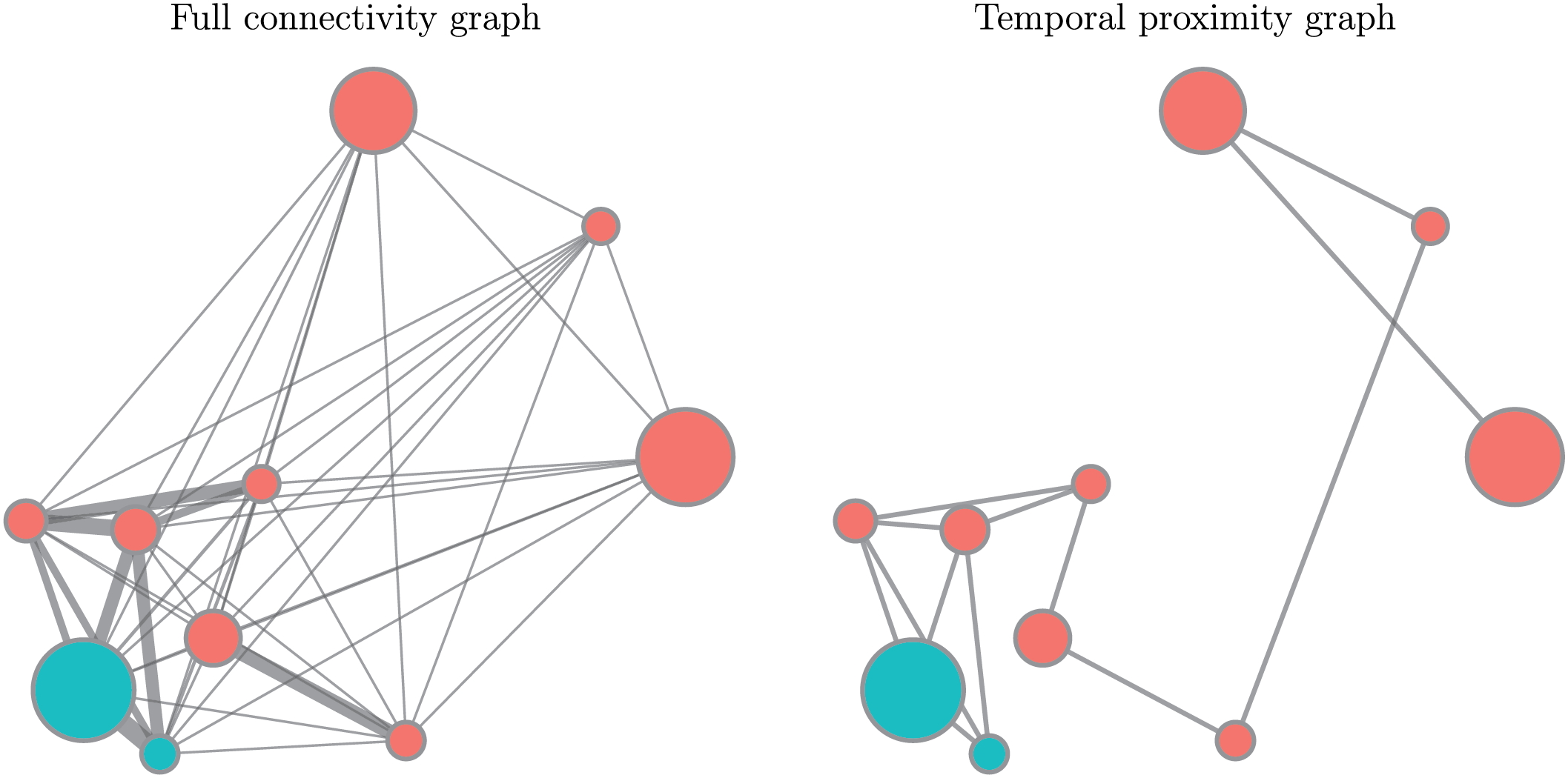
Figure 2: Transaction graphs for customer Katherine Tucker. For visualization clarity, only 10 representative transactions are shown from her total of 1250 transactions: 2 fraudulent transactions (blue) occurring on 15 January 2020, and 8 legitimate transactions (red) spanning from 16 March 2019 to 30 December 2019. Node size corresponds to transaction amount, and edge thickness represents temporal proximity. The left panel shows the full connectivity graph; the right panel shows the graph with only temporally close edges retained

The left panel shows a fully connected graph where all transactions are linked. Fraudulent transactions tend to cluster together temporally, forming tightly connected subgraphs. The right panel retains only edges between temporally close transactions, providing a sparser structure that highlights the temporal clustering of fraud.

4  Proposed Method

4.1 General Methodology

Let’s say the given data is X and y, where X is a n×p matrix and y is a vector of length n. Here, y contains labels, while X is the design matrix necessary for predicting y. Some columns of X can define relationships between different observations. Let’s denote one of these variables as xj. Here, j is the index of the variable selected to define relationships between observations. Let Wj represent the relationships measured between observations from xj by an appropriate method. In this context, Wj is an n×n matrix.

Our goal is to predict y by considering both X and W1,…,W|J|, where J is the index set of j and |J| is its cardinality. Since the dimension of Wj increases with n, it is necessary to reduce the size of Wj appropriately. For this purpose, we use the hidden layer Hj(Lj) learned from the graph convolution filter: Hj(l+1)=σ(Dj−1/2AjDj−1/2Hj(l)Θj(l)) for l=0,1,2,…,Lj−1. Here, Aj is the adjacency matrix corresponding to Wj and Dj is the degree matrix of Aj, Θj(l) represents the learnable parameters, and σ denotes the activation function. To learn Θj(l), we use a loss function similar to the one considered in [20]: ℒj=ℒ0+λℒjreg, where ℒjreg=oj⊤(Dj−Aj)oj. oj represents the output obtained by linearly transforming Hj(Lj). In a typical GCN, the last layer is a graph convolution layer. However, since our goal is to utilize the hidden layer as a new feature, the final transformation is performed using a standard linear transform instead of a graph convolution unit. This is to fully embed the connection information of the observations in the penultimate hidden layer. ℒ0 represents the supervised loss with respect to the labeled part of y, and ℒreg implies a constraint that makes values more similar as the relationship between observations increases. Hj(l) is the input for the lth layer, and Hj(l+1) is the output. When l=0, Hj(0) is defined as X(−j), where X(−j) represents the set of selected variables from the entire explanatory variable X, explicitly excluding xj. The output of the final layer is defined as y. Ultimately, an appropriate tabular model MTabular is trained by considering X~=X⊕H1(L1)⊕H2(L2)⊕⋯⊕H|J|(|J|) as explanatory variables to fit y. Here, ⊕ denotes concatenation. |J| represents the cardinality of the set J, which is the set of variables defining relationships among observations. The model MTabular can be any tabular classifier, such as XGBoost, LightGBM, etc. Algorithm 1 summarizes the proposed procedure, and the overall architecture is illustrated in Fig. 3.

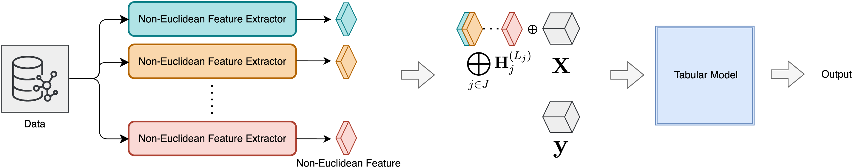
Figure 3: Overall architecture of the proposed framework. Multiple non-Euclidean feature extractors generate graph-based representations from the input data, which are aggregated and combined with original tabular features. The resulting features are then fed into a tabular model to produce the final output

Having established the general framework for graph-augmented feature learning, we now demonstrate its concrete application to credit card fraud detection. The following subsection specifies the graph construction, feature definitions, and model configuration tailored to our fraud detection task.

4.2 Application to Fraud Data

In this section, we will describe a model for analyzing fraud data using the methodology proposed in the previous section. Let the given data be denoted as (X,y). We interpret the given data as a graph. Here, we assume that the only column capturing the graph structure is trans_date_and_time (thus, |J|=1), and we will refer to it as xtime. Therefore, the relationships in the graph can be summarized by Wtime, and our task can be summarized as predicting y using X and Wtime.

The loss function ℒ=ℒ0+λℒreg is designed as follows. Here, ℒ0 is the Binary Cross-Entropy (BCE) loss: ℒ0=−1n∑i=1n(yilog⁡(y^i)+(1−yi)log⁡(1−y^i)), where y^i is the output of the GCN model. Additionally, ℒreg=y^⊤(Dtime−Atime)y^=∑i,jWtime,ij(y^i−y^j)2. This term represents a regularization component that enforces smoothness in the predictions. Specifically, it penalizes the model when the predicted values y^i and y^j for two observations that are close in time are significantly different. Here, Dtime is the degree matrix, Atime is the adjacency matrix, and Wtime,ij indicates the weight or connection strength between observations i and j. The term ∑i,jWtime,ij(y^i−y^j)2 ensures that the predictions for closely related observations (i.e., those with a strong connection in the graph) are similar.

Now, let’s describe in more detail how to compute Wtime. To create a weight matrix corresponding to xtime, we consider cc_num because even if transactions are temporally close, if they are made by different customer numbers, it is correct not to consider their connectivity. Therefore, Wtime will have a block-matrix structure: Wtime=diag(Wtime,1,Wtime,2,…,Wtime,|I|). Here, I is the set of cc_num. For a fixed i∈I, the (t,s)-th elements of Wtime,i are defined as follows, as used in [28]: Wtime,i(t,s)=exp⁡(−|t−s|2/ϕ) if t,s∈Ti, and 0 otherwise. In this context, Ti represents the set of transaction times for the i-th customer. The parameter ϕ is a positive constant that scales the time difference. A larger value in the exponential function indicates that the transaction times are closer together. To summarize, the weight matrix Wtime is constructed by considering both the temporal proximity and the customer number. Each block matrix Wtime,i within Wtime represents the temporal relationships between transactions for a specific customer. Transactions from different customers are not connected, which is reflected in the block-diagonal structure of Wtime.

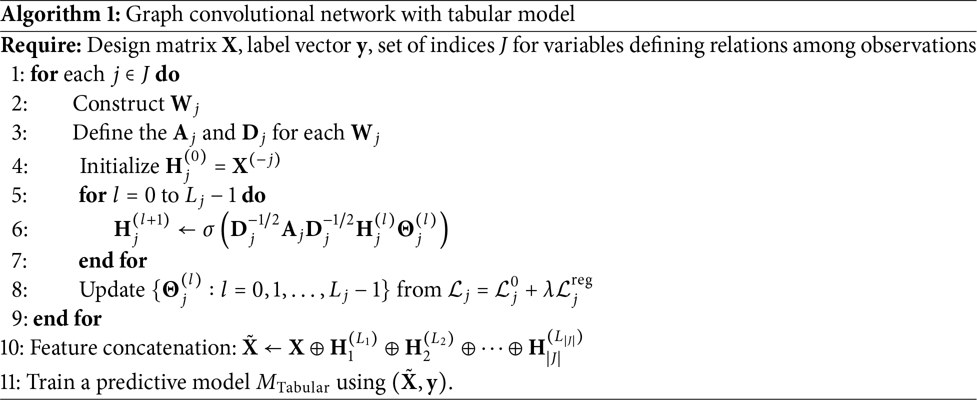
We have configured the architecture as shown in Fig. 4 to obtain the hidden layer.

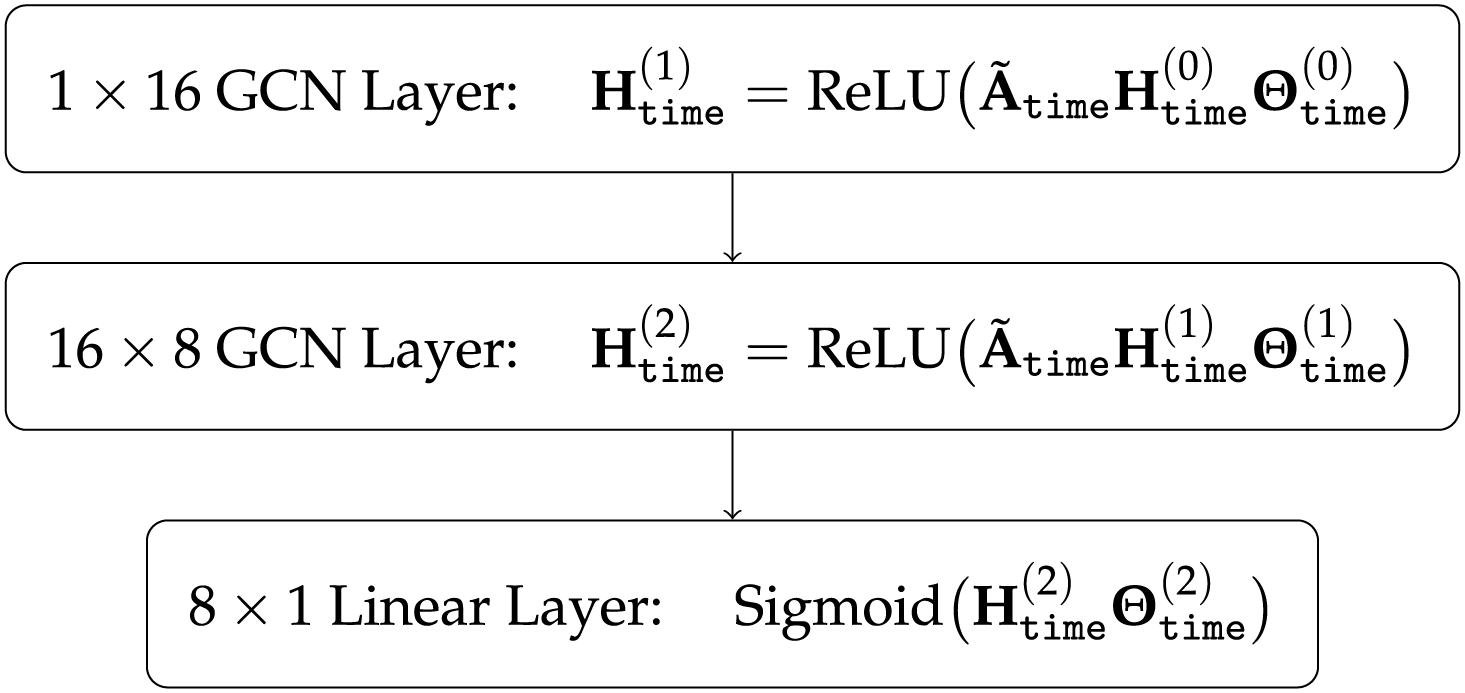
Figure 4: GCN architecture for extracting non-Euclidean features. Here A~time=Dtime−1/2AtimeDtime−1/2 is the normalized adjacency matrix. The input Htime(0) consists of the transaction amount xamt, processed through two GCN layers to produce an 8-dimensional representation Htime(2)

Here Htime(0) consists solely of xamt, since amt is the most crucial factor in predicting fraud. A typical GCN architecture uses an 8×1 GCN Layer instead of the final Linear Layer. However, our objective is to obtain the n×8 matrix Htime(2) for concatenation with the original feature matrix X (which includes variables not used for graph construction), so we chose a Linear Layer solely for dimension reduction, sacrificing prediction performance in order to fully capture non-Euclidean information in Htime(2).

5  Experiment & Results

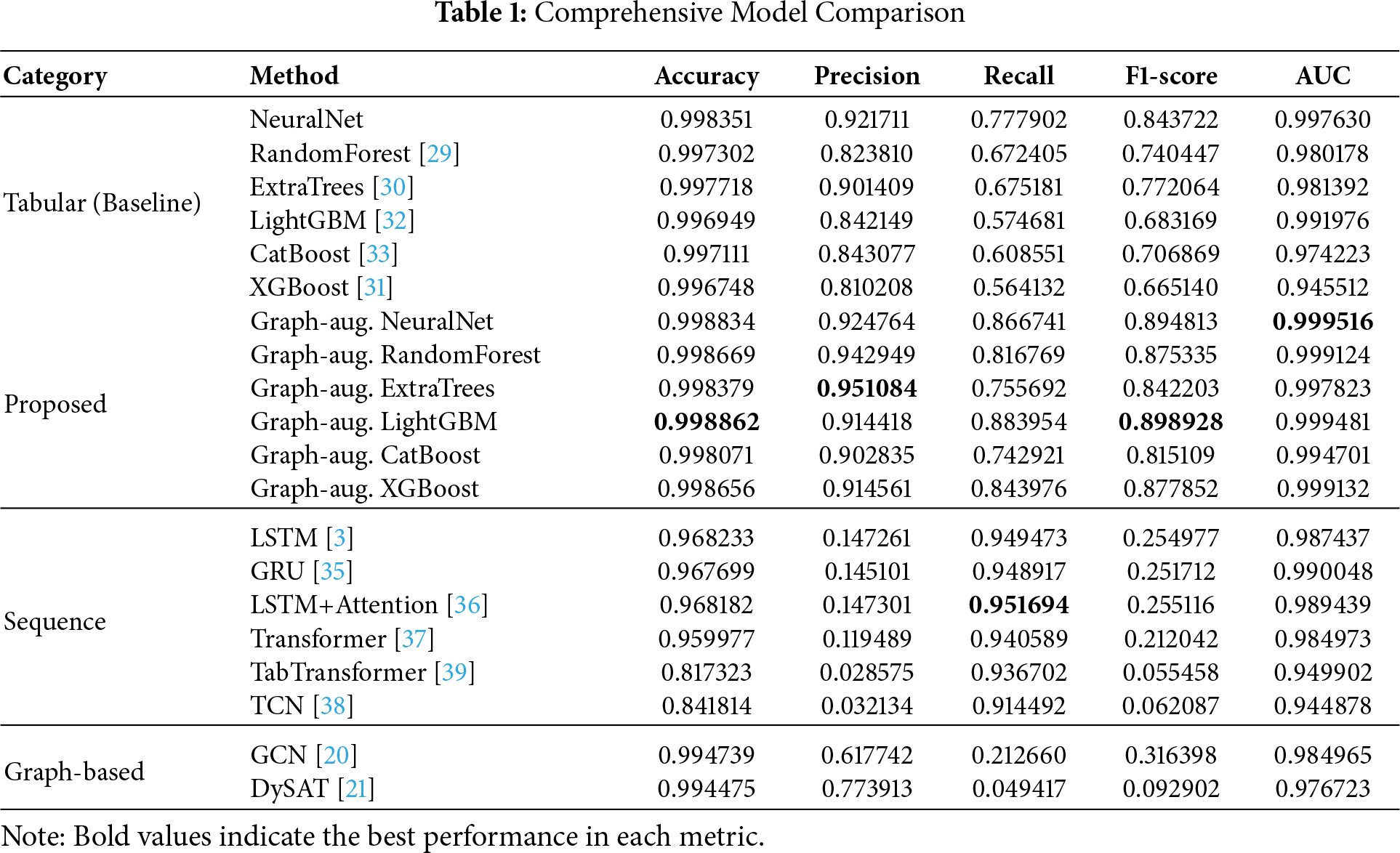
We evaluate our proposed graph-augmented approach using six baseline tabular models: NeuralNet (PyTorch-based MLP), RandomForest [29], ExtraTrees [30], XGBoost [31], LightGBM [32], and CatBoost [33]. The baseline models were trained using AutoGluon-Tabular [34], an automated machine learning framework.

5.1 Overall Performance Comparison

We conducted comprehensive experiments to evaluate our proposed method against three categories of approaches: (i) conventional tabular models as baselines, (ii) the same tabular models augmented with GCN embeddings (our proposed approach), (iii) sequence-based architectures including GRU [35], LSTM with attention [36], Transformer-based models [37], and temporal convolutional networks (TCN) [38], and (iv) graph-based models such as GCN [20] and DySAT [21].

The results reveal important findings across model categories. Baseline tabular models already achieve strong performance (NeuralNet AUC 0.997, ensemble models 0.94–0.99), maintaining high precision (above 0.90) but with relatively lower recall (0.21–0.77). Sequence models achieve competitive Area Under Curve (AUC) (GRU 0.990, LSTM 0.988, Transformer 0.985), but despite high recall (above 0.91), they suffer from very low precision (below 0.15), exhibiting a precision-recall trade-off. Graph-based models (GCN AUC 0.985, DySAT AUC 0.977) directly utilize graph structure for classification but show lower performance than baseline tabular models.

In contrast, our proposed graph-augmented models achieve the highest performance by using GCN embeddings as additional features for tabular models: graph-augmented NeuralNet attains AUC of 0.9995, outperforming all other methods, consistently improving all baseline models (AUC improvement: 0.002–0.054), and achieving both high precision (above 0.90) and improved recall for balanced performance. This superior performance can be attributed to the following: (1) compared to tabular models, graph embeddings provide temporal proximity information between transactions that tabular features alone cannot capture, improving recall; (2) compared to sequence models, using GCN embeddings as features rather than as the classifier preserves the stable precision of tabular models while incorporating graph information; and (3) compared to pure graph-based models, extracting graph features and then applying well-established tabular classifiers achieves better generalization than performing both feature extraction and classification in non-Euclidean space.

These results cannot be directly generalized to fraud detection in general. The optimal model may vary depending on the fraud transaction ratio, characteristics of fraud patterns, and temporal structure of the data. However, our proposed method holds unique significance in that it appropriately combines the stable precision of tabular models, the sequential pattern capturing capability of sequence models, and the relational information utilization of graph models.

5.2 Prediction Confidence Analysis

AUC is a useful threshold-independent metric for evaluating the overall discriminative ability of classifiers. However, in extreme class imbalance settings, F1-score also warrants consideration. As shown in Table 1, baseline Euclidean models achieve high precision (0.81–0.92) but relatively low recall (0.21–0.78)—this occurs because they primarily detect “certain” fraud cases with high transaction amounts. In contrast, our proposed graph-augmented models maintain precision (0.91–0.95) while improving recall (0.76–0.88), showing improvements in F1-score (0.84–0.90). To analyze specifically where these AUC and F1-score improvements originate, we examine prediction confidence.

While the overall AUC values show modest improvements due to already well-trained baseline models, the practical benefit becomes more pronounced when examining predictions for low-amount transactions. Fig. 5 presents a comprehensive comparison of predicted probabilities for actual fraud cases (y=1) using the LightGBM model (results for other models are available in the supplementary materials). The top row shows histograms: the proposed model (orange) concentrates predictions near 1.0, indicating high confidence, while the classic model (blue) spreads predictions across a wider range. This difference is particularly striking for low-amount transactions (amt <80), where the classic model shows a bimodal distribution with many predictions near 0, whereas the proposed model maintains confident predictions near 1.0.

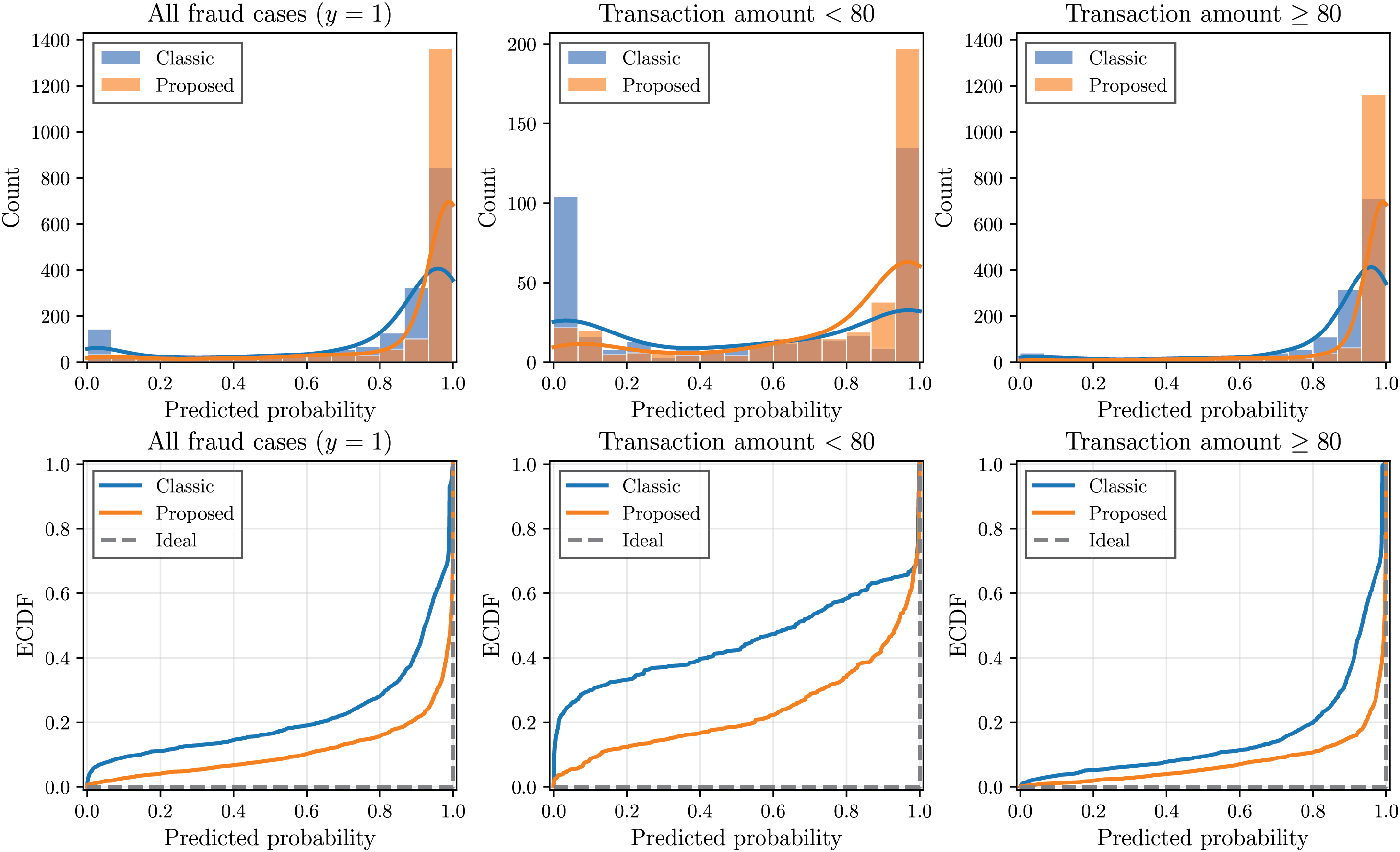
Figure 5: Comparison of predicted fraud probabilities for actual fraud cases (y=1). Top row: histograms showing prediction distributions; bottom row: empirical cumulative distribution functions (empirical CDF). Columns show all fraud cases (left), low-amount transactions with amt <80 (middle), and high-amount transactions with amt ≥80 (right). The classic model (blue) uses only tabular features X, while the proposed model (orange) incorporates GCN embeddings X~. The dashed gray line in empirical CDF plots represents the ideal classifier. The proposed model consistently achieves predictions closer to 1.0, particularly for low-amount transactions where the classic model struggles

The bottom row of Fig. 5 presents the empirical cumulative distribution function (empirical CDF) of these predicted probabilities, providing a clearer comparison. For an ideal classifier, all fraud cases should receive a predicted probability of 1, resulting in a step function at probability =1 (dashed gray line). The closer a model’s empirical cumulative distribution function (CDF) is to this ideal step function, the more confidently it identifies fraud. The classic model (blue) shows a gradual increase across the probability range, indicating uncertainty in fraud detection, while the proposed model (orange) concentrates predictions near 1.0 with a median of 0.99 compared to 0.92 for the classic model. This improvement is particularly pronounced for low-amount transactions (amt <80) in the middle column, where the classic model’s empirical CDF rises steeply even at low probability values. The right column shows high-amount transactions (amt ≥80), where both models perform better, but the proposed model still achieves predictions closer to the ideal, confirming that graph-based embeddings provide additional discriminative power.

We present a visual example using Michael Rodriguez’s transactions, which include 249 test transactions with 4 fraudulent cases. Table 2 compares the baseline model predictions with our proposed graph-augmented model.

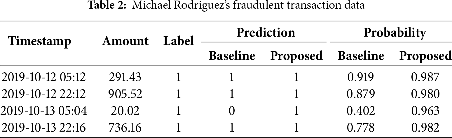
The average transaction amount for Michael Rodriguez is 56.25. The average amount for legitimate transactions is 49.19, while the average amount for fraudulent transactions is 488.28. In existing studies, all transactions with high amt values were predicted as fraudulent, but a transaction with a small amt value of 20.02 was predicted as legitimate. When amt is 20.02, the predicted probability is a low value of 0.4. In contrast, the method utilizing graph information correctly predicted the small amt transaction as fraudulent with a high probability value of 0.96. Moreover, this method showed higher probability values for high amt transactions compared to existing studies.

This can be more easily understood by examining Fig. 6, which visualizes the graph. It depicts nine transactions closely related to fraudulent transactions among Michael’s transactions. The graph shown is after removing links based on the weights of the edges. This method can adequately determine fraud even when the transaction amounts are small.

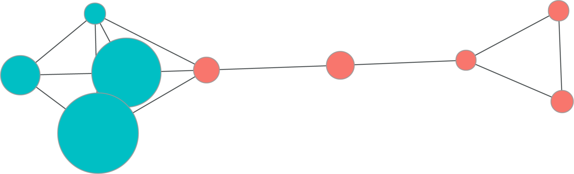
Figure 6: Graph representation of transaction patterns for customer Michael Rodriguez

5.3 Undersampling Experiments

In the previous experiments, we maintained the original fraud transaction ratio of 0.00573 with a 7:3 train-test split. However, dealing with such extreme class imbalance is a common challenge in fraud detection. A widely-used technique is undersampling, where the majority class (legitimate transactions) is reduced to achieve a more balanced training set while keeping the test set unchanged to reflect real-world conditions.

We conducted additional experiments with various undersampling ratios (fraud ratios from 0.05 to 0.5) to evaluate the robustness of our proposed method. The results consistently demonstrate that incorporating GCN embeddings into the feature set yields superior performance compared to using only the original features, regardless of the undersampling ratio. This validates the effectiveness of our approach when combined with standard class imbalance handling techniques. Detailed experimental settings and results are available in our supplementary materials.2

6  Theoretical Interpretation: GCN Embeddings as Temporal Random Effects

This section provides a theoretical framework for understanding why GCN embeddings improve fraud detection performance. We interpret the GCN embeddings as a replacement for traditional random effects in hierarchical models, and conduct statistical tests to validate the significance of their contribution.

To simplify the theoretical discussion and enable closed-form statistical testing, we use logistic regression as the downstream classifier with an undersampled dataset (n=8410, fraud ratio = 0.5). This choice is justified by the robustness analysis in the supplementary materials, which demonstrates that GCN embeddings provide consistent performance improvements across all six model types (NeuralNet, RandomForest, ExtraTrees, LightGBM, CatBoost, XGBoost) and all undersampling ratios (5%–50%). Therefore, insights derived from the logistic regression setting with an undersampled dataset (n=8410, fraud ratio = 0.5) generalize to the broader experimental spectrum.

Our graph-based approach models both temporal and customer information together. Temporal information can be extracted as features and placed in X, while customer effects can be considered through mixed effects models. Using the notation from Section 4, let X∈Rn×k denote the feature matrix and y∈{0,1}n the fraud indicators. For the j-th transaction of customer i, the traditional generalized linear mixed model with customer-level random effects is logit(P(yij=1))=β0+β⊤xij+ui, where ui∼N(0,σu2), xij is the j-th row of X corresponding to customer i, and ui represents the customer-specific random effect. This formulation assumes conditional independence of transactions given ui.

However, fraudulent transactions exhibit strong temporal clustering—multiple unauthorized charges typically occur within minutes before detection. Our proposed method replaces the customer random effect ui with a learned embedding: logit(P(yij=1))=β0+β⊤xij+γ⊤hij, where hij∈Rd is the GCN embedding for the j-th transaction of customer i, computed from customer i’s transaction graph. This embedding captures both customer-specific patterns (since it is derived from customer i’s own transaction history) and temporal proximity effects (since neighboring transactions with similar timestamps contribute more strongly). The augmented feature matrix is X~=X⊕H1(L1)⊕⋯⊕H|J|(L|J|) as defined in Algorithm 1.

Unlike random effects, the GCN embeddings are learned through message-passing and can be treated as fixed effects in the downstream classifier. To empirically validate this interpretation, we conducted an ablation study (n=8410, fraud ratio = 0.5, logistic regression). The baseline feature matrix X consists of k=6 continuous features: transaction amount (amt), customer location (lat, long), city population (city_pop), and merchant location (merch_lat, merch_long). These features were selected because they represent the core numerical attributes available for each transaction and are commonly used in fraud detection literature. We also tested adding explicit temporal features (trans_hour, trans_day_of_week) as direct features, but found they provide negligible improvement. This is because temporal information is more effectively captured through the graph structure: the edge weights of the transaction graph encode temporal proximity, and the GCN embeddings H(L) learn to exploit this relational structure. The results are summarized in Table 3.

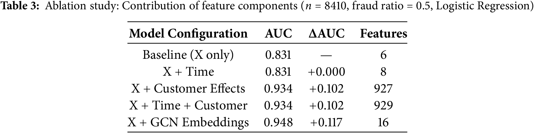
As shown in Table 3, GCN embeddings achieve superior performance (+0.117 AUC improvement) with only 16 features, compared to customer dummies which require 927 features for a +0.102 improvement.

Notably, explicit temporal features (trans_hour, trans_day_of_week) provide essentially no improvement. This reveals a fundamental distinction between two types of temporal patterns. Absolute temporal patterns refer to statements like “transactions at 23:00 are more likely to be fraudulent,” which would require fraud to concentrate at specific hours or days—a pattern largely absent in our data. In contrast, relative temporal patterns refer to statements like “a transaction temporally close to a fraudulent transaction is also likely to be fraudulent”—this fraud clustering pattern is precisely what our data exhibits.

Conventional feature engineering cannot easily capture relative temporal patterns because doing so would require knowing the fraud labels of neighboring transactions a priori. Our GCN-based approach elegantly solves this: the graph structure encodes temporal proximity between transactions, and the message-passing mechanism allows fraud-related signals to propagate through temporally adjacent nodes during training. This explains why the relational structure of temporal proximity—not raw timestamp values—is the key to improved fraud detection. To formally test significance, let f denote the logistic regression classifier. We compare baseline model ℳ0:y^=f(X) against the augmented model ℳ1:y^=f(X~), where X~ is defined as in Algorithm 1. In our experimental setting: n=8410 (sample size), k=8 (number of baseline features in X, including temporal features), and d=8 (GCN embedding dimensions).

Under H0: “GCN embeddings do not contribute,” the likelihood ratio statistic follows Λ=2(ℓ1−ℓ0)→dχd2 asymptotically. This approximation requires regularity conditions, which we verify in Table 4. The first condition ensures adequate sample size relative to the total number of features (k+d=16). The second condition is satisfied by construction since X~ contains all columns of X.

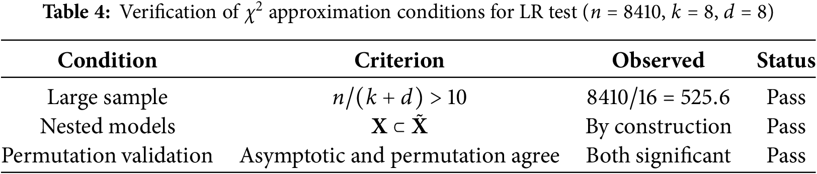
Finally, we validate the asymptotic χ2 approximation through a permutation test. By randomly permuting the GCN embeddings (100 iterations), we break any true association with the outcome and obtain the null distribution of Λ. Under the null hypothesis where GCN embeddings have no predictive value, this distribution has mean μ=7.11 and standard deviation σ=3.59. Our observed statistic Λ=2719.92 lies approximately 756 standard deviations above this null mean, providing strong evidence against H0: Λ=2719.92≫χ8,0.0012=26.12(asymptotic p<0.001, permutation p<0.0001).The partial F-test confirms these findings: F=(SSE0−SSE1)/dSSE1/(n−k−d)=837.23 (p-value <0.001), ΔR2=0.231.

These tests confirm that GCN embeddings provide statistically significant predictive value by capturing temporal dependencies that traditional methods overlook.

7  Conclusion

7.1 Why Graph-Augmented Features Work

Sequence-based approaches (LSTM, Gated Recurrent Unit (GRU), Transformer) assume equally-spaced time intervals, but credit card transactions occur at irregular intervals—ranging from seconds apart during shopping sessions to days or weeks between purchases. Moreover, these models process transactions as ordered sequences without modeling the connectivity structure between temporally proximate transactions. Our graph-based approach explicitly captures irregular temporal relationships through edge weights that encode temporal proximity, naturally handling non-uniform time spacing without requiring temporal discretization or padding.

While non-Euclidean approaches can capture temporal and customer dependencies, they introduce unnecessary complexity. In practice, the vast majority of legitimate transactions can be correctly classified using Euclidean features alone—temporal clustering patterns become critical only in the vicinity of fraudulent activity. A purely graph-based model would be computationally expensive and may overfit to relational patterns irrelevant for normal transactions. Our analysis shows that GCN embeddings contribute an additional 23.1% of explained variance (ΔR2=0.231), but this contribution is localized to fraud-adjacent regions rather than uniformly distributed across all transactions.

Our approach offers an elegant middle ground. The base Euclidean classifier efficiently handles the majority of straightforward cases, while GCN embeddings provide supplementary non-Euclidean information precisely where it matters—near fraud clusters. This design avoids the overhead of full graph-based inference while retaining the benefits of temporal dependency modeling. The concatenation allows the downstream classifier to adaptively weight Euclidean vs. non-Euclidean features based on context, achieving both high precision (above 0.90) and improved recall without the computational burden of end-to-end graph models. Furthermore, this modular design offers practical advantages: the GCN embedding generation is independent of the downstream classifier, allowing practitioners to leverage existing classification infrastructure while benefiting from graph-based feature augmentation.

7.2 Limitations and Future Work

While our proposed method demonstrates strong performance on the analyzed dataset, several limitations should be acknowledged. First, our evaluation is based on a single publicly available dataset that may not fully represent the diversity of fraud patterns encountered in real-world financial systems. Credit card fraud datasets vary significantly in their characteristics: some contain only anonymized features and lack explicit temporal information. The generalizability of our method to these diverse fraud scenarios requires further validation. Second, our approach constructs individual graphs for each customer, which assumes sufficient transaction history per customer. For customers with very few transactions, the graph structure may be too sparse to provide meaningful embeddings. Third, our approach assumes that temporal proximity is the primary factor determining transaction relationships, which may not hold in all fraud scenarios—for instance, when fraudsters deliberately introduce time delays between fraudulent activities. Future work could address these limitations by: (i) evaluating on multiple fraud datasets with different characteristics, (ii) developing adaptive methods for customers with limited transaction history, and (iii) exploring alternative kernel functions that capture more complex temporal patterns.

Acknowledgement: Not applicable.

Funding Statement: This research was supported by the National Research Foundation of Korea (NRF) funded by the Korea government (RS-2023-00249743). Additionally, this research was supported by the Global-Learning & Academic Research Institution for Master’s, PhD Students, and Postdocs (LAMP) Program of the National Research Foundation of Korea (NRF) grant funded by the Ministry of Education (RS-2024-00443714). This research was also supported by the “Research Base Construction Fund Support Program” funded by Jeonbuk National University in 2025.

Author Contributions: Conceptualization and methodology, Guebin Choi; software, validation, formal analysis, investigation, data curation, visualization, and writing—original draft, Boram Kim; writing—review and editing, Guebin Choi and Boram Kim; supervision and funding acquisition, Guebin Choi. All authors reviewed the results and approved the final version of the manuscript.

Availability of Data and Materials: The data that support the findings of this study are openly available in Kaggle at https://www.kaggle.com/datasets/dermisfit/fraud-transactions-dataset. Supplementary materials including detailed experimental results are available at https://guebin.github.io/non-euclidean-models-for-fraud-detection/.

Ethics Approval: Not applicable.

Conflicts of Interest: The authors declare no conflicts of interest to report regarding the present study.

1https://www.kaggle.com/datasets/dermisfit/fraud-transactions-dataset

2https://guebin.github.io/non-euclidean-models-for-fraud-detection/

References

1. Nilson Report. Global card fraud losses reach $403.88 Billion. 2025 [cited 2025 Jan 15]. Available from: https://nilsonreport.com. [Google Scholar]

2. Whitrow C, Hand DJ, Juszczak P, Weston D, Adams NM. Transaction aggregation as a strategy for credit card fraud detection. Data Min Knowl Discov. 2009;18(1):30–55. doi:10.1007/s10618-008-0116-z. [Google Scholar] [CrossRef]

3. Hochreiter S, Schmidhuber J. Long short-term memory. Neural Comput. 1997;9(8):1735–80. doi:10.1162/neco.1997.9.8.1735. [Google Scholar] [PubMed] [CrossRef]

4. Krawczyk B. Learning from imbalanced data: open challenges and future directions. Prog Artif Intell. 2016;5(4):221–32. doi:10.1007/s13748-016-0094-0. [Google Scholar] [CrossRef]

5. Makki S, Assaghir Z, Taher Y, Haque R, Hacid MS, Zeineddine H. An experimental study with imbalanced classification approaches for credit card fraud detection. IEEE Access. 2019;7:93010–22. doi:10.1109/access.2019.2927266. [Google Scholar] [CrossRef]

6. Alam TM, Shaukat K, Hameed IA, Luo S, Sarwar MU, Shabbir S, et al. An investigation of credit card default prediction in the imbalanced datasets. IEEE Access. 2020;8:201173–98. doi:10.1109/access.2020.3033784. [Google Scholar] [CrossRef]

7. Wei W, Li J, Cao L, Ou Y, Chen J. Effective detection of sophisticated online banking fraud on extremely imbalanced data. World Wide Web. 2013;16(4):449–75. doi:10.1007/s11280-012-0178-0. [Google Scholar] [CrossRef]

8. Tayebi M, El Kafhali S. Combining autoencoders and deep learning for effective fraud detection in credit card transactions. Oper Res Forum. 2025;6(1):8. doi:10.1007/s43069-024-00409-6. [Google Scholar] [CrossRef]

9. Tayebi M, El Kafhali S. Generative modeling for imbalanced credit card fraud transaction detection. J Cybersecur Priv. 2025;5(1):9. doi:10.3390/jcp5010009. [Google Scholar] [CrossRef]

10. Van Vlasselaer V, Bravo C, Caelen O, Eliassi-Rad T, Akoglu L, Snoeck M, et al. APATE: a novel approach for automated credit card transaction fraud detection using network-based extensions. Decis Support Syst. 2015;75(3):38–48. doi:10.1016/j.dss.2015.04.013. [Google Scholar] [CrossRef]

11. Stamile C, Marzullo A, Deusebio E. Graph machine learning: take graph data to the next level by applying machine learning techniques and algorithms. Birmingham, UK: Packt Publishing Ltd.; 2021. [Google Scholar]

12. Weber M, Domeniconi G, Chen J, Weidele DKI, Bellei C, Robinson T, et al. Anti-money laundering in bitcoin: experimenting with graph convolutional networks for financial forensics. arXiv:1908.02591. 2019. [Google Scholar]

13. Grover A, Leskovec J. node2vec: scalable feature learning for networks. In: Proceedings of the 22nd ACM SIGKDD International Conference on Knowledge Discovery and Data Mining; New York, NY, USA: ACM; 2016. p. 855–64. [Google Scholar]

14. Zhang Q, Yan B, Huang M. Internet financial fraud detection based on a distributed big data approach with Node2vec. IEEE Access. 2021;9:43378–86. doi:10.1109/access.2021.3062467. [Google Scholar] [CrossRef]

15. Bruss CB, McGee A, Muench B, Chaluvaraju P, Rajput S. DeepTrax: embedding graphs of financial transactions. In: 2019 18th IEEE International Conference on Machine Learning and Applications (ICMLA); Piscataway, NJ, USA: IEEE; 2019. p. 126–33. [Google Scholar]

16. Wang Y, Zhang X, Chen L. Heterogeneous graph auto-encoder for credit card fraud detection. arXiv:2410.08121. 2024. [Google Scholar]

17. Benchaji I, Douzi S, El Ouahidi B. Credit card fraud detection model based on LSTM recurrent neural networks. J Adv Inf Technol. 2021;12(2):113–8. doi:10.12720/jait.12.2.113-118. [Google Scholar] [CrossRef]

18. Alarfaj FK, Malik I, Khan HU, Almusallam N, Ramzan M, Ahmed M. Credit card fraud detection using state-of-the-art machine learning and deep learning algorithms. IEEE Access. 2022;10:39700–15. doi:10.1109/access.2022.3166891. [Google Scholar] [CrossRef]

19. Yu C, Xu Y, Cao J, Zhang Y, Jin Y, Zhu M. Credit card fraud detection using advanced transformer model. arXiv:2406.03733. 2024. [Google Scholar]

20. Kipf TN, Welling M. Semi-supervised classification with graph convolutional networks. arXiv:1609.02907. 2016. [Google Scholar]

21. Sankar A, Wu Y, Gou L, Zhang W, Yang H. DySAT: deep neural representation learning on dynamic graphs via self-attention networks. In: Proceedings of the 13th International Conference on Web Search and Data Mining; New York, NY, USA: ACM; 2020. p. 519–27. [Google Scholar]

22. You J, Du T, Leskovec J. ROLAND: graph learning framework for dynamic graphs. In: Proceedings of the 28th ACM SIGKDD Conference on Knowledge Discovery and Data Mining; New York, NY, USA: ACM; 2022. p. 2358–66. [Google Scholar]

23. Cheng Y, Liu C, Liu Y. CaT-GNN: enhancing credit card fraud detection via causal temporal graph neural networks. arXiv:2402.14708. 2024. [Google Scholar]

24. Wheeler R, Aitken S. Multiple algorithms for fraud detection. In: Applications and Innovations in Intelligent Systems VII: Proceedings of ES99, the Nineteenth SGES International Conference on Knowledge Based Systems and Applied Artificial Intelligence; Cham, Switzerland: Springer; 2000. p. 219–31. [Google Scholar]

25. Srivastava A, Kundu A, Sural S, Majumdar A. Credit card fraud detection using hidden Markov model. IEEE Trans Dependable Secure Comput. 2008;5(1):37–48. doi:10.1109/tdsc.2007.70228. [Google Scholar] [CrossRef]

26. Sánchez D, Vila M, Cerda L, Serrano JM. Association rules applied to credit card fraud detection. Exp Syst Appl. 2009;36(2):3630–40. doi:10.1016/j.eswa.2008.02.001. [Google Scholar] [CrossRef]

27. Liu T, Zhang W, Chen J. Effective high-order graph representation learning for credit card fraud detection. arXiv:2503.01556. 2025. [Google Scholar]

28. Shuman DI, Narang SK, Frossard P, Ortega A, Vandergheynst P. The emerging field of signal processing on graphs: extending high-dimensional data analysis to networks and other irregular domains. IEEE Signal Process Mag. 2013;30(3):83–98. doi:10.1109/msp.2012.2235192. [Google Scholar] [CrossRef]

29. Liaw A, Wiener M. Classification and regression by randomForest. R News. 2002;2(3):18–22. [Google Scholar]

30. Geurts P, Ernst D, Wehenkel L. Extremely randomized trees. Mach Learn. 2006;63(1):3–42. doi:10.1007/s10994-006-6226-1. [Google Scholar] [CrossRef]

31. Chen T, Guestrin C. Xgboost: a scalable tree boosting system. In: Proceedings of the 22nd ACM SIGKDD International Conference on Knowledge Discovery and Data Mining; New York, NY, USA: ACM; 2016. p. 785–94. [Google Scholar]

32. Ke G, Meng Q, Finley T, Wang T, Chen W, Ma W, et al. Lightgbm: a highly efficient gradient boosting decision tree. Vol. 30. In: Advances in neural information processing systems. Red Hook, NY, USA: Curran Associates, Inc.; 2017. doi:10.32614/cran.package.lightgbm. [Google Scholar] [CrossRef]

33. Prokhorenkova L, Gusev G, Vorobev A, Dorogush AV, Gulin A. CatBoost: unbiased boosting with categorical features. Vol. 31. In: Advances in neural information processing systems. Red Hook, NY, USA: Curran Associates, Inc.; 2018. [Google Scholar]

34. Erickson N, Mueller J, Shirkov A, Zhang H, Larroy P, Li M, et al. AutoGluon-Tabular: robust and accurate AutoML for structured data. arXiv:2003.06505. 2020. [Google Scholar]

35. Cho K, Van Merriënboer B, Gulcehre C, Bahdanau D, Bougares F, Schwenk H, et al. Learning phrase representations using RNN encoder-decoder for statistical machine translation. In: Proceedings of the 2014 Conference on Empirical Methods in Natural Language Processing (EMNLP); Stroudsburg, PA, USA: ACL; 2014. p. 1724–34. [Google Scholar]

36. Bahdanau D, Cho K, Bengio Y. Neural machine translation by jointly learning to align and translate. arXiv:1409.0473. 2015. [Google Scholar]

37. Vaswani A, Shazeer N, Parmar N, Uszkoreit J, Jones L, Gomez AN, et al. Attention is all you need. In: Advances in neural information processing systems. Vol. 30. Red Hook, NY, USA: Curran Associates, Inc.; 2017. doi:10.65215/ctdc8e75. [Google Scholar] [CrossRef]

38. Bai S, Kolter JZ, Koltun V. An empirical evaluation of generic convolutional and recurrent networks for sequence modeling. arXiv:1803.01271. 2018. [Google Scholar]

39. Huang X, Khetan A, Cvitkovic M, Karnin Z. TabTransformer: tabular data modeling using contextual embeddings. arXiv:2012.06678. 2020. [Google Scholar]