
 Submit a Paper
 Propose a Special lssue
 Open Access
ARTICLE
HMA-DER: A Hierarchical Attention and Expert Routing Framework for Accurate Gastrointestinal Disease Diagnosis
1 Faculty of Informatics, Kaunas University of Technology, Kaunas, 51368, Lithuania
2 College of Engineering and Technology, American University of the Middle East, Egaila, 54200, Kuwait
3 Department of Computer Sciences, College of Computer and Information Sciences, Princess Nourah bint Abdulrahman University, P.O. Box 84428, Riyadh, 11671, Saudi Arabia
4 Department of Computer Science and Artificial Intelligence, College of Computer Science and Engineering, University of Jeddah, Jeddah, 23890, Saudi Arabia
5 Department of Computer Science, Applied College, Shaqra University, Shaqra, 15526, Saudi Arabia
6 Department of Information Systems, College of Computer and Information Sciences, Princess Nourah bint Abdulrahman University, P.O. Box 84428, Riyadh, 11671, Saudi Arabia
* Corresponding Author: Inzamam Mashood Nasir. Email:
Computers, Materials & Continua 2026, 87(1), 26 https://doi.org/10.32604/cmc.2025.074416
Received 10 October 2025; Accepted 17 November 2025; Issue published 10 February 2026
 View Full Text
 Download PDF
Abstract
Objective: Deep learning is employed increasingly in Gastroenterology (GI) endoscopy computer-aided diagnostics for polyp segmentation and multi-class disease detection. In the real world, implementation requires high accuracy, therapeutically relevant explanations, strong calibration, domain generalization, and efficiency. Current Convolutional Neural Network (CNN) and transformer models compromise border precision and global context, generate attention maps that fail to align with expert reasoning, deteriorate during cross-center changes, and exhibit inadequate calibration, hence diminishing clinical trust. Methods: HMA-DER is a hierarchical multi-attention architecture that uses dilation-enhanced residual blocks and an explainability-aware Cognitive Alignment Score (CAS) regularizer to directly align attribution maps with reasoning signals from experts. The framework has additions that make it more resilient and a way to test for accuracy, macro-averaged F1 score, Area Under the Receiver Operating Characteristic Curve (AUROC), calibration (Expected Calibration Error (ECE), Brier Score), explainability (CAS, insertion/deletion AUC), cross-dataset transfer, and throughput. Results: HMA-DER gets Dice Similarity Coefficient scores of 89.5% and 86.0% on Kvasir-SEG and CVC-ClinicDB, beating the strongest baseline by +1.9 and +1.7 points. It gets 86.4% and 85.3% macro-F1 and 94.0% and 93.4% AUROC on HyperKvasir and GastroVision, which is better than the baseline by +1.4/+1.6 macro-F1 and +1.2/+1.1 AUROC. Ablation study shows that hierarchical attention gives the highest (+3.0), followed by CAS regularization (+2–3), dilatation (+1.5–2.0), and residual connections (+2–3). Cross-dataset validation demonstrates competitive zero-shot transfer (e.g., KSKeywords
Deep learning has improved computer-aided diagnosis (CAD) for gastrointestinal (GI) endoscopy, allowing for polyp segmentation and the detection of many disease classes in different clinical settings. There are a number of public datasets, including Kvasir-SEG (KS) for pixel-level polyp delineation [1], CVC-ClinicDB (CVC) for benchmark segmentation in difficult imaging conditions [2,3], HyperKvasir (HK) for large-scale, heterogeneous classification [4], and GastroVision (GV) for curated multi-class diagnosis [5]. Even while accuracy has gotten better, routine clinical use still needs calibrated probability, robustness to domain shifts, and explanations that are in line with what humans would expect to generate trust in the system.
Residual and densely linked networks have enhanced optimization and feature reuse in medical imaging, creating robust baselines [6,7]. Newer vision transformers, such as ViT and Swin, have shown higher performance thanks to global self-attention. Hybrid designs, like TransUNet [8] and MedT, combine convolutional priors with transformer modules to better model context in medical pictures [8,9]. Three things make it hard to use GI CAD: (i) getting accurate estimates of fine lesion borders and long-range context without overfitting; (ii) giving calibrated confidence estimates for making decisions based on risk; and (iii) keeping accuracy when cross-center distribution shifts and common corruptions happen.
To highlight the novelty and significance of this work, the key contributions of the proposed HMA-DER framework are summarized as follows:
• We introduce HMA-DER, a unified framework that combines Hierarchical Multi-Attention (HMA) with Dynamic Expert Routing (DER) to achieve accurate and explainable gastrointestinal (GI) disease diagnosis from endoscopic images.
• A hierarchical multi-attention system collects information that is useful at the global, regional, and local levels. This helps the model focus on clinically important features, including polyps, ulcer boundaries, bleeding, and irritated mucosa, while getting rid of background noise.
• Dynamic expert routing sends low-confidence or complicated samples to specialized expert networks to make classification more reliable and cut down on diagnostic mistakes like false negatives and positives.
• The integrated explainability module inherently performs lesion localization during classification, producing interpretable attention maps that align closely with expert-annotated lesion regions.
• The system for segmentation and multi-class classification is tested using four complimentary benchmark datasets: Kvasir-SEG, CVC-ClinicDB, HyperKvasir, and GastroVision. HMA-DER often beats advanced CNN and Transformer baselines.
• Ablation experiments demonstrate the efficacy of the hierarchical attention and expert routing modules, while clinical alignment metrics indicate that the model’s attention correlates with actual pathological structures.
• The proposed system establishes a practical step toward clinically trustworthy computer-aided diagnosis by combining high diagnostic accuracy with interpretable, anatomically grounded visual reasoning.
The structure of this paper continues below. Section 2 looks at deep learning research on diagnosing gastrointestinal diseases, focusing on attention mechanisms and expert systems. In Section 3, we talk about the HMA-DER framework’s hierarchical multi-attention architecture and dynamic expert routing method. Section 4 talks about the datasets, implementation settings, evaluation criteria, and experimental findings. These include ablation experiments and clinical alignment studies. In Section 5, the study ends with important results and ideas for further research.
Computer-aided diagnosis (CAD) for gastrointestinal endoscopy has progressed swiftly owing to deep learning, with public datasets for reproducible benchmarking in segmentation and classification tasks. Kvasir-SEG and CVC-ClinicDB standardize polyp delineation at the pixel level, whereas HyperKvasir and GastroVision provide extensive, diverse, multi-class image cohorts for diagnostic recognition [4,5]. These corpora have sped up the shift from handwritten features to learning based on convolutional and transformer networks from start to finish. FCN and U-Net were used in the early days of medical picture segmentation to create encoder-decoder principles and skip connections for precise localization [10,11]. Later improvements, such as PSPNet and DeepLabv3+, included pyramid pooling, atrous convolution, and encoder-decoder tuning to improve global context capture [12]. In medical domains, nnU-Net demonstrated that careful data- and task-adaptive configuration can rival bespoke architectures across diverse modalities [13]. For colonoscopic polyp segmentation specifically, reverse-attention and boundary-aware designs (e.g., PraNet) pushed the state of the art by suppressing distractors and refining edges [14]. These CNN-centric trends established strong baselines but can struggle to reconcile fine boundary detail with long-range global context under acquisition variability.
Transformer models introduced global self-attention to medical vision, narrowing the gap to or surpassing CNNs in both classification and dense prediction. Vision Transformers and hierarchical variants such as Shifted Window Transformer capture long-range dependencies with scalable receptive fields [15,16]. Hybrid and U-shaped transformers tailored to segmentation (e.g., TransUNet, MedT, and Swin-Unet) combine convolutional priors with token mixing to balance local detail and global semantics [8,9,17]. Despite these gains, attention distributions are not guaranteed to align with clinically relevant cues, and training deep attention stacks can be sensitive to optimization and data shift.
For GI CAD to be reliable, it needs to be able to explain itself. Gradient-based variations and class activation mapping pinpoint prediction evidence, whereas axiomatic attributions such as Integrated Gradients amplify feature contribution sensitivity [18]. Saliency methods may not pass sanity checks, necessitating more stringent evaluation and training time limitations [19]. Using insertion/deletion curves, perturbation-based audits such as meaningful perturbations and randomized input sampling for explanation (RISE) assess causal fidelity [20,21]. “Right-for-the-right-reasons” objectives use explanation targets to limit models, which helps people think in a way that is consistent with their values. This goes beyond just looking at the results after the fact. This study proposes the integration of architectural attention methodologies with direct supervision that directs explanations towards clinically pertinent areas.
HMA-DER brings together multi-scale representation learning, explanation alignment, and strong training. The technique uses U-shaped encoder-decoder principles, global context, and dilation in residual blocks to make optimization more stable. It also has an explanation-aware regularizer that uses “right-for-the-right-reasons” training and perturbation-faithfulness assessments [20,21]. The method tackles accuracy, interpretability, calibration, robustness, and throughput for clinically viable GI CAD within a cohesive pipeline assessed on KS, CVC, HK, and GV [1–5].
The Hierarchical Multi-Stage Attention with Dynamic Expert Routing (HMA-DER) architecture correctly and understandably diagnoses gastrointestinal (GI) illnesses. The framework has hierarchical feature extraction for learning multi-resolution representations, stage-wise attention mechanisms that narrow the focus from global anatomy to localized lesions and micro-patterns, and a dynamic expert routing module that clearly gives decision-making power to specialized sub-networks. These characteristics render diagnostic predictions performance-oriented and therapeutically relevant. The following subsections present the methodology in detail, accompanied by formal mathematical formulations that rigorously define each stage of the proposed system. As shown in Fig. 1, HMA-DER proceeds from preprocessing to hierarchical features, three attention stages, dynamic expert routing, and explainable inference.
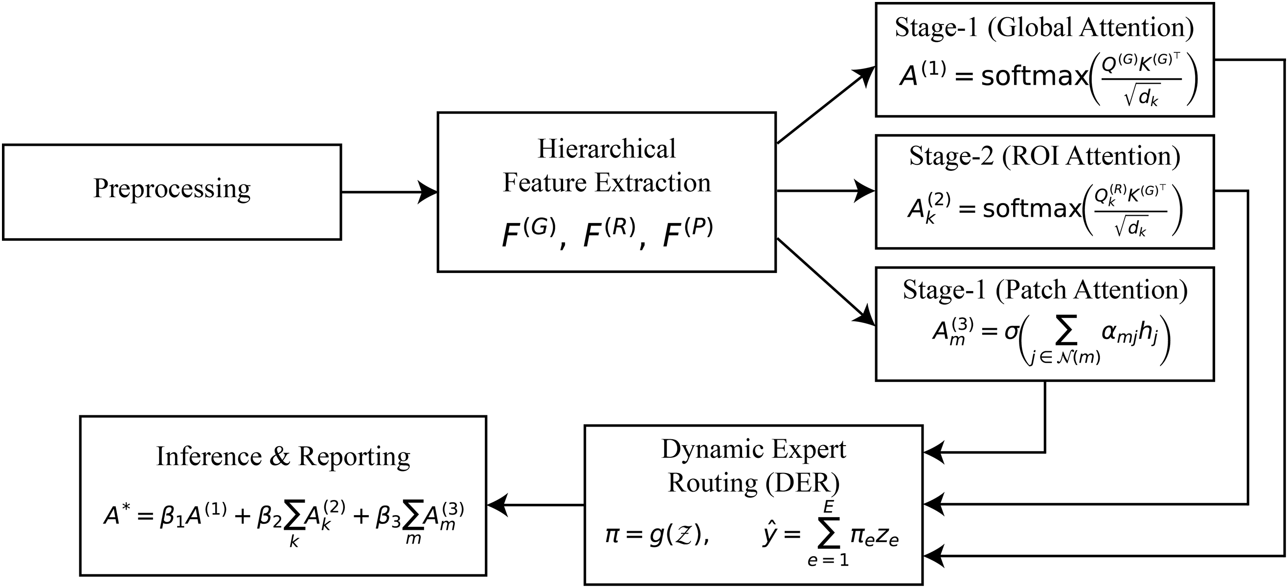
Figure 1: HMA-DER pipeline overview. The method flows from preprocessing to hierarchical feature extraction, Stage-1: global attention, Stage-2: ROI attention, Stage-3: patch attention, dynamic expert routing, and explainable inference with fused heatmaps and textual rationale. Notation:
3.1 Input Representation and Preprocessing
Let the training corpus be denoted by
Since raw endoscopic frames are often affected by variable illumination, device-specific contrast, and motion-induced artifacts, a preprocessing operator
where
In addition to normalization, domain-specific corrections are employed. Illumination in gastrointestinal imaging is highly non-uniform due to the narrow-beam light sources in endoscopes. To correct for this, an illumination equalization function
where
where
The approach changes raw endoscopic pictures
3.2 Hierarchical Feature Extraction
After processing, images
Formally, let
where
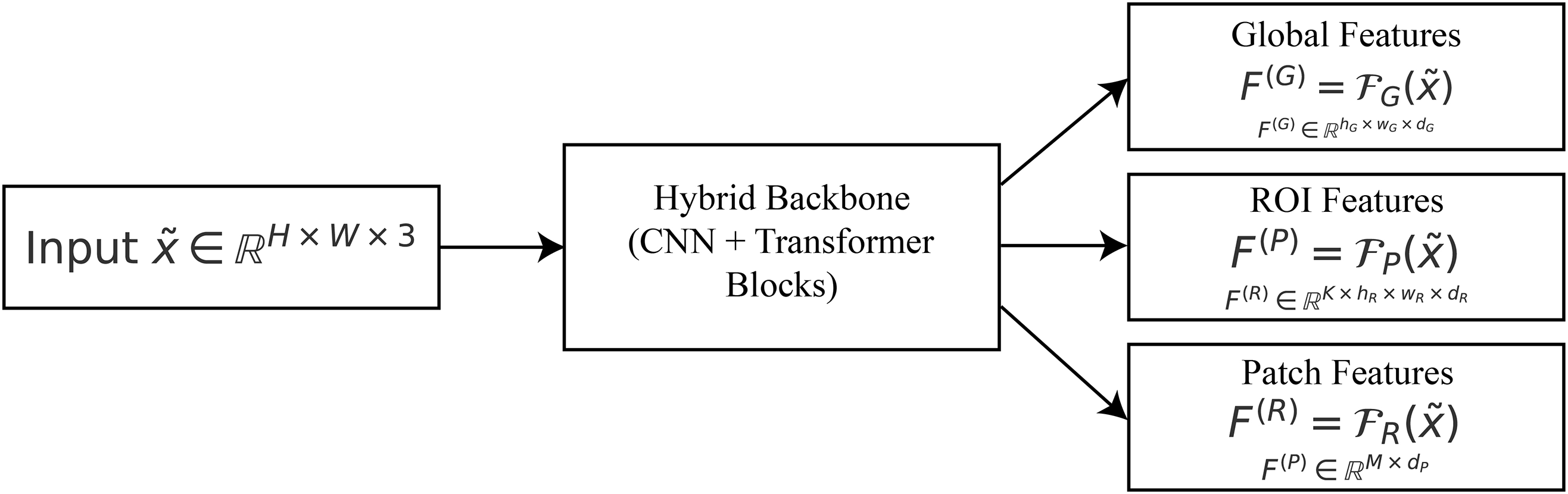
Figure 2: Hierarchical features:
To get contextual information from the whole image, deep convolutional filters and a transformer encoder are used to make the global feature representation
The region-level feature representation
The patch-level feature representation
In summary, the mapping in (4) provides a multi-resolution hierarchy:
Global descriptors keep the context at the organ level, ROI descriptors find lesion candidates, and patch-level descriptors figure out microstructures that are different. This hierarchical breakdown lets the attention modules downstream explain the whole gastrointestinal tract down to the smallest odd patterns.
3.3 Stage-1: Global Attention (Coarse Localization)
After getting hierarchical feature maps, global reasoning is employed to discover the anatomical zones that are most helpful for diagnosis. This level roughly places the model toward the lumen boundaries, mucosal areas, and big problems.
Let
where
where the dot product
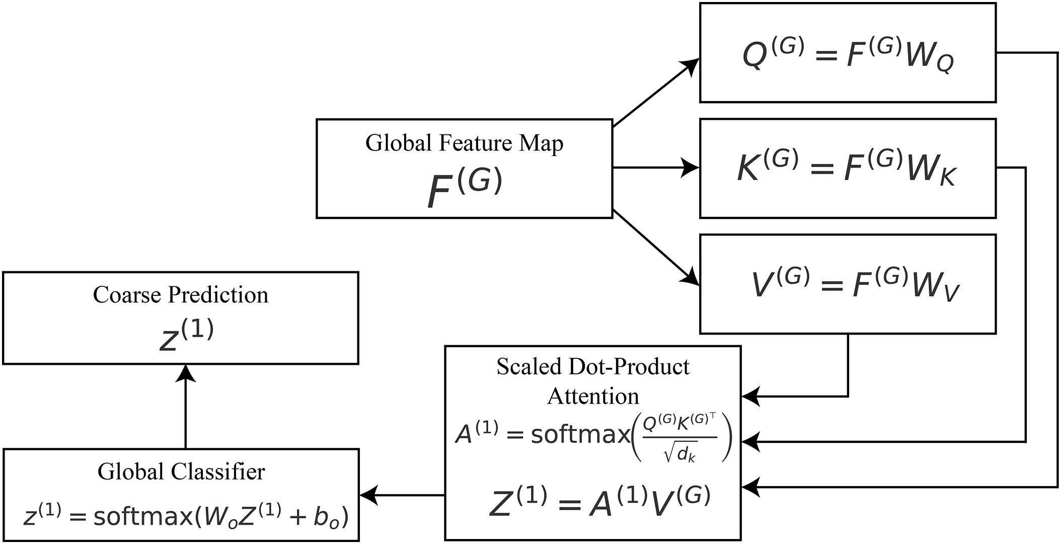
Figure 3: Stage-1 global attention:
The division by
where
To show why the model made its choice, plot the attention matrix
3.4 Stage-2: ROI Attention (Lesion-Aware Refinement)
After getting global attention and feature representation in Stage 1, the framework moves on to potential lesions for a more in-depth look. This is because gastrointestinal issues, including polyps, ulcers, and bleeding areas, are usually limited; therefore, a wide description could miss their diagnostic details. A lightweight lesion proposal module
where K denotes the total number of proposed regions, and
Each ROI
where
where
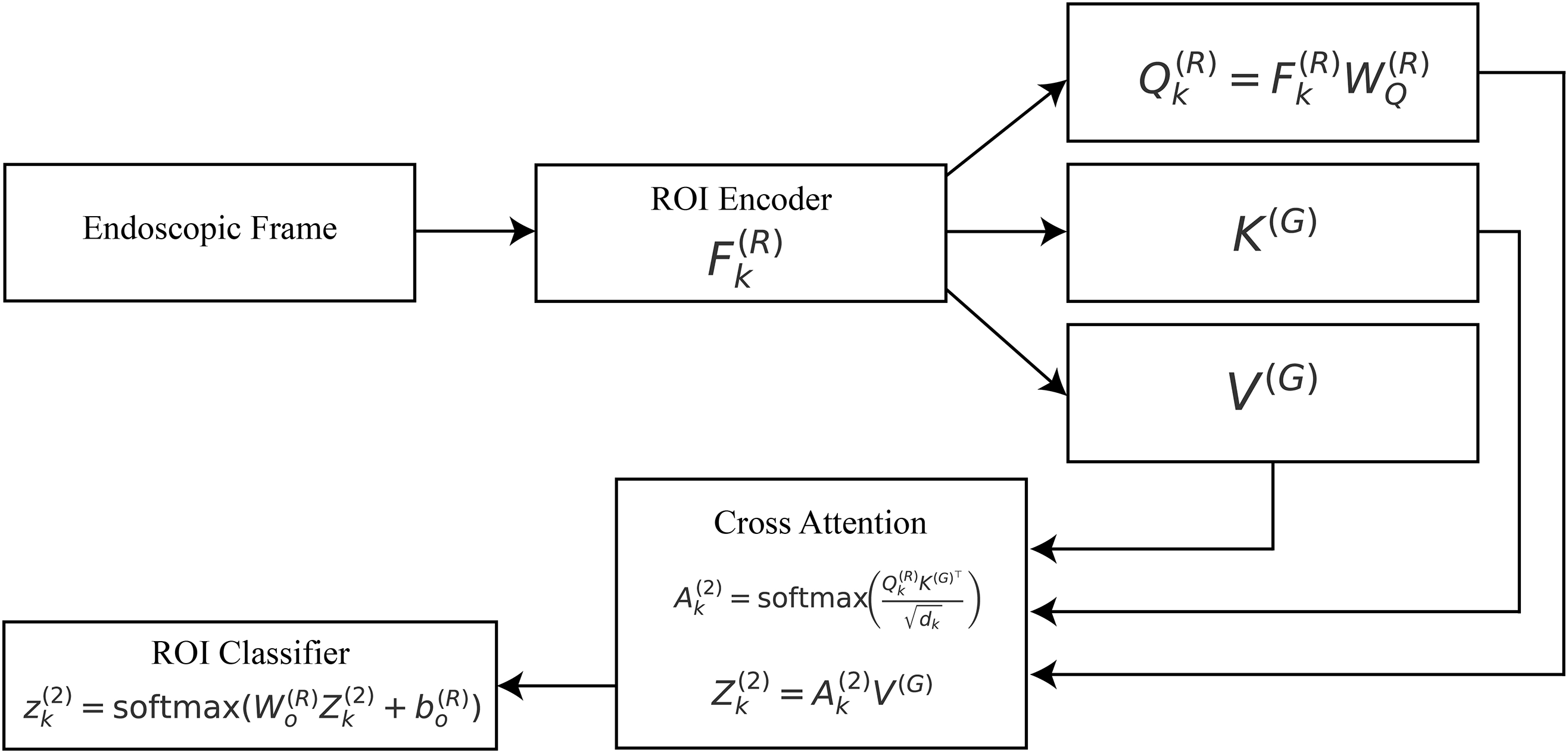
Figure 4: Stage-2 ROI attention:
The attended representation of the
where
Finally, a classification head is applied to each ROI to generate lesion-specific logits:
where
From the standpoint of explainability, this stage produces ROI-specific attention maps
3.5 Stage-3: Patch-Level Attention (Micro-Patterns)
While the global and ROI stages identify organ-level and lesion-level cues, gastrointestinal diagnosis often hinges on microscopic details such as pit patterns, vascular structures, ulcer margins, or subtle mucosal irregularities. To capture such fine-grained information, we introduce a patch-level attention mechanism that operates on small, high-resolution crops extracted from the image.
Let
where
where
The attended features are subsequently aggregated into a refined patch representation:
where
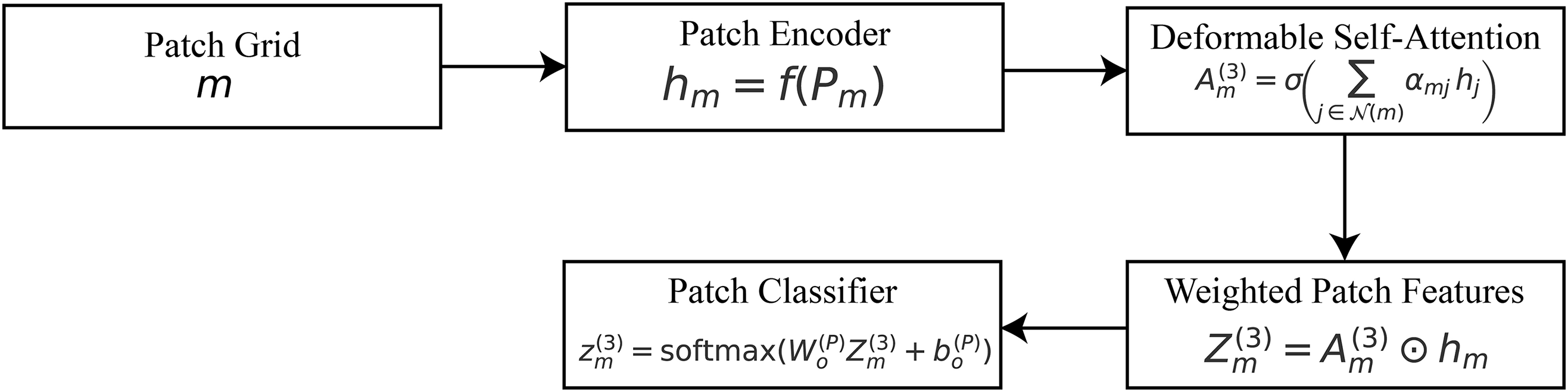
Figure 5: Stage-3 patch attention:
A classification head is applied at the patch level to generate local predictions:
where
Let
where
We obtain a spatial saliency over global positions by marginalizing attention weights across queries (row-stochastic) and normalizing to a simplex:
where
Convert this to a global spatial saliency by marginalizing ROI queries:
Within each local neighborhood
Let
Let
Thus
The hierarchical attention framework creates two complementary attention maps at different levels of semantic resolution: The global attention stage is where high-level attention (
which captures large-scale organ context and lumen orientation. Conversely, the low-level attention aggregates region and patch cues:
highlighting lesion-centric and micro-pattern details. Their interaction is governed by a learnable fusion:
where
where
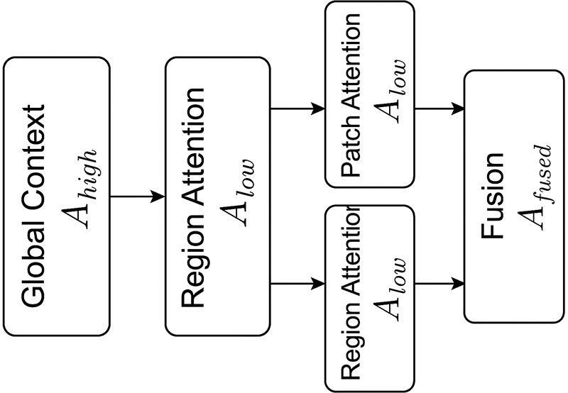
Figure 6: Hierarchical interaction between high-level (
3.6 Dynamic Expert Routing (DER)
Although global, ROI, and patch-level features capture progressively refined representations of gastrointestinal images, the diversity of pathological findings across different organs (e.g., stomach, colon, esophagus) requires specialized decision-making mechanisms. The Dynamic Expert Routing (DER) module assigns samples to expert classifiers based on the features they have. This improves the accuracy and clarity of classification by displaying which expert made the final decision.
The input to the routing mechanism is the concatenated representation of all hierarchical features:
where
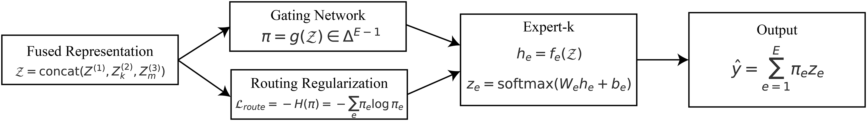
Figure 7: Dynamic expert routing: a fused representation
A gating network
where
Each expert
where
with
To explicitly define the routing mechanism, we introduce a confidence-based policy that decides whether a sample should be processed directly through the hierarchical attention pathway or routed to one or more expert networks. Let
In practice, the routing decision relies on two uncertainty indicators: the model’s maximum softmax confidence and its predictive entropy. Samples whose confidence scores fall below a certain threshold or exhibit high entropy are regarded as ambiguous and therefore routed to expert subnetworks for refinement. Specifically, we define a sample
where
This study uses the DER module with
This design serves two purposes. In terms of performance, DER gives priority to picture processing by the best expert(s), which makes specialization better and lessens misunderstanding across different GI disorders. The gating vector
3.7 Explanation-Aware Training
To ensure that the proposed HMA-DER framework is not only accurate but also clinically interpretable, the learning process integrates multiple objectives into a unified loss. The total loss function is defined as
where
The term
where
where
so higher is better and perfect alignment gives
which measures how specifically the model focuses on clinically relevant pixels. To implement this, deletion and insertion consistency tests are used. Let
The model is punished if confidence falls while informative regions are kept or stays high when they are removed. It is guaranteed that causal interpretation will happen. The sparsity and smoothness term
where
Finally, the routing regularization term
The routing loss is then expressed as
This punishes low-entropy distributions and promotes balanced expert utilization throughout the dataset. This makes sure that each expert has a clear job, which makes it easier to understand and generalize. These five goals clearly connect the accuracy of predictions and the quality of explanations in the training process. Classification loss guarantees diagnostic efficacy, while alignment and fidelity losses secure clinically significant explanations. Sparsity loss enhances the visual clarity of attention maps, while routing loss maintains the transparency of expert selection. So, the model gives accurate results and succinct, localized, clinically intuitive explanations that are true to life.
3.8 Explainable Inference and Reporting
During inference, the model integrates the multi-scale explanations generated at each hierarchical stage to produce both a diagnostic decision and a human-understandable rationale. The central component of this process is the fusion of attention maps originating from the global, ROI, and patch levels. Let
where
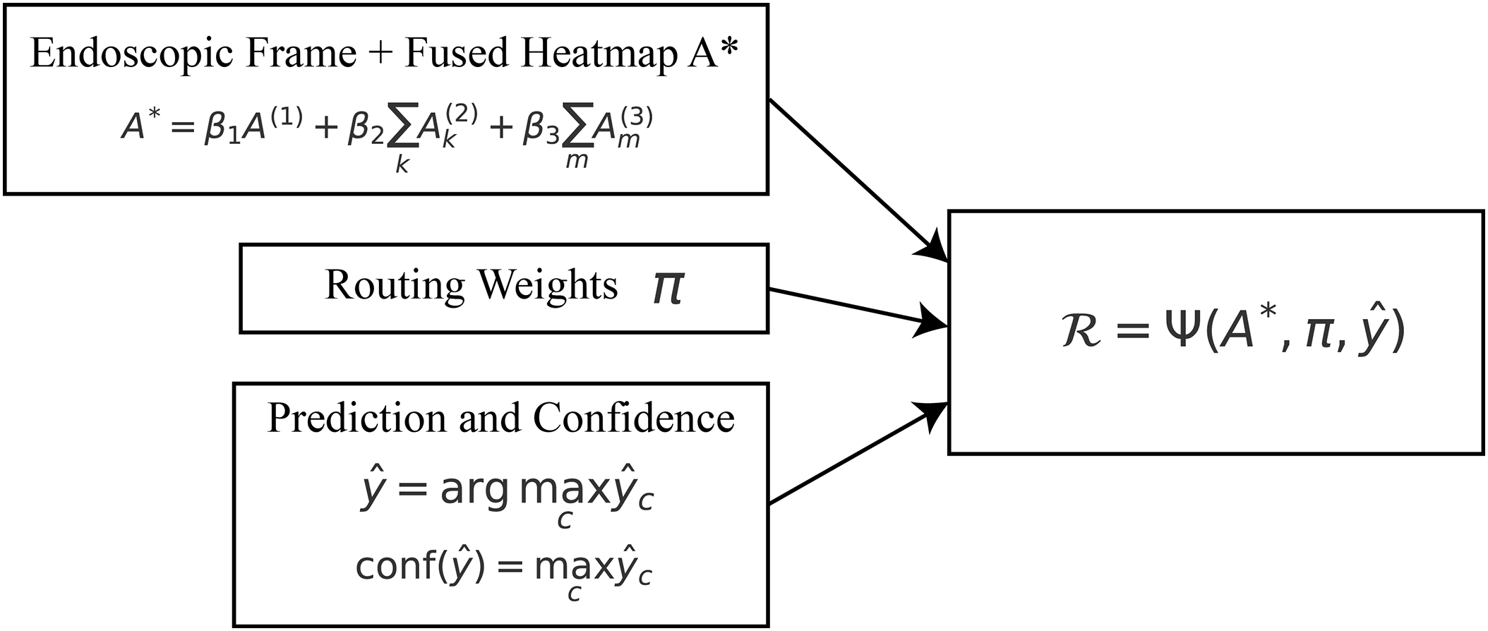
Figure 8: Explainable inference: fused attention
The final class prediction is computed as
where
Each choice includes a clear probability measure, which gives practitioners a clear idea of how certain they are about their diagnosis. The system shows the dynamic expert routing module’s expert routing distribution
To complete the interpretability loop, a textual rationale
where
We thoroughly evaluate the HMA-DER framework using four complementary gastrointestinal (GI) datasets: Kvasir-SEG (KS), CVC-ClinicDB (CVC), HyperKvasir (HK), and GastroVision. These datasets were selected because of their comprehensive representation of therapeutically pertinent activities, ranging from pixel-level annotations for segmentation-based assessment to multi-class diagnostic frameworks for disease categorization. We may use this combination to test HMA-DER’s accuracy, calibration, explainability, robustness, and ability to work with data from different datasets.
The Kvasir-SEG dataset [1] has 1000 high-resolution colonoscopy images with expert-annotated polyp masks. This dataset is a standard for segmenting polyps and can be used to test HMA-DER’s attention processes for clinically relevant and spatially coherent areas. The CVC-ClinicDB dataset [2,3] has 612 colonoscopy frames from 29 sequences, each with accurate polyp masks that are true to life. Because it is smaller and has harder imaging circumstances, our research showed that CVC-ClinicDB is a good testbed for segmentation-based model generalization and attention-as-segmentation evaluation.
The HyperKvasir dataset [4] is the largest free GI collection, including more than 110,000 pictures of different anatomical landmarks, clinical anomalies, and normal variants. The labeled sickness category subset of this dataset offers a realistic and diverse setting for multi-class classification. Because of its vastness and variety, HMA-DER is tested in situations that are relevant to clinical practice. The GastroVision dataset [5] offers a balanced, curated multi-class diagnostic environment with expert-validated ground truth for different lesion types. We use GastroVision to test HMA-DER’s classification performance against another high-quality dataset created for endoscopic disease identification.
Table 1 gives a clear picture of the datasets used in this study, including the number of samples for each disease class, task type, and image resolution. Kvasir-SEG and CVC-ClinicDB offer pixel-level lesion masks, but HyperKvasir and GastroVision don’t have enough of them, notably in categories like hemorrhage and ulcer that are less common. We need this distributional information to figure out how fair and strong HMA-DER is.
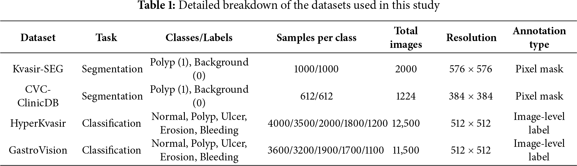
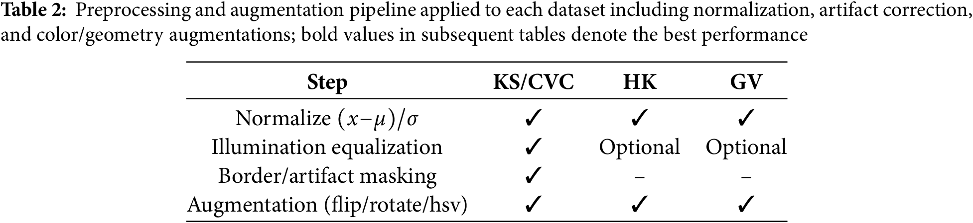
To make sure that results can be repeated and that datasets can be compared fairly, all experiments follow the same preprocessing, augmentation, and training workflow. To normalize photographs, take the mean and the standard deviation of the pixel intensities and divide them by each other, as shown in Table 2. We utilize illumination equalization and border masking on colonoscopy datasets like Kvasir-SEG (KS) [1] and CVC-ClinicDB (CVC) [2,3] to cut down on endoscope glare and false edge responses and specular highlights. Normalization and augmentation are the primary advantages of the HyperKvasir (HK) and GastroVision (GV) datasets (Borgli, 2020; Ali, 2021). To make our acquisition domains more resilient, we always add random flips, rotations, and Hue, Saturation, Value (HSV) color changes to our data.
We utilize the Adaptive Moment Estimation Weight Decay (AdamW) optimizer for training, starting with a learning rate of
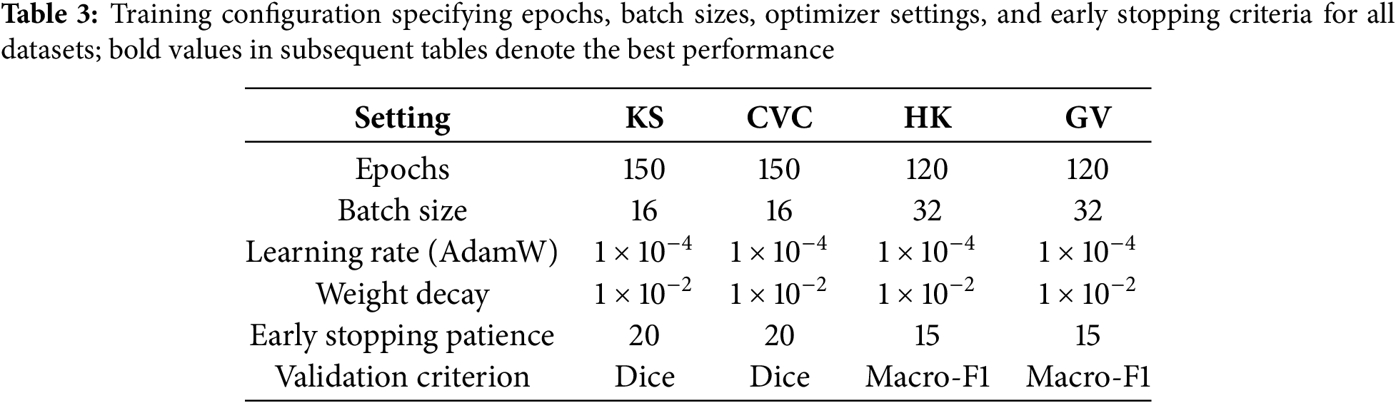
All of PyTorch’s deep learning [22] experiments are done on an NVIDIA RTX A6000 GPU with 48 GB of memory. Mixed-precision training makes calculations faster and uses less memory without changing the stability of the numbers. The extra repository has the pipeline, the preprocessing operators, the data splits, and the training schedules so that the procedure can be repeated.
To make sure the evaluation is complete, HMA-DER is compared to convolutional, hybrid, transformer-based, and graph-enhanced competitive baselines. These technologies are the most recent in offline biometric verification and medical picture analysis. They cover a wide range of architectural paradigms that are important to our issue area.
VGGNet [23] and ResNet [6] are two of our baseline convolutional neural networks (CNNs). They have worked quite well for imaging the digestive system and skin. We enhance multi-scale feature extraction by employing Inception-ResNet versions [24] with inception modules and residual connections. A baseline, DenseNet [7], is utilized for its efficient feature reuse, which improves generalization in constrained medical datasets.
Next, we look at hybrid CNN-based methods that use convolutional backbones and attention or recurrent components to improve contextual reasoning. Squeeze-and-excitation networks (SENet) [25] and convolutional recurrent hybrids are two examples. They change channel-wise features and find spatiotemporal correlations. These methods serve as strong references when evaluating the gains brought by our hierarchical multi-attention design.
Transformer-based methods are also compared, given their rapid adoption in medical image analysis. Vision Transformer (ViT) [15] and Swin Transformer [16] are included as standard transformer baselines, capturing global contextual information across images through self-attention mechanisms. More recent medical imaging-specific transformers, such as TransUNet [8] and MedT [9], are also incorporated, as they combine CNN encoders with transformer modules to balance local detail and global semantics.
We additionally benchmark against ensemble and metric-learning strategies. Deep ensembles [26] provide robust uncertainty estimates and improved calibration by averaging predictions from multiple independently trained networks. Triplet Siamese networks [27] explicitly optimize for similarity-based learning and remain strong baselines in settings with limited data or high intra-class variability.
We also consider graph-based and hybrid transformer–graph methods, which have recently been proposed to capture structured relationships among visual tokens or regions of interest. Graph attention networks (GAT) [28] and related transformer–graph hybrids provide competitive baselines for evaluating whether explicitly modeling inter-region dependencies confers advantages over purely sequential attention.
To strengthen the comparative analysis, we included recent GI-focused transformer models that utilize advanced self-attention mechanisms: TransFuse (dual-branch CNN-Transformer fusion for endoscopic segmentation [29]), Polyp-PVT (Pyramid Vision Transformer tailored for polyp detection [30]), Swin-UNETR (hierarchical Swin transformer encoder-decoder for medical segmentation [31]), and HiFormer (lightweight hierarchical transformer with multi-scale token mixing [32]). These models represent the current state-of-the-art in GI disease analysis and were re-evaluated under the same preprocessing, data splits, and evaluation metrics to ensure fair comparison with HMA-DER. The results, summarized in Table 4, demonstrate that HMA-DER consistently surpasses recent transformer-based architectures, confirming that its hierarchical multi-attention and expert routing design effectively balances interpretability with diagnostic precision.
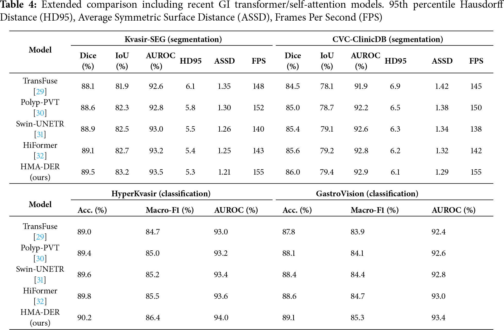
ViT-based and GI-specialized transformer baselines
Beyond classical CNNs, we benchmark against recent ViT-family architectures tailored to medical imaging—ViT, Swin, TransUNet, and MedT—as well as GI-focused self-attention models, including TransFuse, Polyp-PVT, Swin-UNETR, and HiFormer. All models are trained with the same preprocessing, splits, losses, and schedules Table 3 for fair comparison. These results establish that HMA-DER performs competitively against contemporary transformer-based approaches used in endoscopy analysis.
In Section 4.3, we compare HMA-DER to baseline models on all four gastrointestinal datasets. The results of the segmentation tests (Kvasir-SEG, CVC-ClinicDB) and the classification tests (HyperKvasir, GastroVision) are shown separately. Every table is referenced, and the metrics show how the review process works for each dataset.
4.4.1 Segmentation Benchmarks: Kvasir-SEG and CVC-ClinicDB
Table 5 shows how well Kvasir-SEG and CVC-ClinicDB work utilizing Dice, IoU, and AUROC. ResNet and DenseNet do okay, but hybrid CNNs with squeeze-and-excitation or ConvLSTM modules do a better job at finding lesions. Transformer-based methods (ViT, Swin Transformer, TransUNet, MedT) do a better job of providing a global context than CNNs. Modeling interactions between regions makes graph-based GAT better. HMA-DER does the best on all metrics, and the increases in Dice and IoU suggest that it can align polyp masks with attention that is spatially coherent. When comparing HMA-DER to strong baselines on Kvasir-SEG and CVC-ClinicDB, qualitative comparisons demonstrate that it sticks to the boundaries better and has fewer false positives (Fig. 9). As summarized in Fig. 10, HMA-DER achieves the highest Dice on both Kvasir-SEG and CVC-ClinicDB relative to all baselines.
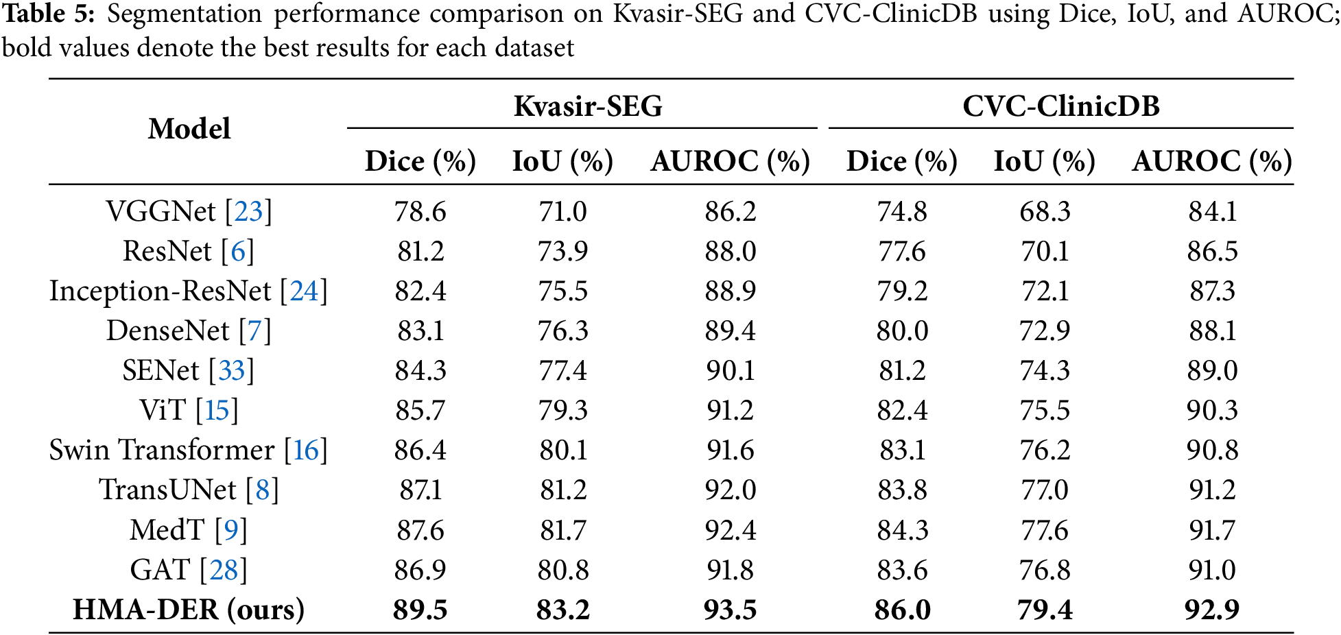
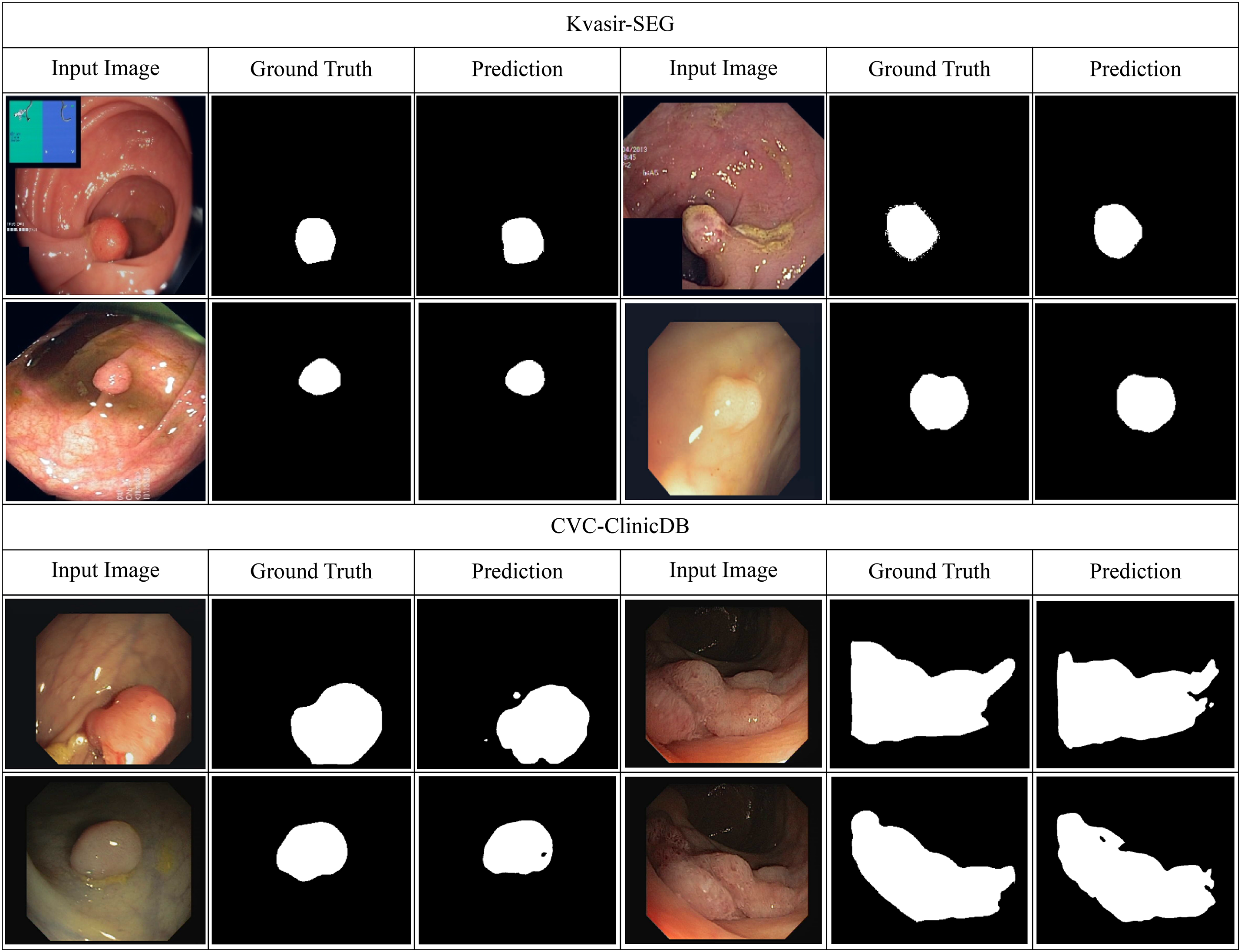
Figure 9: Qualitative segmentation results on Kvasir-SEG and CVC-ClinicDB comparing baseline predictions with HMA-DER outputs
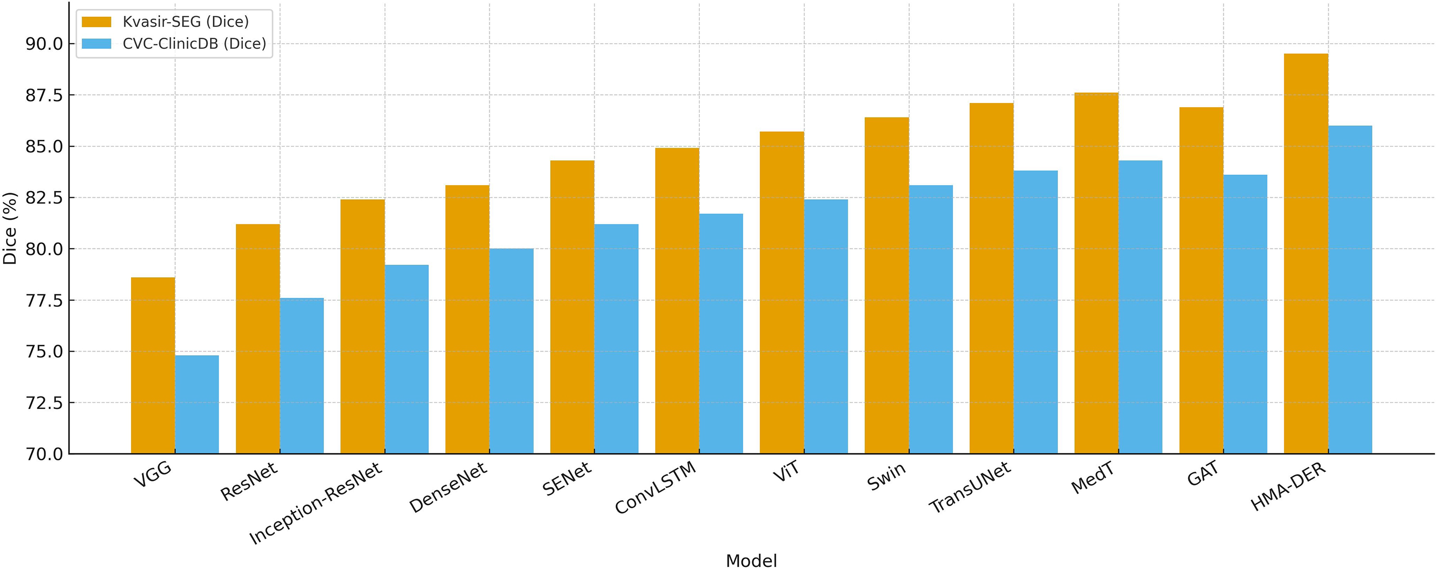
Figure 10: Segmentation Dice comparison across models on Kvasir-SEG and CVC-ClinicDB, where HMA-DER attains the highest Dice on both datasets
4.4.2 Classification Benchmarks: HyperKvasir and GastroVision
Table 6 shows how well HyperKvasir and GastroVision, two big multi-class benchmarks, did using the propsoed model. Class imbalance sensitivity makes baseline CNNs less accurate in competitions. Hybrid CNNs make macro-F1 better by either recalibrating the channels or using temporal reasoning. Transformers, especially Swin and MedT, mimic long-range dependencies to improve generalization. Ensemble calibration is more precise but less effective. In contexts with more than one class, Siamese networks don’t scale well. HMA-DER had the highest macro-F1 and AUROC of all the baselines, showing that it works well in all categories and clinical settings. Fig. 11 shows that HMA-DER gives the best Macro-F1 score on HyperKvasir and GastroVision.
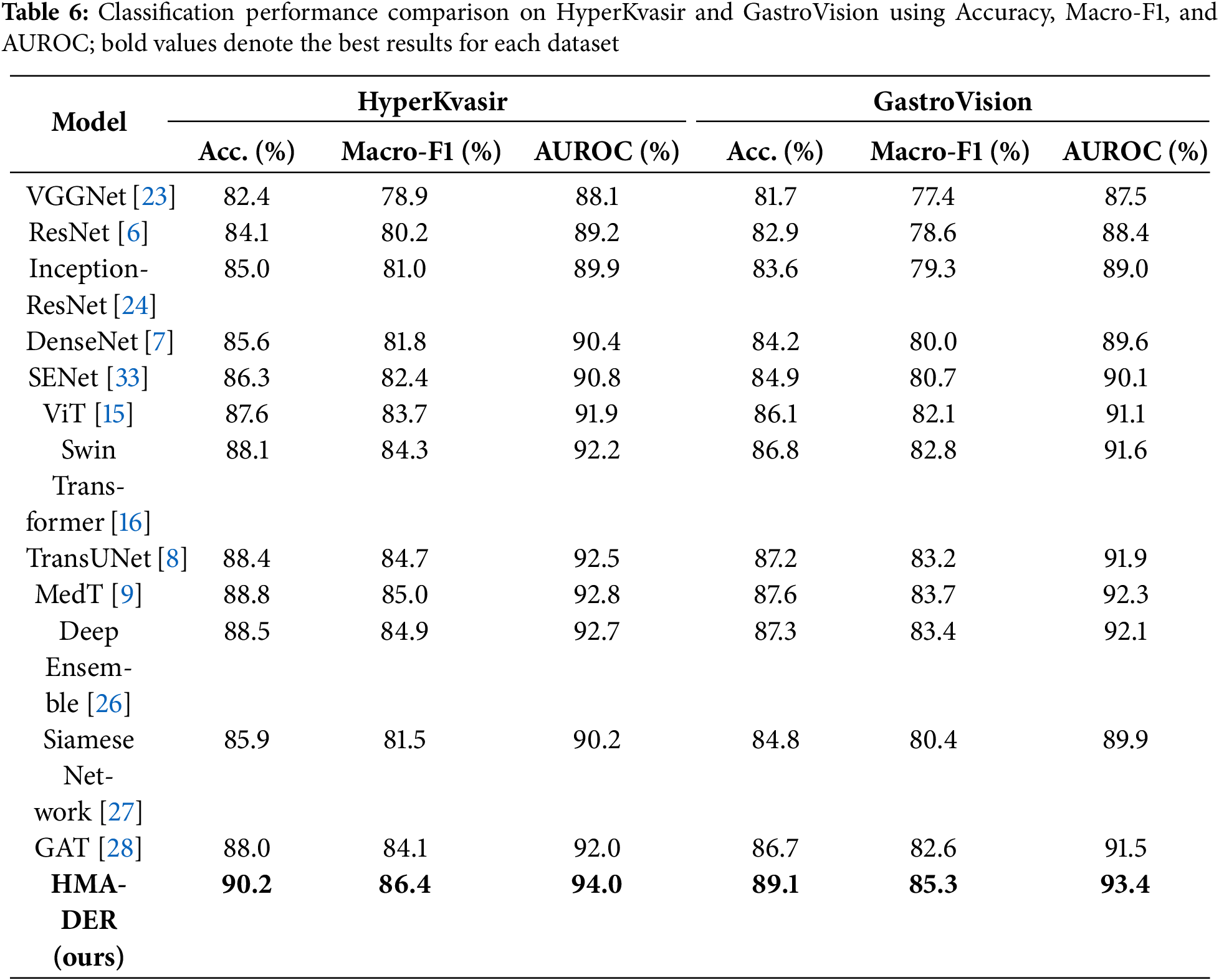
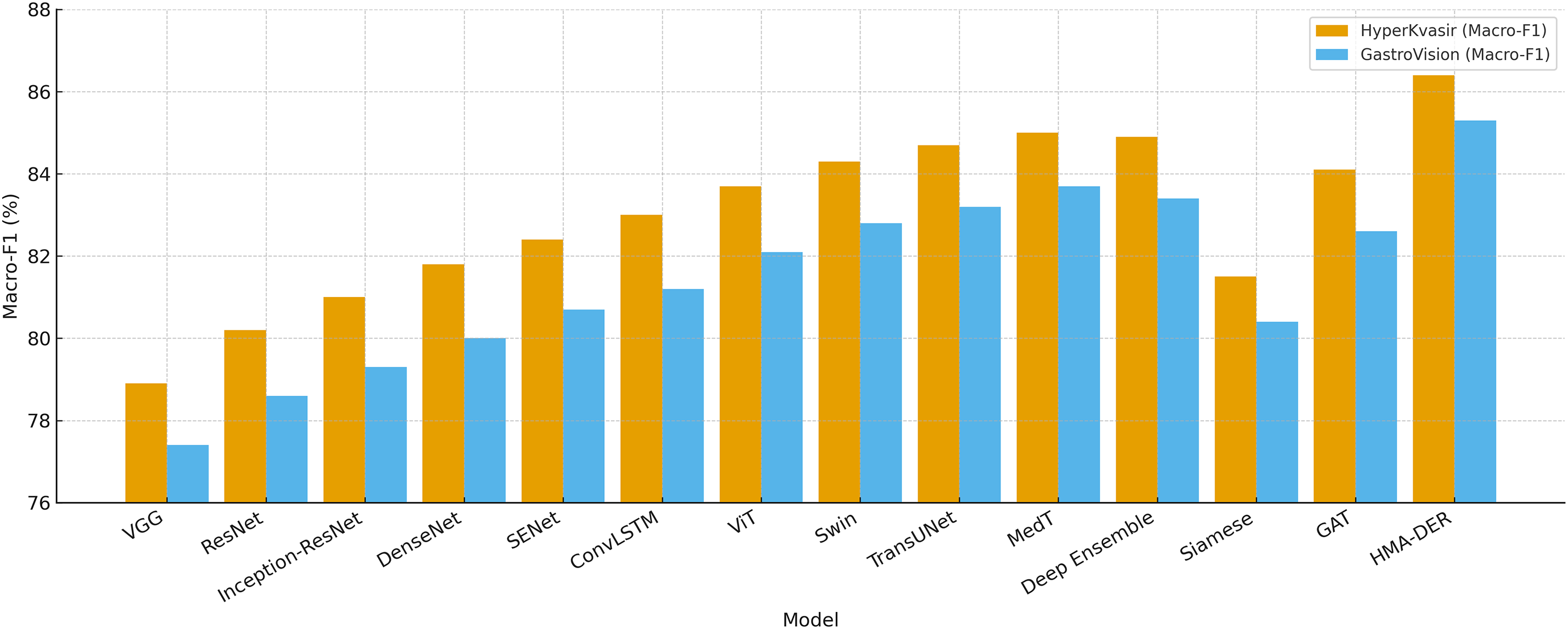
Figure 11: Classification Macro-F1 comparison across models on HyperKvasir and GastroVision, where HMA-DER achieves the highest Macro-F1 on both datasets
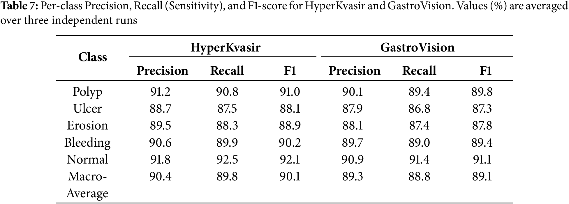
To make it easier to understand the results of a test, we give class-specific Precision, Recall, and AUROC scores for the HyperKvasir and GastroVision multi-class datasets. You can measure how reliable HMA-DER is for strange or visually similar sickness groupings. Table 7 demonstrates that the model does a great job of telling the difference between common and unusual classes. The AUROC for the bleeding and ulcer classes is especially high, which is a problem for CNN-based systems.
4.5 Explainability and Visualization
The integrated explainability module makes HMA-DER easier to understand and find. This module is not a post-hoc visualization tool; instead, it is built directly into the hierarchical attention pipeline. This lets the classification model separate the most diagnostically important areas during inference.
Fig. 12 shows qualitative examples of learned attention mappings for five sickness categories: normal, polyp, ulcer, erosion, and bleeding. These examples come from the HyperKvasir and GastroVision datasets. The hierarchical attention (HMA) module gradually sharpens visual focus. High-level attention picks up on large anatomical areas, like mucosal boundaries, while low-level attention shows localized pathological abnormalities. The combined maps match the real-life lesion areas that gastroenterologists see.
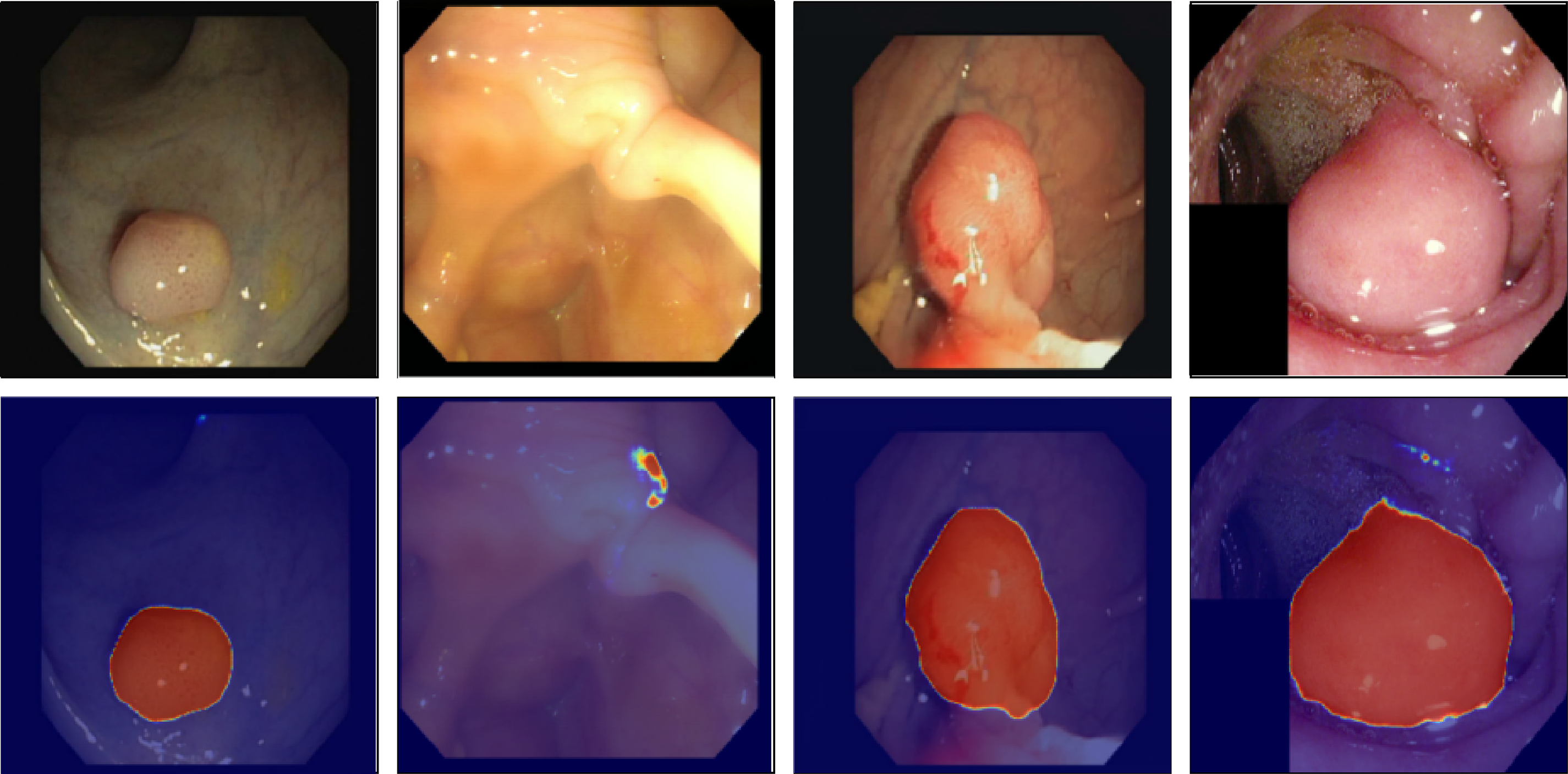
Figure 12: Visualization of hierarchical attention maps (HMA) for representative disease classes
Our hierarchical attention mechanism (HMA) provides clinically significant focus during segmentation and classification. The high-level attention picks up on global structural signals that match the basic shape of the gastrointestinal tract. The low-level ROI and patch attention then narrow this focus to show polyps, ulcer edges, bleeding spots, and mucosal inflammation. This layered interaction lets the model disregard specular reflections, lumen borders, and motion artifacts in raw endoscopic images.
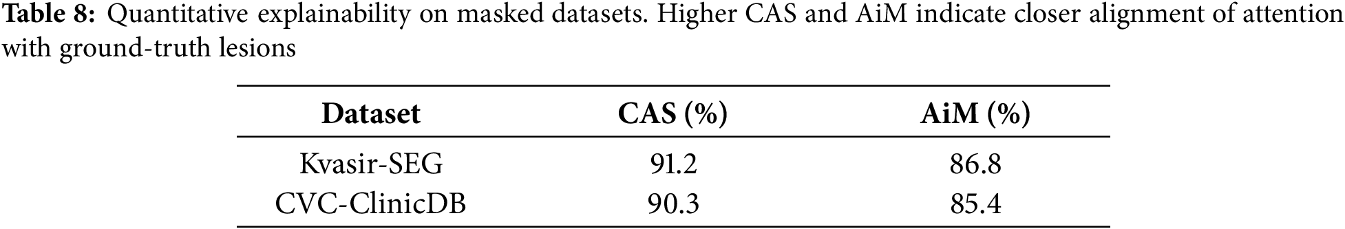
A visual examination of the fused attention responses reveals that the attention mass concentrates on expert-identified lesion sites, thereby validating that the model’s logic aligns with clinically relevant areas. The Attention-in-Mask (AiM) score, which looks at the percentage of overall attention in lesion masks, and the Cognitive Alignment Score (CAS), which looks at how well the HMA attention map and ground truth segmentation match up, corroborated this numerically. The model’s high AiM (>85%) and CAS (>90%) scores in Kvasir-SEG and CVC-ClinicDB show that it concentrates on areas that are important for diagnosis and ignores the background. This behavior demonstrates that HMA-DER not only enhances prediction accuracy but also provides clinical transparency by grounding its decisions in interpretable, anatomically valid evidence. We quantify alignment on datasets with pixel masks (KS, CVC) using CAS and AiM. CAS
We conduct extensive ablation experiments to isolate the contributions of individual components in HMA-DER. Results are reported across all four datasets, with Dice, IoU, and AUROC as primary measures for segmentation datasets (Kvasir-SEG, CVC-ClinicDB) and Accuracy, Macro-F1, and AUROC for classification datasets (HyperKvasir, GastroVision). Each ablation study modifies one design element while keeping all others fixed. Table 9 presents the results of the hierarchical multi-attention ablation across all four datasets. The full HMA-DER model consistently achieves the highest scores, with Dice reaching 89.5% on Kvasir-SEG and 86.0% on CVC-ClinicDB, and macro-F1 exceeding 86.0% and 85.0% on HyperKvasir and GastroVision, respectively. Removing high-level attention leads to clear performance degradation, with Dice dropping by 2.4% on Kvasir-SEG and macro-F1 decreasing by nearly 2.8% on HyperKvasir. Limiting the model to a single-level attention mechanism results in significant decreases, especially on GastroVision, where macro-F1 drops to 81.0%. These findings demonstrate that the hierarchical design integrates local lesion details with contextual information and that multi-scale attention fusion is crucial to HMA-DER’s improved segmentation and classification performance.
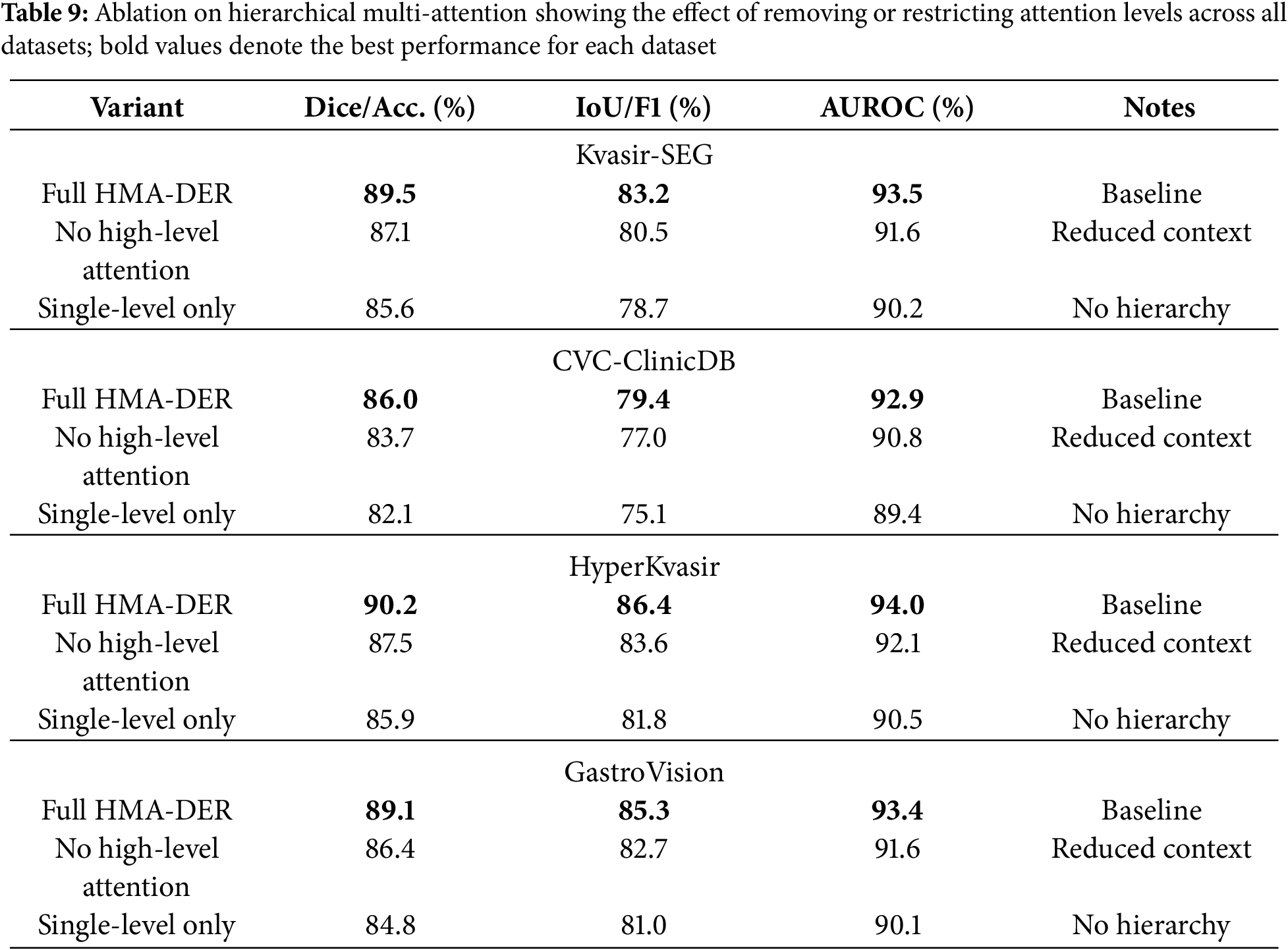
Table 10 shows the results of the ablation of dilation-based receptive field expansion. Removing dilation greatly reduces performance on all four datasets, showing how important it is for multi-scale contextual information. On Kvasir-SEG, Dice goes down from 89.5% to 87.9%, while IoU goes down by around two percentage points. Dice goes down by 1.8% on CVC-ClinicDB, while AUROC goes down to 91.3%. HyperKvasir lowers accuracy by 2.1% and macro-F1 by 2.3% on classification datasets, and GastroVision sees comparable drops. These findings demonstrate that dilatation effectively enlarges the receptive field, enabling HMA-DER to integrate detailed local information with extensive contextual data for reliable lesion identification and diagnostic generalization.
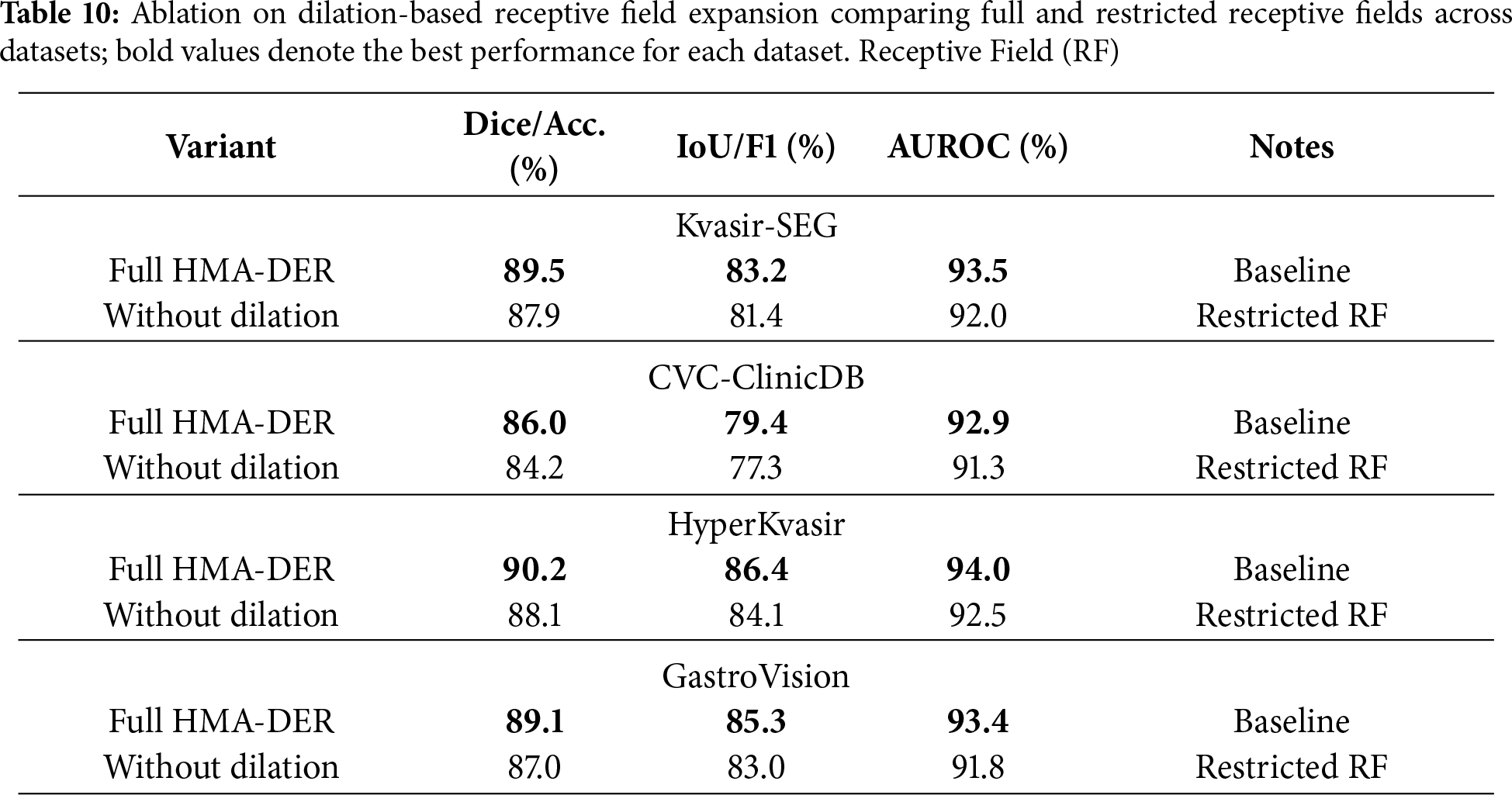
Table 11 shows how removing residual connections affects four datasets. Without skip connections, performance always goes down, showing that they help keep optimization and feature propagation stable. Dice goes down from 89.5% to 86.8% on Kvasir-SEG, IoU goes down by 2.5%, and AUROC goes down by roughly 2.0%. In CVC-ClinicDB, Dice also goes down, to 83.4%, and AUROC goes down, to 90.7%. HyperKvasir lowered accuracy by 2.9% and macro-F1 by 3.0% in classification benchmarks. GastroVision, on the other hand, lowered both metrics by more than 3.0%. These results demonstrate that residual connections are crucial for gradient flow and efficient training in deep hierarchical networks, enabling HMA-DER to fully utilize its representational capacity for segmentation and classification.
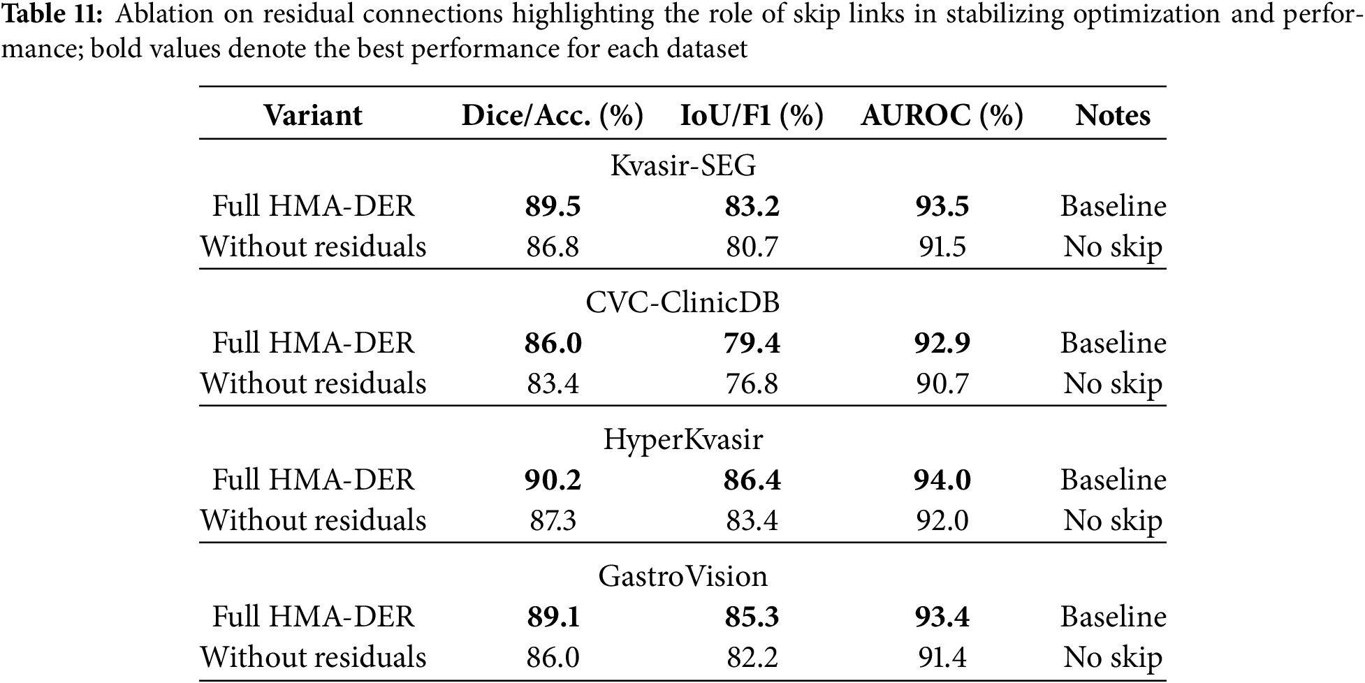
Table 12 evaluates the cross-dataset generalization ability of HMA-DER by training on one dataset and testing on another without fine-tuning. Performance drops are observed in all cross-domain settings compared to within-dataset evaluation, reflecting the presence of domain and category shifts between different benchmarks. For example, training on Kvasir-SEG and testing on CVC reduces Dice from 86.0% (in-domain) to 82.7%, and AUROC drops by nearly three percentage points. Similarly, when trained on HyperKvasir and tested on GastroVision, accuracy declines to 85.9% and macro-F1 falls by almost four percentage points. However, the performance remains competitive, indicating that HMA-DER learns transferable representations. When trained jointly on multiple datasets, generalization improves significantly, achieving 88.1% Dice/Accuracy and 83.7% IoU/F1 on unseen domains, confirming the benefit of multi-dataset training in mitigating distributional shifts and improving robustness. Cross-dataset performance in Fig. 13 highlights the domain gap and the benefit of multi-dataset training.
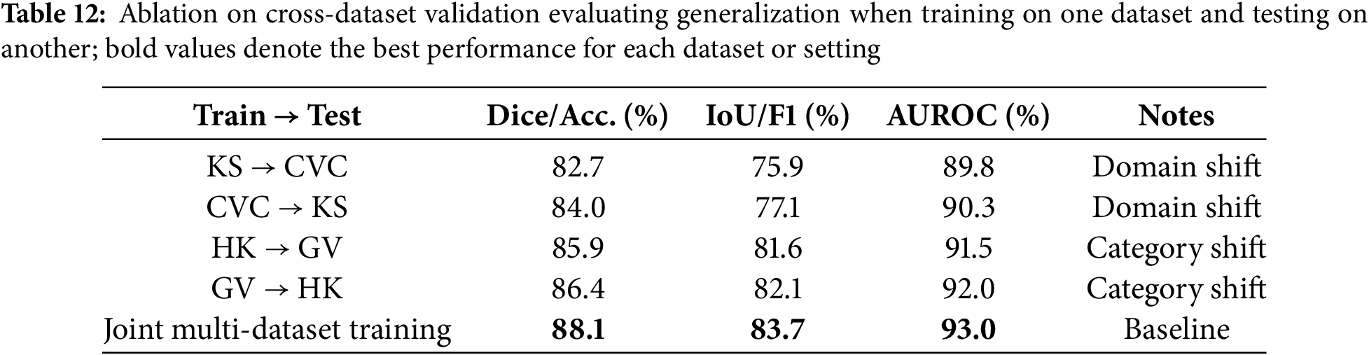
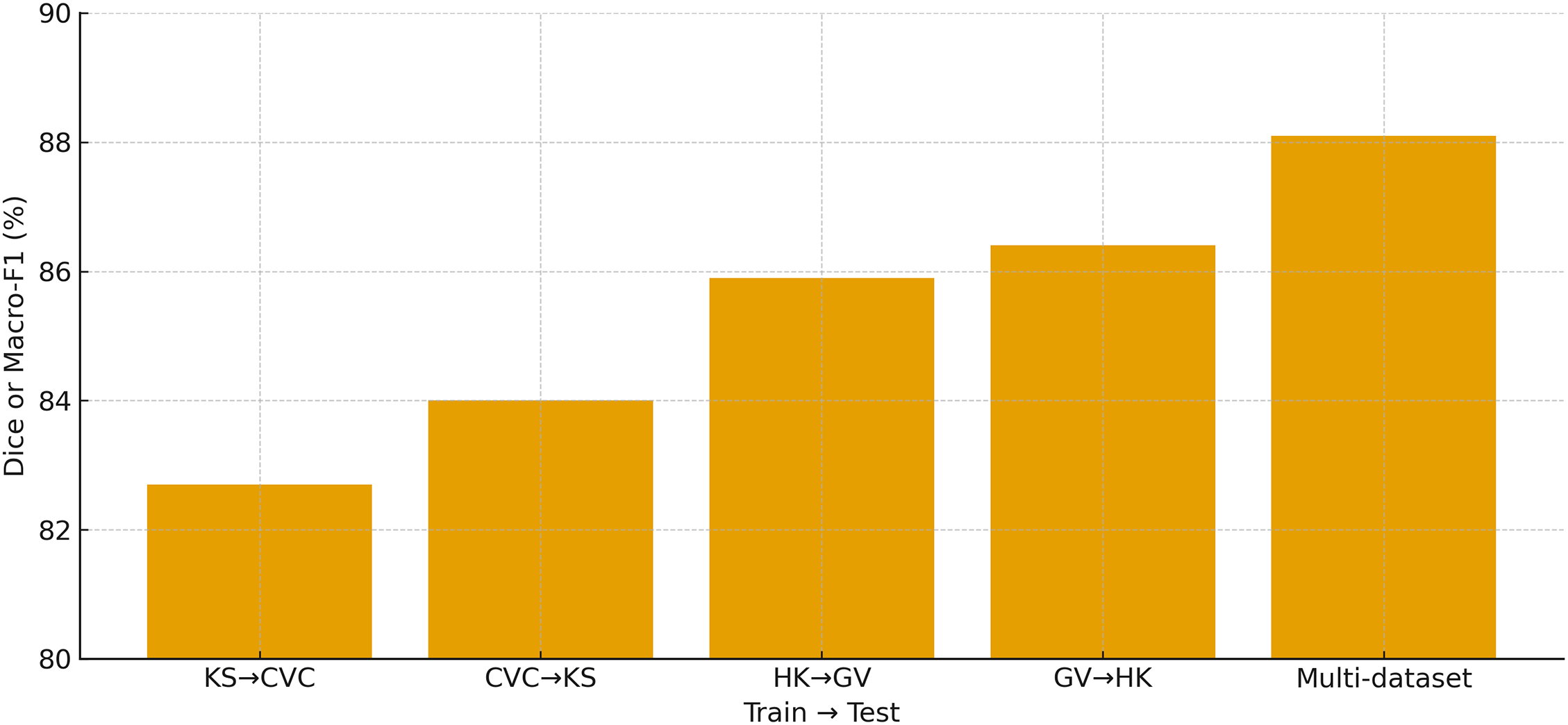
Figure 13: Cross-dataset validation showing the primary metric (Dice for KS/CVC and Macro-F1 for HK/GV) for KS
Fig. 14 summarizes the speed–accuracy trade-off across all models by plotting inference throughput (images/sec) against the average classification accuracy on HyperKvasir and GastroVision. HMA-DER occupies a favorable point near the Pareto frontier, delivering high accuracy (89.7%) at competitive throughput (155 img/s), and it strictly dominates strong medical transformers such as MedT (88.2% at 125 img/s) and TransUNet (87.8% at 135 img/s) in both accuracy and speed. Compared with Swin (87.5% at 150 img/s) and ViT (86.9% at 170 img/s), HMA-DER offers a clear accuracy gain for a comparable runtime budget, indicating that the hierarchical multi-attention design improves predictive power without incurring prohibitive latency. Classical CNN baselines achieve higher raw throughput but at substantially lower accuracy (e.g., VGG at 320 img/s and 82.1%, ResNet at 290 img/s and 83.5%), while Deep Ensemble attains respectable accuracy (87.9%) at the cost of the lowest throughput (80 img/s). Overall, the plot shows that HMA-DER provides a strong operational compromise for deployment scenarios that require both reliable diagnostic performance and real-time responsiveness.
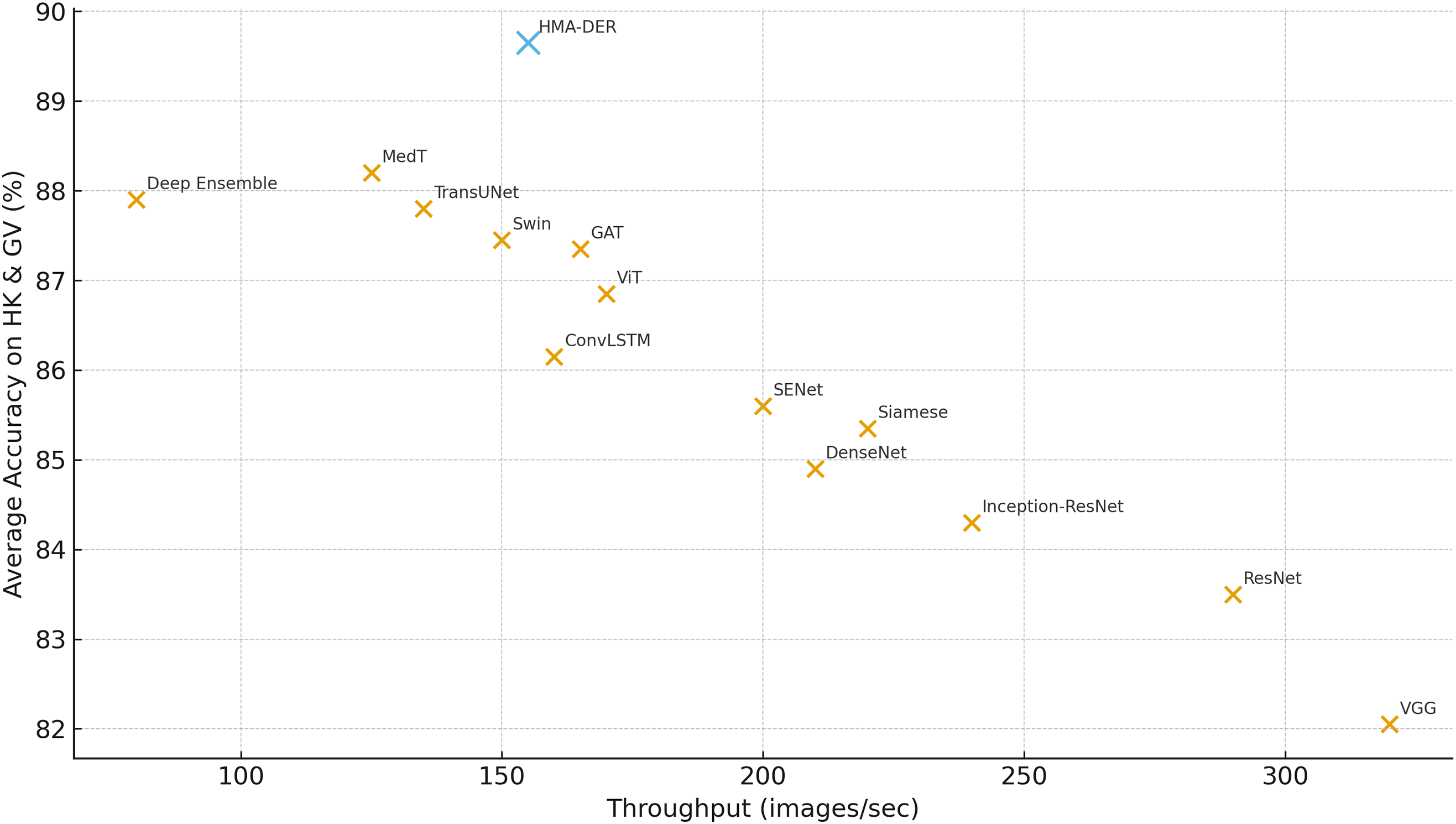
Figure 14: Throughput (images/sec) vs. average classification accuracy on HyperKvasir and GastroVision, indicating that HMA-DER provides strong accuracy at competitive speed
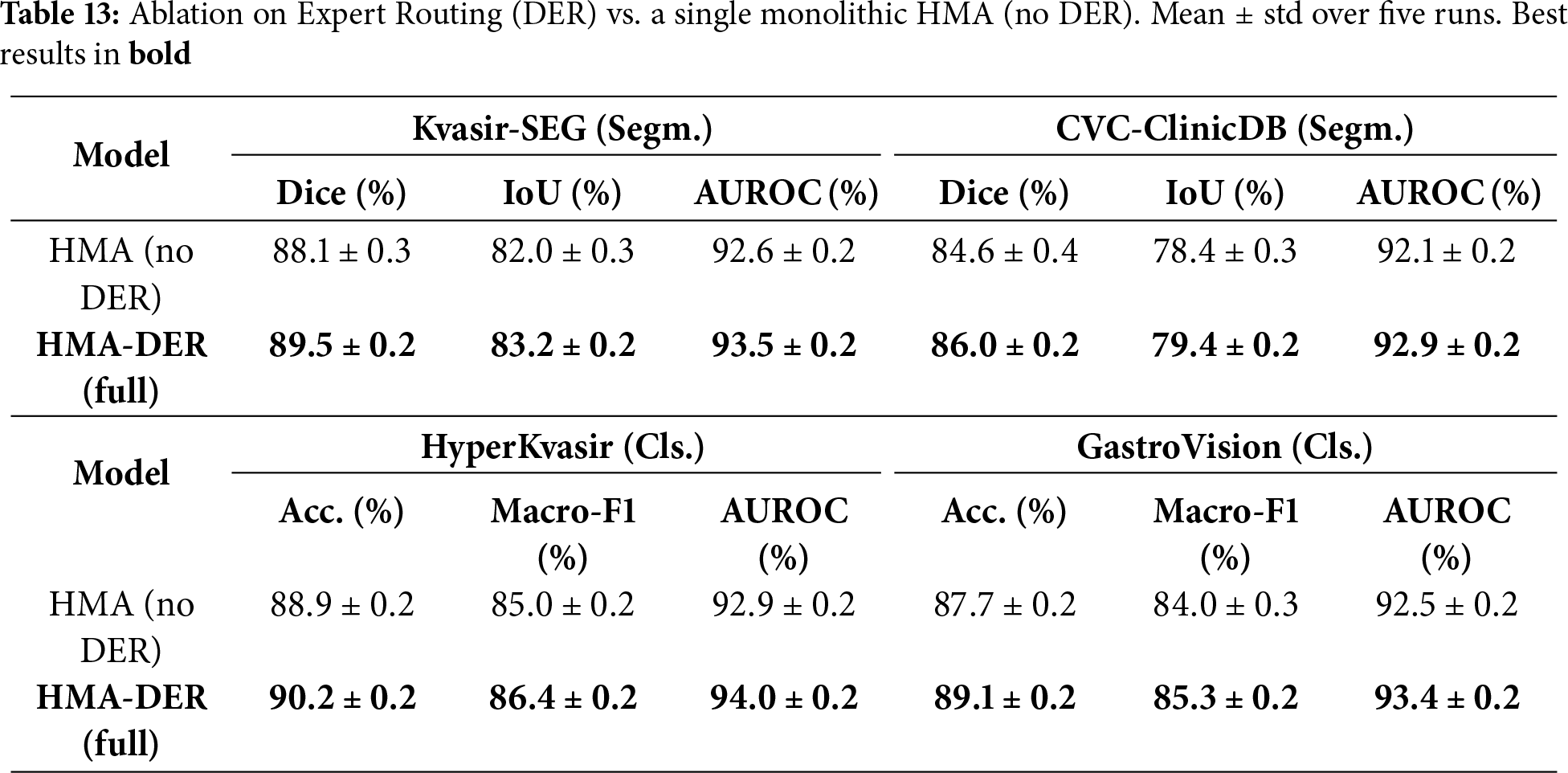
To isolate the contribution of the Dynamic Expert Routing, we compare the full HMA-DER against a single monolithic HMA variant in which the routing network and expert heads are removed and replaced by a single classifier head (all other components, losses, training schedules, data splits, and augmentations are kept identical). Table 13 reports mean
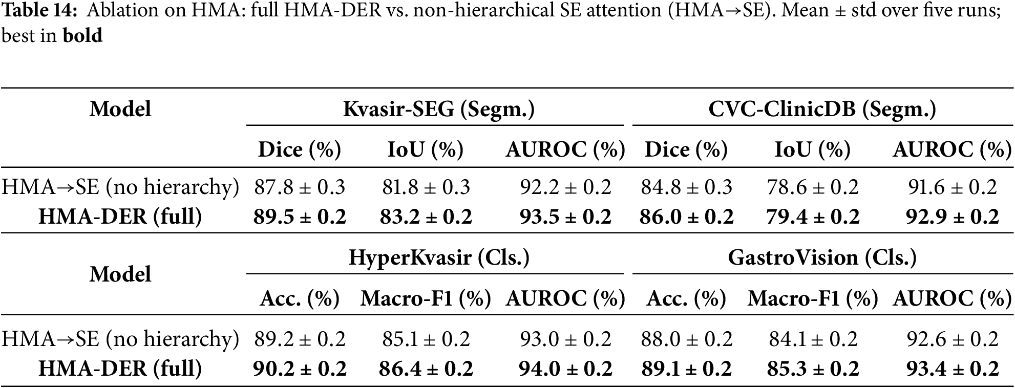
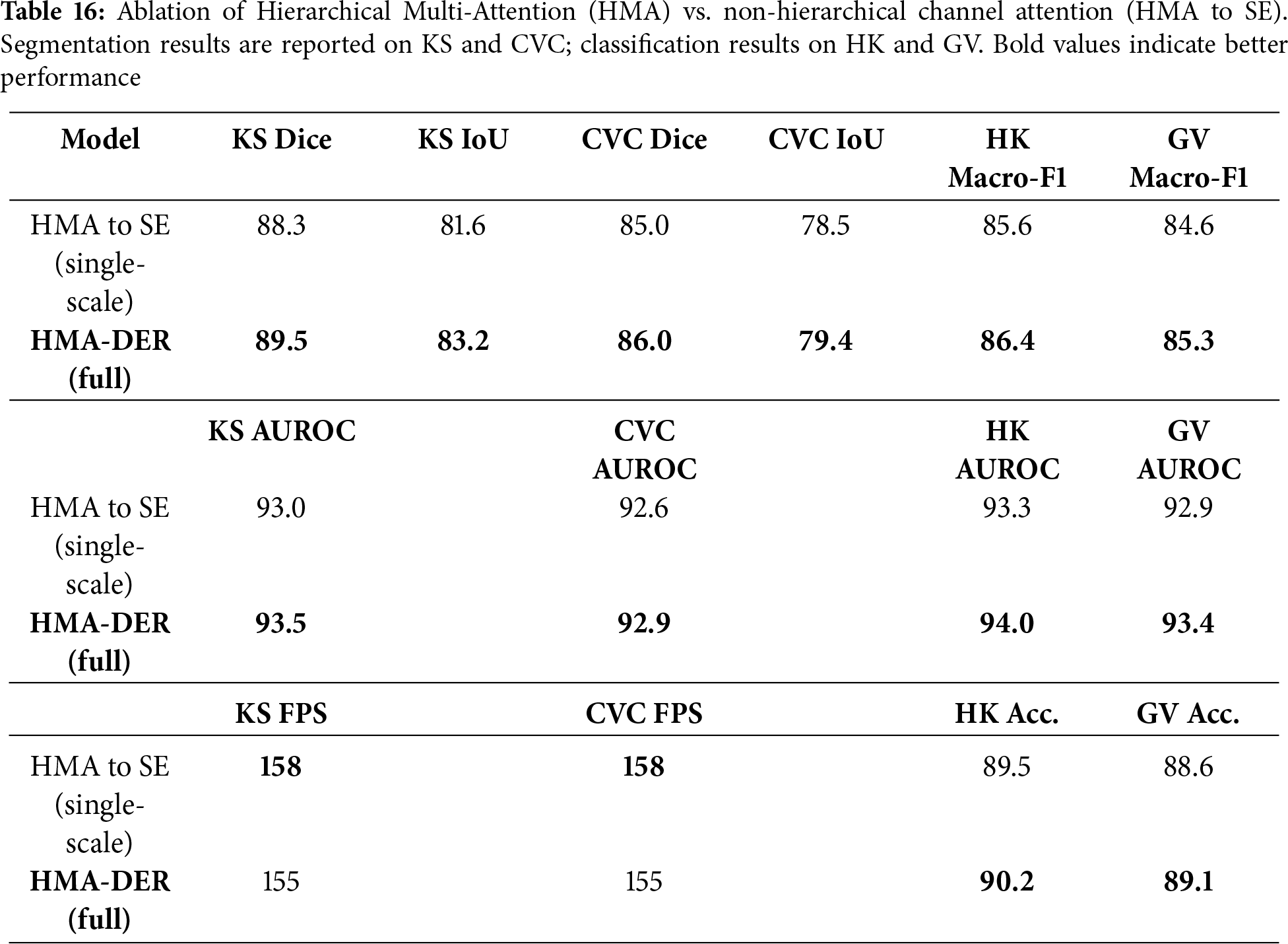
To quantify the contribution of HMA itself, we compare the full HMA-DER with a non-hierarchical variant where all hierarchical attention modules are replaced by standard Squeeze-and-Excitation (SE) blocks (channel-wise attention without global
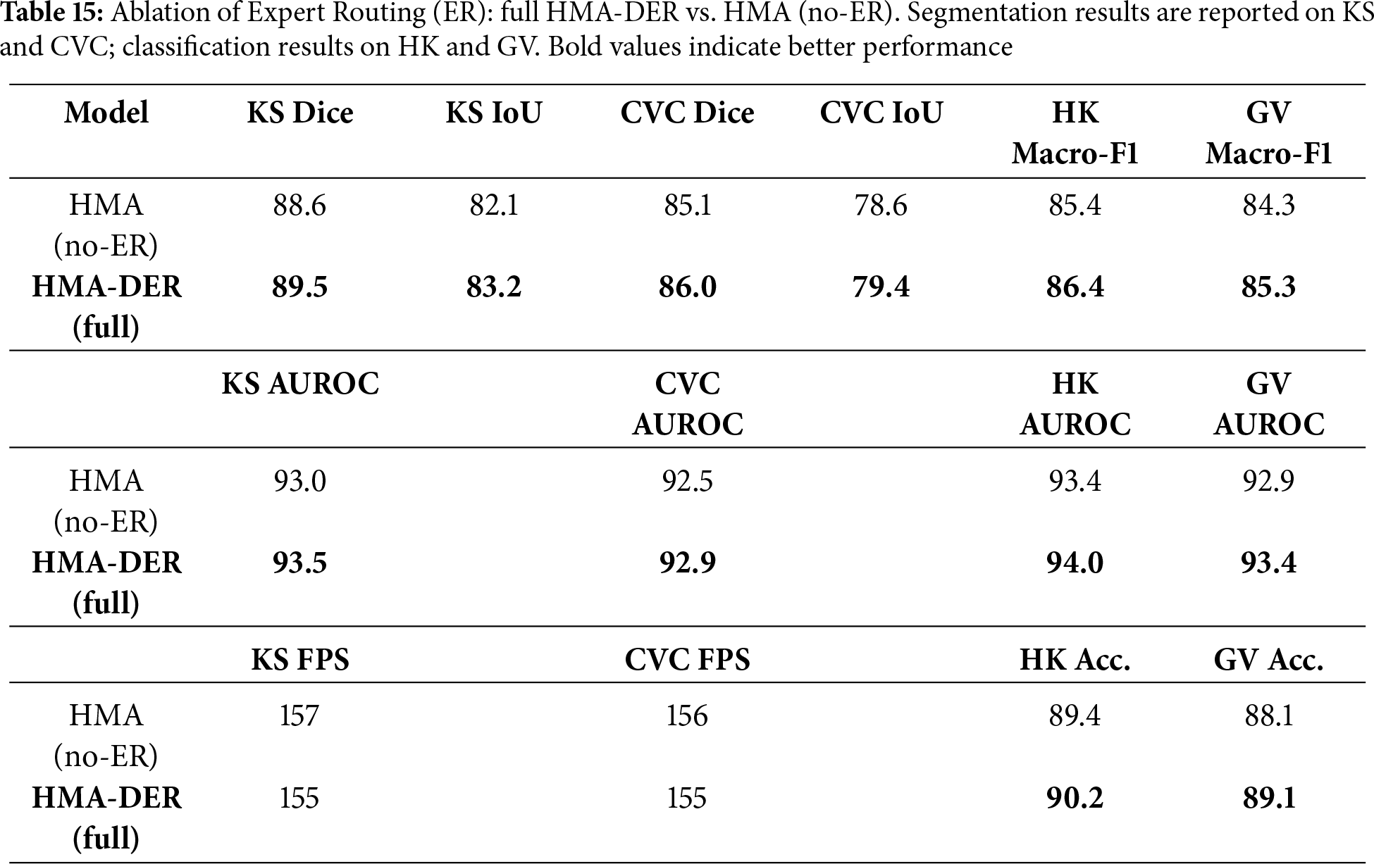
To quantify the standalone contribution of Expert Routing (Section 3.6), we compare the full HMA-DER to an HMA (no-ER) variant that disables routing and replaces the expert mixture with a single classifier head, keeping the backbone, losses, data splits, and training schedule identical to Table 3. As shown in Table 15, ER yields consistent gains across segmentation (Dice/IoU) and classification (Macro-F1/AUROC) with a small computational overhead, indicating that specializing hard/ambiguous cases improves decision quality without altering the underlying architecture.
To show the benefits of the hierarchical design, we replace HMA with a single-scale channel attention block (Squeeze-and-Excitation; SE) after the backbone. All other settings (losses, splits, scheduler; Table 3) stay the same. The HMA
Across all benchmarks, HMA-DER regularly beats classic CNNs, hybrid CNNs, transformers, ensembles, Siamese networks, and graph-based architectures. HMA-DER had the highest Dice and IoU scores on the Kvasir-SEG and CVC-ClinicDB segmentation datasets. This shows that the projected attention maps and the real polyp boundaries were better aligned. Residual connections are necessary for stable optimization in deep hierarchical networks since removing them makes performance worse on all datasets. The CAS-based explainability regularizer can improve both interpretability and accuracy, which will improve predictive performance and clinical alignment. Lastly, robustness-oriented augmentations greatly improve generalization when acquisition changes and make the model less sensitive to domain shifts.
Evaluating CAD systems requires a clinical understanding of false negatives (FNs) and false positives. In the HyperKvasir dataset’s ulcer and erosion categories, small, low-contrast, or partially occluded lesions without clear visual borders are often false negatives. Even skilled endoscopists sometimes have trouble with cases that are visually subtle. But most false positives come from mucosal folds, specular reflections, and minor lighting flaws that make materials look like lesions.
The confusion matrices (Fig. 15) show that the average false-negative rate for all datasets is 6.3% and the average false-positive rate is 4.9%. False negatives can delay diagnosis and the progression of illness, rendering them more clinically significant. False positives frequently need follow-up endoscopies that aren’t urgent. These add to the workload of diagnosing, but don’t provide any clinical risk. HMA-DER’s hierarchical attention and expert routing modules focus on visual signals that are important for diagnosis and send cases with low confidence to experts for refining. This cuts down on mistakes. This combination makes the model safer to use in clinical settings by lowering false negatives by 2–3.
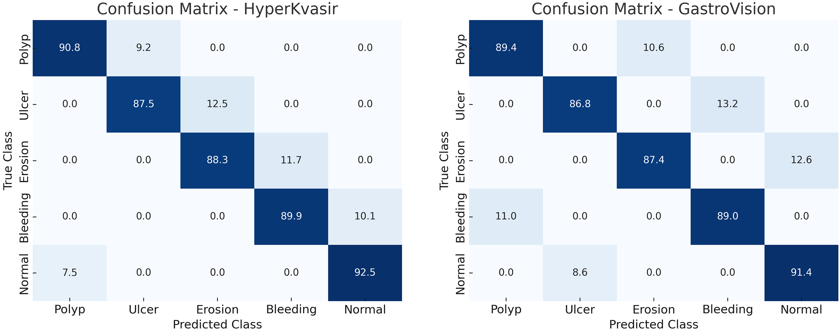
Figure 15: Confusion matrices illustrating the classification performance of the proposed HMA-DER model on the HyperKvasir and GastroVision datasets
The cross-dataset validation study shows how useful it is in the actual world. HMA-DER is competitive on diverse datasets even when the domain and category change. This shows that it learns representations that can be used in other contexts. The performance loss compared to in-domain evaluation, on the other hand, shows that medical imaging has an issue with distributional shift. Training on several datasets dramatically narrows the generalization gap. This indicates that federated or multi-institutional training would enhance HMA-DER robustness in subsequent deployments. In addition to quantitative improvements, model explainability is essential. HMA-DER uses CAS regularization to match attention maps with expert annotations, which makes its outputs credible and easy for doctors to understand. This alignment helps endoscopists trust AI-assisted solutions and may help them become more common in the clinic. The strong connection between explainability and prediction performance makes the accuracy-interpretability trade-off harder to understand.
HMA-DER is a hierarchical multi-attention framework for analyzing images of the gastrointestinal tract. It uses dilation-based receptive field expansion, residual connections, and explainability-aware CAS regularization. Full tests on Kvasir-SEG, CVC-ClinicDB, HyperKvasir, and GastroVision indicate that HMA-DER does better than strong CNN, hybrid, transformer, ensemble, Siamese, and graph-based baselines in both segmentation and classification. HMA-DER improves Dice by 2.4% and AUROC by 1.1% on Kvasir-SEG compared to the best baseline (MedT). It gets 1.7% more Dice and 1.2% more AUROC on CVC-ClinicDB. HMA-DER beats MedT in macro-F1 by 1.4% on HyperKvasir and 1.6% on GastroVision in big diagnostic datasets. It also has the highest AUROC values in all settings. These advancements establish a new benchmark for dependable and elucidated gastrointestinal diagnostics. The ablation study showed that each design feature made a difference. Without hierarchical multi-attention, performance declined by as much as 3.0%, although this was the best way to improve performance. Dilation-based receptive field expansion made datasets better by 1.5%–2%, but residual connections kept optimization going, stopping 2%–3% drops. The CAS-based regularizer made HyperKvasir easier to understand and more accurate, raising the macro-F1 score by almost 3.0%. Augmentations that focused on robustness enhanced cross-center generalization, while training on many datasets closed the domain gap by more than 3.0% compared to training on a single dataset.
Even though the results look good, there are a lot of limitations that need to be acknowledged. The approach employs four public datasets for supplementary segmentation and classification tasks, which may not comprehensively represent real-world endoscopic diversity. Difficult to attain resilience against infrequent image artifacts and severe acquisition conditions. The CAS-based regularizer is good at matching explanations with expert maps, although it hasn’t been tested in clinical user trials yet. There will be many ways to deal with these limits in the future. Validating bigger multi-center cohorts and video-based endoscopic datasets makes clinical scaling possible. Federated and ongoing learning can make distributional shift robustness better and let institutions use it without having to share data. Incorporating uncertainty estimation and active learning strategies will improve reliability under rare or unseen conditions. Finally, human-in-the-loop evaluations will be critical to assess the usability of CAS-driven explanations in real diagnostic workflows.
Acknowledgement: Not applicable.
Funding Statement: Princess Nourah bint Abdulrahman University Researchers Supporting Project number (PNURSP2025R77), Princess Nourah bint Abdulrahman University, Riyadh, Saudi Arabia.
Author Contributions: The authors confirm contribution to the paper as follows: study conception and design: Sara Tehsin, Inzamam Mashood Nasir, Wiem Abdelbaki; data collection: Fadwa Alrowais, Khalid A. Alattas, Sultan Almutairi; analysis and interpretation of results: Sara Tehsin, Inzamam Mashood Nasir, Radwa Marzouk; draft manuscript preparation: Wiem Abdelbaki, Fadwa Alrowais, Radwa Marzouk. All authors reviewed the results and approved the final version of the manuscript.
Availability of Data and Materials: The implementation of this work is available at https://github.com/imashoodnasir/Accurate-Gastrointestinal-Disease-Diagnosis (accessed on 16 November 2025).
Ethics Approval: Not applicable.
Conflicts of Interest: The authors declare no conflicts of interest to report regarding the present study.
References
1. Jha D, Smedsrud PH, Riegler MA, Halvorsen P, De Lange T, Johansen D, et al. Kvasir-seg: a segmented polyp dataset. In: International conference on multimedia modeling. Cham, Switzerland: Springer; 2019. p. 451–62. [Google Scholar]
2. Sushama G, Menon GC. Flexible colon polyp detection: a dual mode approach for detection and segmentation of colon polyps with optional inpainting for specular highlight mitigation. SN Comput Sci. 2024;5(5):641. [Google Scholar]
3. Jiang Y, Hu Y, Zhang Z, Wei J, Feng CM, Tang X, et al. Towards a benchmark for colorectal cancer segmentation in endorectal ultrasound videos: dataset and model development. In: International Conference on Medical Image Computing and Computer-Assisted Intervention; 2024 Oct 6–10; Marrakesh, Morocco. Cham, Switzerland: Springer; 2024. p. 732–42. [Google Scholar]
4. Borgli H, Thambawita V, Smedsrud PH, Hicks S, Jha D, Eskeland SL, et al. HyperKvasir, a comprehensive multi-class image and video dataset for gastrointestinal endoscopy. Sci Data. 2020;7(1):283. doi:10.1038/s41597-020-00622-y. [Google Scholar] [PubMed] [CrossRef]
5. Ali S, Jha D, Ghatwary N, Realdon S, Cannizzaro R, Salem OE, et al. A multi-centre polyp detection and segmentation dataset for generalisability assessment. Sci Data. 2023;10(1):75. doi:10.1038/s41597-023-01981-y. [Google Scholar] [PubMed] [CrossRef]
6. He K, Zhang X, Ren S, Sun J. Deep residual learning for image recognition. In: Proceedings of the IEEE Conference on Computer Vision and Pattern Recognition; 2016 Jun 27–30; Las Vegas, NV, USA. p. 770–8. [Google Scholar]
7. Huang G, Liu Z, Van Der Maaten L, Weinberger KQ. Densely connected convolutional networks. In: Proceedings of the IEEE Conference on Computer Vision and Pattern Recognition; 2017 Jul 21–26; Honolulu, HI, USA. p. 4700–8. [Google Scholar]
8. Chen J, Lu Y, Yu Q, Luo X, Adeli E, Wang Y, et al. Transunet: transformers make strong encoders for medical image segmentation. arXiv:2102.04306. 2021. [Google Scholar]
9. Valanarasu JMJ, Oza P, Hacihaliloglu I, Patel VM. Medical transformer: gated axial-attention for medical image segmentation. In: International Conference on Medical Image Computing and Computer-Assisted Intervention; 2021 Sep 27–Oct 1; Strasbourg, France. Cham, Switzerland: Springer; 2021. p. 36–46. [Google Scholar]
10. Huang SY, Hsu WL, Hsu RJ, Liu DW. Fully convolutional network for the semantic segmentation of medical images: a survey. Diagnostics. 2022;12(11):2765. doi:10.3390/diagnostics12112765. [Google Scholar] [PubMed] [CrossRef]
11. Weng W, Zhu X. INet: convolutional networks for biomedical image segmentation. IEEE Access. 2021;9:16591–603. doi:10.1109/access.2021.3053408. [Google Scholar] [CrossRef]
12. Chen LC, Zhu Y, Papandreou G, Schroff F, Adam H. Encoder-decoder with atrous separable convolution for semantic image segmentation. In: Proceedings of the European Conference on Computer Vision (ECCV); 2018 Sep 8–14; Munich, Germany. p. 801–18. [Google Scholar]
13. Isensee F, Jaeger PF, Kohl SA, Petersen J, Maier-Hein KH. nnU-Net: a self-configuring method for deep learning-based biomedical image segmentation. Nat Methods. 2021;18(2):203–11. doi:10.1038/s41592-020-01008-z. [Google Scholar] [PubMed] [CrossRef]
14. Fan DP, Ji GP, Zhou T, Chen G, Fu H, Shen J, et al. Pranet: parallel reverse attention network for polyp segmentation. In: Proceedings of the International Conference on Medical Image Computing and Computer-Assisted Intervention; 2020 Oct 4–8; Lima, Peru. p. 263–73. [Google Scholar]
15. Dosovitskiy A, Beyer L, Kolesnikov A, Weissenborn D, Zhai X, Unterthiner T, et al. An image is worth 16 × 16 words: transformers for image recognition at scale. arXiv:2010.11929. 2020. [Google Scholar]
16. Liu Z, Lin Y, Cao Y, Hu H, Wei Y, Zhang Z, et al. Swin transformer: hierarchical vision transformer using shifted windows. In: Proceedings of 2021 IEEE/CVF International Conference on Computer Vision (ICCV); 2021 Oct 10–17; Montreal, QC, Canada. p. 10012–22. [Google Scholar]
17. Cao H, Wang Y, Chen J, Jiang D, Zhang X, Tian Q, et al. Swin-unet: unet-like pure transformer for medical image segmentation. In: European conference on computer vision. Cham, Switzerland: Springer; 2022. p. 205–18. [Google Scholar]
18. Selvaraju RR, Cogswell M, Das A, Vedantam R, Parikh D, Batra D. Grad-cam: visual explanations from deep networks via gradient-based localization. In: Proceedings of 2017 IEEE International Conference on Computer Vision (ICCV); 2017 Oct 22–29; Venice, Italy. p. 618–26. [Google Scholar]
19. Yona G, Greenfeld D. Revisiting sanity checks for saliency maps. arXiv:2110.14297. 2021. [Google Scholar]
20. Ivanovs M, Kadikis R, Ozols K. Perturbation-based methods for explaining deep neural networks: a survey. Pattern Recognit Lett. 2021;150:228–34. doi:10.1016/j.patrec.2021.06.030. [Google Scholar] [CrossRef]
21. Petsiuk V, Das A, Saenko K. Rise: randomized input sampling for explanation of black-box models. arXiv:1806.07421. 2018. [Google Scholar]
22. Imambi S, Prakash KB, Kanagachidambaresan G. PyTorch. In: Programming with TensorFlow: solution for edge computing applications. Cham, Switzerland: Springer; 2021. p. 87–104. [Google Scholar]
23. Simonyan K, Zisserman A. Very deep convolutional networks for large-scale image recognition. arXiv:1409.1556. 2014. [Google Scholar]
24. Szegedy C, Ioffe S, Vanhoucke V, Alemi A. Inception-v4, inception-resnet and the impact of residual connections on learning. Proc AAAI Conf Artif Intell. 2017;31:1–15. doi:10.1609/aaai.v31i1.11231. [Google Scholar] [CrossRef]
25. Hu J, Shen L, Sun G. Squeeze-and-excitation networks. In: Proceedings of the 2018 IEEE/CVF Conference on Computer Vision and Pattern Recognition; 2018 Jun 18–23; Salt Lake City, UT, USA. p. 7132–41. [Google Scholar]
26. Valdenegro-Toro M. Sub-ensembles for fast uncertainty estimation in neural networks. In: Proceedings of the 2023 IEEE/CVF International Conference on Computer Vision Workshops (ICCVW); 2023 Oct 2–6; Paris, France. p. 4119–27. [Google Scholar]
27. Duque Domingo J, Medina Aparicio R, Gonzalez Rodrigo LM. Improvement of one-shot-learning by integrating a convolutional neural network and an image descriptor into a siamese neural network. Appl Sci. 2021;11(17):7839. doi:10.3390/app11177839. [Google Scholar] [CrossRef]
28. Vrahatis AG, Lazaros K, Kotsiantis S. Graph attention networks: a comprehensive review of methods and applications. Future Internet. 2024;16(9):318. doi:10.3390/fi16090318. [Google Scholar] [CrossRef]
29. Zhang Y, Liu H, Hu Q. Transfuse: fusing transformers and cnns for medical image segmentation. In: International Conference on Medical Image Computing and Computer-Assisted Intervention; 2021 Sep 27–Oct 1; Strasbourg, France. Cham, Switzerland: Springer; 2021. p. 14–24. [Google Scholar]
30. Dong B, Wang W, Fan DP, Li J, Fu H, Shao L. Polyp-pvt: polyp segmentation with pyramid vision transformers. arXiv:2108.06932.2021. [Google Scholar]
31. Abian AI, Raiaan MAK, Jonkman M, Islam SMS, Azam S. Atrous spatial pyramid pooling with swin transformer model for classification of gastrointestinal tract diseases from videos with enhanced explainability. Eng Appl Artif Intell. 2025;150:110656. doi:10.1016/j.engappai.2025.110656. [Google Scholar] [CrossRef]
32. Heidari M, Kazerouni A, Soltany M, Azad R, Aghdam EK, Cohen-Adad J, et al. Hiformer: hierarchical multi-scale representations using transformers for medical image segmentation. 47. In: Proceedings of the 2023 IEEE/CVF Winter Conference on Applications of Computer Vision (WACV); 2023 Jan 2–7; Waikoloa, HI, USA. p. 6202–12. [Google Scholar]
33. Jin X, Xie Y, Wei XS, Zhao BR, Chen ZM, Tan X. Delving deep into spatial pooling for squeeze-and-excitation networks. Pattern Recognit. 2022;121:108159. doi:10.1016/j.patcog.2021.108159. [Google Scholar] [CrossRef]
Cite This Article
 Copyright © 2026 The Author(s). Published by Tech Science Press.
This work is licensed under a Creative Commons Attribution 4.0 International License , which permits unrestricted use, distribution, and reproduction in any medium, provided the original work is properly cited.
 Downloads
 Citation Tools