
 Submit a Paper
 Propose a Special lssue
 Open Access
ARTICLE
Optimal Structure Determination for Composite Laminates Using Particle Swarm Optimization and Machine Learning
1 Automation Department, “Dunarea de Jos” University, Galati, 800008, Romania
2 Informatics Department, “Danubius” University, Galati, 800654, Romania
* Corresponding Author: Viorel Mînzu. Email:
(This article belongs to the Special Issue: Machine Learning in the Mechanics of Materials and Structures)
Computers, Materials & Continua 2026, 87(1), 22 https://doi.org/10.32604/cmc.2026.075619
Received 05 November 2025; Accepted 06 January 2026; Issue published 10 February 2026
 View Full Text
 Download PDF
Abstract
This work addresses optimality aspects related to composite laminates having layers with different orientations. Regression Neural Networks can model the mechanical behavior of these laminates, specifically the stress-strain relationship. If this model has strong generalization ability, it can be coupled with a metaheuristic algorithm–the PSO algorithm used in this article–to address an optimization problem (OP) related to the orientations of composite laminates. To solve OPs, this paper proposes an optimization framework (OFW) that connects the two components, the optimal solution search mechanism and the RNN model. The OFW has two modules: the search mechanism (Adaptive Hybrid Topology PSO) and the Prediction and Computation Module (PCM). The PCM undertakes all the activities concerning the OP at hand: the stress-strain model, constraints checking, and computation of the objective function. Two case studies about the layers’ orientations of laminated specimens are conducted to validate the proposed framework. The specimens belong to “Off-axis oriented specimens” and are subjects of two OPs. The algorithms for AHTPSO and for the two PCMs (one for each problem) are proposed and implemented by MATLAB scripts and functions. Simulations are carried out for different initial conditions. The solutions demonstrated that the OFW is effective and has a highly acceptable computational complexity. The limitation of using the OFW is the generalization ability of the RNN model or any other regression models. To harness the RNN model efficiently, it must have a very good generalization power. If this condition is met, the OFW can be integrated into any design process to make optimal choices of the layers’ orientations.Keywords
The mechanical behavior of composite laminates with various layer orientations [1] is studied based on data collected through tensile tests, numerical integration, simulations, and Machine Learning (ML) models. These models have a very important characteristic: their ability to generalize; they predict parameter values for new composite laminates that did not contribute to the training data. Regression models, built using machine learning models, predict parameter values used in complex analysis of mechanical load behavior. There is no need to conduct expensive tensile tests or time-consuming simulations.
In a previous work [2], data on the mechanical load behavior of a specific group of composite laminates with different layer orientations were collected. These data were used with ML algorithms to develop regression models that accurately predict stress based on specific parameters. After analyzing these regression models, the model based on the Regression Neural Network (RNN) has demonstrated a strong ability to generalize to new layer orientations of the Composite Laminates (CLs). The question that arises from having such a prediction tool is whether it can be used to find the combination of orientations (angles) that optimizes an objective function. The latter, along with the optimization method, could be integrated into a design process for CLs. Our paper provides a constructive answer to this question.
This paper proposes an optimization framework (OFW) for solving optimization problems related to CLs. To test the OFW, two optimization problems are formulated and solved through simulation studies. The framework has a few characteristics:
• A specific version of the PSO algorithm enables the search mechanism that leads to optimal solutions.
• The RNN, developed in our previous work, models the mechanical load behavior of CLs.
• The OFW has two modules that communicate with each other: one implements the PSO algorithm, and the other, called the Prediction and Computation Module (PCM), undertakes all components related to the optimization problem at hand.
The PCM handles all aspects related to the OP, including prediction with the RNN, constraints checking, and calculating the objective function. This way, the OFW is systematically organized. If a new optimization problem must be solved, only the PCM needs updating; the module implementing PSO only has to update the instructions that call the PCM and adjust its parameters’ values based on the OP to solve.
The main objective of this presentation is to propose the OFW and its constitutive algorithms. The emphasis is placed on implementing the PCM because the PSO algorithm is widely known, and this paper briefly recalls the effective version used—the Adaptive Hybrid Topology PSO.
To describe the OFW and implement the PCM, the authors proposed two optimization problems dedicated to CLs with various layer orientations. The specimens selected for optimization belong to a specific group called “Off-axis oriented specimens”. To keep them simple, the two OPs have formulations with straightforward constraints and objective functions, but the computational complexity required to find the optimal solution is not trivial. To ensure strong generalization ability, the RNN previously developed by the authors is utilized. The RNN model is already stored in a “workspace” file, from which it is loaded into programs implementing the OFW.
Using artificial intelligence in composite material science, including ML and deep learning, has also significantly expanded the use of regression algorithms. Our article follows the general trend of using these models along with optimization techniques.
From the perspective of materials science specialists, the literature on composite materials includes two main categories of articles using AI techniques: one focused on determining material properties (e.g., Young’s modulus) and the other on understanding relationships between different parameters, such as mechanical behavior (for example, stress-strain curves).
Ref. [3] demonstrates how neural networks can enhance the accuracy of predicting dynamic mechanical properties. Ref. [4] reviews different ML and deep learning methods for predicting composite material (CM) properties such as strength, stiffness, elasticity, plasticity, ductility, brittleness, toughness, and hardness. ML algorithms can also predict the Young’s modulus of polymer composites reinforced with carbon nanotubes [5], enabling the development of new materials.
Ref. [6] utilizes different ML models, including Random Forest, Gradient Boosting, and XGBoost, to evaluate how multi-stacking learning techniques perform relative to traditional approaches. Other methods [7] yield predictions by examining an image of the material’s microstructure and utilizing knowledge of the constitutive models for fibers and matrix, without engaging in physically-based calculations.
The Convolutional Neural Network–Long and Short-Term Memory [8] model forecasts the mechanical properties of carbon fiber composites, achieving predictions within 5% of the actual tensile experimental results. Predictions are made with various ML models [9], including Ridge Regression, Bayesian Ridge Regression, Lasso Regression, CatBoost, K-Nearest Neighbors, Decision Tree, Random Forest, and Support Vector Regression. The K-Nearest Neighbors and CatBoost models offered the most accurate predictions for E and σ.
Convolutional neural networks, along with principal component analysis, can effectively predict stress-strain responses based on microstructural images of composites [10].
The programs included in the proposed OFW are written in MATLAB R2015b. In this field, the algorithms are strongly dependent on the language and libraries used to develop them. For technical details on regression models and RNNs, the reader can consult references [11–15]. This should help better understand the proposed algorithms.
The literature provides a vast array of references on PSO. The references mentioned hereafter can help newcomers in the field learn the basic concepts of this metaheuristic and understand the AHTPSO algorithm; the latter implements the search mechanism of the optimal solution. The basics of PSO can be found in [16–18]. Besides other references, the concepts of hybrid topology and adaptive PSO are explained in [17–20]. Numerous papers describe the use of different PSO versions across various fields. Ref. [21], for example, highlights numerous applications of metaheuristic algorithms, including PSO, in process engineering. Applications of metaheuristics combined with ML predictions–like in this article–are discussed in [22,23].
The authors consider that this work has the following contributions:
• The structure of the optimization framework and the method employed to solve optimization problems involving composite laminates.
• A specific implementation of the OFW through collaboration between the searching mechanism (AHTPSO) and PCM. The PCM handles all parts of the addressed OP: the RNN model for mechanical load behavior, constraint checking, and the calculation of the objective function.
• The presentation and analysis of two case studies that demonstrate the effectiveness of our approach in addressing optimality aspects in designing the CLs.
2 An Accurate Regression Model of Stress-Strain Dependence
In their previous research project, the authors created an accurate regression model of stress-strain dependence for composite laminates with layers of different orientations. This model is an RNN that has excellent generalization capabilities [2] and was taken over in this study for the PCM’s implementation. To develop regression models using ML algorithms, data on the mechanical load behavior of composite laminates with different layer orientations were collected through tensile tests and simulations.
The CL specimens are made of AS4 carbon fiber and 8552 epoxy resin matrix. A group of twelve specimens was analyzed using precise finite element simulations. Each specimen is characterized by its combination of layer orientations (angles), α1, α2, …, α16. Two specimens with their layer orientations are provided in Fig. A1 of Appendix A.
For the simulation study, M data points were generated for each specimen. The M data points for specimen Sk, where k = 1, ..., 12, only cover the linear (elastic) zone of the stress-strain curves. They have the following structure:
Within the same research project, there are prediction models that also deal with the nonlinear (plastic) region. However, in most applications, the elastic area is used, and that is why it is the preferred option for optimization.
There are 12∙M data points, which allowed us to construct regression models that predict the stress value of any specimen having the sixteen orientations and the load characterized by the given strain value. Our approach was based on supervised learning algorithms, considering the stress value as the label for each data point. In the present study, the authors used the more accurate ML model, which is an RNN. In the sequel, it will be referred to as RNN2, like in the article where we presented it [2].
Fig. 1 compares the true and predicted values of stress, “Response (Ss)”, for all the data points. RNN2 demonstrates very good accuracy and justifies its selection in the actual optimization study. Fig. A2 in Appendix A also shows the good accuracy in the testing phase of RNN2.
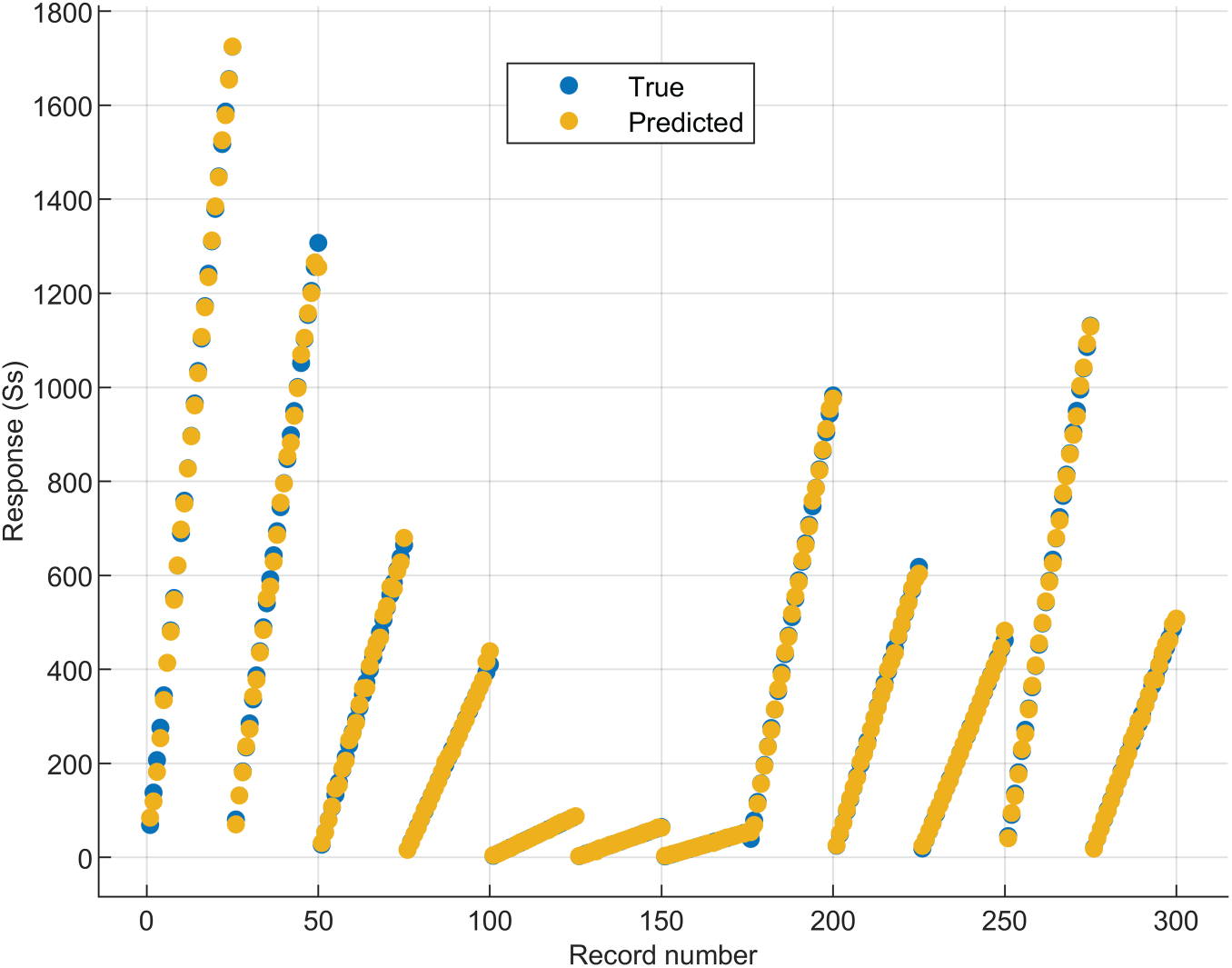
Figure 1: Training of RNN2: Predicted vs. real values for the twelve specimens
The generalization ability of the RNN2 model has been demonstrated for data points outside of the training and test datasets.
The question that arises from the existence of such a prediction tool is whether it can be used successfully to find the combination of orientations (angles) that optimizes an objective function. The latter can be incorporated into a design process for the composite laminates. Our work provides an answer to this question.
The main objective of our paper is to propose an optimization framework that combines a metaheuristic algorithm, specifically Particle Swarm Optimization, with an ML model of the CL, which is an RNN. The latter is a stress–strain regression model for the CL being considered. Fig. 2 below illustrates the proposed optimization framework.
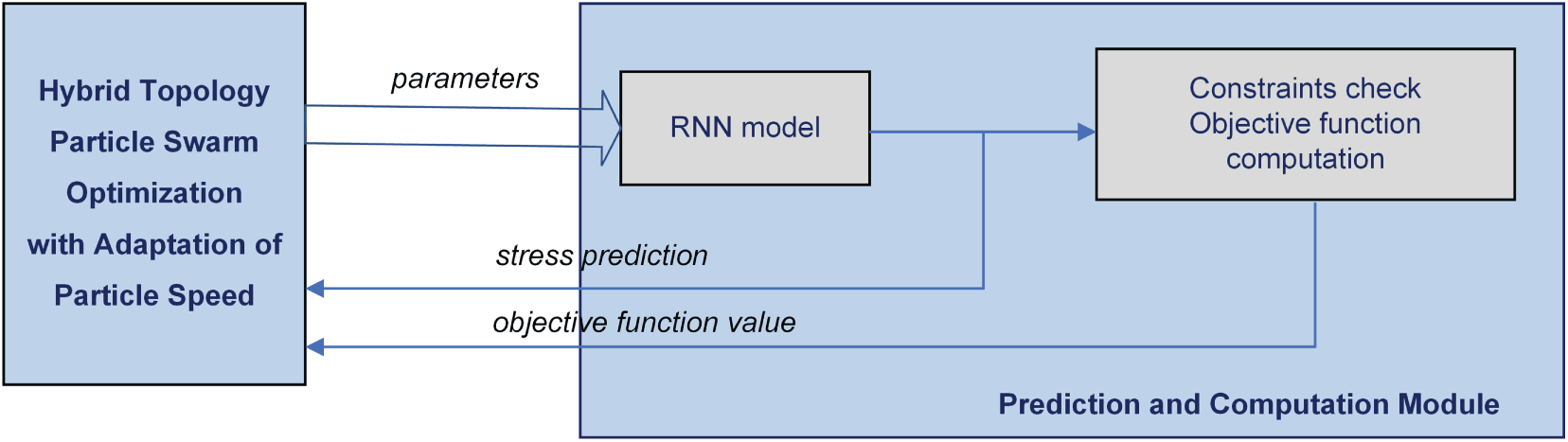
Figure 2: Structure of the optimization framework
Fig. 2 shows that the optimization framework is composed of two modules: the PSO algorithm and the Prediction and Computation Module (PCM). Informally, an OP is defined by three components:
• The model of the object or system subjected to optimization.
• The mathematical constraints that the optimal solutions must satisfy.
• The objective (cost) function is a mathematical expression that depends on decision variables and must be minimized or maximized.
The Prediction and Computation Module (PCM) handles all three components. The object model used for optimization is the model of the stress-strain relationship for the CL at hand. This is RNN2 in our case. As a programming unit, PCM is a function that receives the parameters defining a candidate solution, that is, a combination of orientation, and returns the predicted stress value and the cost function value J.
The AHTPSO module executes the full search process for the best solution. As is well-known, this is an iterative process that calls the PCM at each step to improve the swarm’s best solutions until it converges to the global optimal solution.
We must highlight that the novelty of this optimization framework lies in its systematic organization. The AHTPSO algorithm manages the search mechanism for the optimal solution and collaborates with the PCM, which reflects only the OP that must be solved. The authors do not aim to propose a PSO algorithm that is better than others. Different versions of PSO, like the AHTPSO algorithm, have proven effective in many applications for solving NP-hard problems. At convergence, the optimization framework finds the optimal solution, whose cost function value defines the performance index (J*) of the object or system.
To demonstrate its effectiveness, the proposed OFW will be used in the sequel to solve two case studies for Off-Axis Oriented Specimens. Solving the two OPs will help us in addressing specific implementation aspects of the two modules within the OFW.
An important aspect in the implementation of the proposed OFW is the communication between the AHTPSO and the PCM. The input arguments of the PCM, including the regression model, depend entirely on the OP’s nature. These arguments, which must be prepared, also make the AHTPSO algorithm dependent on the OPAs usual, its parameters need to be adjusted based on the solved OP.
We assume that readers interested in solving OPs using metaheuristics are familiar with the general PSO algorithm. To keep the paper self-contained, only elements that have improved the efficiency of PSO over time and were used in this study are recalled in the sequel. For example, references [16–18] can provide newcomers in the field with the basics of the PSO algorithms and how they can be used.
The algorithm used in this work is based on hybrid topology particle swarm optimization (HTPSO) [18–20], which is an improved version of the general PSO metaheuristic with better communication abilities among particles. The global topology corresponds to a network where particles communicate through the global best solution (Pgbest) encountered at a certain step of the swarm’s evolution. HTPSO also uses a local topology of the swarm, regarded as a communication network. The local topology involves the existence, for any particle #i, of a “social neighborhood”, i.e., a set of 3–5 particles that inform particle #i about their best personal experience. These neighborhoods are defined in a deterministic or random manner at each step of the algorithm (see [23]). The particle #i will determine the local best solution,
A new term appears in the speed equation containing C3 and rand3 (see [18]). Hence, the update of the speed and position at the next step, t + 1, is performed using the following equations:
4.1.2 Adaptation of Particle Speed-AHTPSO
The HTPSO can be enhanced with an efficient technique, the adaptation of particle speed, which will produce the Adaptive HTPSO. This technique modifies the coefficients C1, C2, C3, and w during the searching process (see [18,19]). The objective is to adapt them to the phase of the search process and prepare the algorithm’s convergence. The adaptation is achieved by a linear increase in the coefficients C1, C2, and C3 between their minimum and maximum values. At the same time, the parameter w decreases as shown below:
T is the estimated or maximum number of steps until convergence.
This work uses an AHTPSO algorithm, which improves the convergence.
There are also other new improvements, but it is not the purpose of this research to provide a very competitive version of the PSO algorithm. The validation of the optimization framework for CLs is our main goal. Anyhow, the runnings of AHTPSO proved that the efficiency of the proposed algorithm is very satisfactory.
4.2 Prediction and Computation Module
The PCM is implemented by a function that handles the three components of an OP mentioned above. This function incorporates all the elements that define the problem and all the computing details. As a result, the AHTPSO module manages the search process, while the PCM incorporates the OP’s features. This fact gives the proposed optimization framework a systematic character.
Because the OP refers to CL’s mechanical behavior, two input arguments are mandatory. One is the RNN, that is, the model of the stress-strain relationship for the CL. Another argument is the strain value that characterizes the CL’s load. In this way, PCM has all that is necessary to predict the stress value, which is further used to calculate the cost function. The other input arguments vary based on the OP’s nature and are used for checking constraints and computing the cost function (J).
4.3.1 The Context of the Off-Axis Oriented Specimens
This subsection explains the reasons that led us to formulate the OPs as shown in the following sections. The arguments should be viewed in the context of composite materials science [2].
To understand the first OP statement, first, we present the context of the mechanical behavior of a certain group of composite laminates. It is about the group of “Off-axis oriented specimens”: S2 ([±20]8), S3 ([±30]8), S4 ([±45]8), S5 ([±60]8), and S6 ([±70]8). The fibers are oriented at angles diverging from the principal stress direction. This is a special case where there are two angles (a and −a), and the sequence is repeated eight times. But the pattern can be generalized using eight positive values as follows:
The stress-strain curves for three off-axis oriented laminates, S2, S3, and S4, are shown in Fig. 3. They exhibit different mechanical behaviors as fiber orientations gradually diverge from the load axis. These CLs show a decrease in stiffness and tensile strength as the fiber alignment shifts further off the load axis. Within the elastic region, the stress-strain curve remains linear, but the stiffness drops evidently with larger fiber angles.
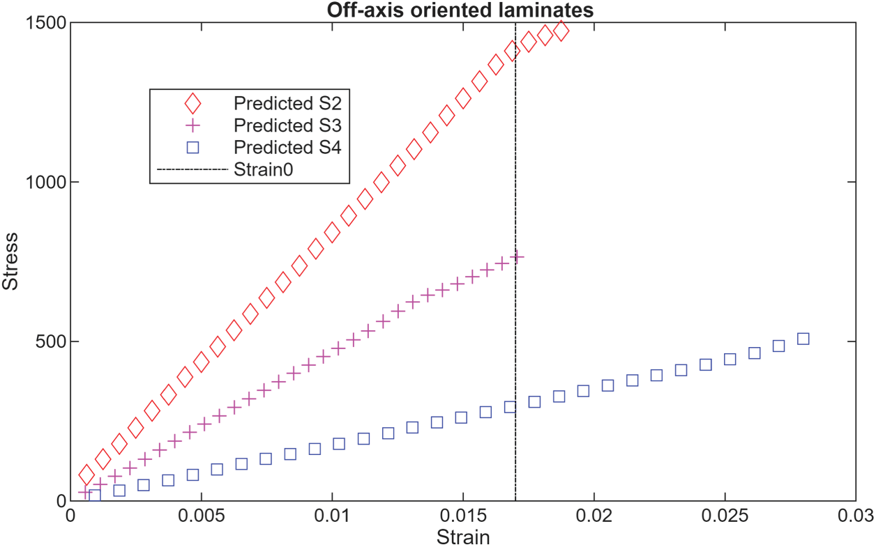
Figure 3: Stress-strain curves for three off-axis oriented laminates
This reduction can be explained because the fibers are not fully aligned with the tensile load, which causes the matrix to bear more load. As the fiber angle increases, the stiffness continues to decrease. The fibers are now mainly aligned to resist shear loads rather than axial loads.
Comparing the stress values across these curves requires a reference interval for strain variation. Since the maximum strain values defining the elastic zone for S2, S3, and S4 are 0.0187, 0.0170, and 0.0279, respectively, we used the common interval [0, Strain0], where Strain0 is the maximum value for S3 (0.017).
In Case Study 1, we state an optimization problem (OP1) that will find the orientations of CL, like in Eq. (2), under certain conditions. The optimal solution must make a trade-off between the specimen’s stiffness and good behavior to shear loads. We consider that the optimal solution must meet two conditions:
• The stress for the maximum strain, Strain0, must be a minimum of 1000 MPa.
• Its stress–strain curve must be the closest to the S3’s curve.
Remark 1: The first constraint sets a minimum stiffness requirement, so the optimal solution curve will tend to stay close to the S2 curve, which has a maximum value of 1500 MPa. The second constraint reflects the need for good resistance to shear loads, which means finding a solution as close as possible to the S3 curve.
The orientations of a CL meeting the pattern from Eq. (2) can be coded by the sequence of positive angles, [a1 a2 ... a8]. If we consider two specimens meeting Eq. (2), a natural way to express the distance between the two specimens’ orientations is the following value:
inspired by the Euclidean distance. In our case, S3 is the reference specimen whose pattern is encoded by [30/30/…30]. The stress-strain curve for the elastic and plastic zones can be considered as a function, y = stress(u), where u is the strain value and y is the resulting stress value.
After these preparations, OP1 can be stated as follows.
I. Model of the object (system) subjected to optimization
The object is defined by all specimens for which it holds:
•
• The RNN2 is a regression model of the stress-strain curve.
II. Constraints
III. Objective function
4.3.2 Description of the AHTPSO Algorithm
The reason the pseudocode of the AHTPSO algorithm is provided hereafter is not due to the novelty of this algorithm, even though it integrates the two improvements of PSO. However, its structure aligns with the PCM’s organization and the structure shown in Fig. 2. Algorithm 1 provides the pseudocode of the AHTPSO-CL algorithm.
Instruction #1 initializes N: the number of particles, n: the dimension of candidate solutions, T: the maximum number of steps until convergence, NF: the variables used to determine the convergence, the parameters used to limit the position (xmin and xmax) and the speed (vmax) of particles and to adapt the algorithm.
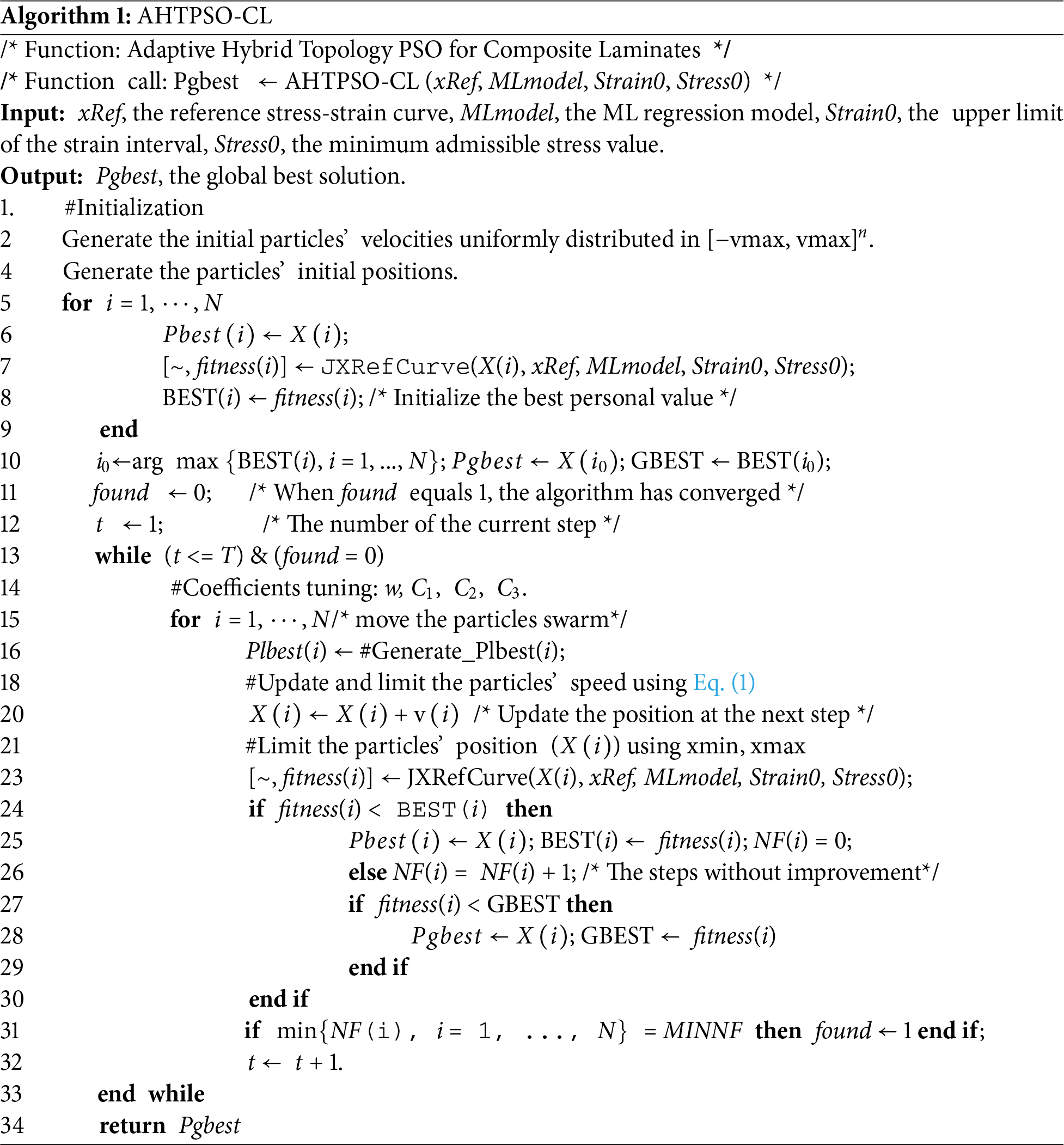
Instructions #7 and #23 call the cost function specific to the optimization problem OP1. This is named JXRefCurve, and it is described by Algorithm 2 in the next subsection. The arguments X(i), xRef, and MLmodel are, respectively, a candidate solution, the pattern of the reference curve, and the ML regression model of the composite laminate (an RNN in our case). Besides the cost value, J, the function JXRefCurve also returns the stress value for the point Strain0, which is useful in our study.
Instruction #10 determines the initial global best solution, Pgbest, and its cost value GBEST. The function #Generate_Plbest(i), which is not detailed here for simplicity, is called by instruction #16 and generates the local best solution using three informer particles (social neighbors).
4.3.3 The Objective Function for Case Study 1
Algorithm 2 is the pseudocode for the PCM corresponding to OP1. Its input and output arguments were presented in the previous section.
Its input argument x is a vector comprising only the positive angles of the pattern that defines a candidate solution. Instructions #1 through #5 are designed to assemble a data point for which a prediction will be made. According to instruction #6, the regression model, MLmodel, predicts the stress value for Strain0. The constraint that the stress value should be greater than or equal to Stress0 is checked by instructions #7 and #8. If this constraint is not met, then the cost J equals infinity. Otherwise, the value of J is computed by instructions #10–#13 using the Eq. (3).
Let us notice that all three components of OP1—model, constraints, and cost function—are addressed within this algorithm, which corresponds to PCM.
The entire optimization framework was implemented using MATLAB R2025b software, like the component running the RNN2 regression model. A typical execution of this program, which repetitively calls the objective function JXRefCurve, provides the following results:
Angles: 25.22/−25.22/27.53/−27.53/26.13/−26.13/26.94/−26.94/26.99/−26.99/26.86/−26.86/25.63/−25.63/28.08/−28.08/
The performance index J0 = 95.05.
The objective function is evaluated 6040 times during the search for the optimal solution. The call count to this function reflects the computational complexity of the solution-searching process.
Fig. 4 displays the stress-strain curve for the optimal solution and the off-axis specimens’ curves. The green curve lies between S2 and S3, with the maximum stress reaching exactly 1000 MPa.
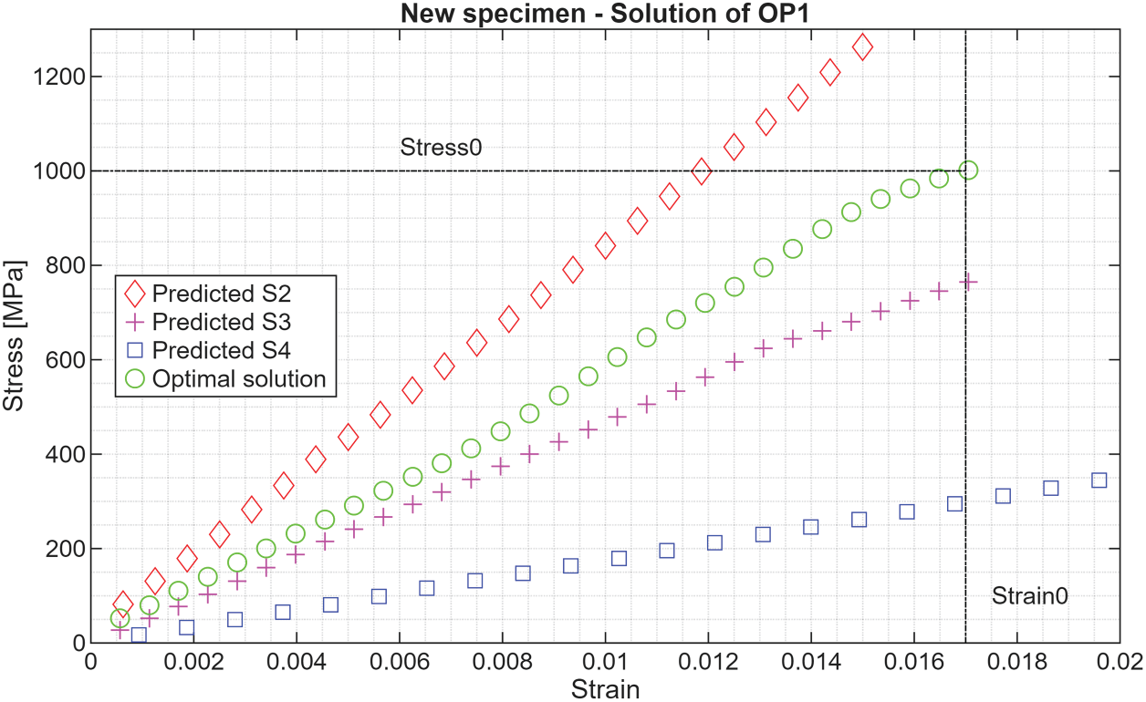
Figure 4: The optimal solution curve for OP1 compared to other oriented laminates
Let’s notice that the new specimen’s curve isn’t perfectly linear because the orientations are symmetric but different every two layers.
In this case, we consider the pattern [a/−a/a/−a/...a/−a], which characterizes the off-axis composite laminates S2–S6. For a specimen characterized by the angle a, the stress value for Strain0 can be regarded as a function S(a) = stress(a, Strain0), with Strain0 = 0.017.
We consider the second OP (OP2), which searches for the specimen with the pattern as before and whose maximum stress value, S(a), is closest to an imposed value S0. OP2 can be stated as follows.
I. Model of the object subjected to optimization
The object is defined by all specimens for which it holds:
•
• The RNN2 is a regression model of the stress-strain curve.
II. Constraints
There are no constraints except for the research domain,
III. Objective function
The solution will specify the value of a that yields the performance index J0.
Within the optimization framework, we retain the same AHTPSO algorithm, but we need to redefine the PCM, which is the function called by the intelligent searching mechanism. Algorithm 3 is the pseudocode description of the PCM for this problem.
Instructions #7 and #23 of Algorithm 1 must be slightly modified to call the function JfixPoint. The argument xRef has disappeared, and x is now just a scalar. The other parameters of the AHTPSO remained unchanged because they are suitable for OP2 as well.
The complete optimization framework was developed with MATLAB R2025b, similar to the component that executes the RNN2 regression model. A typical run of this program, which repeatedly invokes the objective function JFixPoint, yields the following results:
Optimal a = 26.43; J0 = 1.136868e−13; S0 = 1000.00 MPa.
The optimal orientation: 26.43/−26.43/.../26.43/−26.43/
The PCM was called 4260 times during the search for the optimal solution. Fig. 5 shows the optimal solution curve for S0 = 1000 MPa in green, alongside the other curves.
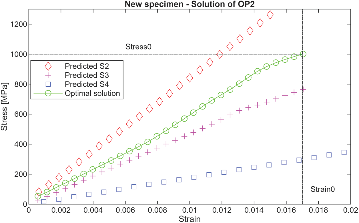
Figure 5: The stress-strain curve for OP2’s optimal solution (a = 26.43) and for the other laminates
Obviously, the OP2 might have different input data, such as S0 = 900.00 MPa. In this case, the optimization framework provides the following solution:
Optimal a = 27.87°; J0 = 1.136868e−13; S0 = 900.00 MPa.
The optimal orientation: 27.87/−27.87/.../27.87/−27.87/
Call count to PCM = 4320.
General aspects concerning the utilization of the OFW
Our work is placed in two scientific fields: (1) materials science, and (2) AI, represented by ML–regression models and metaheuristic algorithms like PSO. Each one has its own theoretical and practical distinct background. This paper is the continuation of a research work whose results were communicated in [2]. Roughly, [2] is a simulated study that gives some directions towards the construction of ML regression models for a family of composite laminates. Here, aspects related to materials science were largely presented and discussed. The model RNN2, which has a good generalization accuracy, was taken over for this study. As we mentioned in the Introduction section, our main objective was to answer a question: Can this prediction tool be used to find the combination of orientations (angles) that optimizes an objective function? Let’s note that RNN2 is implicitly “specialized” on the family of CLs.
We have proved that the answer is positive using two constructions:
▪ An optimization framework (OFW) with two modules, AHTPSO and the PCM.
▪ Two OPs concerning the orientations of the CLs have been proposed
Concerning the utilization of our work’s results, it is important to notice:
1. The optimization framework (OFW) has a general character; specialists in CMs can use it to solve their own problems. To do this, they can change the ML regression model to be appropriate for the new problem.
2. Because this work is a simulation study, the problems OP1 and OP2 have been defined and solved to show how the OFW can be used and prove its effectiveness.
3. Solving another OP is possible after developing an ML regression model adequate to the new problem. RNN2 covers only the OPs concerning the family of CLs presented in [2] and this article. If the specialist in CMs addresses an OP concerning another type of CM, they need to develop a new ML regression model, not necessarily an RNN, according to the new problem. This new regression model will make predictions within the new problem context.
Remark 2: Specialists in CMs could use the capabilities of OFW in solving OPs on the design of custom composites used for different purposes. If the new CM belongs to a family for which there exists an ML regressive model, this model will be used to solve the OP. Otherwise, a new regressive model must be constructed. This is not a simple task because the new model must embody the desired behavior of the new CM. The new model is not necessarily a stochastic model that predicts; it could also be a deterministic model (if any).
Remark 3: In the context of Remark 2, whatever the CM’s model would be, the success of finding optimal parameters mainly depends on the specialists in CM’s ability to formulate the OPs. They will determine what to minimize or maximize, which defines the objective function. Setting the problem constraints is equally important and can be critical in determining the computational complexity when solving the OP.
Implicitly, Remarks 2 and 3 reinforce the equal importance of the three components of an OP: the family model to which the object belongs, constraints related to the object’s properties, and the objective function. The formulation of OP1 serves as a good example from this perspective.
If we want to extend the use of the OFW to other material properties, other than fiber orientations, due to the systematic organization of OFW, this concerns only the modification of PCM. The steps to follow are:
▪ Develop another ML model for the same CLs family or a new family, which will be integrated into the PCM. This model will consider the new material properties involved in data points. It is the CM specialist’s responsibility to establish the material properties that are subject to optimization and to define the structure of the data points.
▪ Formulate the OP whose solution is relevant to the design procedure.
▪ Modify only the PCM to reflect the OP’s formulation, in all three components.
▪ Execute OFW to obtain the optimal solution.
Of course, the AHTPSO will support very minor modifications, which involve changing the values of certain parameters during initialization (that can be interactive). The program is not modified.
Remark 2 stated that the new model can be a deterministic one capable of expressing the desired behavior of the CM. This will perhaps be the topic of a new research project.
The general structure of the PCM
Examining the structure of the two PCMs, we find that we can define fixed parts and even a fixed order of their internal tasks.
The PCM function has the important task of predicting the stress value based on the strain and other parameters used in the regression model RNN2. For this type of application involving composite laminates, regardless of the objective function, employing an RNN model involves two specific tasks:
• A data point is “assembled” corresponding to the current candidate solution, in order to harness the RNN.
• The call of the prediction method associated with the RNN object, to obtain the stress value.
For this reason, the two PCM functions, JXRefCurve and JFixPoint, both include instructions #5 and #6 that perform the two tasks. This remains true regardless of the objective function (the nature of the problem). The presence of these two tasks is a common feature of the PCM.
The tasks of the PCM are fixed and have a fixed order. Examining the structure of the two PCM functions, it results in the following sequential tasks:
1. Prepare the call of the prediction method.
2. Make the prediction.
3. Treatment of the problem’s constraints (if any).
4. Computation of the objective function value, J, for the current candidate solution.
5. Return J and the other values of interest.
This list is a kind of template for the PCM that can be used by the user when solving their own OPs.
The optimal solution curves for OP1 and OP2 are distinct.
Figs. 4 and 5 display the optimal solution curves for OP1 and OP2, respectively. Both curves—optimal solution curves 1 and 2—reach the same endpoint, (Strain0, 1000). For OP1, the constraint is
However, the two curves differ, even though they start and end at the same points, (0, 0) and (Strain0, 1000), respectively. Fig. 6 shows the difference between optimal solution curves 2 and 1, indicating that optimal solution curve 2 is mostly above 1.
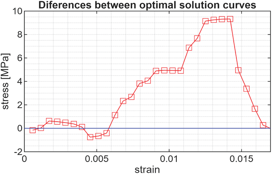
Figure 6: The “distance” between the optimal solution curves 2 and 1
Statistics of the OFW’s stochastic solutions
To explain the different quantitative behavior of the program implementing the optimization framework, we need to remember its stochastic nature. For example, running the program 30 times for solving OP1 produces 30 slightly different values of the performance index J0.
The minimum, average, maximum and typical values and standard deviation for the performance index J0 are given in the first line of Table 1. Another fact that illustrates the stochastic nature of the optimization framework is the call count for the function implementing PCM. The latter integrates the computation of the optimum criterion. The statistics for this number, Ncalls, are shown in the second line of Table 1 for the same 30 runs.
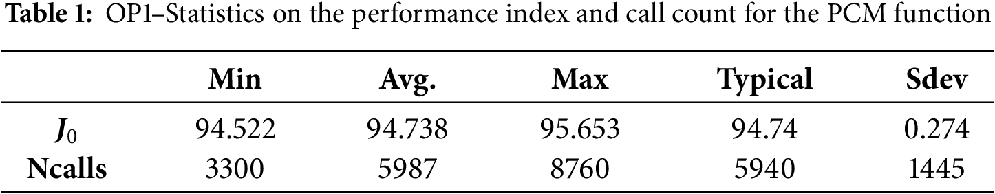
The typical value from a batch of 30 runs is the one nearest to the average value. The latter does not refer to a specific execution but is a result of mediation. The standard deviation of Ncalls is quite large because the swarm’s initialization has the simplest implementation, which means selecting 30 particles—vectors with 8 elements–using a uniform random distribution within the research domain [20, 30]8.
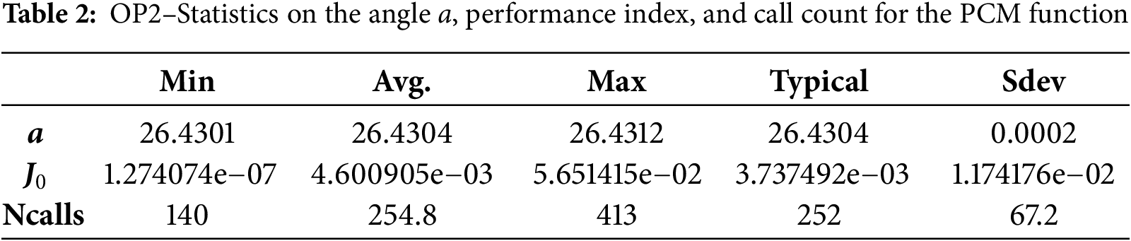
Regarding OP2, we initially used a large swarm of 30 particles, which produced the results shown earlier. The solution’s precision is so high that the performance index hits the lowest number the arithmetic processor can represent. To obtain a very good solution in a very short execution time, we considered in our simulations only 7 particles. Table 2 summarizes the results yielded in 30 runs of the program implementing the optimization framework.
Other optimization problems derived from OP2
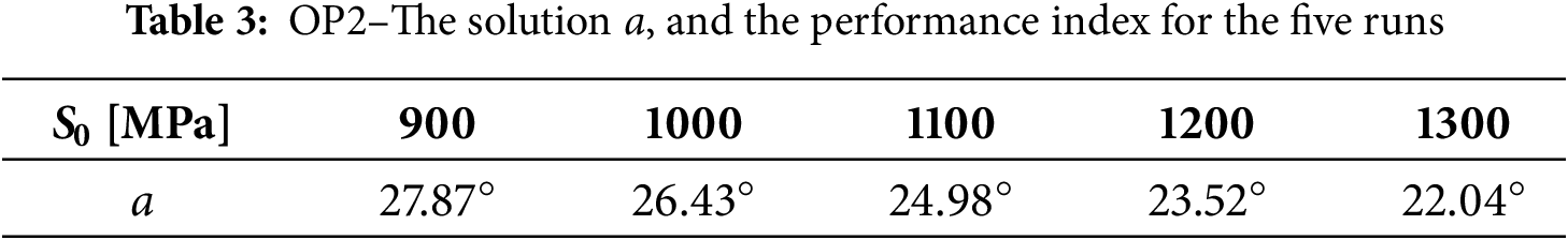
OP2 has been solved for different imposed values of S0 at the considered Strain0, using the same composite laminate modeled by RNN2. The values of S0 were chosen to span the range between S2 and S3, specifically 900, 1000, 1100, 1200, and 1300 MPa. The five runs with a large swarm (30 particles) produced the curves shown in Fig. 7.
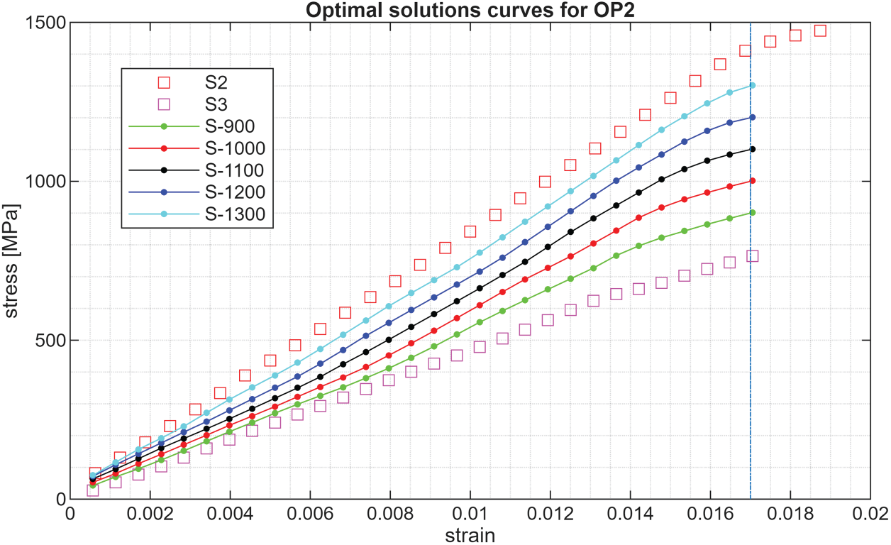
Figure 7: Optimal solution curves for OP2 and different values of S0
The solutions are given in Table 3, which provides the angle a.
Limitations of using OFW
Our simulation results proved that the two case studies can be treated efficiently. Certainly, the effectiveness of the search mechanism is crucial, and PSO offers versions that perform well in solving the OP. However, this is only part of the problem. The other part involves the accuracy and the generalization power of the ML regression model. The designer of this optimization framework must ensure the use of a regression algorithm with strong generalization capacity. In our opinion, this is the key point of our approach.
The ML model has good generalization power when used properly, meaning the specimens are within the model representation domain. The latter is not always so large as we would need. If we consider specimens outside the representation domain of the model, the predictions may have unacceptable errors. This is the main limitation of the proposed optimization approach, and it isn’t easy to deal with. In our case, the RNN2 has been shown to have good generalization power for the considered specimens [2]. However, there is generally no way to verify if this condition is strictly met. Depending on the dataset and the practical application, the user can a priori assume a specific representation domain of the model, and check through tests and simulations whether their hypothesis is correct.
This work demonstrates that the layer orientations of composite laminates, belonging to a specific class, can be determined by solving an optimization problem. The latter is solved through collaboration between the AHTPSO and an RNN. The AHTPSO ensures an efficient search mechanism, while the RNN serves as the regressive model for stress-strain dependence, obtained through an ML algorithm.
To organize the communication between the two components, an optimization framework was proposed that allowed us to give a systematic character to this collaboration. The AHTPSO algorithm deals with finding optimal solutions, while the PCM performs all tasks that define the OP (prediction, constraints checking, and cost function calculation).
This work is a simulation study that formulated two OPs to show that the optimization framework can solve them efficiently. The implementation of the OFW is achieved in MATLAB R2025b. Despite their stochastic and approximative nature, the solutions are very accurate and achieved with very acceptable computational complexity.
The limitation of using the proposed OFW is the quality of the ML model. The stress-strain dependences of the new specimens involved in the optimization process must be within the representation domain of the RNN model. Only in this way does the RNN achieve good generalization ability.
The OFW introduced in this work provides important insights that extend its applicability.
• Besides AHTPSO, other metaheuristic algorithms can be adapted to the proposed framework, such as evolutionary algorithms.
• Instead of an RNN model, another type of ML model can be used as a predictor if it provides highly accurate predictions and good generalization ability for the candidate specimens.
• The OFW can be applied to different types of problems, where predictions can accurately replace the system’s physical states. The specialist in CMs must develop a new ML regression model in line with the new family of CMs and the targeted material properties.
The authors’ future work is aimed at these possible extensions. First, solving the same problems with different metaheuristics or ML models will allow comparisons between solutions.
Acknowledgement: Thanks to the project team colleagues for their valuable comments on the work.
Funding Statement: This research was supported by the Ministry of Research, Innovation and Digitization, CNCS/CCCDI–UEFISCDI (Romania), Nr. 11/2024, within PNCDI IV. The APC received no external funding.
Author Contributions: The authors confirm contribution to the paper as follows: Conceptualization, Viorel Mînzu; methodology, Viorel Mînzu; software, Viorel Mînzu, Iulian Arama; validation, Iulian Arama; formal analysis, Viorel Mînzu; investigation, Viorel Mînzu; resources, Iulian Arama; data curation, Iulian Arama; writing—original draft preparation, Viorel Mînzu; writing—review and editing, Viorel Mînzu, Iulian Arama; visualization, Iulian Arama; supervision, Viorel Mînzu; project administration, Viorel Mînzu; funding acquisition, Iulian Arama. All authors reviewed the results and approved the final version of the manuscript.
Availability of Data and Materials: Not applicable.
Ethics Approval: Not applicable.
Conflicts of Interest: The authors declare no conflicts of interest to report regarding the present study.
Abbreviations
| ML | Machine Learning |
| CL | Composite Laminate |
| RNN | Regression Neural Network |
| OFW | Optimization Framework |
| OP | Optimization Problem |
| PSO | Particle Swarm Optimization |
| AHTPSO | Adaptive Hybrid Topology PSO |
| PCM | Prediction and Computation Module |
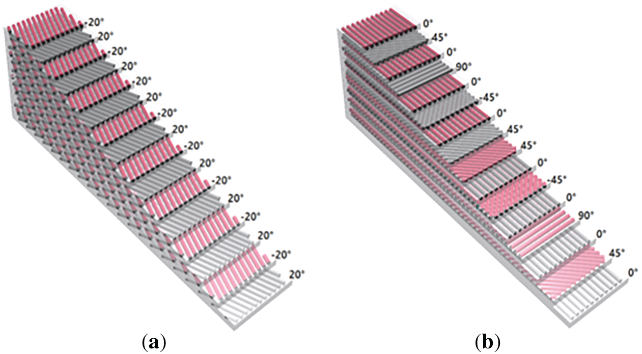
Figure A1: Two CL specimens: (a) Off-axis oriented specimen; The sequence [20°/−20°] is repeated. (b) Symmetrically balanced specimen. The sequence [0°/45°/0°/90°/0°/−45°/0°/45°] is repeated symmetrically
Characteristics of the RNN2 model
The application Regression Learner from MATLAB, using the Bayesian optimizer, found the best hyperparameter values:
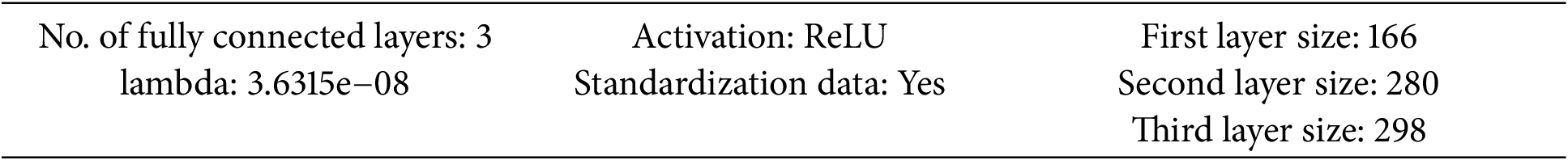
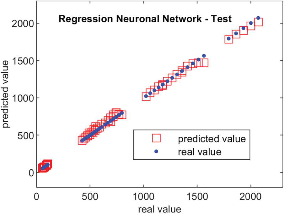
Figure A2: Comparison of actual and predicted values during RNN2 test phase
References
1. Liang Y, Wei X, Peng Y, Wang X, Niu X. A review on recent applications of machine learning in mechanical properties of composites. Polym Compos. 2025;46(3):1939–60. doi:10.1002/pc.29082. [Google Scholar] [CrossRef]
2. Ben Brayek BE, Sayed S, Mînzu V, Tarfaoui M. Machine learning predictions for the comparative mechanical analysis of composite laminates with various fibers. Processes. 2025;13(3):602. doi:10.3390/pr13030602. [Google Scholar] [CrossRef]
3. Vahed R, Zareie Rajani HR, Milani AS. Can a black-box AI replace costly DMA testing? —A case study on prediction and optimization of dynamic mechanical properties of 3D printed acrylonitrile butadiene styrene. Materials. 2022;15(8):2855. doi:10.3390/ma15082855. [Google Scholar] [PubMed] [CrossRef]
4. Kibrete F, Trzepieciński T, Gebremedhen HS, Woldemichael DE. Artificial intelligence in predicting mechanical properties of composite materials. J Compos Sci. 2023;7(9):364. doi:10.3390/jcs7090364. [Google Scholar] [CrossRef]
5. Ho NX, Le TT, Le MV. Development of artificial intelligence based model for the prediction of Young’s modulus of polymer/carbon-nanotubes composites. Mech Adv Mater Struct. 2022;29(27):5965–78. doi:10.1080/15376494.2021.1969709. [Google Scholar] [CrossRef]
6. Nneji RI, Nneji GU, Monday HN, Olumba WC, Agbonifo D, David GM, et al. Ensemble machine learning approaches to predicting mechanical properties of carbon fiber reinforced composites. World Sci News. 2024;197:158–81. doi:10.33599/nasampe/c.24.0245. [Google Scholar] [CrossRef]
7. Pathan MV, Ponnusami SA, Pathan J, Pitisongsawat R, Erice B, Petrinic N, et al. Predictions of the mechanical properties of unidirectional fibre composites by supervised machine learning. Sci Rep. 2019;9(1):13964. doi:10.1038/s41598-019-50144-w. [Google Scholar] [PubMed] [CrossRef]
8. Huang P, Dong JC, Han XC, Qi YP, Xiao YM, Leng HY. Prediction of mechanical properties of composite materials based on convolutional neural network-long and short-term memory neural network. Metalurgija. 2024;63:369–72. [Google Scholar]
9. Prada Parra D, Ferreira GRB, Díaz JG, de Castro Ribeiro GM, Braga AMB. Supervised machine learning models for mechanical properties prediction in additively manufactured composites. Appl Sci. 2024;14(16):7009. doi:10.3390/app14167009. [Google Scholar] [CrossRef]
10. Yang C, Kim Y, Ryu S, Gu GX. Prediction of composite microstructure stress-strain curves using convolutional neural networks. Mater Des. 2020;189:108509. doi:10.1016/j.matdes.2020.108509. [Google Scholar] [CrossRef]
11. Goodfellow I, Bengio Y, Courville A. Machine learning basics. In: Deep learning. Cambridge, MA, USA: The MIT Press; 2016. p. 96–161. [Google Scholar]
12. Goodfellow I, Bengio Y, Courville A. Example: linear regression. In: Deep learning. Cambridge, MA, USA: The MIT Press; 2016. p. 104–13. [Google Scholar]
13. Newbold P, Carlson WL, Thorne B. Multiple regression. In: Pfaltzgraff M, Bradley A, editors. Statistics for business and economics. 6th ed. Upper Saddle River, NJ, USA: Pearson Education, Inc.; 2007. p. 454–537. [Google Scholar]
14. The MathWorks Inc. Stepwise regression toolbox documentation, Natick, Massachusetts [Internet]. 2024 [cited 2026 Jan 5]. Available from: https://www.mathworks.com/help/stats/stepwise-regression.html. [Google Scholar]
15. The MathWorks Inc. Regression Neural Network Toolbox Documentation, Natick, Massachusetts [Internet]. 2024 [cited 2026 Jan 5]. Available from: https://www.mathworks.com/help/stats/regressionneuralnetwork.html. [Google Scholar]
16. Clerc M. L’optimisation par essaims particulaires-versions paramétriques et adaptatives. Paris, France: Hermès Science; 2005. (In French). [Google Scholar]
17. Feng L, Ge Y, Gao L. Self-adaptive particle swarm optimization algorithm for global optimization. In: Proceedings of the 2010 Sixth International Conference on Natural Computation; 2010 Aug 10–12; Yantai, China. doi:10.1109/ICNC.2010.5582543. [Google Scholar] [CrossRef]
18. Beheshti Z, Shamsuddin SM, Sulaiman S. Fusion global-local-topology particle swarm optimization for global optimization problems. Math Probl Eng. 2014;2014(1):907386. doi:10.1155/2014/907386. [Google Scholar] [CrossRef]
19. Beheshti Z, Shamsuddin SM, Hasan S. Memetic binary particle swarm optimization for discrete optimization problems. Inf Sci. 2015;299:58–84. doi:10.1016/j.ins.2014.12.016. [Google Scholar] [CrossRef]
20. Minzu V, Barbu M, Nichita C. A Binary Hybrid Topology Particle Swarm Optimization algorithm for sewer network discharge. In: Proceedings of the 2015 19th International Conference on System Theory, Control and Computing (ICSTCC); 2015 Oct 14–16; Cheile Gradistei, Romania. doi:10.1109/ICSTCC.2015.7321363. [Google Scholar] [CrossRef]
21. Valadi J, Siarry P. Applications of metaheuristics in process engineering. London, UK: Springer; 2014. doi:10.1007/978-3-319-06508-3. [Google Scholar] [CrossRef]
22. Mînzu V, Arama I. A machine learning algorithm that experiences the evolutionary algorithm’s predictions—an application to optimal control. Mathematics. 2024;12(2):187. doi:10.3390/math12020187. [Google Scholar] [CrossRef]
23. Mînzu V, Arama I, Rusu E. Machine learning algorithms that emulate controllers based on particle swarm optimization—an application to a photobioreactor for algal growth. Processes. 2024;12(5):991. doi:10.3390/pr12050991. [Google Scholar] [CrossRef]
Cite This Article
 Copyright © 2026 The Author(s). Published by Tech Science Press.
This work is licensed under a Creative Commons Attribution 4.0 International License , which permits unrestricted use, distribution, and reproduction in any medium, provided the original work is properly cited.
 Downloads
 Citation Tools