Machine Learning-Driven Prediction of the Glass Transition Temperature of Styrene-Butadiene Rubber

1  Introduction

Styrene-butadiene rubber (SBR) is the most widely produced synthetic rubber in the world. Its copolymer structure of styrene and butadiene in the molecular chain gives the material excellent wear resistance, anti-slip properties, and processing performance, making it indispensable in tyre manufacturing, shock-absorbing materials, industrial seals, and other fields [1]. However, there is a complex nonlinear relationship between the macro performance of SBR and its multi-level, multi-tiered microstructure. Among these, Tg is a core parameter that characterises the mobility of polymer chains and directly determines the material’s low-temperature flexibility and dynamic mechanical properties [2]. Traditional Tg prediction methods mainly rely on empirical formulas such as the Flory-Fox equation and the Gordon-Taylor equation [3,4]. These methods are based on the linear addition assumption and have significant limitations in characterising microscopic factors such as copolymer segment synergistic effects and topological structures [3,4]. In recent years, molecular dynamics (MD) simulations have provided a new approach to predicting the Tg of polymers through conformational energy barrier calculations [5]. However, MD simulations face challenges such as time scale limitations, inaccurate force field parameterisation, and high computational costs when predicting Tg [6,7]. For example, David et al. predicted the Tg of polyethylene through molecular dynamics simulations and found that different fitting ranges could result in Tg values varying by as much as 70 K, exposing the inherent limitations of molecular dynamics simulation methods [8]. Against this backdrop, establishing a quantitative mapping relationship between the microstructure of SBR and its Tg, and achieving precise prediction and targeted regulation of the Tg of SBR, has become a critical scientific issue in SBR material design and performance optimisation.

In recent years, machine learning (ML) technology has been widely applied in various fields of scientific research, and its emergence and application in the field of polymer materials has provided new solutions to the above problems [9]. Compared with traditional empirical models, machine learning, with its non-linear modelling advantages, can effectively construct multi-variable, non-linear polymer material structure-property relationships, enabling accurate prediction of material properties [10,11]. Machine learning has made significant progress in predicting the properties of polymer materials. For example, Zhang et al. used an artificial neural network model to accurately predict Tg of polyimide, with an average deviation of only 3.66% between the model predictions and experimental results [12]. Ding et al. successfully achieved precise prediction of the mechanical properties of polyurethane elastomers with complex chemical structures using the extreme gradient boosting tree (XGBoost) algorithm, with the model’s R2 value reaching 0.91 [13]. Liu et al. developed an extreme learning machine (ELM) model to achieve high-precision prediction of the fatigue life of natural rubber, with the model’s accuracy improved by 10% compared to traditional algorithms. These studies confirm that machine learning demonstrates strong modelling capabilities and engineering application potential in the prediction of polymer material properties [14]. However, research on the application of machine learning in predicting Tg of SBR faces challenges such as the difficulty of traditional linear regression algorithms in capturing the nonlinear relationship between SBR structure and Tg [15].

In response to the aforementioned challenges, this study proposes a machine learning-based framework for predicting the Tg of SBR. A machine learning prediction model framework suitable for multi-component SBR systems was established. The performance of nine machine learning algorithms was systematically investigated, and a GPR-XGBoost mixed prediction model was further constructed through model ensemble to enhance the model’s generalisation capability and prediction accuracy. Additionally, interpretability analysis methods such as SHAP and ALE are introduced to deeply explore the mechanisms by which different components influence Tg, aiming to provide effective theoretical tools and technical pathways for the structural design and performance regulation of SBR. This study not only provides an efficient tool for predicting the Tg of SBR but also offers methodological references for performance prediction in other copolymer systems.

2  Data and Methods

2.1 Data Collection and Processing

We collected data on the structure and Tg of SBR from various published papers in databases such as Web of Science and China National Knowledge Infrastructure (CNKI) [16–19]. The data screening criteria were set as follows: (1) the samples were pure SBR copolymers, excluding mixed systems containing third monomers; (2) the monomer composition content (styrene and butadiene isomer ratio) of SBR is determined by standard 1H-NMR or Fourier transform infrared spectroscopy techniques. Tg was measured using differential scanning calorimetry (DSC) at a standard heating rate (10–20°C/min); (3) The content of styrene and butadiene isomers was explicitly provided. After data screening, we constructed an SBR dataset comprising 96 sample data sets, covering styrene, 1,2-butadiene, cis-1,4-butadiene, and trans-1,4-butadiene content and their corresponding Tg values. Styrene, 1,2-butadiene, cis-1,4-butadiene, and trans-1,4-butadiene content were used as feature variables, and Tg was the target variable. The rationale for selecting these four features lies in the chemical nature of SBR. As a copolymer, the Tg of SBR is fundamentally determined by the ratio of styrene to butadiene and the isomeric configuration of the butadiene units (1,2-butadiene, cis-1,4-butadiene, and trans-1,4-butadiene). These four components constitute the complete microstructure of the polymer chains, directly governing chain flexibility and intermolecular interactions. This provided sufficient data support for subsequent model training.

Based on the collected data, the dataset was divided into a training set (n = 72) and a test set (n = 24) at a ratio of 3:1. The distribution of the complete dataset and the data distribution of the training set and test set are shown in Fig. 1. It can be seen that the training set and test set retain the overall data distribution well, so the dataset division is considered reasonable. The complete dataset is presented in Table S1 for further reference.

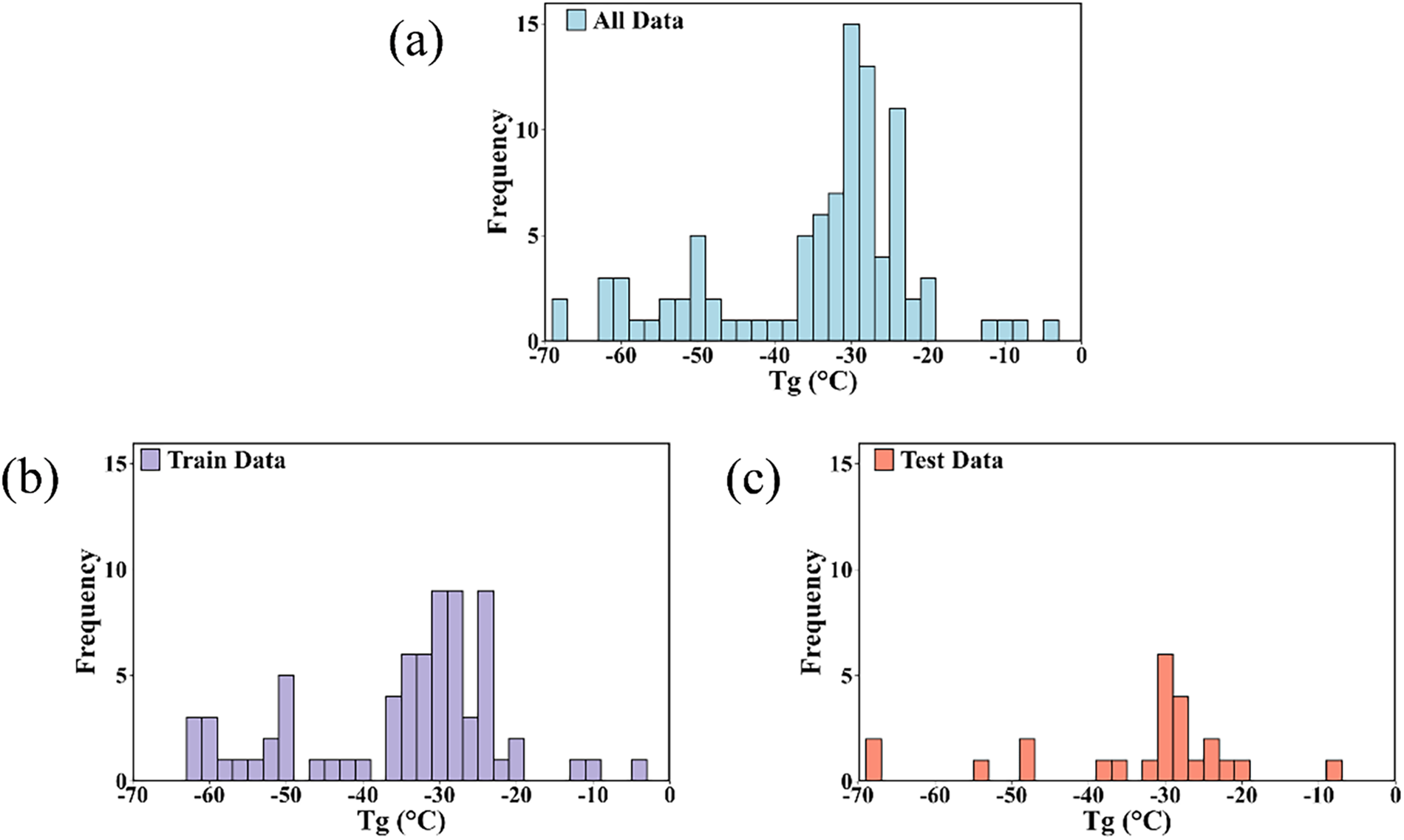
Figure 1: (a) Distribution of complete data sets; (b) Data distribution of the training set; (c) Data distribution of the test set

2.2 Machine Learning Algorithms

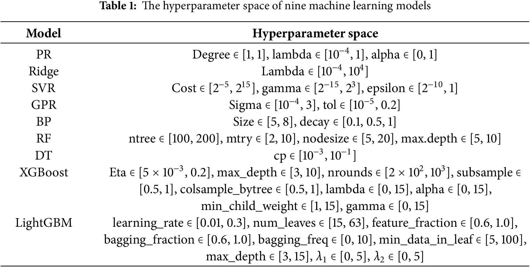
Through literature review, this study adopted the nine most commonly used algorithms for further research. These nine algorithms can be divided into four types: regression algorithms, kernel algorithms, neural networks, and tree-based algorithms. Different machine learning algorithms were used to learn, train, and optimise the data in the constructed database, resulting in machine learning models based on different algorithms. The best prediction model was then selected to achieve high-precision prediction of Tg of SBR. The hyperparameter spaces employed for the nine models in this study are presented in Table 1.

2.2.1 Regression Algorithms

Polynomial Regression (PR): The PR algorithm constructs a non-linear regression model by introducing higher-order terms (such as quadratic and cubic terms) of feature variables to capture the non-linear relationship between input variables and output. Essentially, it converts non-linear problems into linear fits in high-dimensional spaces by increasing the feature dimension. This algorithm has a simple structure and high computational efficiency, making it suitable for modelling moderately complex non-linear relationships [15].

Ridge Regression (Ridge): The Ridge algorithm introduces an L2 regularisation term based on linear regression, reducing the risk of overfitting by constraining the size of the model coefficients and improving the stability of the model. Its advantages lie in its ability to handle high-dimensional data and alleviate multicollinearity issues, making it suitable for datasets where the number of features far exceeds the number of samples or where there are strong correlations [20,21].

2.2.2 Nuclear Algorithms

Support Vector Machine Regression (SVR): SVR is based on the principle of minimising structural risk. It uses kernel functions to map data to a high-dimensional space and finds the hyperplane that maximises the number of samples within the error band to establish a regression model, thereby handling linear and non-linear regression problems. SVR has strong generalisation capabilities for small samples and high-dimensional data and is resistant to noise interference, but its computational complexity increases significantly with the number of samples [22].

Gaussian Process Regression (GPR): GPR is based on the assumption that data follows a Gaussian distribution. It uses kernel functions to describe the similarity between samples and outputs the probability distribution of predicted values. Its main feature is that it can provide uncertainty intervals for prediction results. However, its computational complexity increases significantly with the amount of data, making it suitable for small-scale continuous data where confidence intervals need to be quantified [23,24].

2.2.3 Backpropagation Neural Network (BP)

BP is an algorithm based on artificial neural networks that extracts data features step by step through a multi-layer neuron structure, combining non-linear activation functions with backpropagation algorithms to optimise weight parameters. This model can fit highly complex non-linear relationships, but it is prone to getting stuck in local optima and is sensitive to noise in the training data [25].

2.2.4 Algorithms Based on Tree Models

Decision Tree (DT): DT generates a tree model by recursively partitioning the feature space. Each internal node represents a feature, and the leaf nodes represent the predicted values. Decision trees are simple and easy to understand, and can handle classification and regression tasks, but they are prone to overfitting and have poor generalisation capabilities [26,27].

Random Forest (RF): RF is an ensemble learning algorithm based on decision trees. It integrates multiple decision trees and uses a voting mechanism to enhance model stability. Its strategy of randomly sampling features and samples enhances its generalisation ability. This algorithm has excellent noise resistance and stability, making it suitable for processing datasets with high-dimensional features [28].

Extreme Gradient Boosting (XGBoost): XGBoost is an algorithm based on gradient boosting trees, which iteratively optimises weak classifiers based on gradient boosting trees and balances bias and variance through regularisation terms and weighted loss functions. Its advantages include fast data training speed and the ability to efficiently process large-scale data [29].

Lightweight Gradient Boosting Machine (LightGBM): LightGBM is an efficient gradient boosting algorithm that improves the node splitting strategy of gradient boosting trees, uses histogram algorithms to compress feature values, and implements one-sided gradient sampling to reduce computational load. This method has significant advantages in terms of memory usage and training speed, and is suitable for non-linear modelling tasks involving large-scale data.

2.3 Bayesian Optimisation

Common hyperparameter optimisation methods used in machine learning modelling include: random search [30], grid search [31], and Bayesian optimisation [32]. This study employs Bayesian optimisation for hyperparameter tuning. Compared to random search, Bayesian optimisation typically converges 3–5 times faster, enabling more efficient reduction of ineffective trials. While grid search is more thorough, its computational complexity grows exponentially with dimension and requires traversing a large number of parameter combinations. Bayesian optimisation, however, uses Gaussian process surrogate models for search, enabling efficient identification of optimal hyperparameters in high-dimensional feature spaces [33].

The principle of Bayesian optimisation is as follows: first, select a set of initial points {x1,x2,…xn} and calculate the objective function value f(xi) at these points to obtain the initial observation data set:

D={(xi,f(xi))}i=1n(1)

Subsequently, a Gaussian process (GP) is modelled based on dataset D to obtain the predicted distribution of the objective function, which takes the form:

P(f(x∗)∣x∗,D)=N(μ(x∗,σ2(x∗))(2)

Among them, the predicted mean and predicted variance are as follows:

μ(x∗)=k∗T(K+σn2I)−1y(3)

σ2(x∗)=k(x∗,x∗)−k∗T(K+σn2I)−1k∗(4)

Here, k is the kernel function, K is the kernel matrix of the training samples, k∗ is the kernel vector of the test point and training samples, and σn2 is the observed noise variance.

After obtaining the predicted distribution, introduce the acquisition function a(x∣D) to balance exploration and exploitation. Select the next sampling point by maximising the acquisition function:

xn+1=arg⁡maxa(x∣D)(5)

At this point, perform a true evaluation of the objective function f(xn+1) and add the new observation data point (xn+1,f(xn+1)) to the data set D. Repeat the above process until the predefined termination condition is met [34].

2.4 Model Evaluation

Using a unified set of evaluation metrics is key to fairly comparing the predictive performance of different models. By relying on these metrics, we can determine whether a model accurately captures the characteristics of a dataset when fitting existing data, and further assess whether the model can be effectively generalised to unknown data of the same type. The coefficient of determination (R2), root mean square error (RMSE), and mean absolute error (MAE) are commonly used to evaluate the overall predictive performance of a model. In this study, these metrics were used to evaluate the predictive accuracy of each model, with their expressions as follows:

R2=1−∑i=1n(yi−yi^)2∑i=1n(yi−yi¯)2(6)

RMSE=1n∑i=1n(yi−yi^)2(7)

MAE=1n∑i=1n|yi−yi^|(8)

Here, yi, yi¯, and yi^ represent the actual value, the mean of the actual values, and the predicted value, respectively. RMSE and MAE are used to evaluate prediction errors, with smaller values indicating better model fit. The theoretical range of R2 is [0, 1], with values closer to 1 indicating higher model prediction accuracy.

3  Results and Discussion

3.1 Prediction Results of Single Model

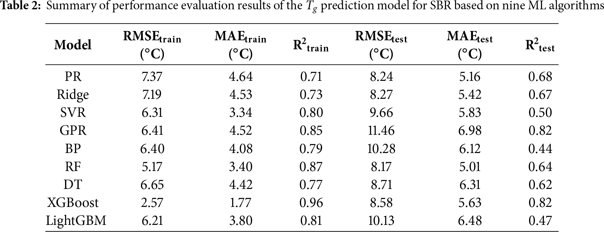
Fig. 2 shows the prediction results of nine machine learning algorithm models. The vertical axis depicts the model’s predicted values, while the horizontal axis reflects the actual values. Green points represent the training set, and red points represent the test set. The closer the data points are clustered around the diagonal line, the higher the model’s predictive accuracy. A comparison of model predictive performance is shown in Table 2. As can be seen from Fig. 2 and Table 2, the R2 values for the PR and Ridge models on the test set are 0.68 and 0.67, respectively, indicating that these two models have limited ability to capture the nonlinear relationship between SBR structural composition and corresponding Tg, and their overall predictive accuracy is generally poor. The SVR model has an R2 of 0.80 for the training set, but the R2 for the test set drops to 0.50, indicating poor generalisation ability and significant overfitting. This is because the SVR model is sensitive to regularisation parameters and is easily affected by local data perturbations, leading to weak generalisation ability; The GPR model, however, demonstrates better nonlinear fitting capability under small sample conditions through adaptive adjustment of kernel function parameters, achieving R2 values above 0.8 in both the training and test sets, indicating excellent generalisation capability and robustness. The BP model achieved an R2 of 0.79 on the training set, but the R2 on the test set dropped to 0.44, and the RMSE increased from 6.40 to 10.28, indicating obvious overfitting. This suggests that a single-hidden-layer network structure may not effectively balance model complexity and data scale. The XGBoost model performed the best among the four tree models, with an R2 of 0.96 and an RMSE of 2.57 on the training set; on the test set, it achieved an R2 of 0.82 and an RMSE of 8.58, significantly outperforming the other three tree models. Its advantage lies in its gradient boosting strategy and regularisation, which effectively correct prediction errors and significantly reduce model bias. Comparisons show that while RF, DT, and LightGBM perform reasonably well on the training set, their performance on the test set is poor, indicating that these three models exhibit significant overfitting and poor prediction accuracy.

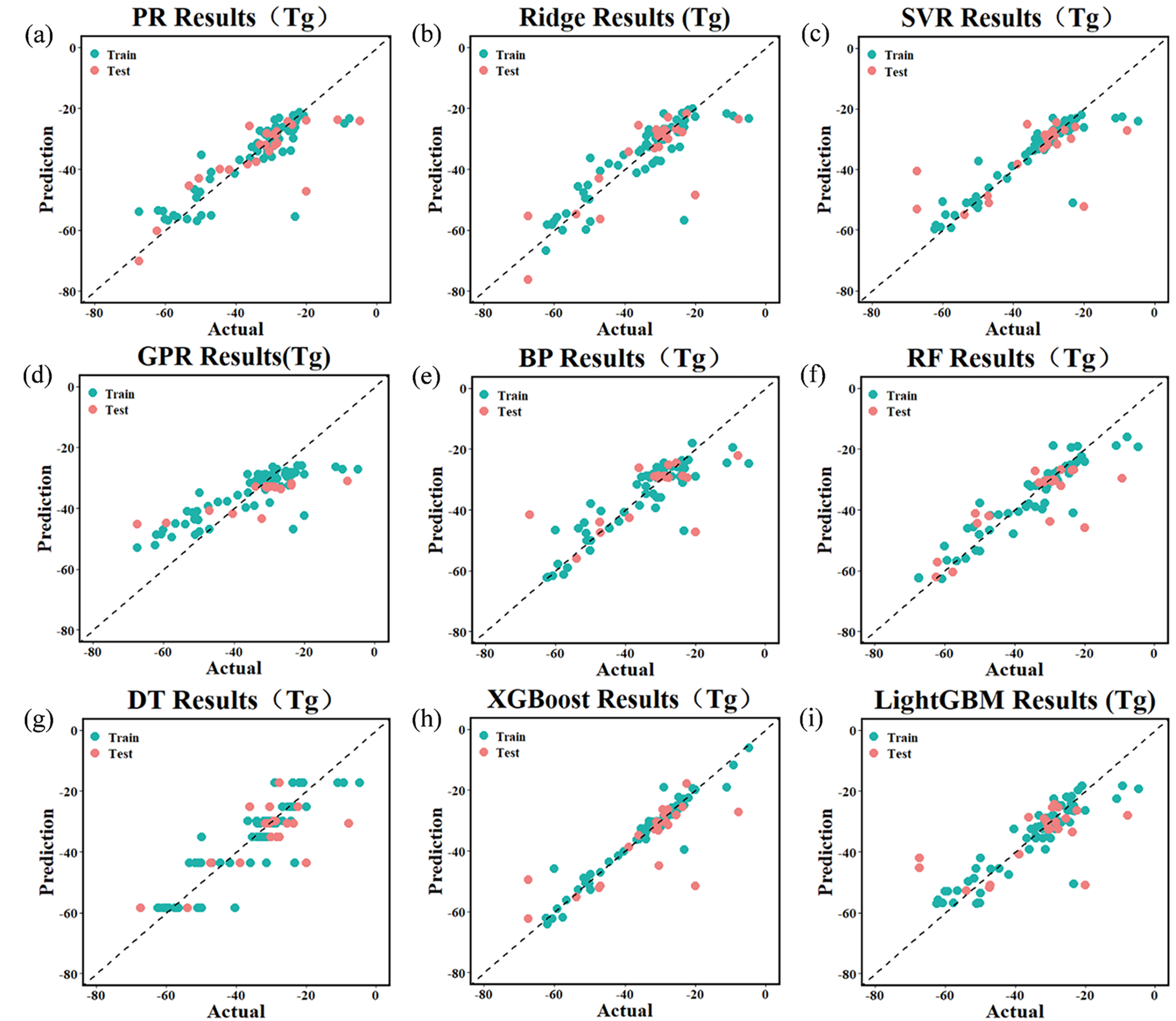
Figure 2: Prediction results of the Tg of SBR using different machine learning models: (a) PR model; (b) Ridge Regression model; (c) SVR model; (d) GPR model; (e) BP neural network model; (f) DT model; (g) RF model; (h) XGBoost model; (i) LightGBM model

Overall, both GPR and XGBoost models achieve R2 values above 0.8 on both the training and test sets. Among them, the GPR model demonstrates the best stability; the XGBoost model achieves the highest prediction accuracy but exhibits a certain degree of overfitting.

3.2 Prediction Results of the GPR-XGBoost Mixed Model

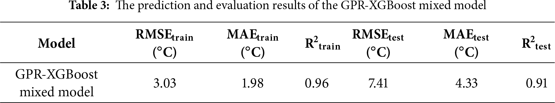
In the comparison of single model prediction results, the GPR model demonstrated the best stability; the XGBoost model achieved the highest prediction accuracy but exhibited a certain degree of overfitting. To further enhance the predictive performance of the models, the GPR model and XGBoost model were integrated to construct the GPR-XGBoost mixed model, with its prediction results shown in Fig. 3 and Table 3. The results show that the R2 of the GPR-XGBoost mixed model exceeds 0.9 in both the training set and the test set. Compared to the single GPR and XGBoost models, the R2 of the GPR-XGBoost mixed model is significantly improved, while the RMSE and MAE are significantly reduced; its overall predictive performance is significantly superior to that of the single models. The true and predicted Tg values of the training and testing samples are shown in Tables S2 and S3.

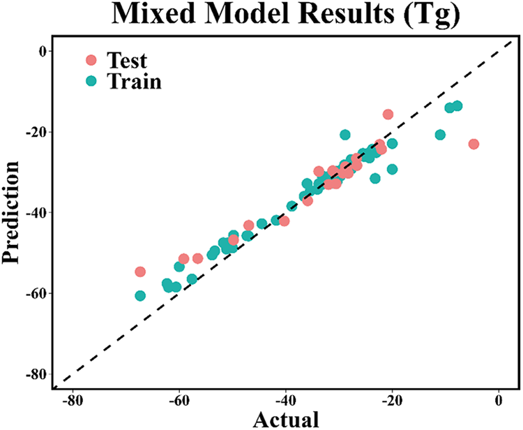
Figure 3: Taking the Tg of SBR as the prediction target, prediction results of the Tg of SBR using GPR-XGBoost mixed model

To enhance the model’s utility for industrial applications, we evaluated prediction reliability using 95% Prediction Intervals (PI). Unlike deterministic models, the GPR component of GPR-XGBoost mixed model allows for the quantification of predictive variance (σ2).

Fig. S1 and Fig. S2 respectively show the prediction intervals (95% confidence) of the training set samples and the test set samples using the GPR XGBoost mixed model. In Figs. S1 and S2, the blue dots represent the actual experimental values; The solid red line represents the predicted values generated by the GPR XGBoost hybrid model; The gray shaded area corresponds to 95% of the prediction interval (PI), reflecting the uncertainty range obtained by the GPR component.

The results show that the prediction interval coverage probability (PICP) of both the training and testing sets is high, and the predicted data points always fall within the calculated gray confidence interval. This confirms that the proposed GPR XGBoost hybrid model effectively captures random uncertainty, and its prediction accuracy has good reliability. It provides engineers with a dependable safety margin during the Tg prediction process for SBR.

3.3 Overfitting Test

To further assess the stability of the GPR, XGBoost, and GPR-XGBoost mixed models and determine the degree of overfitting for each model, we used 5-fold cross-validation to obtain the trends in R2 (represented as R-squared in the figure) for the GPR, XGBoost, and GPR-XGBoost mixed models in the training set and test set under different data volumes, as shown in Fig. 4. The results indicate that as the data volume increases, the XGBoost model remains stable in the training set with minimal fluctuations, but the results in the test set are significantly unstable, showing large fluctuations and inconsistent trends, indicating poor stability of the XGBoost model; meanwhile, the decision coefficient of the GPR model in the test set exhibits a stable upward trend as the data volume increases, indicating excellent stability of the GPR model; Additionally, compared to the XGBoost model, the stability of the GPR-XGBoost mixed model is significantly improved, indicating that the GPR-XGBoost mixed model combines the robustness of GPR with the high predictive accuracy of XGBoost, making it the optimal choice for predicting the Tg of SBR.

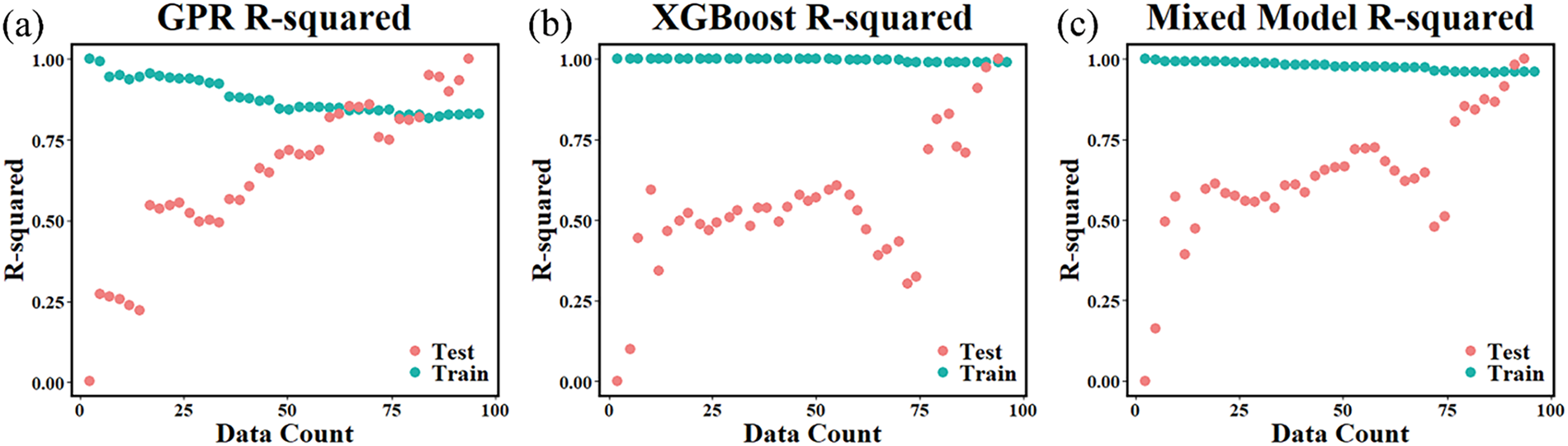
Figure 4: Taking the Tg of SBR as the prediction target, (a) GPR model; (b) XGBoost model (c) The determination coefficient of the GPR-XGBoost mixed model in the training set and the test set varies with the amount of data

3.4 Feature Analysis

3.4.1 Pearson Correlation Analysis

To analyse the relationship between the four feature variables and the target variable Tg, Pearson’s correlation coefficient was used for analysis, as shown in Fig. 5. This heatmap displays the Pearson correlation coefficients between the content of styrene, 1,2-butadiene, cis-1,4-butadiene, trans-1,4-butadiene, and Tg. The closer the coefficient is to 1, the stronger the correlation between the two variables. As shown in the Fig. 5, the correlation coefficient between Tg and 1,2-butadiene content is 0.76, indicating a strong positive correlation, meaning that as 1,2-butadiene content increases, Tg significantly rises; the correlation coefficient between Tg and trans-1,4-butadiene content is −0.68, indicating a strong negative correlation, meaning that as trans-1,4-butadiene content increases, Tg decreases. Additionally, the correlation coefficient between styrene content and Tg is 0.12, indicating a weak correlation. There are also varying degrees of correlation between the various characteristic variables. For example, the correlation coefficient between 1,2-butadiene and cis-1,4-butadiene content is −0.48, indicating a negative correlation. These correlation relationships help to understand the impact of changes in the content of various components of SBR on Tg, providing a reference and foundation for establishing a quantitative relationship between the content of various components of SBR and Tg.

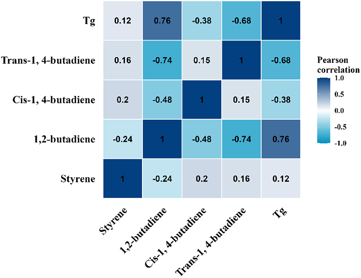
Figure 5: The Pearson correlation coefficient heat map between the four characteristic variables and the target variable

Although correlations exist between feature variables due to compositional constraints, dimensionality reduction techniques were not employed. Retaining the original feature space is crucial to preserve the physicochemical interpretability of the model, allowing for a direct mapping between specific microstructural elements and Tg. Furthermore, the GPR and XGBoost algorithms employed in this study possess intrinsic mechanisms to handle correlated predictors robustly.

3.4.2 Feature Importance Ranking

ML is essentially a ‘black box’ model lacking interpretability. To visually observe the influence of feature variables on both single models and ensemble models, the GPR model, XGBoost model, and GPR-XGBoost mixed model used for predicting the Tg of SBR were analysed based on a unified feature importance metric (Median Importance), with results shown in Fig. 6. As shown in Fig. 6a,b, the feature importance rankings for the GPR model and XGBoost model are identical: trans-1,4-butadiene > 1,2-butadiene > styrene > cis-1,4-butadiene. Fig. 6c shows that the feature ranking in the GPR-XGBoost mixed model exhibits minor changes, but the relative contributions of each feature are generally consistent with those of the GPR and XGBoost models. Overall, the content of 1,2-butadiene and trans-1,4-butadiene has the greatest influence on the Tg of SBR, while the content of styrene and cis-1,4-butadiene has a relatively smaller influence.

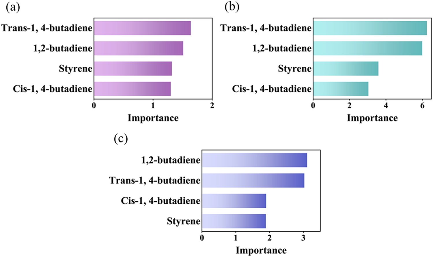
Figure 6: The ranking of feature importance of each model: (a) GPR model; (b) XGBoost model (c) GPR-XGBoost mixed model

The ranking results in Fig. 6 align well with polymer physics principles regarding chain flexibility and steric hindrance. Trans-1,4-butadiene and 1,2-butadiene are identified as the most critical features, reflecting their dominant roles in competing mechanisms that determine Tg. Physically, the 1,2-butadiene unit (vinyl structure) possesses bulky side groups that significantly increase steric hindrance and restrict the rotation of the main chain, thereby enhancing chain rigidity and raising Tg. In contrast, trans-1,4-butadiene offers a highly flexible linear backbone structure, which effectively lowers the energy barrier for segmental motion and reduces Tg. Furthermore, these features do not act in isolation but interact through a compositional constraint. Since the total content of the copolymer units sums to 100%, an increase in rigid components (e.g., 1,2-butadiene or styrene) inherently necessitates a decrease in flexible components (e.g., cis- or trans-1,4-butadiene). This relationship of one diminishing as the other increases constitutes strong interaction between features. The model determines which feature carries greater weight precisely by capturing this non-linear relationship of proportional change.

3.4.3 SHAP Analysis

The SHapley Additive exPlanations (SHAP) method is a widely used theoretical framework in machine learning model interpretability research. Its core idea is to quantify the importance of each input feature by calculating its marginal contribution to the prediction result. The resulting SHAP values can intuitively reflect the relative roles of different features in model predictions. In this study, we calculated and analysed the SHAP values of each input feature based on the XGBoost model to reveal their contribution to the prediction of Tg.

Fig. 7a shows the feature importance ranking determined by the average absolute values of the SHAP values of each feature variable. It can be seen that the content of 1,2-butadiene and trans-1,4-butadiene has the most significant effect on the Tg of SBR; the content of styrene has the second most significant effect, while the content of cis-1,4-butadiene has the least significant effect. Fig. 7b is a density scatter plot of the contributions of each feature variable to Tg. The wider areas in the figure indicate higher point density. The colour of the points indicates the magnitude of the feature values, with red representing high values and blue representing low values. When red scatter points are distributed on the side where the SHAP value is greater than 0, it indicates that the feature variable has a positive contribution to Tg. When blue scatter points are distributed on the side where the SHAP value is greater than 0, it indicates that the feature variable has a negative contribution to Tg. From Fig. 7b, it can be observed that the content of 1,2-butadiene and styrene has a positive contribution to Tg, while the content of trans-1,4-butadiene and cis-1,4-butadiene has a negative contribution to Tg. This is consistent with theoretical expectations.

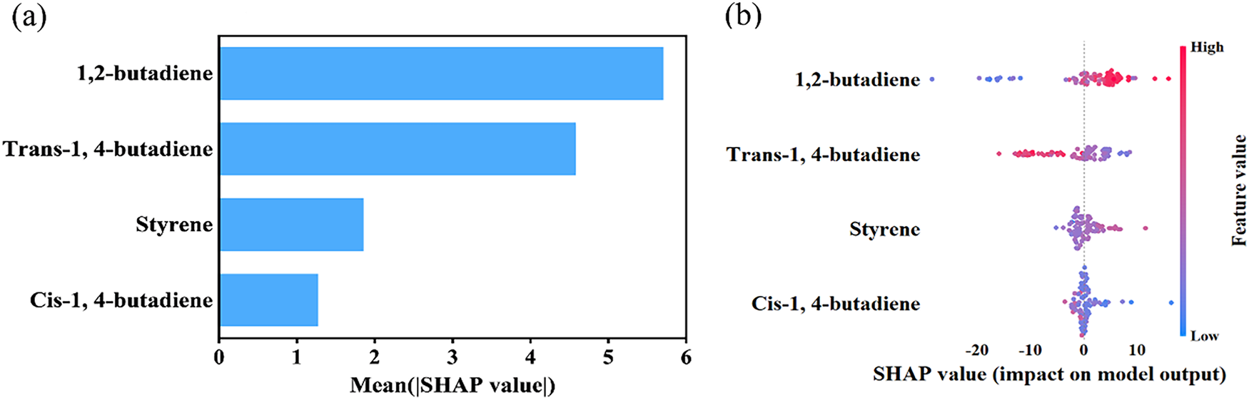
Figure 7: Taking the Tg of SBR as the prediction target, (a) the absolute average SHAP values of each characteristic variable to the prediction target; (b) The density scatter distribution map of the SHAP values of each characteristic variable for the predicted target

Generally, the flexibility of polymer chains determines Tg of polymers; the greater the flexibility of the polymer chains, the lower the Tg of the polymer [35,36]. 1,2-Butadiene has large side chains, and increasing the content of 1,2-butadiene enhances the rigidity of SBR molecular chains and intermolecular forces, thereby reducing the flexibility of the molecular chains and causing an increase in Tg [37]. An increase in styrene content also enhances the rigidity of SBR molecular chains and promotes the overlap and interaction of electron clouds between benzene rings, which restricts chain movement and leads to an increase in Tg [38]. The isolated double bonds in the cis-1,4-butadiene structure increase the rotational freedom of single bonds, enhancing the flexibility of polymer chains and resulting in a decrease in Tg. In contrast, in trans-1,4-butadiene, the substituents on either side of the double bond are located on opposite sides, resulting in a linear, zigzag arrangement of the main chain. The rotational freedom of the single bonds is extremely high, and the molecular chain flexibility is superior to that of the cis structure [39]. Therefore, an increase in trans-1,4-butadiene content leads to a more significant decrease in Tg.

3.4.4 ALE Analysis

Based on the aforementioned analysis, to delve deeper into the impact of features on Tg prediction and minimize the explanatory bias stemming from model dependency, we further employ Accumulated Local Effects (ALE) [40] to analyze the four feature variables in both the single model and the mixed model, as illustrated in Fig. 8. The horizontal axis represents the range of values for each feature, while the vertical axis indicates the accumulated local effect of that feature on the model’s prediction at each value point. This represents the average influence of the feature on the prediction output at its current value. To observe the impact of features on prediction results more clearly, we select regions with significant changes for plotting. This approach offers a more intuitive understanding of how features affect Tg prediction and aids in unveiling the nonlinear relationships and interactive effects between features and Tg, thereby enhancing the interpretability of the model.

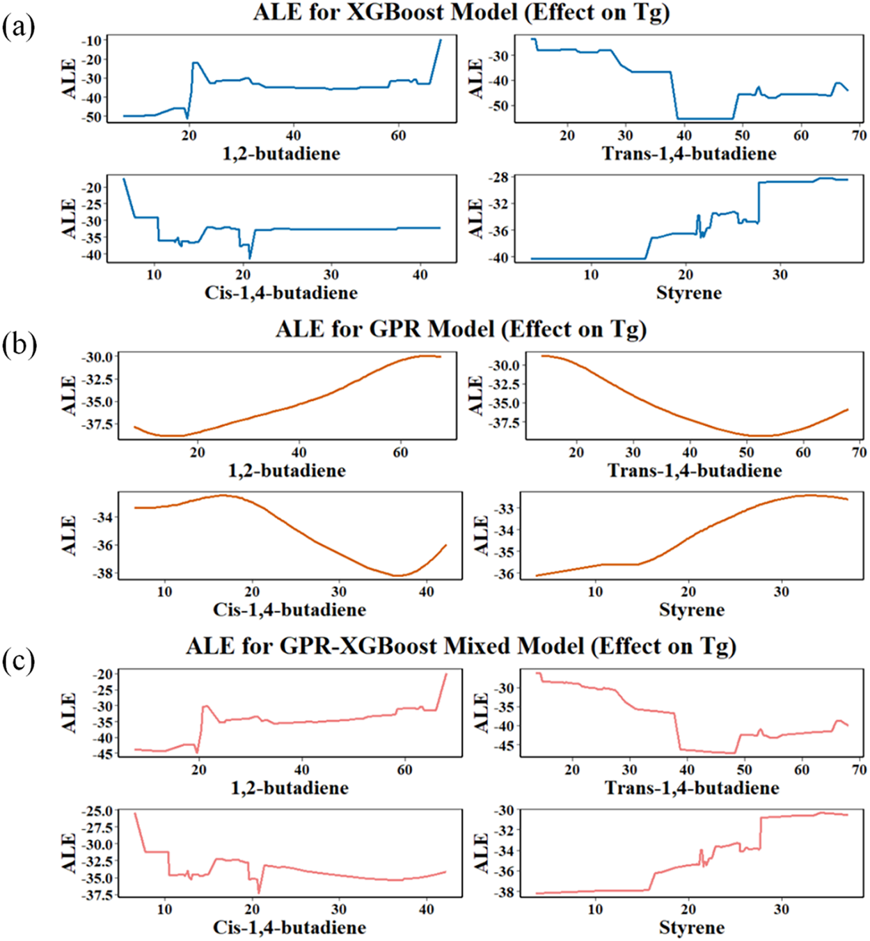
Figure 8: ALE analysis graphs of four characteristic variables in different models: (a) XGBoost model; (b) GPR model (c) GPR-XGBoost mixed model

As shown in Fig. 8, the content of 1,2-butadiene and styrene exhibits a positive effect on Tg in all three models, indicating that increasing the content of 1,2-butadiene and styrene is beneficial for enhancing the Tg of SBR. Conversely, the content of cis-1,4-butadiene and trans-1,4-butadiene in all three models exhibits a negative effect on Tg, indicating that increasing the content of cis-1,4-butadiene and trans-1,4-butadiene reduces the Tg of SBR.

Overall, the trends of the ALE curves for each feature variable in the three models are consistent, but the response patterns vary depending on the model. As clearly shown in Fig. 8a, the ALE curves of each feature variable in the XGBoost model exhibit a staircase-like pattern. For example, the ALE curve of trans-1,4-butadiene shows a steep decline in the medium-to-high concentration range, indicating that trans-1,4-butadiene at medium-to-high concentrations has a stronger cumulative local effect on Tg. Fig. 8b shows that in the GPR model, the ALE curves of each feature variable are smoother, presenting a continuous overall curve trend. Fig. 8c shows that in the GPR-XGBoost mixed model, the overall trend of the ALE curves of each feature variable is consistent with the GPR and XGBoost models, the local curve trends are similar to the XGBoost model, and it also has a certain degree of smoothness of the GPR model, showing the most balanced performance.

In summary, ALE analysis revealed the relationship between the structural composition of SBR and Tg, thereby providing a strategy for regulating the Tg of SBR: to increase the Tg of SBR, the content of 1,2-butadiene and styrene should be moderately increased, while the content of cis- and trans-1,4-butadiene should be reduced; To lower the Tg of SBR, the content of cis- and trans-1,4-butadiene should be increased, while the content of 1,2-butadiene and styrene should be reduced.

4  Conclusion

This study constructed an SBR structure-Tg dataset based on experimental literature data, covering the content of styrene, 1,2-butadiene, cis-1,4-butadiene, trans-1,4-butadiene, and their corresponding Tg values, and systematically compared the performance of nine ML algorithms in predicting the Tg of SBR. The results indicate that GPR model exhibits good stability and can accurately capture the nonlinear structure-property relationships between samples; however, XGBoost model demonstrates the highest prediction accuracy but suffers from a certain degree of overfitting. By integrating the two models to construct a GPR-XGBoost mixed model, we effectively balanced nonlinear fitting capability with model generalisation performance, achieving high-precision predictions with R2 values exceeding 0.9 for both the training and testing datasets. By further enhancing model interpretability using methods such as SHAP and ALE, the analysis revealed that the content of 1,2-butadiene and trans-1,4-butadiene are the primary factors influencing the Tg of SBR, while the contributions of styrene and cis-1,4-butadiene are relatively minor; The content of 1,2-butadiene and styrene is positively correlated with Tg, while the content of cis-1,4-butadiene and trans-1,4-butadiene is negatively correlated with Tg. This result is in good agreement with the structural regularity between polymer chain segment flexibility and Tg [35–39].

The results of this study indicate that ML methods combining Bayesian optimisation and explanatory analysis can provide effective support for the rapid prediction and component regulation of SBR material properties, and are expected to play a practical guiding role in related engineering practices such as SBR performance modelling and formulation optimisation.

Acknowledgement: Not applicable.

Funding Statement: This work was supported by the National Natural Science Foundation of China (grant numbers 52250357 and 52203003).

Author Contributions: The authors confirm contribution to the paper as follows: Conceptualization, Methodology, Formal analysis, Writing—original draft, Zhanglei Wang; Investigation, Shuo Yan and Jingyu Gao; Methodology, Haoyu Wu and Baili Wang; Conceptualization, Methodology, Writing—review & editing, Project administration, Xiuying Zhao; Conceptualization, Project administration, Shikai Hu. All authors reviewed the results and approved the final version of the manuscript.

Availability of Data and Materials: The data that support the findings of this study are available from the corresponding author upon reasonable request.

Ethics Approval: Not applicable.

Conflicts of Interest: The authors declare no conflicts of interest to report regarding the present study.

Supplementary Materials: The supplementary material is available online at http://www.techscience.com/doi/10.32604/cmc.2025.075667/s1.

References

1. Adhikari R, Michler GH. Influence of molecular architecture on morphology and micromechanical behavior of styrene/butadiene block copolymer systems. Prog Polym Sci. 2004;29(9):949–86. doi:10.1016/j.progpolymsci.2004.06.002. [Google Scholar] [CrossRef]

2. Inoue T, Osaki K. Role of polymer chain flexibility on the viscoelasticity of amorphous polymers around the glass transition zone. Macromolecules. 1996;29(5):1595–9. doi:10.1021/ma950981d. [Google Scholar] [CrossRef]

3. Lu X, Jiang B. Glass transition temperature and molecular parameters of polymer. Polymer. 1991;32(3):471–8. doi:10.1016/0032-3861(91)90451-n. [Google Scholar] [CrossRef]

4. Penzel E, Rieger J, Schneider HA. The glass transition temperature of random copolymers: 1. Experimental data and the Gordon-Taylor equation. Polymer. 1997;38(2):325–37. doi:10.1016/s0032-3861(96)00521-6. [Google Scholar] [CrossRef]

5. Suter JL, Muller WA, Vassaux M, Anastasiou A, Simmons M, Tilbrook D, et al. Rapid, accurate and reproducible prediction of the glass transition temperature using ensemble-based molecular dynamics simulation. J Chem Theory Comput. 2025;21(3):1405–21. doi:10.1021/acs.jctc.4c01364. [Google Scholar] [PubMed] [CrossRef]

6. Patrone PN, Dienstfrey A, Browning AR, Tucker S, Christensen S. Uncertainty quantification in molecular dynamics studies of the glass transition temperature. Polymer. 2016;87:246–59. doi:10.1016/j.polymer.2016.01.074. [Google Scholar] [CrossRef]

7. McKenna GB, Simon SL. 50th anniversary perspective: challenges in the dynamics and kinetics of glass-forming polymers. Macromolecules. 2017;50(17):6333–61. doi:10.1021/acs.macromol.7b01014. [Google Scholar] [CrossRef]

8. McKechnie D, Cree J, Wadkin-Snaith D, Johnston K. Glass transition temperature of a polymer thin film: statistical and fitting uncertainties. Polymer. 2020;195:122433. doi:10.1016/j.polymer.2020.122433. [Google Scholar] [CrossRef]

9. Fang J, Xie M, He X, Zhang J, Hu J, Chen Y, et al. Machine learning accelerates the materials discovery. Mater Today Commun. 2022;33:104900. doi:10.1016/j.mtcomm.2022.104900. [Google Scholar] [CrossRef]

10. Sha W, Li Y, Tang S, Tian J, Zhao Y, Guo Y, et al. Machine learning in polymer informatics. InfoMat. 2021;3(4):353–61. doi:10.1002/inf2.12167. [Google Scholar] [CrossRef]

11. Ge W, De Silva R, Fan Y, Sisson SA, Stenzel MH. Machine learning in polymer research. Adv Mater. 2025;37(11):2413695. doi:10.1002/adma.202413695. [Google Scholar] [PubMed] [CrossRef]

12. Zhang S, He X, Xia X, Xiao P, Wu Q, Zheng F, et al. Machine-learning-enabled framework in engineering plastics discovery: a case study of designing polyimides with desired glass-transition temperature. ACS Appl Mater Interfaces. 2023;15(31):37893–902. doi:10.1021/acsami.3c05376. [Google Scholar] [PubMed] [CrossRef]

13. Ding F, Liu LY, Liu TL, Li YQ, Li JP, Sun ZY. Predicting the mechanical properties of polyurethane elastomers using machine learning. Chin J Polym Sci. 2023;41(3):422–31. doi:10.1007/s10118-022-2838-6. [Google Scholar] [CrossRef]

14. Nasrin T, Pourkamali-Anaraki F, Peterson AM. Application of machine learning in polymer additive manufacturing: a review. J Polym Sci. 2024;62(12):2639–69. doi:10.1002/pol.20230649. [Google Scholar] [CrossRef]

15. Maulud D, Abdulazeez AM. A review on linear regression comprehensive in machine learning. J Appl Sci Technol Trends. 2020;1(2):140–7. doi:10.38094/jastt1457. [Google Scholar] [CrossRef]

16. Han Y, Yang G, Fei Y, Zhang S, Lv X. Comparison on microstructure and properties of SSBR. China Elastom. 2018;28(1):12–6. doi:10.16665/j.cnki.issn1005-3174.2018.01.003. [Google Scholar] [CrossRef]

17. Zhang JG, Wen Q, Wang YJ, Zhang X. Influence of the molecular weight and its distribution on the processability of SSBR. World Rubb Ind. 2013;7:28–35. doi:10.3724/j.issn.1000-0518.1986.5.1821. [Google Scholar] [CrossRef]

18. Liu Z, Huo Y, Chen Q, Zhan S, Li Q, Zhao Q, et al. Predicting the glass transition temperature of polymer based on generative adversarial networks and automated machine learning. Mater Genome Eng Adv. 2024;2(4):e78. doi:10.1002/mgea.78. [Google Scholar] [CrossRef]

19. Song Y, Zhan X, Yang L, Zhao Z, Tong L. Effect of coupling structure on properties of star-shaped structure solution-polymerized styrene-butadiene rubber. Chin Synth Rubb Ind. 2021;44:186–90. doi:10.19908/j.cnki.ISSN1000-1255.2021.03.0186. [Google Scholar] [CrossRef]

20. Hoerl AE, Kennard RW. Ridge regression: biased estimation for nonorthogonal problems. Technometrics. 1970;12(1):55–67. doi:10.1080/00401706.1970.10488634. [Google Scholar] [CrossRef]

21. Yildirim H, Revan Özkale M. The performance of ELM based ridge regression via the regularization parameters. Expert Syst Appl. 2019;134:225–33. doi:10.1016/j.eswa.2019.05.039. [Google Scholar] [CrossRef]

22. Brereton RG, Lloyd GR. Support vector machines for classification and regression. Analyst. 2010;135(2):230–67. doi:10.1039/b918972f. [Google Scholar] [PubMed] [CrossRef]

23. Deringer VL, Bartók AP, Bernstein N, Wilkins DM, Ceriotti M, Csányi G. Gaussian process regression for materials and molecules. Chem Rev. 2021;121(16):10073–141. doi:10.1021/acs.chemrev.1c00022. [Google Scholar] [PubMed] [CrossRef]

24. Seeger M. Gaussian processes for machine learning. Int J Neur Syst. 2004;14(2):69–106. doi:10.1142/s0129065704001899. [Google Scholar] [PubMed] [CrossRef]

25. Wythoff BJ. Backpropagation neural networks: a tutorial. Chemom Intell Lab Syst. 1993;18(2):115–55. doi:10.1016/0169-7439(93)80052-j. [Google Scholar] [CrossRef]

26. Quinlan JR. Induction of decision trees. Mach Learn. 1986;1(1):81–106. doi:10.1007/BF00116251. [Google Scholar] [CrossRef]

27. de Ville B. Decision trees. Wires Comput Stat. 2013;5(6):448–55. doi:10.1002/wics.1278. [Google Scholar] [CrossRef]

28. Breiman L. Random forests. Mach Learn. 2001;45(1):5–32. doi:10.1023/A:1010933404324. [Google Scholar] [CrossRef]

29. Dong J, Chen Y, Yao B, Zhang X, Zeng N. A neural network boosting regression model based on XGBoost. Appl Soft Comput. 2022;125(1):109067. doi:10.1016/j.asoc.2022.109067. [Google Scholar] [CrossRef]

30. Viswanathan GM, Buldyrev SV, Havlin S, da Luz MGE, Raposo EP, Stanley HE. Optimizing the success of random searches. Nature. 1999;401(6756):911–4. doi:10.1038/44831. [Google Scholar] [PubMed] [CrossRef]

31. Pontes FJ, Amorim GF, Balestrassi PP, Paiva AP, Ferreira JR. Design of experiments and focused grid search for neural network parameter optimization. Neurocomputing. 2016;186:22–34. doi:10.1016/j.neucom.2015.12.061. [Google Scholar] [CrossRef]

32. Jin Y, Kumar PV. Bayesian optimisation for efficient material discovery: a mini review. Nanoscale. 2023;15(26):10975–84. doi:10.1039/d2nr07147a. [Google Scholar] [PubMed] [CrossRef]

33. Yu T, Zhu H. Hyper-parameter optimization: a review of algorithms and applications. arXiv:2003.05689. 2020. doi: 10.48550/arxiv.2003.05689. [Google Scholar] [CrossRef]

34. Shahriari B, Swersky K, Wang Z, Adams RP, de Freitas N. Taking the human out of the loop: a review of Bayesian optimization. Proc IEEE. 2016;104(1):148–75. doi:10.1109/jproc.2015.2494218. [Google Scholar] [CrossRef]

35. Bandzierz K, Reuvekamp L, Dryzek J, Dierkes W, Blume A, Bielinski D. Influence of network structure on glass transition temperature of elastomers. Materials. 2016;9(7):607. doi:10.3390/ma9070607. [Google Scholar] [PubMed] [CrossRef]

36. Huang CC, Du MX, Zhang BQ, Liu CY. Glass transition temperatures of copolymers: molecular origins of deviation from the linear relation. Macromolecules. 2022;55(8):3189–200. doi:10.1021/acs.macromol.1c02287. [Google Scholar] [CrossRef]

37. Makhiyanov N, Temnikova EV. Glass-transition temperature and microstructure of polybutadienes. Polym Sci Ser A. 2010;52(12):1292–300. doi:10.1134/s0965545x10120072. [Google Scholar] [CrossRef]

38. Wang LE, Luo Z, Yang L, Wang H, Zhong J. Effect of styrene content on mechanical and rheological behavior of styrene butadiene rubber. Mater Res Express. 2021;8(1):015302. doi:10.1088/2053-1591/abd2f4. [Google Scholar] [CrossRef]

39. Kar S, Greenfield ML. Sizes and shapes of simulated amorphous Cis- and trans-1,4-polybutadiene. Polymer. 2015;62:129–38. doi:10.1016/j.polymer.2015.01.065. [Google Scholar] [CrossRef]

40. Okoli C. Statistical inference using machine learning and classical techniques based on accumulated local effects (ALE). arXiv:2310.09877. 2023. doi: 10.48550/arXiv.2310.09877. [Google Scholar] [CrossRef]