
 Submit a Paper
 Propose a Special lssue
 Open Access
ARTICLE
Multi-Algorithm Machine Learning Framework for Predicting Crystal Structures of Lithium Manganese Silicate Cathodes Using DFT Data
1 Department of Materials Engineering and Convergence Technology, Gyeongsang National University, 501 Jinju-Daero, Jinju, 52828, Republic of Korea
2 School of Materials Science and Engineering, Engineering Research Institute, Gyeongsang National University, 501 Jinju-Daero, Jinju, 52828, Republic of Korea
3 Department of Chemistry, SRM Institute of Science and Technology, Delhi-NCR Campus, Delhi-Meerut Road, Modinagar, Ghaziabad, 201204, Uttar Pradesh, India
* Corresponding Authors: Sung-Gyu Kang. Email: ; Nagireddy Gari Subba Reddy. Email:
(This article belongs to the Special Issue: M5S: Multiphysics Modelling of Multiscale and Multifunctional Materials and Structures)
Computers, Materials & Continua 2026, 87(1), 21 https://doi.org/10.32604/cmc.2026.075957
Received 11 November 2025; Accepted 05 January 2026; Issue published 10 February 2026
 View Full Text
 Download PDF
Abstract
Lithium manganese silicate (Li-Mn-Si-O) cathodes are key components of lithium-ion batteries, and their physical and mechanical properties are strongly influenced by their underlying crystal structures. In this study, a range of machine learning (ML) algorithms were developed and compared to predict the crystal systems of Li-Mn-Si-O cathode materials using density functional theory (DFT) data obtained from the Materials Project database. The dataset comprised 211 compositions characterized by key descriptors, including formation energy, energy above the hull, bandgap, atomic site number, density, and unit cell volume. These features were utilized to classify the materials into monoclinic (0) and triclinic (1) crystal systems. A comprehensive comparison of various classification algorithms including Decision Tree, Random Forest, XGBoost, Support Vector Machine, k-Nearest Neighbor, Stochastic Gradient Descent, Gaussian Naïve Bayes, Gaussian Process, and Artificial Neural Network (ANN) was conducted. Among these, the optimized ANN architecture (6–14-14-14-1) exhibited the highest predictive performance, achieving an accuracy of 95.3%, a Matthews correlation coefficient (MCC) of 0.894, and an F-score of 0.963, demonstrating excellent consistency with DFT-predicted crystal structures. Meanwhile, Random Forest and Gaussian Process models also exhibited reliable and consistent predictive capability, indicating their potential as complementary approaches, particularly when data are limited or computational efficiency is required. This comparative framework provides valuable insights into model selection for crystal system classification in complex cathode materials.Keywords
The ever-increasing global population and the ease of transportation have necessitated continuous advancements in transportation systems, particularly in the automotive sector. The growing demand for electric vehicles has intensified efforts to develop smart batteries capable of operating for extended periods with minimal charging times [1]. Among various energy storage technologies, lithium-ion batteries have attracted significant research interest due to their superior performance characteristics [2]. In this context, lithium manganese silicate Li-M-Si-O (M=Fe, Mn, and Co) cathodes have emerged as promising candidates for next-generation lithium-ion batteries [3]. The silicate family is known to be rich in polyforms such as Li2FeSiO4, Li2CoSiO4, and Li2MnSiO4. Among them, Li2MnSiO4 has a higher capacity than commercial batteries due to its oxidation potential (4.2 and 4.4 V) [4]. The polymorphs of Li2MnSiO4 are orthorhombic (Pmnb and Pmn21), monoclinic (P21/n) [5]. However, when polymorphs undergo crystal structure degradation due to instability during the delithiation process, a significant capacity loss occurs during subsequent cycling. To solve the problem, we need to predict the main factor of the stable crystal system of Li2MnSiO4 in delithiated state [6]. Extensive experimental efforts have been devoted to investigating the crystal structures of cathode and anode materials used in batteries. For example, Luo et al. [7] examined the structural characteristics of Li ion battery electrode materials using neutron diffraction, while Nowakowski et al. [8] studied the influence of crystallographic orientation on Li metal anodes. Although such studies provide valuable insights, they require substantial time, specialized expertise, advanced instrumentation, and high-purity materials, which make experimental exploration both resource intensive and costly.
The Materials Project [9] provides an open, web-based database that enables the calculation of physical and chemical properties of both known and predicted materials using density functional theory (DFT). Researchers can access valuable data related to cathode materials; however, the extensive datasets can sometimes be confusing or misleading. Therefore, there is a need for specialized algorithms capable of accurately identifying complex, multifaceted correlations that are difficult to capture using traditional statistical methods. Machine learning (ML) methods have been extensively employed to predict various structures and properties of materials in the field of materials science and engineering [10,11]. Various studies have utilized predictive models to estimate the discharging capacities [12], and health state of Li-ion batteries [13]. Wang and Jiang demonstrated the successful prediction of battery life cycles even in the presence of incomplete data [14]. Zhang et al. also predicted the battery lifespan through a feature construction-based approach [15]. Since many material properties are strongly influenced by crystal structure [16], accurate prediction becomes challenging when different crystal systems exhibit similar characteristics. Prosini employed the K-nearest neighbors (K-NN) to predict the crystal group of lithium manganese oxides [17]. Overlaps in unit cell volumes, bond angles, and energy levels can make distinguishing between structures difficult. These similarities often lead to uncertainties and can reduce the reliability of conventional classification methods. For example, small differences in formation energy (Ef), density (ρ), or bandgap (Eg) may cause a monoclinic structure to be interpreted as orthorhombic. Such inaccuracies in identifying the crystal structure of cathode materials can ultimately compromise their performance in practical applications.
A previous ML based study [11] used the Materials Project database to predict crystal systems, but it employed only five ML algorithms. In contrast, our work extends this approach by implementing and systematically comparing nine different ML methods. These models include Decision Tree (DT), Random Forest (RF), Extreme Gradient Boosting (XGBoost), Support Vector Machine (SVM) classifier, k-Nearest Neighbors (k-NN) classifier, Stochastic Gradient Descent (SGD), Gaussian Naïve Bayes (GNB), Gaussian Process (GP), and Artificial Neural Network (ANN). These models were chosen to provide a comprehensive comparison across a diverse range of algorithmic families, including tree-based methods (DT, RF, XGBoost), distance-based learning (k-NN), margin-based classification (SVM), probabilistic approaches (GNB, GP), linear optimization (SGD), and deep learning (ANN). This diversity allows us to evaluate how different learning paradigms handle the nonlinear and complex relationships present in the DFT-derived features of Li-Mn-Si-O cathode materials. This broader evaluation provides a more comprehensive assessment of predictive performance and significantly enhances the reliability and generalizability of the results, which constitutes a key novelty of the present study.
2 Multi-Algorithm ML Frameworks
2.1 Brief Notes for Various ML Frameworks Employed in This Study
RF is a ML algorithm that integrates the results of multiple decision trees built from randomly selected subsets of training data. Each tree is generated using unique random vector, denoted as Θk, which is independent of the random vectors used for previous trees (Θ1,…, Θk−1). Using these random parameters and corresponding training subsets, each tree produces an individual classifier h(x, Θk), where x represents the input vector. The randomization process typically involves selecting random integer indices corresponding to features or samples, ensuring diversity among trees. The overall prediction of the RF is obtained by aggregating the outputs of all trees, which improves predictive accuracy and mitigates overfittings. The character and dimensionality of Θ depend on its use in tree construction [18].
In a DT algorithm, the dataset is recursively partitioned into smaller subsets based on specific feature values. At each node, the algorithm evaluates all variable attributes to determine the most effective feature and threshold for splitting, typically using criteria such as information gain, Gini impurity, or entropy reduction. This ensures that each division maximizes class homogeneity within the resulting subsets. The splitting process continues iteratively for each child node, forming a hierarchical tree structure where internal nodes represent decision rules and leaf nodes correspond to final class labels. The recursive partitioning terminates when all data points within a node belong to a single class or when no further meaningful division can be made. This step-by-step segregation allows DTs to capture nonlinear relationships and provide transparent, interpretable decision boundaries [19].
2.1.3 Extreme Gradient Boosting (XGBoost)
The XGBoost algorithm, developed by Chen and Guestrin, is an advanced implementation of the Gradient Boosting framework optimized for classification and regression tasks [20]. It combines multiple weak learners, typically decision trees, into a strong predictive model through iterative boosting. XGBoost enhances generalization by incorporating regularization terms in its objective function, thereby minimizing overfitting while maintaining computational efficiency. During training, parallelized feature processing accelerates model optimization. Each successive learner is trained on the residuals of the previous iteration, progressively improving model accuracy. The final output is obtained by aggregating the predictions from all individual learners, as expressed in Eq. (1).
where ft(xi) is the learner at step t, fi(t) and fi(t−1) are the predictions at steps t and t − 1, and xi is the input variable. To mitigate overfitting while maintaining computational efficiency, the XGBoost algorithm formulates an analytical objective function (Eq. (2)) that quantifies the model’s performance or “goodness” based on both predictive accuracy and regularization terms.
where l is the loss function, n is the number of observations used, and Ω is the regularization term, and defined by the relation given in Eq. (3).
where ω is the vector of scores in the leaves, λ is the regularization parameter, and γ is the minimum loss needed to further partition the leaf node. The detailed information and computation procedures of the XGBoost algorithm can be found in Chen and Guestrin [20].
2.1.4 Nearest Neighbors Classifier Method
Among supervised learning techniques, the K-NN algorithm is widely recognized for its reliable performance without requiring assumptions about the underlying data distribution. It operates by comparing a new data point with labeled examples from the training set and assigning the class based on the majority label among its ‘k’ nearest neighbors. Typically, k is chosen as a small, odd number (e.g., 1, 3, or 5) to prevent ties, while higher k values can minimize the impact of noise. The optimal k is generally determined using cross-validation to balance bias and variance [21].
2.1.5 Stochastic Gradient Descent (SGD)
SGD has been recognized for its respectable status and fast computation when the learning data is huge. For the scattered data, this technique is known for its scaling capability to a huge number of features and samples. SGD is an efficient algorithm because of its linear complexity. Let Q be the matrix having a size (a,b), then the cost of training the system is O(iaδ), where i is the number of iterations and δ is the average of the number of non-zero attributes over all the samples in the dataset [22].
The training dataset consists of N observations, denoted as D = {(xi, yi)|i = 1, ..., N}, where x represents the input and y the corresponding output. The objective is to learn an underlying function f that can predict the output for an unseen input x*. Since multiple functions may fit the data, Gaussian Process (GP) regression introduces a probabilistic framework that assigns likelihoods to possible functions based on their ability to model the data. A prior distribution encodes initial assumptions about the function’s mean, variance, and smoothness, the latter being governed by a covariance function (kernel). By combining the prior with observed data, a posterior distribution is obtained, enabling both predictions and uncertainty estimates for new inputs. Owing to its Bayesian nature, the GP model continually improves as more data become available [23].
2.1.7 Gaussian Naïve Bayes (GNB)
A NB classifier calculates the probability of a given instance belonging to a certain class. Given an instance X described by its feature vector (x1, …, xn) and a class target y, the conditional probability P(y|X) can be expressed as a product of simpler probabilities using the Naive independence assumption according to Bayes’ theorem represented by Eq. (4).
Here, the target y may have two values, where y = 1 means a hot spot residue and y = 0 represents a non-hot spot residue. X for one residue (one instance) is a feature vector with the same size for describing its characteristics using high-frequency modes generated by GNM. For example, X is equal to a vector composed of ith component uki for ith residue in a sequence when only one high frequency mode uk is used. If three high-frequency modes, denoted by u1, u2, and u3, are taken into account, the vector X will be (u1i, u2i, u3i) for residue i in a protein sequence. Moreover, if a window size of 3 with respect to the residue i is adopted, X becomes (u1i−1, u1i, u1i+1, u2i−1, u2i, u2i+1, u3i−1, u3i, u3i+1). Since (X) is constant for a given instance, the following rule is adopted to classify the instance whose class is unknown [24].
2.1.8 Support Vector Machines (SVM)
SVM methods find the maximum margin hyperplane wTφ(xi) + b that separates the positive datapoints from the negative datapoints [25]. Where w is the normal vector to the hyperplane, xi is the training dataset, and φ(xi) maps the training data to the feature. The optimization problem can be formulated by Minimize
where C > 0 is the parameter that controls the trade-off between the training errors and the model complexity, ξi are slack variables used to achieve a soft margin, and φ is a non-linear mapping from an input space into a feature space. By introducing the Lagrange multiplier ai, a corresponding dual problem can be derived by following the quadratic programming (QP) problem, maximize
where k is a kernel function
Only those data points for which ai is nonzero are referred to as support vectors, and they define the decision function. In the test phase, we estimate the class of the test datapoint x based on the sign(f(x)). Since P(X) is constant for a given instance, the following rule is adopted to classify the instance whose class is unknown, as given in Eq. (5).
2.1.9 Artificial Neural Network (ANN)
An ANN model, which is based on multilayer perceptrons, consists of input, hidden, and output layers in computational systems. The input layer has neurons for obtaining multiple inputs. Each input is multiplied by its weight, which can be summarized as a neuron of a hidden layer. The neurons in the hidden layer use the transmission function to generate new values, and these new values are multiplied again by the weight for the output layer. The model is trained as a backpropagation algorithm and feed-forward using the sigmoid function as an activation function. ANN model has five sequentially optimized factors (Neurons, Hidden Layer, Learning Rate, Momentum terms, and Iterations) [26].
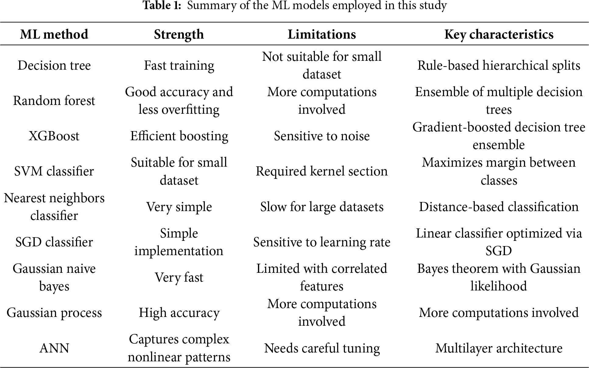
The summary of strengths, limitations and key characteristics of these models are given in Table 1.
3.1 Workflow for ML–Based Frameworks for Prediction of Crystal Structures
Fig. 1 presents the workflow employed in this study to predict the crystal structure of lithium manganese silicate cathodes using data sourced from the Materials Project. The dataset consisted of 211 DFT-computed entries containing the selected input features, while the output crystal structure was encoded as a binary label, with 0 representing monoclinic and 1 representing triclinic structures.
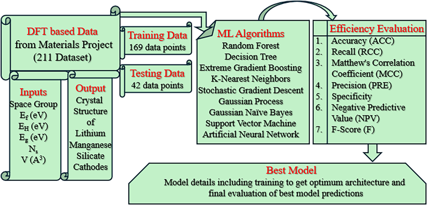
Figure 1: Workflow of the present study for predicting the crystal structure of lithium manganese silicate cathodes using Materials Project data
The data were divided into 169 training samples and 42 testing samples, and nine ML algorithms were applied to develop predictive models. This 80:20 division follows a widely accepted practice in machine-learning studies, providing a balanced compromise between model training and unbiased evaluation. The split was generated through random partitioning to avoid sampling bias and ensure that the model performance reflects true generalization to unseen data. Model performance was evaluated using multiple assessment metrics including accuracy (ACC), Matthew’s correlation coefficient (MCC), recall (RCC), precision (PRE), F-score (F), negative predictive value (NPV) using Eqs. (6)–(11). Based on overall prediction accuracy, the best-performing model was identified and subsequently subjected to detailed optimization and analysis of its architecture and predictive behavior.
Here, TP = true positive, TN = true negative, FP = false positve, FN = false negative.
3.2 Dataset Description and Preprocessing
The entire dataset was obtained from the Materials Project Database [9], which provides DFT computed properties of 211 cathode materials with Li-Si-(Mn)-O compositions. All DFT calculations and structural optimizations were performed using the VASP software within the Materials Project framework. The exchange–correlation potentials were treated using the generalized gradient approximation (GGA) or GGA + U, and the DFT energies for the Li-Si-(Mn)-O systems were generated through a high-throughput computational workflow. The initial DFT calculations containing positions of atoms and lattice parameters of crystals can be based on available data from inorganic crystal structure database [27].
The dataset includes the Ef, Eh, Eg, number of sites (Ns), density (ρ), the volume of the unit cell (V), and crystal structure of each electrode. The available dataset is divided into 80:20 as training and testing datasets. To avoid any bias in the training process, each method-based model is trained 100 times, and the models are stored. The data inputs are the chemical formula, space group, Ef (eV) Eh (eV), Eg (eV), Ns, ρ (g.cm−3) and V (A3). The output is the crystal structures of Li-Si-(Mn)-O cathode materials that are monoclinic (0) or triclinic (1). Fig. 2 presents the pair plot of the properties of Li-Si-(Mn)-O cathode materials in the dataset. The diagonal elements illustrate the distribution of individual features, while the off-diagonal plots show pairwise relationships between variables. The symmetry along the diagonal reflects similar distributions across parameters, and the axes appear mirrored due to the pairwise plotting arrangement.
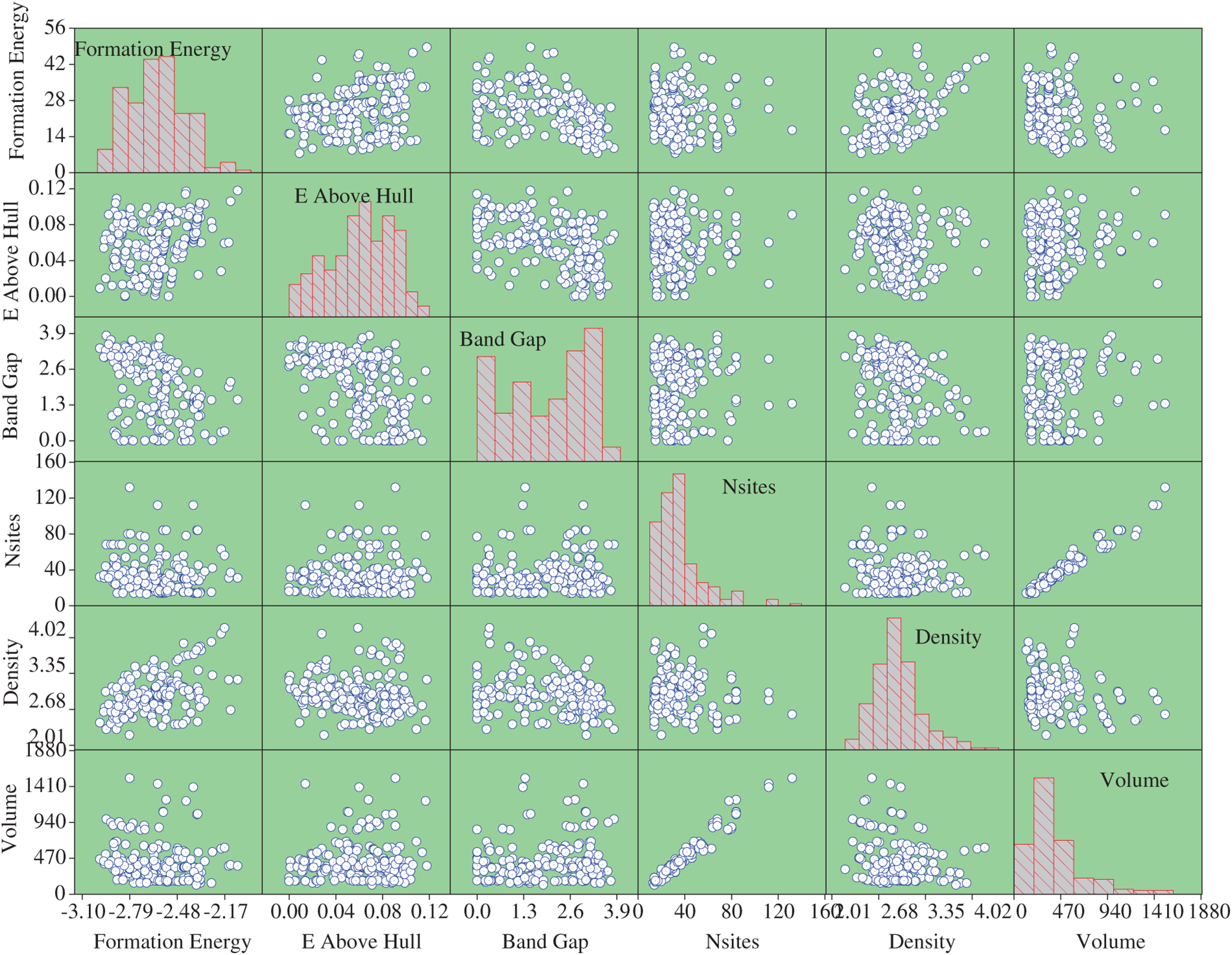
Figure 2: Pair plot of the properties of the Li-M-Si-O (M=Fe, Mn, and Co) cathode materials from Materials Project about the relative input parameter
No clear correlation is observed between the selected features and the resulting crystal system, highlighting that simple linear or direct relationships are insufficient to describe the underlying structure–property interactions. This lack of explicit trends underscores the necessity of employing advanced modelling techniques capable of capturing complex, nonlinear dependencies within the data. Therefore, ML-based modelling becomes essential for reliably predicting the crystal structures of lithium manganese silicate cathodes, where multiple compositional and structural factors interact in a non-trivial manner.
4.1 Prediction Performance of ML Models
A comparative assessment of each of the nine ML algorithms was conducted to evaluate their performance using various statistical indicators, including ACC, RCC, PRE, specificity, NPV, and F-score (Table 2). The results revealed substantial variability in the generalization capability of different models. The DT model exhibited good fitting during training (accuracy = 0.887) but demonstrated a sharp decline in testing accuracy (0.639), indicating overfitting. In contrast, the ensemble-based models, RF and XGBoost, showed superior performance, achieving nearly perfect training accuracies (1.000 and 0.993, respectively) and strong testing accuracies (0.803 and 0.721, respectively). Notably, RF outperformed all other models in terms of balanced accuracy, recall, and precision on the test set (accuracy = 0.803, recall = 0.786, precision = 0.917, F-score = 0.846), highlighting its robustness and effective handling of complex nonlinear relationships. The SVM classifier demonstrated moderate predictive ability (testing accuracy = 0.688), providing a stable but not outstanding performance. The Nearest Neighbors Classifier yielded lower testing accuracy (0.606), which may be attributed to its sensitivity to noise and local data variations.
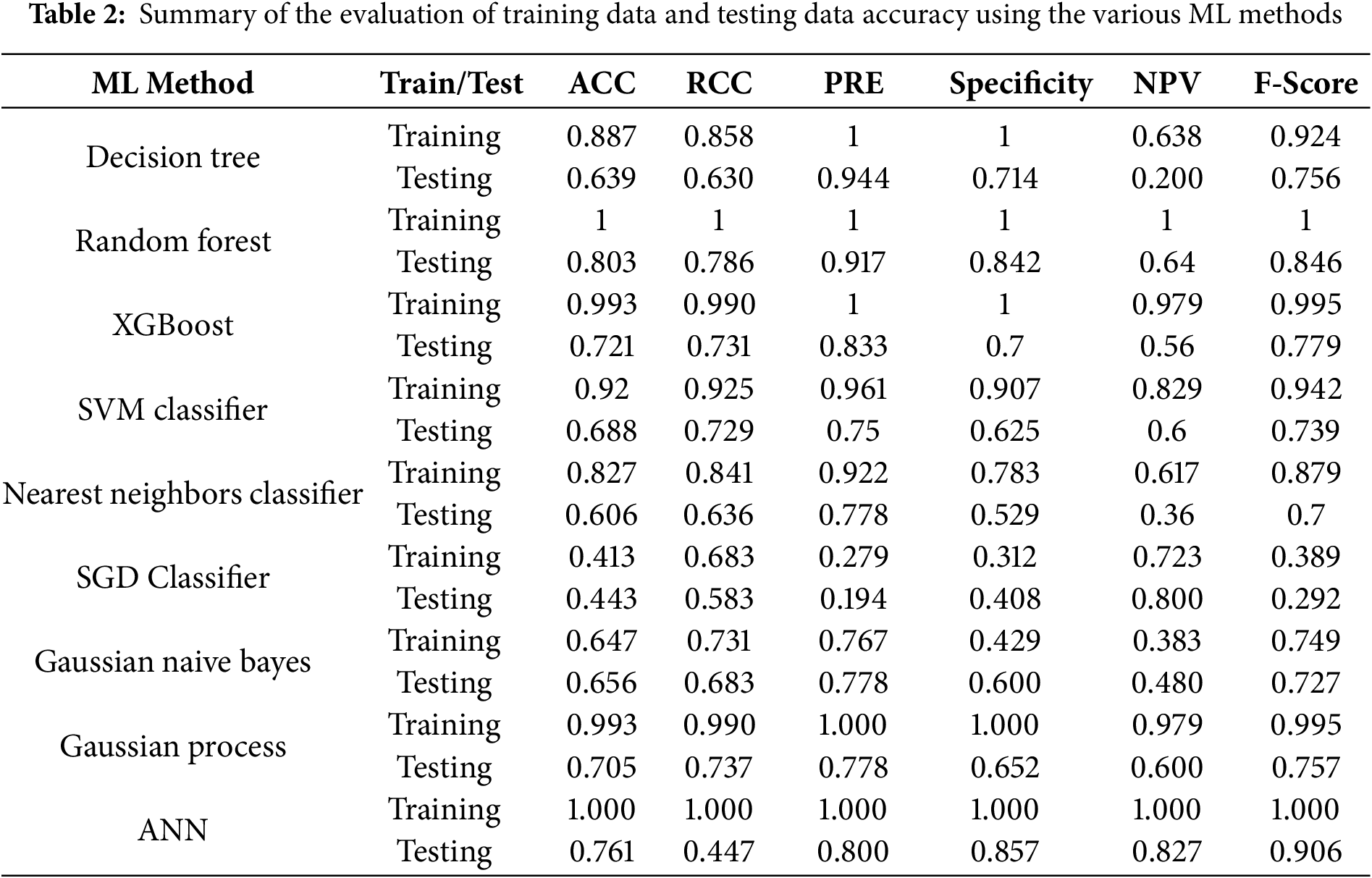
The SGD classifier exhibited the weakest performance across all metrics (testing accuracy = 0.443, F-score = 0.292), indicating poor convergence in nonlinear feature spaces. Among the probabilistic approaches, Gaussian NB and GP classifiers achieved comparable results, with the latter showing slightly higher predictive balance (testing accuracy = 0.705, F-score = 0.757). The ANN achieved perfect training accuracy (1.000) and demonstrated strong generalization on the testing dataset (accuracy = 0.761, F-score = 0.906). Although minor overfitting was observed, the ANN effectively captured intricate nonlinear dependencies, outperforming most conventional algorithms in terms of overall predictive reliability.
These findings suggest the ANN model achieved the highest prediction accuracy and demonstrated the strongest capability to learn the complex, nonlinear interdependencies among the input features. The remaining eight models were optimized using standard and widely accepted hyperparameter-tuning procedures (e.g., grid search, cross-validation, and built-in optimization routines), and their performance showed relatively low sensitivity to tuning variations. Therefore, an extensive architectural explanation was not required for them. In contrast, the ANN contains multiple architecture-dependent parameters such as the number of layers, neurons per layer, activation functions, learning rate, and momentum terms, and its performance was highly sensitive to these choices. To ensure transparency, fairness, and reproducibility, the detailed ANN architecture, optimization strategy, and training behavior will be provided in the coming sections.
4.2 Data Splitting for ANN Model
Fig. 3 shows the data classed for training and testing data in monoclinic and triclinic crystal structures. In the monoclinic crystal structure, 111 training data and 28 data out of 139 data were investigated, and the training data were not classified, with four of the testing data being unclassified. Also, 58 training data and 14 testing data out of the total 72 data were investigated in the triclinic crystal structure, and the triclinic crystal structure also showed unclassified data in the training data, and the testing data showed unclassified data in six testing data.
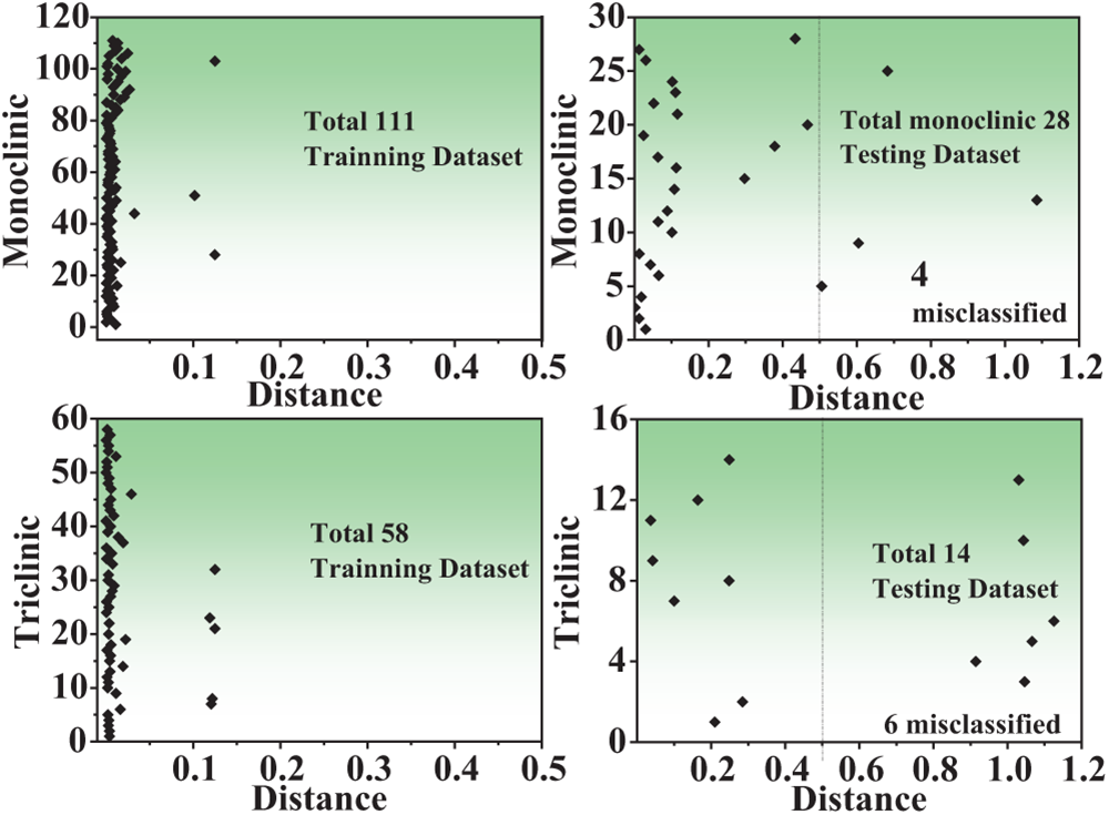
Figure 3: The misclassified training data and testing data in monoclinic and triclinic crystal systems
4.3 Optimum ANN Model Architecture
The ANN model was trained using the training dataset with systematic optimization of key hyperparameters. The core ANN algorithm was implemented in the C programming language for computational efficiency, while a user-friendly graphical user interface (GUI) was developed in Java to facilitate model execution, parameter adjustment, and visualization of results. The number of hidden layers were varied from 1 to 3, the number of neurons per layer from 1 to 30, the momentum coefficient from 0.1 to 1.0, the learning rate from 0.1 to 1.0, and the number of training iterations from 5000 to 70,000. The corresponding changes in model behavior under these settings are illustrated in Fig. 4. The optimized ANN architecture consists of three hidden layers with fourteen neurons in each layer (Fig. 4a). A momentum value of 0.3 (Fig. 4b), a learning rate of 0.6 (Fig. 4c), and 20,000 training iterations (Fig. 4d) yielded the best performance, achieving a prediction accuracy of 94.31%. Further refinement through iteration tuning demonstrated that the highest accuracy of 95.26% was reached at 20,000 iterations. These results clearly demonstrate the significant impact of hyperparameter selection on the ANN’s ability to accurately predict the crystal system of Li-Mn-Si-O materials.
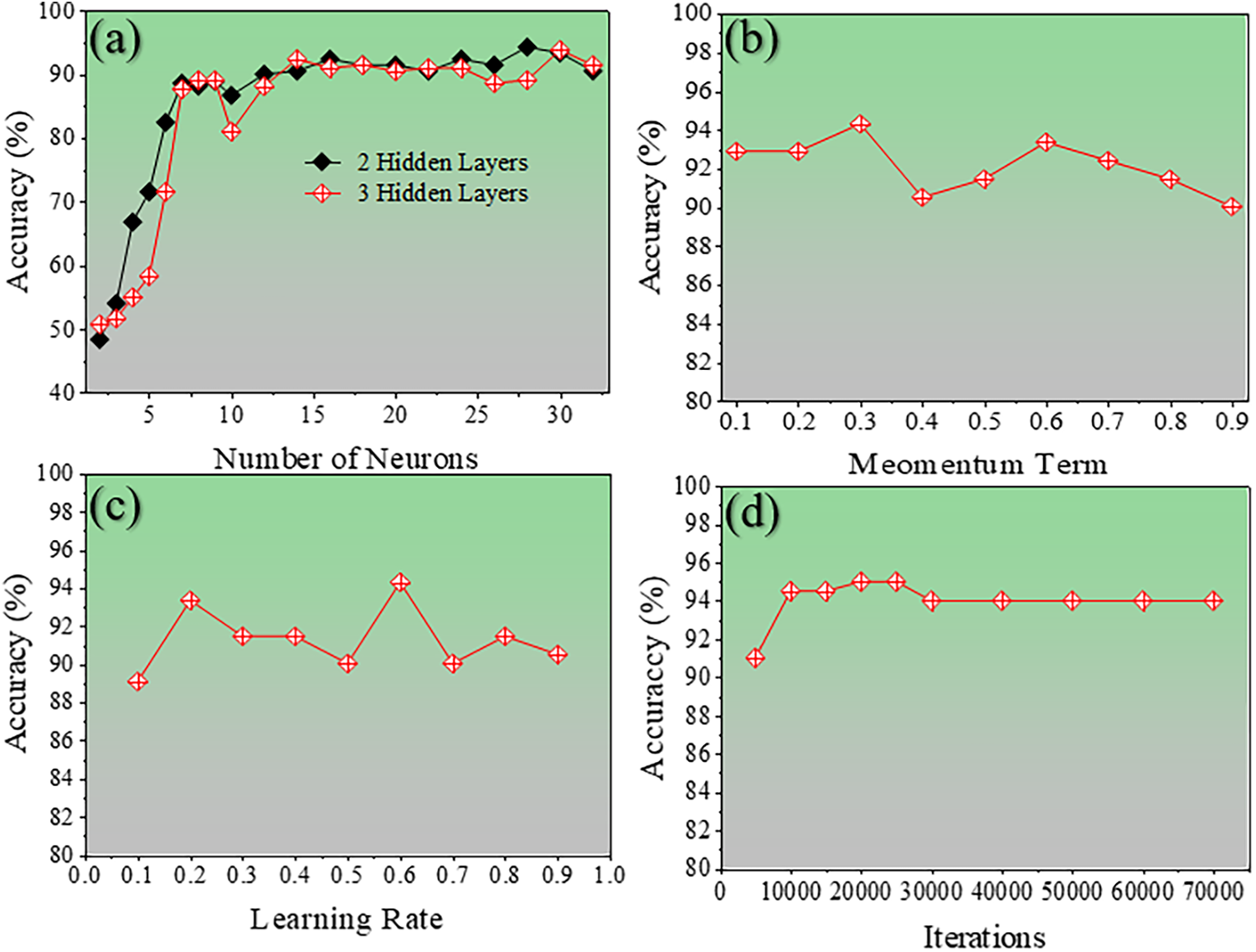
Figure 4: The line graphs show the accuracy of different hyperparameters for the ANN
All data, including the chemical formula, space group, experimental, and ANN predicted crystal structure, are presented in the Table 3. The four unclassified data are monoclinic crystal structures in the experimental crystal system and represent triclinic crystal structures in the ANN model. The six unclassified data represent the triclinic crystal structure in the experimental and the monoclinic crystal structure in the ANN model. The commonality of these is that the Space group is P1.

4.4 Evaluation of the Confusion Matrix
A confusion matrix between the ANN model and the DFT calculated data predicts all data in the dataset as either positive or negative. This classification produces four outcomes.
TP values are accurate positive predictions, FP values are incorrect positive predictions, TN shows accurate negative predictions, and FN represents incorrect negative predictions. The TP value represents the data number when the ANN model prediction and the DFT prediction are both monoclinic, and the TN values represent the data number when both the ANN model and the DFT prediction are Triclinic. Table 4 shows the evaluation of the confusion matrix. The total data sets are 211. The number of TP, FP, FN, and TN values show 135, 6, 4, and 66. To ensure the reliability of the classification results and to assess the performance of the ANN model, its predictions were compared with the corresponding DFT-calculated data. The model’s performance, evaluated using several statistical metrics, is presented in Fig. 5.
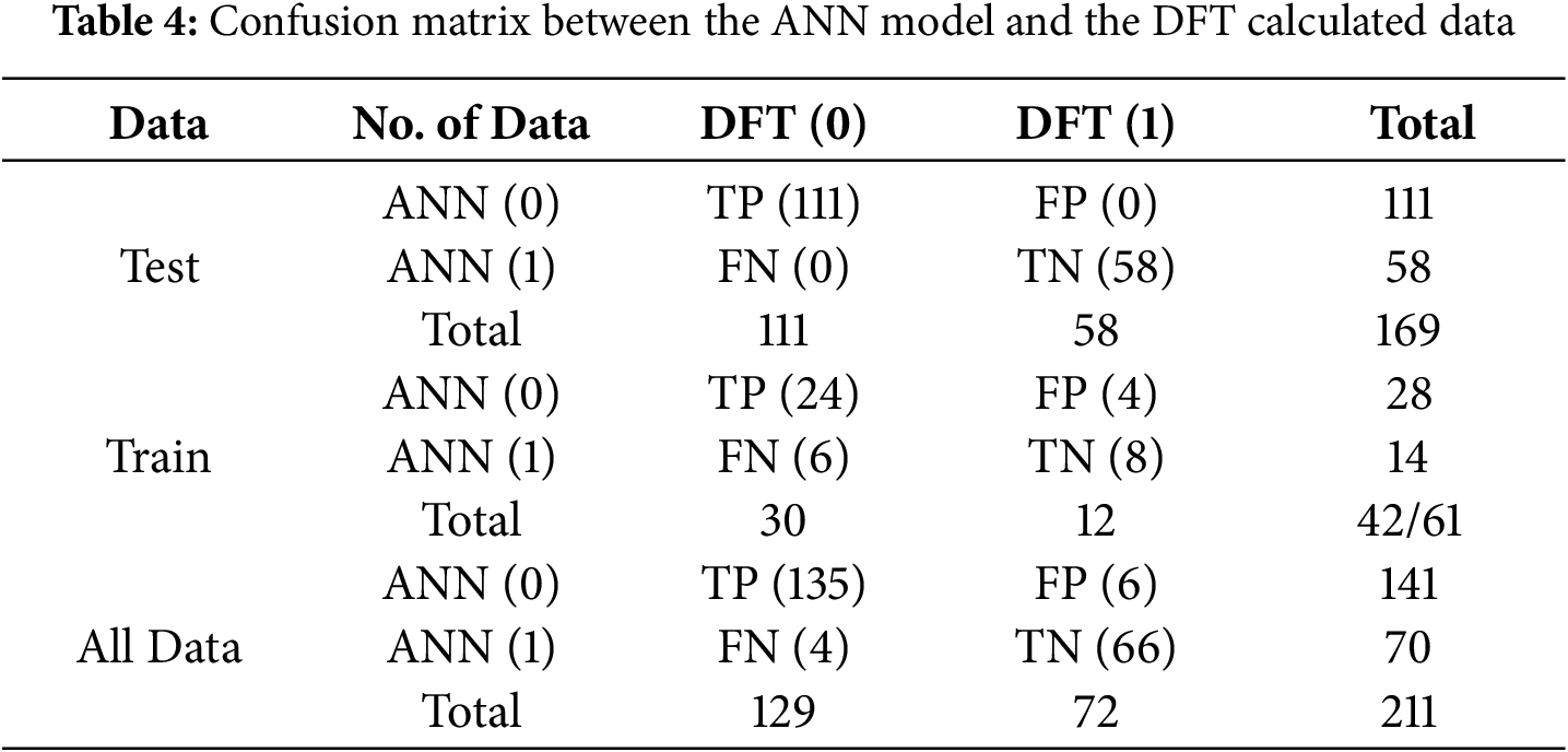
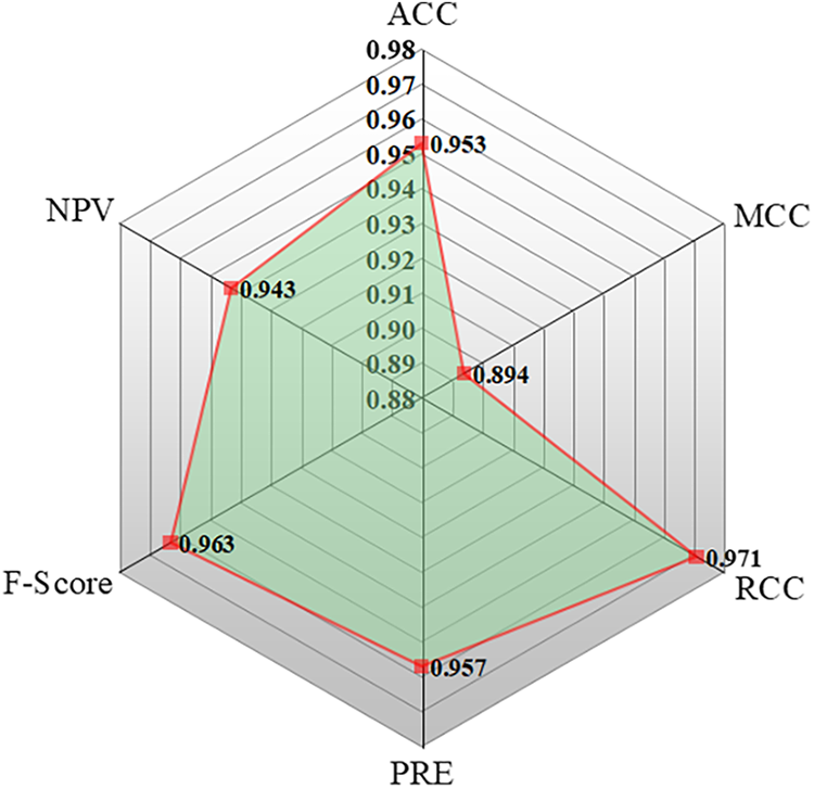
Figure 5: The spider plot showing the performance of ANN by different evaluation matrices
The ACC value of the optimized ANN model was found to be 0.953, indicating a high level of predictive reliability. The MCC, which evaluates the balance between under- and over-predictions—where MCC = 1 represents a perfect prediction and MCC = 0 corresponds to a random assignment—was 0.894, signifying strong consistency between predicted and actual classifications. The precision (PRE), representing the ratio of correctly predicted positive cases to all predicted positives, was 0.957. The F-score, defined as the harmonic mean of precision and recall (ideal value = 1), was 0.963, further confirming the model’s strong performance. The NPV, which measures the ratio of correctly predicted negatives to total predicted negatives, was 0.943, demonstrating that the model effectively distinguishes between the two crystal systems.
In this study, various machine learning (ML) algorithms were developed and compared for predicting the crystal system of lithium manganese silicate (Li-Mn-Si-O) cathode materials using density functional theory (DFT) data from the Materials Project database. The dataset contained 211 compositions with key features such as formation energy, energy above the hull, bandgap, number of atomic sites, density, and unit cell volume. These descriptors were used to classify the crystal system into monoclinic (0) and triclinic (1) phases.
The comparative analysis of multiple classification techniques—Decision Tree, Random Forest, XGBoost, Support Vector Machine, Nearest Neighbor Classifier, Stochastic Gradient Descent, Gaussian Naïve Bayes, Gaussian Process, and Artificial Neural Network (ANN)—revealed that the ANN model exhibited the highest predictive performance. The optimized ANN architecture (6–14-14-14-1) achieved an accuracy of 95.3%, a Matthews correlation coefficient (MCC) of 0.894, and an F-score of 0.963, indicating strong consistency between DFT-predicted and ANN-classified crystal systems. Random Forest and Gaussian Process models also showed high accuracies (0.803 and 0.705, respectively) and served as robust complementary approaches, particularly when data are limited or computational efficiency is required.
This study establishes a reliable ML-based framework for classifying lithium manganese silicate crystal structures, providing a solid foundation for future generative work. Although the present focus is classification, the developed model and insights will guide our next phase, where we aim to extend the approach toward predicting and generating new crystal structures.
The present study is limited by the size and scope of the available dataset, which restricts the application of advanced validation strategies and additional thermodynamic analyses such as convex-hull stability mapping. In addition, the current framework is focused on accurate crystal-structure classification rather than generative prediction of new structures, which represents an important next step for real-world materials discovery. Future work will focus on expanding the dataset, incorporating comprehensive phase-stability information, and extending the model toward generative and predictive capabilities, complemented by thermodynamic calculations and experimental validation to further strengthen the robustness and generality of the proposed approach.
Acknowledgement: Not applicable.
Funding Statement: This work was supported by the Learning & Academic Research Institution for Master’s, PhD students, and Postdocs LAMP Program of the National Research Foundation of Korea (NRF) grant funded by the Ministry of Education (No. RS-2023-00301974). This work was also supported by the Glocal University 30 Project fund of Gyeongsang National University in 2025.
Author Contributions: Conceptualization, Muhammad Ishtiaq and Nagireddy Gari Subba Reddy; methodology, Muhammad Ishtiaq and Yeon-Ju Lee; software, Annabathini Geetha Bhavani and Nagireddy Gari Subba Reddy; validation, Annabathini Geetha Bhavani and Yeon-Ju Lee; formal analysis, Yeon-Ju Lee and Muhammad Ishtiaq, investigation, Muhammad Ishtiaq and Nagireddy Gari Subba Reddy; resources, Sung-Gyu Kang; data curation, Annabathini Geetha Bhavani and Yeon-Ju Lee; writing—original draft preparation, Muhammad Ishtiaq; writing—review and editing, Sung-Gyu Kang and Nagireddy Gari Subba Reddy; supervision, Nagireddy Gari Subba Reddy and Sung-Gyu Kang. All authors reviewed the results and approved the final version of the manuscript.
Availability of Data and Materials: The authors confirm that the data supporting the findings of this study are available within the article.
Ethics Approval: Not applicable.
Conflicts of Interest: The authors declare no conflicts of interest to report regarding the present study.
Abbreviations
| ANN | Artificial Neural Network |
| DFT | Density Functional Theory |
| MCC | Matthews correlation coefficient |
| NPV | Negative Predictive Value |
| FP | False Positives |
| TP | True Positives |
| TN | True Negatives |
| FN | False Negatives |
References
1. Roy H, Roy BN, Hasanuzzaman M, Islam MS, Abdel-Khalik AS, Hamad MS, et al. Global advancements and current challenges of electric vehicle batteries and their prospects: a comprehensive review. Sustainability. 2022;14(24):16684. doi:10.3390/su142416684. [Google Scholar] [CrossRef]
2. Ali Ijaz Malik M, Kalam MA, Ikram A, Zeeshan S, Raza Zahidi SQ. Energy transition towards electric vehicle technology: recent advancements. Energy Rep. 2025;13:2958–96. doi:10.1016/j.egyr.2025.02.029. [Google Scholar] [CrossRef]
3. Wang N, Yin J, Li H, Wang T, Cui S, Yan W, et al. Recent advance in Mn-based Li-rich cathode materials: oxygen release mechanism and its solution strategies based on electronic structure perspective, spanning from commercial liquid batteries to all-solid-state batteries. Next Mater. 2025;6:100408. doi:10.1016/j.nxmate.2024.100408. [Google Scholar] [CrossRef]
4. Lee S, Jin W, Kim SH, Joo SH, Nam G, Oh P, et al. Oxygen vacancy diffusion and condensation in lithium-ion battery cathode materials. Angew Chem Int Ed. 2019;58(31):10478–85. doi:10.1002/anie.201904469. [Google Scholar] [PubMed] [CrossRef]
5. Arroyo-de Dompablo ME, Armand M, Tarascon JM, Amador U. On-demand design of polyoxianionic cathode materials based on electronegativity correlations: an exploration of the Li2MSiO4 system (M=Fe, Mn, Co, Ni). Electrochem Commun. 2006;8(8):1292–8. doi:10.1016/j.elecom.2006.06.003. [Google Scholar] [CrossRef]
6. Duncan H, Kondamreddy A, Mercier PHJ, Le Page Y, Abu-Lebdeh Y, Couillard M, et al. Novel Pn polymorph for Li2MnSiO4 and its electrochemical activity as a cathode material in Li-ion batteries. Chem Mater. 2011;23(24):5446–56. doi:10.1021/cm202793j. [Google Scholar] [CrossRef]
7. Luo Y, Gao X, Dong M, Zeng T, Chen Z, Yang M, et al. Exploring the structural properties of cathode and anode materials in Li-ion battery via neutron diffraction technique. Chin J Struct Chem. 2023;42(5):100032. doi:10.1016/j.cjsc.2023.100032. [Google Scholar] [CrossRef]
8. Nowakowski P, Bonifacio C, Ray M, Fischione P. The crystal orientation of Li metal anodes: a better understanding of lithium-ion solid-state batteries. Microsc Microanal. 2024;30:ozae044.878. doi:10.1093/mam/ozae044.878. [Google Scholar] [CrossRef]
9. Jain A, Ong SP, Hautier G, Chen W, Richards WD, Dacek S, et al. Commentary: the materials project: a materials genome approach to accelerating materials innovation. APL Mater. 2013;1:011002. doi:10.1063/1.4812323. [Google Scholar] [CrossRef]
10. Ren D, Wang C, Wei X, Zhang Y, Han S, Xu W. Harmonizing physical and deep learning modeling: a computationally efficient and interpretable approach for property prediction. Scr Mater. 2025;255:116350. doi:10.1016/j.scriptamat.2024.116350. [Google Scholar] [CrossRef]
11. Shandiz MA, Gauvin R. Application of machine learning methods for the prediction of crystal system of cathode materials in lithium-ion batteries. Comput Mater Sci. 2016;117:270–8. doi:10.1016/j.commatsci.2016.02.021. [Google Scholar] [CrossRef]
12. Wang G, Fearn T, Wang T, Choy KL. Machine-learning approach for predicting the discharging capacities of doped lithium nickel-cobalt–manganese cathode materials in Li-ion batteries. ACS Cent Sci. 2021;7(9):1551–60. doi:10.1021/acscentsci.1c00611. [Google Scholar] [PubMed] [CrossRef]
13. Ng MF, Zhao J, Yan Q, Conduit GJ, Seh ZW. Predicting the state of charge and health of batteries using data-driven machine learning. Nat Mach Intell. 2020;2(3):161–70. doi:10.1038/s42256-020-0156-7. [Google Scholar] [CrossRef]
14. Wang Y, Jiang B. Attention mechanism-based neural network for prediction of battery cycle life in the presence of missing data. Batteries. 2024;10(7):229. doi:10.3390/batteries10070229. [Google Scholar] [CrossRef]
15. Zhang Y, Feng X, Zhao M, Xiong R. In-situ battery life prognostics amid mixed operation conditions using physics-driven machine learning. J Power Sources. 2023;577:233246. doi:10.1016/j.jpowsour.2023.233246. [Google Scholar] [CrossRef]
16. Longo RC, Xiong K, Santosh KC, Cho K. Crystal structure and multicomponent effects in Tetrahedral Silicate Cathode Materials for Rechargeable Li-ion Batteries. Electrochim Acta. 2014;121:434–42. doi:10.1016/j.electacta.2013.12.104. [Google Scholar] [CrossRef]
17. Prosini PP. Crystal group prediction for lithiated manganese oxides using machine learning. Batteries. 2023;9(2):112. doi:10.3390/batteries9020112. [Google Scholar] [CrossRef]
18. Sun Z, Wang G, Li P, Wang H, Zhang M, Liang X. An improved random forest based on the classification accuracy and correlation measurement of decision trees. Expert Syst Appl. 2024;237:121549. doi:10.1016/j.eswa.2023.121549. [Google Scholar] [CrossRef]
19. Rokach L, Maimon O. Decision trees. In: Maimon O, Rokach L, editors. Data mining and knowledge discovery handbook. Boston, MA, USA: Springer; 2006. p. 165–92. doi:10.1007/0-387-25465-x_9. [Google Scholar] [CrossRef]
20. Chen T, Guestrin C. XGBoost: a scalable tree boosting system. In: Proceedings of the 22nd ACM Sigkdd International Conference on Knowledge Discovery and Data Mining; 2016 Aug 13–17; San Francisco, CA, USA. doi:10.1145/2939672.2939785. [Google Scholar] [CrossRef]
21. Halder RK, Uddin MN, Uddin MA, Aryal S, Khraisat A. Enhancing K-nearest neighbor algorithm: a comprehensive review and performance analysis of modifications. J Big Data. 2024;11(1):113. doi:10.1186/s40537-024-00973-y. [Google Scholar] [CrossRef]
22. Tian Y, Zhang Y, Zhang H. Recent advances in stochastic gradient descent in deep learning. Mathematics. 2023;11(3):682. doi:10.3390/math11030682. [Google Scholar] [CrossRef]
23. Deringer VL, Bartók AP, Bernstein N, Wilkins DM, Ceriotti M, Csányi G. Gaussian process regression for materials and molecules. Chem Rev. 2021;121(16):10073–141. doi:10.1021/acs.chemrev.1c00022. [Google Scholar] [PubMed] [CrossRef]
24. Peretz O, Koren M, Koren O. Naive Bayes classifier-An ensemble procedure for recall and precision enrichment. Eng Appl Artif Intell. 2024;136:108972. doi:10.1016/j.engappai.2024.108972. [Google Scholar] [CrossRef]
25. Cortes C, Vapnik V. Support-vector networks. Mach Learn. 1995;20(3):273–97. doi:10.1007/BF00994018. [Google Scholar] [CrossRef]
26. Wang SC. Artificial neural network. In: Interdisciplinary computing in Java programming. Boston, MA, USA: Springer; 2003. p. 81–100. doi:10.1007/978-1-4615-0377-4. [Google Scholar] [CrossRef]
27. Hinuma Y, Hayashi H, Kumagai Y, Tanaka I, Oba F. Comparison of approximations in density functional theory calculations: energetics and structure of binary oxides. Phys Rev B. 2017;96(9):094102. doi:10.1103/physrevb.96.094102. [Google Scholar] [CrossRef]
Cite This Article
 Copyright © 2026 The Author(s). Published by Tech Science Press.
This work is licensed under a Creative Commons Attribution 4.0 International License , which permits unrestricted use, distribution, and reproduction in any medium, provided the original work is properly cited.
 Downloads
 Citation Tools