Enhanced Scene Recognition via Multi-Model Transfer Learning with Limited Labeled Data

1  Introduction

The significance of scene recognition is pivotal in diverse computer vision applications, endowing machines with the capability to comprehensively understand and interpret their surrounding environments [1]. Traditional scene recognition methods have long depended on hand-crafted feature descriptors such as Scale-Invariant Feature Transform (SIFT) [2,3], Histogram of Oriented Gradients (HOG) [2,3], and Speeded-Up Robust Features (SURF) [2,3]. Although these techniques are effective for specific applications, they present several inherent drawbacks. They often fail to capture high-level semantic information and complex spatial relationships within a scene. They also require substantial domain expertise for their design and tuning. In addition, they show limited robustness to variations in viewpoint, lighting, and occlusion. These methods typically demand large labeled datasets for proper training [3], which makes them time-consuming and difficult to scale. Consequently, traditional approaches often struggle to generalize about unseen environments [3].

Deep learning has introduced a transformative shift in overcoming these limitations. Convolutional Neural Networks (CNNs) and transfer learning reduce the need for extensive labeled datasets by utilizing knowledge from models pre-trained on large-scale image repositories such as ImageNet. In this study, we employ two pre-trained architectures: DenseNet201 [4] and VGG-16 [5], which are selected for their complementary advantages. DenseNet201 uses dense connectivity to promote feature reuse, improve gradient flow, and support efficient parameter learning. This design enables the extraction of rich, hierarchical representations suitable for modeling complex scene semantics with limited training data. VGG-16, characterized by its uniform stacked convolutional layers, excels at capturing fine-grained spatial features. By fusing features from both models, the proposed approach benefits from deep representations with strong semantic and structural detail capabilities that are difficult to achieve with manual feature engineering. The pre-trained networks function as powerful feature extractors, capturing complex patterns and semantic cues that enhance the robustness and adaptability of the scene recognition system [6]. Recent research reflects increased interest in deep learning and transfer learning for scene recognition [7–9], demonstrating improved generalization and adaptability to new environments. Recent techniques [10–12] for remote sensing scene recognition have enhanced CNN to generate robust prediction. Besides, many literature surveys [13–15] have identified the role of deep learning as an effective approach for scene recognition. The authors of [16] have analyzed the characteristics of AID that is a standard dataset for testing deep learning models in remote sensing. Recent works [17–19] continue to improve scene recognition results by reinforcing the role of preprocessing, multi-model features, and foundational descriptors. However, many prior works still face challenges in achieving high accuracy while minimizing reliance on labeled data and computational resources.

In this paper, we introduce an inventive scene recognition approach that mitigates these challenges through multi-model transfer learning techniques. By employing a diverse set of pre-trained deep neural networks, rich representations learned from large-scale datasets can be fine-tuned to achieve superior performance, even with limited labeled data. Our contributions include the introduction of a novel scene recognition method based on transfer learning, demonstrating its efficacy in achieving high accuracy with constrained labeled data, improving the efficiency of scene recognition for real-time applications, and overcoming limitations of traditional approaches through the utilization of various pre-trained models. Our principal contributions encompass the following:

•   Proposing an innovative scene recognition method grounded in multi-model transfer learning techniques. Our approach overcomes the limitations of previous works by leveraging multi-model transfer learning. Unlike single-modal approaches, which may struggle with domain gaps and limited feature representation, our method integrates information from diverse modalities. This promotes flexibility in various situations and enriches the acquired representations.

•   We address the computational overhead associated with fine-tuning pre-trained models by introducing an efficient method tailored for scene recognition. Unlike previous methods that may rely solely on exhaustive fine-tuning or require large datasets, our approach optimizes model adaptation on limited labeled data. This minimizes annotation work and optimizes the use of computational resources.

•   Enhancing the efficiency of scene recognition, rendering it well-suited for real-time applications. This contrasts with previous approaches that may sacrifice runtime efficiency for improved accuracy or vice versa. Our technique, which strikes a compromise between efficiency and performance, is ideal for deployment in resource-constrained environments and time-sensitive applications.

•   Surpassing the constraints associated with traditional methodologies by harnessing the formidable capabilities of deep neural networks. By autonomously developing hierarchical representations from data, utilizing pre-trained models trained on large-scale datasets, and customizing model architecture and optimization techniques, we achieve superior performance, scalability, and adaptability to diverse environmental contexts.

2  Related Works

Previous research in scene recognition has predominantly focused on handcrafted features, such as SIFT, HOG, or SURF [20–22]. Although these methods have shown promising results, they often struggle to capture complex scene characteristics and generalize well to unseen scenes. Additionally, the reliance on large, labeled datasets for training poses a significant challenge. Finally, conventional methods relying on manual feature engineering struggle with capturing intricate details in scenes, leading to reduced adaptability to diverse environments. In this Section, we will outline our approach to evaluating recent papers on scene recognition utilizing pretrained models. We will discuss each method individually and conduct a comparative analysis with our proposed approach, highlighting the advantages our method offers over existing techniques.

Recent improvements in deep learning and transfer learning have revolutionized scene recognition [13–15]. By utilizing pre-trained deep neural networks, researchers have achieved remarkable results in various computer vision tasks. However, most existing methods still require a substantial amount of labeled data for fine-tuning, limiting their practicality in scenarios with limited labeled data. Both manual and deep learning methods encounter difficulties in generalizing effectively to novel scenes due to inherent limitations in their feature representations. Lima and Marfurt [7] conducted a comprehensive analysis of transfer learning implementations for scene categorization using different datasets and deep-learning models. The evaluation examines the influence of specialization in different CNN models on the transfer learning process through the division of the original models at different stages. The results emphasize the significant impact of hyperparameters on the ultimate performance of the models. Remarkably, utilizing transfer learning from models created on larger, more general natural image datasets outperforms direct training on smaller remote sensing datasets. However, the results highlight that transfer learning is a strong method for identifying remote sensing situations. This indicates that transfer learning has the potential to improve the accuracy and efficiency of classification in this field. Zhao et al. [8] proposed a technique to classify remote-sensing scenes by resolving differences in input features between the target and source datasets. Principal component analysis (PCA) is used to extract filters from source images. These filters are then applied to target images in order to build an adapted dataset. A preexisting CNN is used to this modified dataset to extract features. These features are then used for classification with a classifier, resulting in highly accurate remote-sensing scene classification. The researchers achieved a total accuracy of 78.21% by utilizing the 50-layer Residual Network (ResNet-50) model on the AID dataset. The authors observed that the ResNet model’s performance was negatively affected by overfitting, which was attributed to its 50 layers. This was because the pretrained ResNet utilized in the experiment was initially intended for the ImageNet dataset, leading to inferior performance. Our approach uses DenseNet, which incorporates dense connection to ensure that each layer is connected to every other layer in a feed-forward way. The utilization of dense connections in this design resulted in enhanced accuracy when compared to ResNet. This improvement can be attributed to the improved flow of gradients and the increased reuse of features, which eventually mitigated overfitting and enhanced the accuracy of classification. Li et al. [9] introduced a technique for categorizing high-resolution remote sensing photographs that employs transfer learning and a feature extraction network with several models. The method uses pretrained CNN models to extract properties from remote sensing images, which are subsequently combined into a one-dimensional feature vector. This framework for deep feature extraction improves the expression of features, helping to efficiently capture features in remote sensing images. Following the extraction of features, a dropout layer and a fully connected layer are implemented, subsequently leading to classification. Despite their use of multi-model pretrained models, achieving a commendable accuracy of 93%, which is less than our results, obtained using five pretrained models, our method stands out for its simplicity and efficiency, utilizing only two pretrained models. Qi et al. [10] introduced a scene classification approach that uses a deep Siamese convolutional network and rotation invariance regularization. The method employs a distinctive technique of data augmentation specifically designed for the Siamese model to enhance the acquisition of rotation invariance. The goal function of the model incorporates a rotation invariance regularization requirement, in addition to the typical cross-entropy cost function employed in traditional CNN models. They obtained a recognition accuracy of 94.9% using ResNet-50 with rotation invariance regularization (RIR) on AID database. Despite Qi et al. [10] achieving a recognition accuracy of 94.9%, our method achieved a slightly lower accuracy of 93.65%. However, our method’s superiority lies in its ability to learn richer representations from diverse modalities, transfer knowledge effectively, and generalize well to unseen environments. While Qi et al. [10] utilized a data augmentation strategy tailored for the Siamese model to facilitate learning of rotation invariance, our method does not rely on such augmentation techniques. This not only simplifies the implementation of our method but also reduces computational overhead and potential sources of error. Cao et al. [11] introduced a method named Self-Attention-based Deep Feature Fusion (SAFF) for remote sensing scene classification. SAFF utilizes a pre-trained CNN to extract many layers of feature maps from aerial data. Subsequently, it utilizes a nonparametric self-attention layer to improve the weight of spatial and channel information, hence highlighting the significance of intricate objects and making efficient use of rarely appearing features. The aggregated features are subsequently classified using a support vector machine (SVM), achieving an overall accuracy of 90.25%. He et al. [12] introduced the multilayer stacked covariance pooling (MSCP) method for remote sensing scene classification. MSCP combines multilayer feature maps obtained from pretrained CNN models. The framework involves extracting feature maps, stacking them, and computing a covariance matrix to capture complementary information from different layers. These covariance matrices serve as features for classification using an SVM. Finally, they are achieving an accuracy of 91.52% on the AID database.

Following the widespread success of CNNs, vision transformers have reshaped modern computer vision by introducing self-attention mechanisms capable of modeling long-range relationships. The survey in [23] has examined the role of essential transformers in remote sensing, while addressing their limitations in terms of computational complexity and their reliance on big datasets. The authors of [24] have focused on Vision Transformers (ViTs), comparing their performance with CNNs. Their study has demonstrated that ViTs combined with data augmentation techniques consistently outperform CNNs for satellite imagery. Dosovitskiy et al. [25] presented the ViT, which applies pure transformer architecture to sequences of image patches and achieves strong performance on large-scale image classification tasks. Liu et al. [26] later introduced the Swin Transformer, a hierarchical design with shifted windows that captures multi-scale information while remaining computationally efficient. In remote sensing, transformer-based models have demonstrated promising performance in scene classification tasks [26]. Recent surveys [18,19] also provide comprehensive and up-to-date reviews of advances in remote sensing scene classification, covering both CNN-based methods and transformer-driven architectures. It is important to note that the combination of features from multiple pre-trained CNNs, often referred to as model fusion or ensemble methods, is a well-established practice in remote sensing scene classification. Previous approaches have employed various fusion strategies including feature concatenation [12], covariance pooling [15], and attention-based fusion [14]. While these methods demonstrate the benefits of leveraging multiple feature sources, they often require substantial computational resources or complex training protocols. Furthermore, many existing fusion approaches are designed for scenarios with relatively abundant labeled data or do not explicitly address the challenges of limited training samples. Our work distinguishes itself by proposing streamlined yet effective multi-model architecture that is specifically optimized for data-efficient learning through a carefully designed fusion and fine-tuning protocol.

Our proposed method takes a significant leap forward by introducing a multi-model transfer learning approach. By leveraging a combination of pre-trained models such as DenseNet201 and VGG, we address the limitations inherent in both manual feature engineering and deep learning approaches as the following:

•   Multi-model transfer learning enables the extraction of high-level features from diverse modalities, allowing the model to efficiently learn intricate scene representations without the need for manual feature crafting.

•   The incorporation of pre-trained models facilitates the transfer of knowledge learned from extensive datasets, overcoming the dependency on large, labeled datasets and enhancing the robustness of our method in scenarios with limited annotated data.

•   The amalgamation of pre-trained models enhances the generalization capability of our method by leveraging learned representations from diverse scenes, mitigating the challenges associated with adapting to unseen environments.

3  Proposed Methodology

This Section discusses the dataset used in this study and the details of our methodology. Fig. 1 shows the general diagram of our multi-model transfer learning methodology.

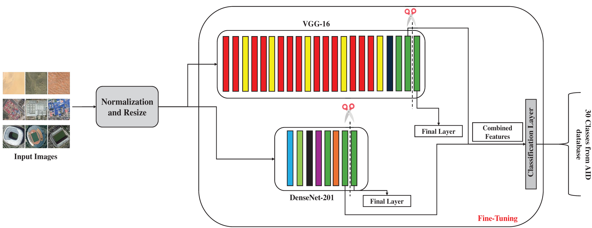
Figure 1: Block diagram of our methodology

3.1 Scene Classification Dataset

In this study we worked on AID dataset for scene classification [16]. The AID dataset has 30 distinct scene categories, with approximately 200 to 400 instances of size 600 × 600 in each category. AID is a new dataset of high-resolution aerial photos from Google Earth. The new dataset includes 30 aerial scene types as shown in Fig. 2.

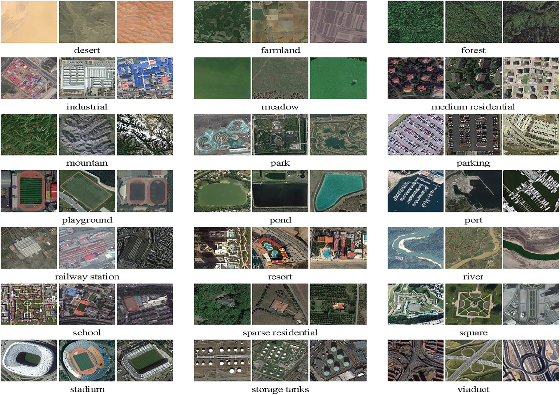
Figure 2: Representative examples of different classes

3.2 Multi-Model Transfer Learning Methodology

This section details our multi-model scene recognition methodology. It is important to clarify that in this work, the term ‘multi-model’ refers specifically to the fusion of features extracted from two different deep neural network architectures (DenseNet-201 and VGG-16) processing the same visual input, not from different data modalities such as text and images.

Our proposed scene recognition method follows the following steps:

Step 1: Preprocessing

•   Normalize and resize input images.

Step 2: Transfer Learning

•   Utilize a combination of pre-trained deep neural networks, such as DenseNet201 and VGG-16.

•   Remove the final classification layer from the base model and update some layers.

•   Freeze the weights of the base model to preserve the learned representations.

•   Add a new classification layer on top of the base model.

Step 3: Fine-tuning

•   Train the new classification layer using the labeled training data.

•   Fine-tune the entire network by gradually unfreezing the layers closer to the input.

•   Employ a suitable optimizer, such as Adam, and a learning rate schedule.

Step 4: Scene Recognition

•   Apply the trained model to classify scene images.

•   Assess the performance by utilizing criteria such as accuracy, precision, and recall.

In our recognition method, preprocessing serves as a critical initial step, essential for preparing input data to optimize deep neural network performance. Normalization and resizing play pivotal roles in standardizing input images and ensuring consistent dimensions [27]. This preprocessing not only streamlines subsequent operations but also aids in enhancing model generalization by minimizing variations in input data characteristics. In the first step, the input images undergo normalization and resizing. Normalization typically involves scaling pixel values to a standard range, such as [0, 1] or [−1, 1]. Resizing ensures that all images are consistent size, which is essential for feeding them into deep neural networks that often expect fixed input dimensions.

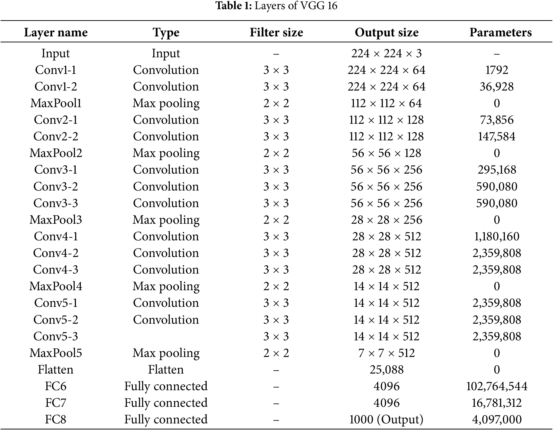
The method leverages pre-trained deep neural networks, specifically DenseNet201 and VGG (shown in Fig. 3 and Table 1). These networks are known for their strong feature extraction capabilities, having been trained on large datasets for image classification tasks. DenseNet-201 and VGG-16 are deep convolutional neural network architectures with 201 and 16 layers, respectively. DenseNet-201 introduces dense connections, while VGG-16 is known for its simplicity and effectiveness. The final model can be expressed mathematically as follows:

IntegratedModel(I)=Concatenate(DenseNet−201(I),VGG(I))(1)

here, I represents the image input. The dense block of DenseNet-201 can be defined as:

y=H([X0,X1,…,X(n−1)])(2)

where H denotes a series of operations, such as batch normalization, convolution, and activation, applied to the concatenated feature maps [X0, X1, … , X(n − 1)]. Each dense block contains multiple layers with shared weights. The specific equations for the operations within a dense block can be represented as:

Xi=Hi([X0,X1,…,X(n−1)])(3)

where Hi represents the composite function of batch normalization, convolution, and activation applied to the concatenated feature maps up to the (i − 1)th layer. A typical layer in VGG consists of a convolutional layer, batch normalization, and ReLU activation. Let x represent the input:

y=ReLU(BN(Conv2D(x)))(4)

where Conv2D denotes the convolutional layer, BN represents batch normalization, and ReLU is the activation function. For multi-model transfer learning, let I represents the image input. The integrated features can be obtained by concatenating the features from both DenseNet-201 and VGG:

IntegratedFeatures(I)=Concatenate(DenseNet−201Features(I),VGGFeatures(I))(5)

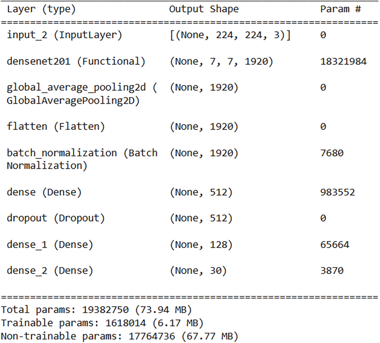
Figure 3: Layers of DenseNet-201

Eq. (1) provides a mathematical representation of the integrated model, highlighting the fusion of features extracted from DenseNet-201 and VGG-16. This fusion enables the model to leverage visual cues, capitalizing on multi-model learning’s strengths to enhance scene recognition performance. Additionally, Eqs. (2)–(4) shed light on the internal operations of DenseNet-201 and VGG-16, elucidating the processes within each network layer and the mechanisms driving feature extraction.

3.3 Feature Fusion Strategy

The foundation of our multi-model framework is the integration of features obtained from DenseNet-201 and VGG-16. Before fusion, the final classification layers of both pretrained networks are removed. We then extract the feature tensors produced by their last convolutional blocks. For an input image resized to 224 × 224 pixels, these tensors have the following shapes:

•   DenseNet-201: 7 × 7 × 1920

•   VGG-16: 7 × 7 × 512

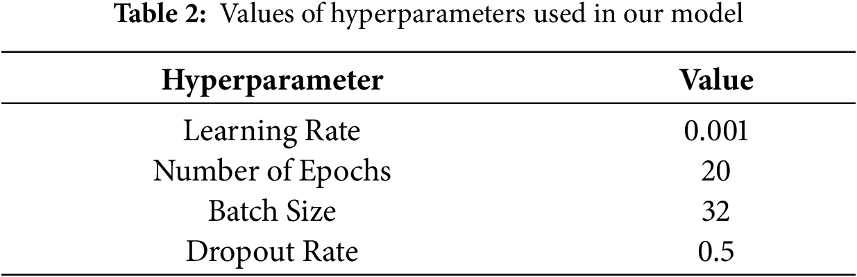
Each feature map is flattened into a one-dimensional vector. The DenseNet-201 features produce a vector of length 94,080 (7 × 7 × 1920), while the VGG-16 features result in a vector of length 25,088 (7 × 7 × 512). The two vectors are then concatenated channel-wise, forming a combined feature representation of 119,168 elements. Using this high-dimensional vector directly would introduce heavy computational cost and increase the risk of overfitting. To address this, we apply a dimensionality-reduction step through a fully connected projection layer. This layer uses ReLU activation and a dropout rate of 0.5, as shown in Table 2. It maps the concatenated vector into a more compact and discriminative feature space tuned into a hyperparameter. The resulting representation is then passed to the final classification layer. This strategy maintains strong representational capacity while improving efficiency and generalization.

The rationale behind selecting DenseNet-201 and VGG-16 as pre-trained deep neural networks can be further elaborated. The integration of dense connections in DenseNet-201 facilitates the construction of deeper network architectures while addressing the vanishing gradient problem, thereby contributing to improved feature representation. Conversely, VGG-16’s simplicity and effectiveness make it adept at capturing fine-grained details in images. Leveraging the complementary strengths of these architectures enables our method to extract diverse features from image inputs, enhancing the model’s discriminative power and robustness in scene recognition tasks.

3.4 Distinctive Aspects of Our Fusion Approach

Although feature fusion from multiple CNN backbones has been explored in prior studies, our method introduces several features that enhance its effectiveness, especially when labeled data are limited.

(1)   We intentionally pair DenseNet-201 with VGG-16 because their feature representations differ in meaningful ways. DenseNet-201 captures deep hierarchical information through dense connections, while VGG-16 provides strong sensitivity to local spatial patterns. Combining these complementary strengths leads to a richer and more informative scene representation than either model can achieve on its own.

(2)   Simple concatenation often produces very large feature vectors in our case, over 2000 dimensions, which can increase computational cost and reduce generalization. To address this, we apply a dimensionality reduction layer that projects the fused features into a more compact and discriminative space. This step lowers the computational burden and helps reduce issues associated with high-dimensional feature spaces.

(3)   Training follows a staged fine-tuning protocol. We initially updated only the newly added classification layers. We then gradually unfreeze deeper layers while maintaining strong regularization in the fusion layer (dropout of 0.5). This controlled adaptation allows the model to learn domain-specific patterns without losing valuable pre-trained knowledge—an essential consideration when working with small datasets.

(4)   Overfitting is a major challenge when combining high-capacity backbones. To counter this, we employ several regularization techniques: dropout in the fusion layer, L2 weight penalties, extensive data augmentation, and early stopping. Together, these methods stabilize training and promote strong generalization.

These design components set our method apart from standard multi-model fusion techniques. They also enable the model to perform effectively under limited supervision, addressing a common practical challenge in remote sensing applications.

Following this tailored fusion strategy, we proceed with adapting the pre-trained models for our specific scene recognition task. The final classification layers of the pre-trained backbones are removed, and selected layers such as fully connected layers are updated to align the models with the requirements of our scene recognition task. To preserve the rich representations learned during pre-training, the weights of the base networks are initially frozen, and a new classification head is added on top of the modified architecture. Because the multi-model has a high capacity and is trained in a limited-data setting, several regularization strategies are applied to reduce overfitting. A dropout layer with a rate of 0.5 is placed after the dimensionality reduction layer that follows feature concatenation. Real-time data augmentation, including random horizontal and vertical flips and rotations of up to 20 degrees, increases the diversity of the training samples. L2 weight regularization is applied to the fully connected layers to discourage overly large weights, and early stopping is used by monitoring the validation loss, halting training if no improvement occurs for 10 epochs and restoring the best-performing weights. A progressive fine-tuning protocol is also employed: only the newly added layers are trained during the first 5 epochs, after which layers in the pre-trained backbones are gradually unfrozen from top to bottom to ensure stable adaptation without catastrophic forgetting. Optimization is performed using the Adam optimizer with an initial learning rate of 0.001, supported by a learning-rate scheduling mechanism that reduces the learning rate by a factor of 0.1 when the validation loss plateaus. Together, these regularization methods and the carefully staged fine-tuning process enable the model to generalize effectively even with limited labeled data. The model is optimized using the Categorical

Cross-Entropy loss function, which is standard for multi-class classification tasks. The loss for a batch of N samples is computed as:

ℒ=−1N∑i=1N∑c=1Cyi,clog⁡(y^i,c)(6)

where C is the total number of scene classes (30 for the AID dataset), yi, c is the binary indicator (0 or 1) if class c is the correct classification for sample i, and y^i,c is the predicted probability (softmax output) for sample i belonging to class c.

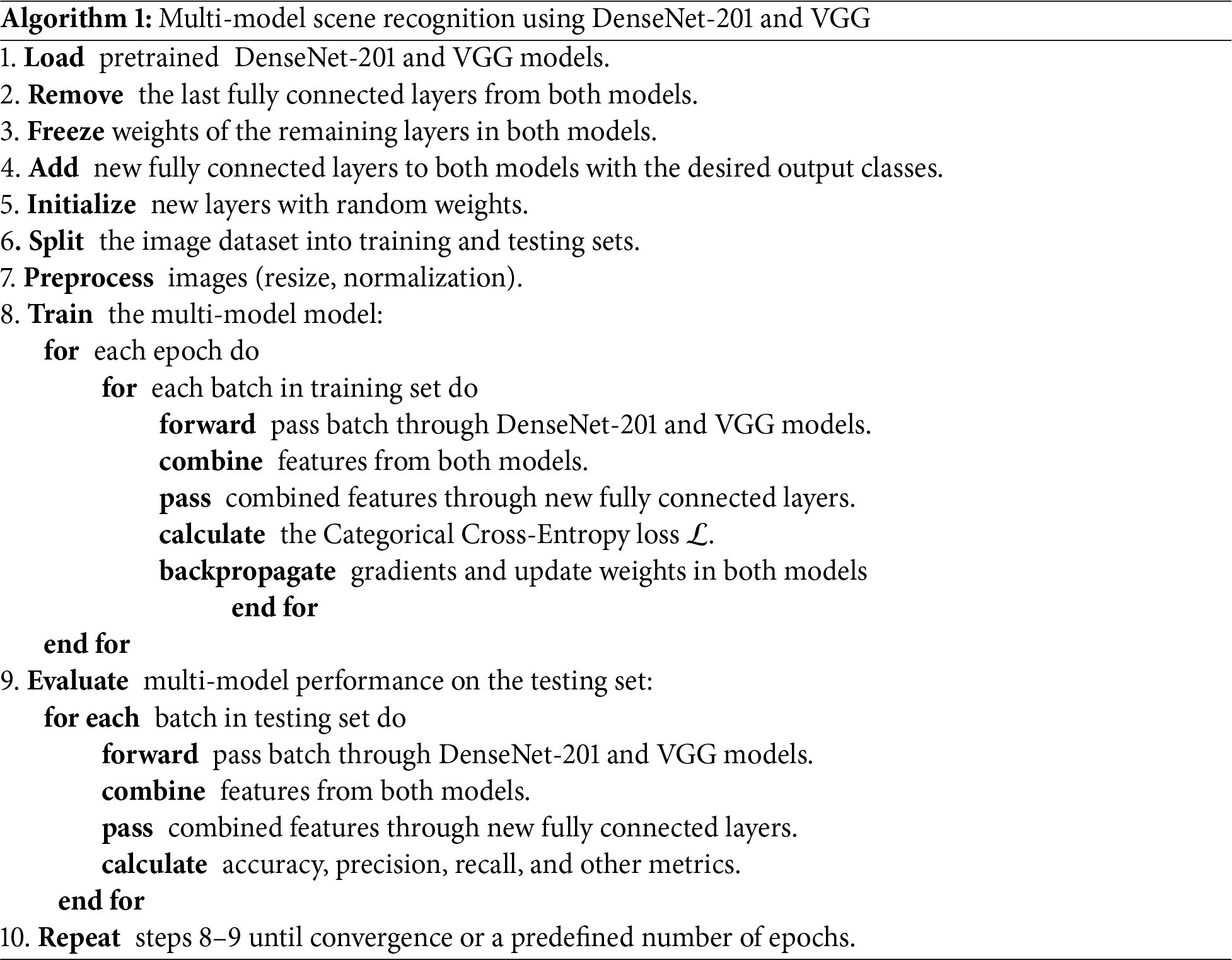
Once the model is trained, it is applied to classify scene images. The evaluation of the performance is conducted by employing several criteria, including accuracy, precision, and recall. These metrics offer valuable information about the model’s ability to generalize new data and its effectiveness in distinguishing between various scene types. We set the hyperparameters as shown in Table 2. The algorithm for the steps of our model is shown in Algorithm 1.

3.5 Performance Metrics

Evaluating the effectiveness and robustness of our model requires comprehensive analysis using appropriate performance metrics. In this section, we detail the metrics employed to assess the model’s classification accuracy and generalization capabilities across diverse scene categories.

(1)   Accuracy: The metric quantifies the ratio of accurately identified photos to the overall number of images in the evaluation dataset. A high accuracy score indicates that the model effectively distinguishes between different scene categories, demonstrating its capability to recognize scenes accurately. Can be computed as:

Accuracy=NumberofCorrectlyClassifiedSamplesTotalNumberofSamples×100\% (7)

(2)   Precision: It provides insights into the model’s ability to avoid misclassifying images from other categories as belonging to the target scene category. High precision indicates a low rate of false positives, signifying the model’s precision in identifying the target scenes. Can be computed as:

Precision=TPTP+FP(8)

where TP is the number of true positive predictions and FP is the number of false positive predictions.

(3)   Recall (Sensitivity): It indicates the model’s ability to capture all instances of the target scene category, without missing any. High recall values suggest that the model effectively recognizes most instances of the target scenes, demonstrating its sensitivity to scene characteristics. Can be computed as:

Recall=TPTP+FN(9)

where FN is the number of false negative predictions.

(4)   F1-Score: It functions as a complete measure for assessing the overall classification performance of the model, taking into account both precision and recall simultaneously. A high F1 score signifies an equilibrium between precision and recall, demonstrating the model’s resilience in scene recognition tests. Can be computed as:

F1−Score=2×Precision×RecallPrecision+Recall(10)

(5)   Confusion Matrix: It tabulates the actual and predicted labels for each scene category, enabling a thorough analysis of classification errors and misclassifications. By visualizing the confusion matrix, we can identify patterns of misclassification and areas for improvement in the model’s performance.

4  Results and Discussion

In this section, we present the results of our scene recognition model evaluation and discuss the implications of these findings. Utilizing the AID dataset [26], which comprises 30 distinct scene categories captured from high-resolution aerial photographs sourced from Google Earth, we assessed the performance of our model. The performance assessment involved a combination of quantitative metrics and qualitative analysis, shedding light on its accuracy, generalization capabilities, and potential areas for enhancement. The experiments were carried out using the TensorFlow and Keras libraries. The model’s performance is evaluated utilizing a machine setup comprising an Intel Core i5-10200H CPU @2.40 GHz (8 CPUs) with 24 GB RAM and an NVIDIA GeForce GTX 1650 GPU with 16 GB memory. Computational tasks were performed on cloud-based platforms, specifically Kaggle and Google Colab, utilizing their computational capacity and specialized deep learning frameworks such as TensorFlow and Keras. The model’s classification performance across several scene categories is quantified by calculating standard performance metrics including accuracy, precision, recall, and F1 score. Additionally, a confusion matrix is generated to visually represent the distribution of classification errors and misclassifications across different scene categories.

4.1 Qualitative Analysis

In conjunction with quantitative metrics, qualitative analysis is performed to assess the model’s ability to accurately recognize diverse scene categories. Fig. 4 shows sample images from the evaluation dataset that are visually inspected to verify the correctness of the model’s predictions and identify any potential misclassifications or ambiguities.

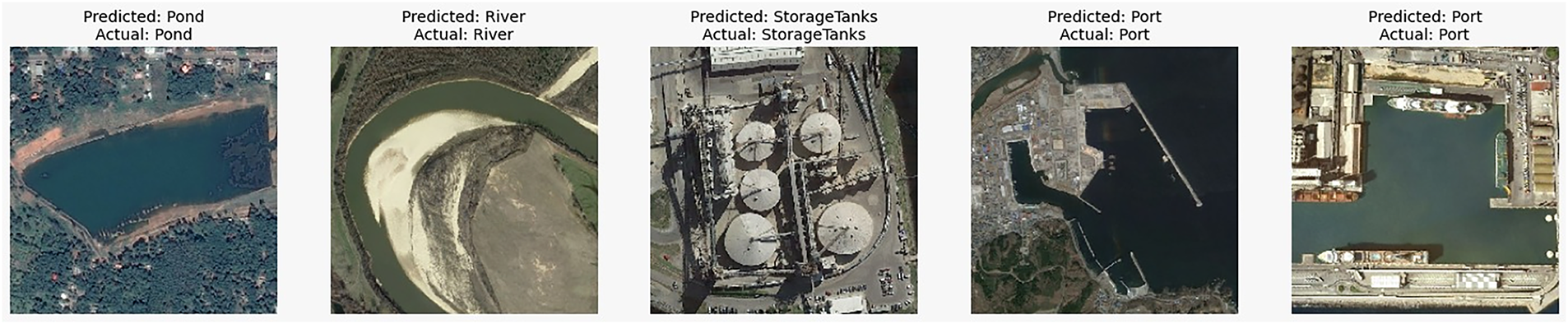
Figure 4: Visualize of the correctness of the model’s predictions

Moreover, the model’s performance is scrutinized under real-world conditions, accounting for factors such as lighting variations, occlusions, and scene composition differences. This qualitative assessment provides a comprehensive understanding of the model’s performance across various environmental contexts, as well as its robustness in practical applications. Fig. 5 shows plots of the training and validation accuracy and loss curves. The training accuracy curve in the Figure illustrates the improvement of the model’s performance on the training dataset over epochs. In the presented scenario, the training curve initiates at 75% accuracy in the first epoch and steadily ascends, reaching 95% accuracy by epoch 7. Subsequently, it experiences a slight increase, ultimately achieving a perfect accuracy of 100% by the final epoch. Conversely, the validation accuracy curve illustrates the model’s performance on unseen validation data throughout training. Beginning at 86% accuracy in the initial epoch, it exhibits a modest improvement, culminating in a validation accuracy of 93.6% by the final epoch. The loss curves depict the evolution of the model’s loss function, which quantifies the disparity between predicted and actual values. In the training loss curve, the loss begins at 0.8 in the first epoch and steadily diminishes, reaching 0.1 by epoch 7. Ultimately, it converges to 0 loss by the final epoch, indicating that the model fits the training data perfectly. Conversely, the validation loss curve commences at 0.35 loss in the first epoch. It experienced a slight decrease, reaching 0.3 loss by epoch 10, before witnessing a minor increase to 0.35 loss by the final epoch.

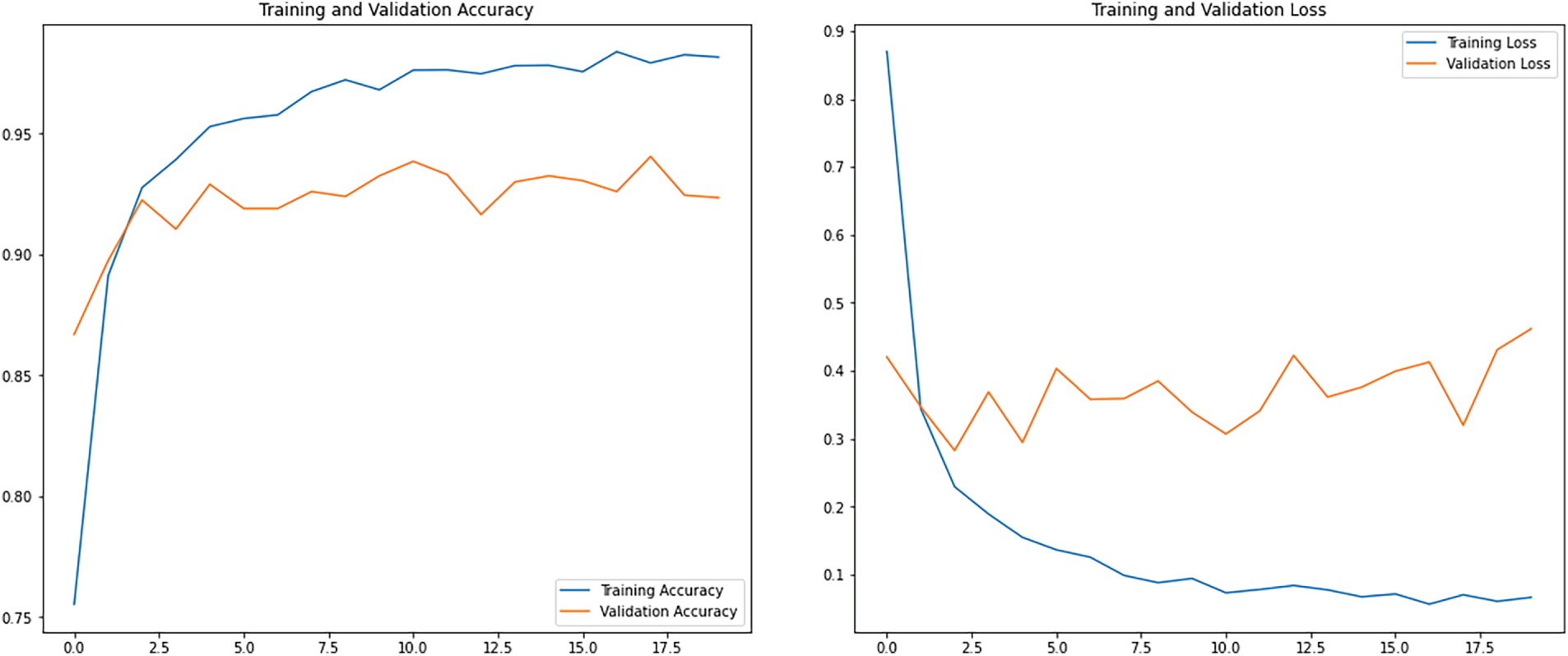
Figure 5: Training and validation accuracy and loss curves

The confusion matrix of the proposed method using the test images from AID dataset is presented in Fig. 6. The matrix contains information on the classifications made by the model for each of the 30 classes. Upon analyzing the confusion matrix, several key observations emerge regarding the model’s classification performance across the 30 classes of the AID dataset. Notably, the model demonstrates high accuracy in certain classes, correctly identifying all instances of class Baseballfield, for example. However, it exhibits varying degrees of misclassification across other classes. For instance, while it accurately identifies the majority of class Airport images, it misclassifies a few as classes Center, Industrial, SparseResidential, and Meadow. Similarly, class BareLand is mostly correctly identified, yet there are occasional misclassifications as class StorageTanks. Moreover, some classes, such as class Center, show a higher degree of misclassification with multiple instances of confusion with classes Chur, Commercial, SparseResidential, Playground, Meadow, and MediumResidential.

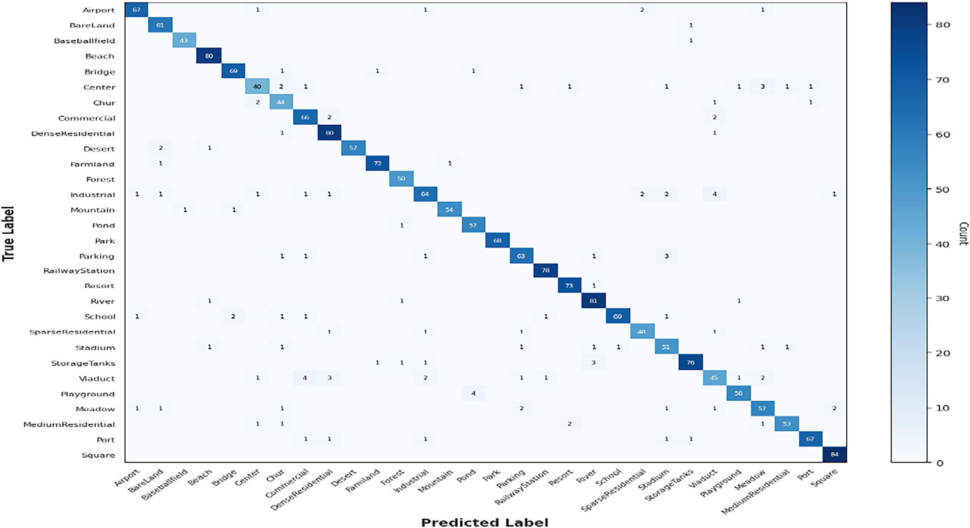
Figure 6: Confusion matrix for the test set from AID dataset

Table 3 presents a concise overview of the overall effectiveness of the proposed approach. From the Table, the precision value of 0.9367 signifies that approximately 93.67% of the instances predicted as positive by the model were indeed true positives. A recall value of 0.9365 indicates that approximately 93.65% of the actual positive instances were successfully captured by the model. The F1-score value of 0.9360 suggests a high overall performance of the model. Additionally, validation loss and validation accuracy are crucial metrics for assessing the overall performance of a model during the validation phase. Validation loss represents the error between the true labels and the model’s predictions on the validation dataset. A lower validation loss value of 0.3575 indicates better alignment between predicted and true values, reflecting improved model performance. Validation accuracy is the fraction of correctly categorized cases among all occurrences in the validation dataset. A validation accuracy of 0.9365 implies that approximately 93.65% of the validation dataset was correctly classified by the model. Fig. 7 displays a complete summary of the model’s performance for each specific class in the classification report.

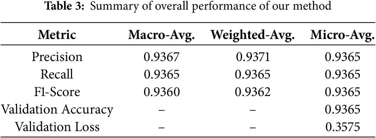
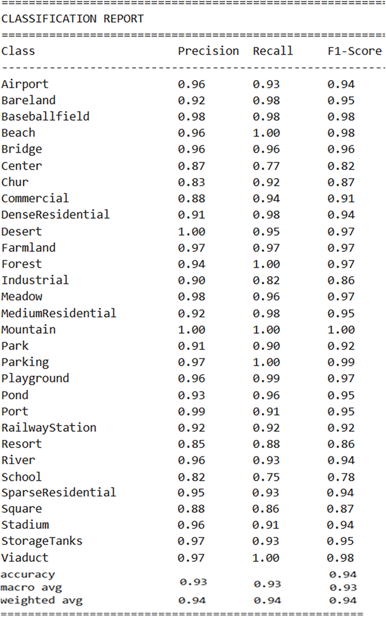
Figure 7: Classification report of our method for each class

4.2 Discussion

In this section, we will discuss the results of the proposed method based on the performance metrics used. We will discuss the efficiency of our method in accurately classifying instances across diverse classes within the dataset, highlighting strengths and areas for improvement. Furthermore, we will compare our method with recent papers in the field to contextualize our findings and assess state-of-the-art performance in similar classification tasks.

The findings of our methodology for remote sensing scene categorization give a detailed evaluation of the model’s performance, considering various metrics and comparisons with existing methods discussed throughout this conversation. Our method, leveraging a multi-model transfer learning approach with pre-trained models such as DenseNet201 and VGG, demonstrates promising results in scene classification accuracy. With a validation accuracy of 93.65% and a precision, recall, and F1-score averaging at 0.936, our method showcases robust performance across diverse scene categories.

From Fig. 5, the divergence between training and validation accuracies is an essential aspect to consider. Initially, the training accuracy surpasses the validation accuracy, indicating that the model may be overfitting the training data. However, as training progresses, the validation accuracy also improves, albeit at a slower pace, suggesting that the model generalizes well to unseen data. In addition, the convergence of the training loss to 0 signifies that the model effectively minimizes its error on the training data. Furthermore, the confusion matrix analysis provides valuable insights into the model’s classification behavior across different classes. While some classes exhibit high accuracy with minimal misclassifications, others may require further refinement to improve classification accuracy. Nonetheless, the overall balanced performance across classes underscores the efficiency of our proposed method in accurately identifying diverse scenes.

In the classification report in Fig. 7, precision values ranging from 0.83 to 1.00 across different classes highlight the model’s varied performance in accurately identifying instances within each class. In addition, the recall values reported in the classification report, ranging from 0.75 to 1.00, reflect the model’s capacity to identify true positive instances across diverse classes with varying degrees of success. The F1-scores reported in the classification report, ranging from 0.78 to 1.00, demonstrate the model’s robust performance across different classes, striking a balance between precision and recall.

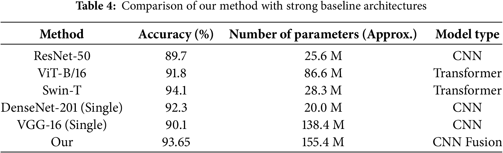
To better position the performance of our dual-stream model, we compared it with several well-established baseline architectures. All models were trained and evaluated under identical conditions, including the same data split, preprocessing steps, and hyperparameter tuning strategy. The single-model baselines included ResNet-50 [28], Vision Transformer Base (ViT-B/16) [29], and Swin Transformer Tiny (Swin-T) [30]. These models are widely recognized for their strong performance in visual recognition tasks, including remote-sensing applications. The results are presented in Table 4. They demonstrate that our proposed dual-stream model achieves a competitive balance between accuracy and model complexity. While the Swin-T transformer achieves the highest accuracy at 94.1% with a moderate parameter count of 28.3 M, our model, which strategically fuses two complementary CNNs, attains a strong accuracy of 93.65% with a higher parameter count (approximately 155.0 M). This parameter overhead is expected, as our approach incorporates the full convolutional bases of both DenseNet-201 and VGG-16, along with additional fusion and classification layers. Notably, our model outperforms the single-model baselines of ResNet-50, ViT-B/16, and the individual DenseNet-201 and VGG-16 models, confirming the advantage of feature fusion. This comparison highlights that our approach represents an effective and practical solution for scene recognition, particularly in scenarios where leveraging complementary architectural strengths is prioritized and computational resources permit the use of dual-stream architecture. The Swin-T attains a strong classification performance of 94.1% while employing a markedly smaller number of parameters (approximately 28.3 M) than the proposed dual-stream architecture (approximately 155.4 M), underscoring the relevance of parameter efficiency in model design. Nevertheless, the proposed multi-model fusion framework offers notable advantages in several practical contexts. From a computational perspective, although the overall parameter count is higher, the inference efficiency of the proposed model remains favorable. The feature extraction stages of DenseNet-201 and VGG-16 operate independently and can be executed in parallel during a forward pass. As a result, on the evaluation platform equipped with an NVIDIA GeForce GTX 1650, the proposed model achieved an average inference time of 15.2 ms per image, compared with 18.7 ms for Swin-T. This difference can be attributed to the relatively higher computational complexity of self-attention mechanisms in transformer-based architectures. In addition, the proposed approach is particularly well suited to scenarios with limited training data, where effective exploitation of pre-trained representations is essential. The staged fine-tuning strategy adopted for the CNN-based fusion model provides greater training stability and reduces susceptibility to overfitting on small datasets, in contrast to transformer models, which typically require larger volumes of data to fully realize their representational capacity. Consequently, the proposed method is especially advantageous for resource-constrained deployment settings that prioritize fast inference, as well as for application domains characterized by scarce labeled data but abundant, reliable pre-trained CNN features that can be efficiently integrated through feature-level fusion.

As shown in the accuracy and loss curves (Fig. 5), the training accuracy reaches 100%, whereas the validation accuracy stabilizes at 93.6%. This pattern indicates a moderate level of overfitting, which is expected when two high-capacity pre-trained models are combined and trained on a relatively small dataset. Nevertheless, the regularization strategies outlined in Section 3 especially dropout, data augmentation, and early stopping helped contain this overfitting. Their impact is reflected in the stable and consistently high validation accuracy. Although the model fits the training data almost perfectly, it still preserves strong generalization performance, which is the key requirement for real-world deployment.

A comparative analysis of our proposed method with recent methodologies outlined in Table 5.

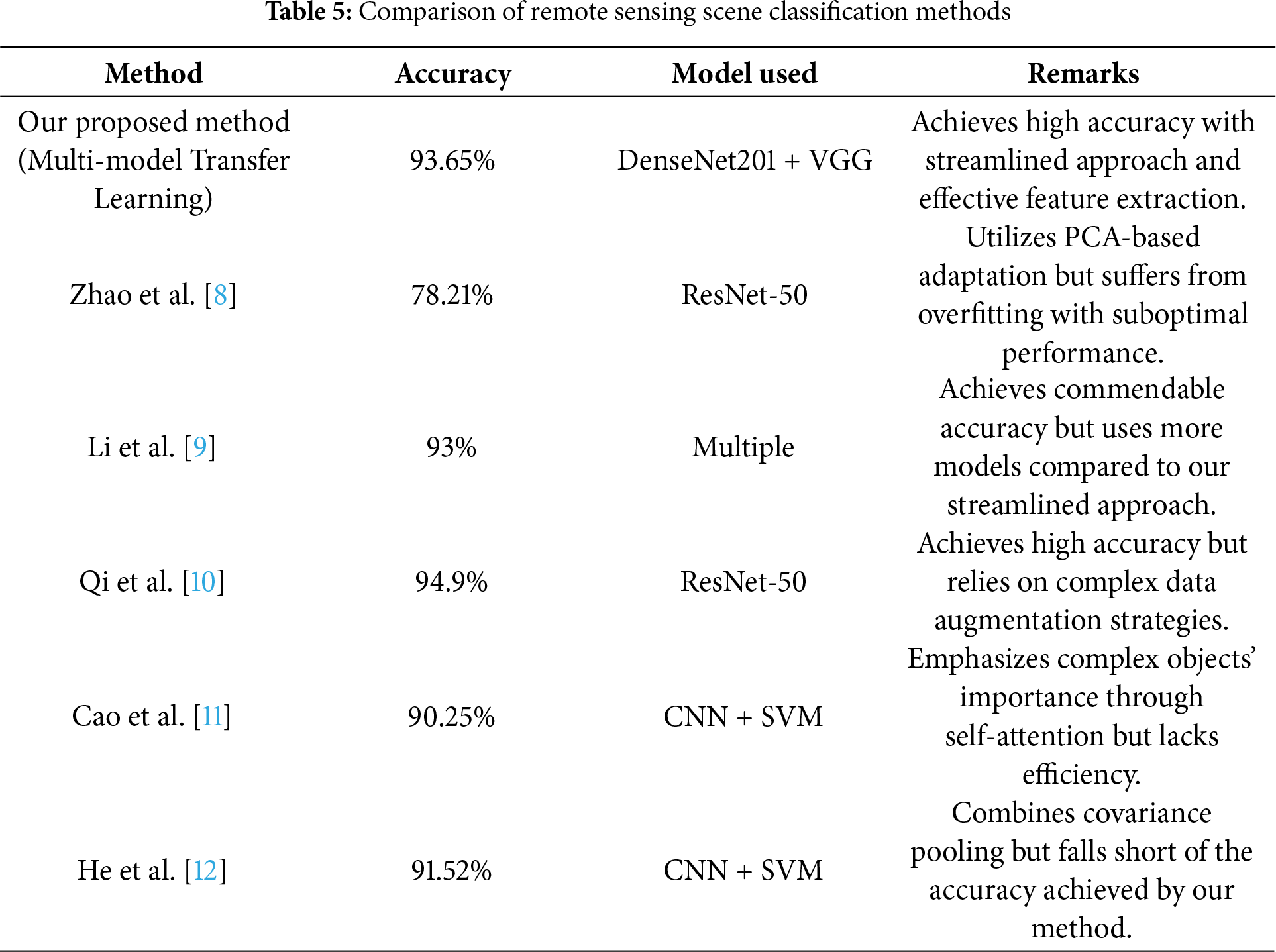
From the previous Table, our proposed method stands out for its high accuracy of 93.65%, achieved through the streamlined approach of leveraging DenseNet201 and VGG models for multi-model transfer learning. This approach ensures effective feature extraction while maintaining simplicity and efficiency. In comparison, Zhao et al. [8] achieved a lower accuracy of 78.21% with ResNet-50 due to overfitting, highlighting the importance of model architecture in remote sensing scene classification. Li et al. [9] achieved a commendable accuracy of 93% but utilized multiple models, making their approach more complex. Qi et al. [10] attained a high accuracy of 94.9%, but their reliance on complex data augmentation strategies may introduce computational overhead and potential sources of error. Cao et al. [11] and He et al. [12] achieved accuracies of 90.25% and 91.52%, respectively, but both methods lack the efficiency and simplicity of our proposed approach. Overall, our method offers a balanced combination of high accuracy, simplicity, and efficiency, making it a talented solution for remote sensing scene classification tasks. We highlight the advantages, the disadvantages, the novelty, and the future works of our work as the following:

Advantages:

•   Our method achieves a high level of accuracy in remote sensing scene classification tasks, outperforming several existing methods discussed in the literature.

•   Unlike complex data augmentation strategies or direct training on labeled datasets, our approach streamlines the process by leveraging pre-trained models and multi-model transfer learning, ensuring simplicity and efficiency in model development.

•   By utilizing pre-trained models and transfer learning, our method reduces the dependency on extensive labeled data for training, thereby lowering the time and cost associated with data annotation.

Disadvantages:

•   Our method may be limited by the computing resources required to train and fine-tune pre-trained models, especially for huge datasets.

•   While effective for general scene classification tasks, our method may lack flexibility in adapting to highly specific or niche applications without sufficient pre-existing model architecture.

Novelty:

•   Our method introduces a novel approach to remote sensing scene classification by combining multi-model transfer learning with pre-trained deep neural networks, representing a departure from traditional methods.

•   The integration of DenseNet201 and VGG models in a multi-model framework adds a novel dimension to feature extraction, enabling the model to capture rich and diverse scene representations effectively.

Different from previous method:

•   Unlike methods relying on complex data augmentation strategies or direct training on labeled datasets, our approach streamlines the process by leveraging pre-trained models and multi-model transfer learning, offering a balanced combination of accuracy and computational effectiveness.

Future works:

•   Investigating techniques to reduce computational overhead, such as model compression or optimization algorithms, could enhance the practicality of our method for real-world applications.

•   Integrating advanced learning methods, such as reinforcement learning or adversarial training, may further enhance the robustness and generalization capabilities of the model.

5  Conclusion

This research introduces a novel scene recognition methodology leveraging multi-model transfer learning techniques and pre-trained deep neural networks, prominently DenseNet-201 and VGG. Through rigorous experimentation and analysis, the efficacy of the proposed method in overcoming the limitations inherent in traditional scene recognition approaches is demonstrated. Evaluation on the AID dataset validates the method’s superior performance, yielding a validation accuracy of 93.6% and a validation loss of 0.3575. Notably, the method exhibits robustness even in scenarios with limited labeled data, indicating its potential for real-world deployment. The observed advancements in accuracy and efficiency compared to existing methods underscore the method’s robustness and efficiency. The implications of these findings extend to inspiring further research in scene recognition and promoting the adoption of transfer learning techniques in diverse real-world applications, thereby driving progress in the field of computer vision and beyond.

Acknowledgement: We are grateful to the support of the Deanship of Scientific Research and Libraries, Princess Nourah bint Abdulrahman University, through the Program of Research Project Funding After Publication, grant No. (RPFAP-23 - 1445).

Funding Statement: This research project was funded by the Deanship of Scientific Research and Libraries, Princess Nourah bint Abdulrahman University, through the Program of Research Project Funding After Publication, grant No. (RPFAP-23 - 1445).

Author Contributions: The authors confirm contribution to the paper as follows: Conceptualization, Samia Allaoua Chelloug and Ahmed A. Abd El-Latif; methodology, Samia Allaoua Chelloug, Samah AlShathri and Mohamed Hammad; software, Samia Allaoua Chelloug, Ahmed A. Abd El-Latif and Mohamed Hammad; validation, Samah AlShathri; formal analysis, Mohamed Hammad; resources, Samia Allaoua Chelloug and Samah AlShathri; data curation, Mohamed Hammad; writing—original draft preparation, Samia Allaoua Chelloug and Ahmed A. Abd El-Latif; writing—review and editing, Samah AlShathri and Mohamed Hammad; visualization, Mohamed Hammad; supervision, Samia Allaoua Chelloug; project administration, Samia Allaoua Chelloug and Samah AlShathri; funding acquisition, Samia Allaoua Chelloug and Samah AlShathri. All authors reviewed the results and approved the final version of the manuscript.

Availability of Data and Materials: The dataset generated during and/or analyzed during the current study is available at: https://www.kaggle.com/datasets/jiayuanchengala/aid-scene-classification-datasets/discussion.

Ethics Approval: Not applicable.

Conflicts of Interest: The authors declare no conflicts of interest to report regarding the present study.

References

1. Khanday NY, Ahmad Sofi S. Taxonomy, state-of-the-art, challenges and applications of visual understanding: a review. Comput Sci Rev. 2021;40:100374. doi:10.1016/j.cosrev.2021.100374. [Google Scholar] [CrossRef]

2. Gu Y, Wang Y, Li Y. A survey on deep learning-driven remote sensing image scene understanding: scene classification, scene retrieval and scene-guided object detection. Appl Sci. 2019;9(10):2110. doi:10.3390/app9102110. [Google Scholar] [CrossRef]

3. Jarullah TG, Mohammad AS, Al-Kaltakchi MTS, Alshehabi Al-Ani J. Intelligent face recognition: comprehensive feature extraction methods for holistic face analysis and modalities. Signals. 2025;6(3):49. doi:10.3390/signals6030049. [Google Scholar] [CrossRef]

4. Huang G, Liu Z, Van Der Maaten L, Weinberger KQ. Densely connected convolutional networks. In: Proceedings of the 2017 IEEE Conference on Computer Vision and Pattern Recognition (CVPR); 2017 Jul 21–26; Honolulu, HI, USA. doi:10.1109/CVPR.2017.243. [Google Scholar] [CrossRef]

5. Muhammad U, Wang W, Chattha SP, Ali S. Pre-trained VGGNet architecture for remote-sensing image scene classification. In: Proceedings of the 2018 24th International Conference on Pattern Recognition (ICPR); 2018 Aug 20–24; Beijing, China. doi:10.1109/ICPR.2018.8545591. [Google Scholar] [CrossRef]

6. Kaul A, Kumari M. A literature review on remote sensing scene categorization based on convolutional neural networks. Int J Remote Sens. 2023;44(8):2611–42. doi:10.1080/01431161.2023.2204200. [Google Scholar] [CrossRef]

7. Pires de Lima R, Marfurt K. Convolutional neural network for remote-sensing scene classification: transfer learning analysis. Remote Sens. 2020;12(1):86. doi:10.3390/rs12010086. [Google Scholar] [CrossRef]

8. Zhao H, Liu F, Zhang H, Liang Z. Convolutional neural network based heterogeneous transfer learning for remote-sensing scene classification. Int J Remote Sens. 2019;40(22):8506–27. doi:10.1080/01431161.2019.1615652. [Google Scholar] [CrossRef]

9. Li G, Zhang C, Wang M, Gao F, Zhang X. Scene classification of high-resolution remote sensing image using transfer learning with multi-model feature extraction framework. In: Image and graphics technologies and applications. Singapore: Springer; 2018. p. 238–51. doi:10.1007/978-981-13-1702-6_24. [Google Scholar] [CrossRef]

10. Qi K, Yang C, Hu C, Shen Y, Shen S, Wu H. Rotation invariance regularization for remote sensing image scene classification with convolutional neural networks. Remote Sens. 2021;13(4):569. doi:10.3390/rs13040569. [Google Scholar] [CrossRef]

11. Cao R, Fang L, Lu T, He N. Self-attention-based deep feature fusion for remote sensing scene classification. IEEE Geosci Remote Sens Lett. 2021;18(1):43–7. doi:10.1109/LGRS.2020.2968550. [Google Scholar] [CrossRef]

12. He N, Fang L, Li S, Plaza A, Plaza J. Remote sensing scene classification using multilayer stacked covariance pooling. IEEE Trans Geosci Remote Sens. 2018;56(12):6899–910. doi:10.1109/TGRS.2018.2845668. [Google Scholar] [CrossRef]

13. Susan S, Tuteja M. Feature engineering versus deep learning for scene recognition: a brief survey. Int J Image Grap. 2025;25(6):2550054. doi:10.1142/s0219467825500548. [Google Scholar] [CrossRef]

14. Xie L, Lee F, Liu L, Kotani K, Chen Q. Scene recognition: a comprehensive survey. Pattern Recognit. 2020;102:107205. doi:10.1016/j.patcog.2020.107205. [Google Scholar] [CrossRef]

15. Cheng G, Han J, Lu X. Remote sensing image scene classification: benchmark and state of the art. Proc IEEE. 2017;105(10):1865–83. doi:10.1109/jproc.2017.2675998. [Google Scholar] [CrossRef]

16. Xia GS, Hu J, Hu F, Shi B, Bai X, Zhong Y, et al. AID: a benchmark data set for performance evaluation of aerial scene classification. IEEE Trans Geosci Remote Sens. 2017;55(7):3965–81. doi:10.1109/TGRS.2017.2685945. [Google Scholar] [CrossRef]

17. Corley I, Robinson C, Dodhia R, Ferres JML, Najafirad P. Revisiting pre-trained remote sensing model benchmarks: resizing and normalization matters. arXiv:2305.13456. 2023. [Google Scholar]

18. Yang Y, Liu S, Zhang H, Li D, Ma L. Multi-modal remote sensing image registration method combining scale-invariant feature transform with co-occurrence filter and histogram of oriented gradients features. Remote Sens. 2025;17(13):2246. doi:10.3390/rs17132246. [Google Scholar] [CrossRef]

19. Dalal N, Triggs B. Histograms of oriented gradients for human detection. In: Proceedings of the 2005 IEEE Computer Society Conference on Computer Vision and Pattern Recognition (CVPR’05); 2005 Jun 20–25; San Diego, CA, USA. doi:10.1109/CVPR.2005.177. [Google Scholar] [CrossRef]

20. Bay H, Ess A, Tuytelaars T, Van Gool L. Speeded-up robust features (SURF). Comput Vis Image Underst. 2008;110(3):346–59. doi:10.1016/j.cviu.2007.09.014. [Google Scholar] [CrossRef]

21. Khan S, Naseer M, Hayat M, Zamir SW, Khan FS, Shah M. Transformers in vision: a survey. ACM Comput Surv. 2022;54(10s):1–41. doi:10.1145/3505244. [Google Scholar] [CrossRef]

22. Palanisamy B, Hassija V, Chatterjee A, Mandal A, Chakraborty D, Pandey A, et al. Transformers for vision: a survey on innovative methods for computer vision. IEEE Access. 2025;13(1):95496–523. doi:10.1109/access.2025.3571735. [Google Scholar] [CrossRef]

23. Aleissaee AA, Kumar A, Anwer RM, Khan S, Cholakkal H, Xia GS, et al. Transformers in remote sensing: a survey. Remote Sens. 2023;15(7):1860. doi:10.3390/rs15071860. [Google Scholar] [CrossRef]

24. Bazi Y, Bashmal L, Al Rahhal MM, Al Dayil R, Al Ajlan N. Vision transformers for remote sensing image classification. Remote Sens. 2021;13(3):516. doi:10.3390/rs13030516. [Google Scholar] [CrossRef]

25. Dosovitskiy A, Beyer L, Kolesnikov A, Weissenborn D, Zhai X, Unterthiner T, et al. An image is worth 16 × 16 words: transformers for image recognition at scale. arXiv:2010.11929. 2020. [Google Scholar]

26. Liu Z, Lin Y, Cao Y, Hu H, Wei Y, Zhang Z, et al. Swin transformer: hierarchical vision transformer using shifted windows. In: Proceedings of the 2021 IEEE/CVF International Conference on Computer Vision (ICCV); 2021 Oct 10–17; Montreal, QC, Canada. doi:10.1109/ICCV48922.2021.00986. [Google Scholar] [CrossRef]

27. Wang R, Ma L, He G, Johnson BA, Yan Z, Chang M, et al. Transformers for remote sensing: a systematic review and analysis. Sensors. 2024;24(11):3495. doi:10.3390/s24113495. [Google Scholar] [PubMed] [CrossRef]

28. Koonce B. Convolutional neural networks with swift for tensorflow: image recognition and dataset categorization. Berkeley, CA, USA: Apress; 2021. p. 63–72. doi:10.1007/978-1-4842-6168-2. [Google Scholar] [CrossRef]

29. Rani R. Image classification of house interiors and street views using vision transformer (ViT-B/16). In: Proceedings of the 2024 9th International Conference on Communication and Electronics Systems (ICCES); 2024 Dec 16–18; Coimbatore, India. doi:10.1109/ICCES63552.2024.10860237. [Google Scholar] [CrossRef]

30. Yao D, Shao Y. A data efficient transformer based on Swin Transformer. Vis Comput. 2024;40(4):2589–98. doi:10.1007/s00371-023-02939-2. [Google Scholar] [CrossRef]