Distributed Connected Dominating Set Algorithm to Enhance Connectivity of Wireless Nodes in Internet of Things Networks

1  Introduction

Moving to smart cities relies essentially on the efficient deployment of a set of smart IoT systems required to provide intelligent services in various domains, such as healthcare, smart utilities, banking, transportation, building automation, crowd sensing, and smart grids. In any of those systems, millions of IoT nodes are required to support the execution of the smart services provided to users. According to the IoT Analytics GmbH report [1] in 2023, 31% of IoT connections are Wi-Fi-based, 25% are Bluetooth-based, and 21% are cellular IoT-based. Those three key technologies dominate 77% of all the types of IoT connections. It is estimated that the number of IoT-connected nodes will rise from 18.8 billion devices in 2024 to reach at least 41 billion by 2030 [1,2]. Those expectations motivate the continually evolving IoT networks research domain and guide its trend. Sustainability of IoT networks is one of the growing research topics of interest. A vast amount of published research [3–5] discussed deployment challenges negatively degrading IoT network sustainability, such as poor connectivity, scalability problems, interoperability issues, and energy inefficiency. The main causes of those issues are the continuous demands to increase node density, technical incompatibilities and operational differences between networks, characteristics of IoT nodes, and the nature of wireless networks. This paper focuses on integrating the two leading wireless technologies, namely Wi-Fi and cellular IoT networks, into one network framework. The main aim is to enhance the connectivity and scalability of IoT networks.

The 6G technology allows for URLLC, eMBB, and mMTC services. The number of active nodes that can be handled by a 6G Base Station (BS) is one order of magnitude higher than the number of nodes supported by a Fifth Generation (5G) BS. Hence, 6G is an appealing technology for ultra-dense networks. However, 6G networks face deployment challenges because of the short range of sub-THz and THz frequency bands, low obstacle penetration ability, and very high path loss [6,7]. Short-range coverage requires that the number of base stations needed to cover a certain area could be 20 times higher when compared to the number of required 5G base stations. Accordingly, the infrastructure cost is evidently higher. However, ultra-dense networks are expected to suffer from the obstacle presence problem. Recent studies employed three main approaches to overcoming this problem. The first approach is to use Intelligent Reflecting Surfaces (IRS) [8–10] to enhance the coverage of 6G networks. The use of IRS for low-mobility patterns mainly inside buildings shows promising results. However, high mobility users and outdoor deployment are still challenging because of reconfiguration latency, hardware limitations, and environmental factors. The second approach is to use non-terrestrial base stations such as Unmanned Aerial Vehicle-assisted Base Stations (UAV-BS) [11–13] and High-Altitude Platform Stations (HAPS) [14] to support the connectivity of 6G networks. Despite providing backhauling for unserved areas and support for high-speed mobility, non-terrestrial base stations have their deployment challenges. Current limitations include the limited airborne time, high operational cost, and significant energy consumption of UAV-BS. The Doppler shift, nonlinear payload distortion, and maintaining precise positional control and navigation in dynamic stratospheric conditions negatively affect the sustainability of 6G networks provided by HAPS-BS [15]. The third approach is to use Multi Radio Access Technology (RAT) or 6G–Wi-Fi heterogeneous access gateways. Those nodes can communicate over both 6G cellular and Wi-Fi links and seamlessly connect heterogeneous IoT devices [16,17]. The deployment of those gateways at the edge of the network means they can bridge communications between 6G BS and the IoT nodes in environments in which IoT nodes have poor or no 6G coverage. Inside the local IoT network, nodes will form a virtual backbone, where the packets will be relayed until they reach the edge gateways. 6G–Wi-Fi nodes relay the packets to 6G BS and vice versa.

This study aims to enhance the connectivity of IoT networks by proposing a new heuristic distributed greedy CDS algorithm for wireless networks. The algorithm uses information collected from the two-hop neighboring nodes to select dominators. The proposed algorithm would be deployed in IoT environments to enable local communications and provide an alternative for cellular communication in the case of poor 6G coverage via forwarding frames to Multi-RAT nodes at the edge of the network. In addition, a new notion called the expansion nodes is presented to determine which nodes are responsible for expanding the cluster. The main contributions of this article are as follows:

•   The proposed algorithm creates a virtual backbone to handle local communications and relay remote communications to the boundary 6G–Wi-Fi nodes in case of poor 6G coverage.

•   An upper bound to the approximation ratio is derived and compared against recent work.

•   The algorithm has low message and time complexity when compared with recently proposed CDS algorithms.

•   The algorithm performance is evaluated both theoretically and through simulations, which indicated that the proposed algorithm significantly reduces the size of communicating nodes and adapts well to the increase in the density of nodes in two-, four-, and multi-hop area networks.

The rest of this paper is organized as follows. Section 2 presents related work. Network architecture and the proposed CDS algorithm are presented in Section 3. Section 4 discusses simulation results and evaluates the algorithm’s performance. Section 5 concludes the paper and presents future work directions.

2  Related Work

In [18], the authors proposed a centralized algorithm, which consists of two phases. In the first phase, the nodes that form the Extended Dominating Set (EDS) are selected. In the second phase, the Extended Connected Dominating Set (ECDS) is created by determining the connectors. The study indicates that the approximation ratio of the formed ECDS does not exceed [120 |ECDSopt| − 2], where opt is the optimal size of the ECDS. Simulation results on a two-hop area network show that the size and the diameter of the ECDS outperform other algorithms. In [19], to create the CDS, an algorithm of three phases was proposed. In consecutive rounds, the first phase selects the Dominating Set (DS) nodes based on their degrees with respect to the degrees of peers, namely the one-hop and two-hop neighbors. The second phase determines the connectors to complete the virtual backbone by creating a Steiner tree. In the third phase, the unnecessary nodes are removed to minimize the size of the CDS using a pruning process. The research proved that the algorithm has an approximation ratio that does not exceed (4.8 + ln 5) MCDS + 1.2. The work in [20] presented polynomial-delay algorithms for enumerating the minimal connected vertex dominating sets on bounded-degree graphs. It also presented an output quasi-polynomial time enumeration algorithm for enumerating minimal connected vertex dominating sets in general graphs. Research in [21–23] aimed to find the optimal solution of the MCDS in instances of massive IoT networks. The authors based their work on proposing improvements to the local search algorithm. Local search algorithms are resource-intensive. They are usually executed on edge AI, cloud servers, or high-performance computing clusters.

The study, in [24], evaluated the coverage and connectivity of IoT devices in complex network environments. Instead of evaluating the connectivity of the whole network, the connectivity of the MCDS nodes was investigated. To create the virtual backbone, two algorithms were used to determine the CDS nodes. The first algorithm applies the breadth-first search algorithm to create the CDS. Then the size of the CDS is reduced using Thiessen polygons to reduce the size of the CDS. For large-scale networks, a second algorithm based on graph neural networks was proposed. The distributed algorithm proposed in [25] divides the two-dimensional network area into a grid of square cells. The nodes in each cell compete to identify the dominator using a TDMA-based scheme to exchange messages. Then, a TDMA-based scheme is used to determine the connectors. To reduce the size of the CDS, a pruning process removes excess nodes from the CDS. In [26], the authors presented a two-stage algorithm to determine the CDS nodes. In the first phase, DS nodes are selected using a centralized algorithm, which starts by assigning the base station nodes as the first dominator. The next set of dominators is three hops away from the previously selected dominators in the previous round. After determining the DS nodes, the second stage begins by proposing two algorithms for selecting connectors. The first algorithm is based on the classical Kruskal’s algorithm, while the second transforms the CDS problem to a spanning tree problem and selects the nodes with the maximum number of leaf nodes. Then, a pruning process optimizes the CDS size by removing connectorsthat have a degree of 1 in addition to their associated node. In [27], the proposed algorithm constructs the MCDS using multi-hop information with a bipartite graph approach in sensor networks. The network area is partitioned into a set of clusters, and the nodes in each cluster join either the A set or the B set based on implementing the Bi-Partite graph method, which is used to reduce computation complexity. The Adelson-Velskii and Landis algorithms were used to select the next cluster head in the next cycle to enhance the network lifetime. Building on previous work, this study presents a CDS algorithm based on two-hop information exchanged among nodes. It focuses on proposing a low-complexity, fully distributed algorithm suitable for resource-constrained wireless IoT networks as an alternative solution to enhance the connectivity of IoT devices in poor-coverage 6G networks.

3  Proposed Approach

3.1 Network Architecture

The proposed network architecture consists of a three-tier hierarchy, as shown in Fig. 1. In the first layer, IoT nodes communicate using Wi-Fi technology. In this layer, only CDS nodes are allowed to relay the packets till they reach the multi-RAT nodes at the edge of the network. IoT nodes are represented as a set of vertices V={v1,v2,…,vn}, where n = |V| in an undirected Unit Disk Graph (UDG). Two vertices are connected if the Euclidean distance between them is ≤1. This distance is called an edge.

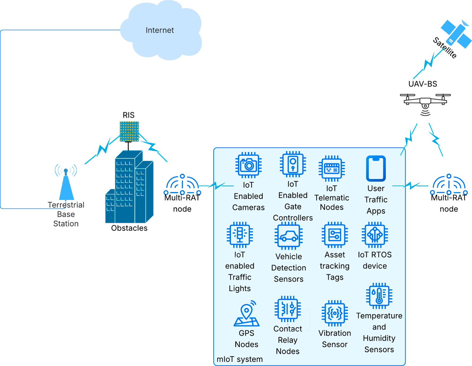
Figure 1: Network architecture.

The set of edges E={e1,e2,…,el} represents all the connections in the UDG, where l = |E|. On the second layer, multi-RAT nodes are responsible for forwarding the received packets to the 6G BS if they are destined remotely for the cloud servers or locally if they are destined for the edge servers. Multi-RAT are smart, unified access nodes that can communicate over both 6G cellular (e.g., sub-THz, THz frequency bands) and Wi-Fi (e.g., Wi-Fi 6/6E/7) to seamlessly connect IoT nodes to the 6G network and support local edge computing. In addition, they provide IPv4/IPv6 and protocol translation, offer seamless switching between Wi-Fi and 6G, and support edge intelligence, including mobility prediction, routing, and caching. The third layer hosts the base stations, which bridge 6G connectivity between multi-RAT nodes and 6G terrestrial and non-terrestrial networks. IRS units may also exist to extend 6G coverage by providing a virtual non-line-of-sight (NLoS) path between BS and multi-RAT nodes.

3.2 The Distributed-Connected Dominating Set Algorithm Based on Two-Hop Information and Expansion Nodes (D-CDS-TE)

This section introduces a heuristic distributed greedy algorithm that classifies IoT nodes to create a virtual backbone. It is formed based on the exchanged one- and two-hop information and the selection of expansion nodes, which will be explained shortly. The virtual backbone is the union of the DS and C sets, where DS is the set of independent nodes, DS={d1,d2,…,dx}, x=|DS|, and C is the set of connecting nodes, where C={c1,c2,…,cy}, y=|C|. The distance between any two nodes in the DS set is at least two hops. Any node that is not included in the CDS is at most one hop away from at least one CDS node. Accordingly, any node may forward its packets to the nearest CDS node. It will, in turn, relay the packet to the next CDS node until it reaches its destination locally in the mesh network or the nearest multi-RAT node if it is destined remotely for edge or cloud servers. Forwarding packets to the multi-RAT node is performed in the event of poor or no 6G coverage.

The D-CDS-TE algorithm classifies nodes into four main states, namely the dominator state, the sub-dominator state, the intra-connector state, and the dominatee state. Each main state has two sub-states, which are the probable sub-state and the definite sub-state. If the node is in a probable sub-state, it may change its main state based on the information it collects from its neighbors. Once a node is in a definite sub-state, it cannot return to the probable sub-state. The CDS consists only of the nodes in their definite states, namely the dominator, intra-connector, and sub-dominator. However, a node in the definite sub-state may also be selected as an interconnector. The dominator selects the interconnector nodes after the definite states of all nodes in the cluster are determined. The interconnector is also a CDS node. The color code that represents nodes’ states is as follows. Probable state dominators and probable state sub-dominators are blue nodes, black nodes represent the definite state dominators, and red nodes are the definite state sub-dominators. Intra-connector nodes are colored yellow whether they are in the probable or definite sub-states. Similarly, green is also used to indicate definite and probable dominant nodes. Finally, the purple-colored nodes are the interconnector nodes. Each cluster is typically formed of one dominator, which is the root of the cluster sub-CDS tree, and a number of sub-dominators and intra-connectors. Intra-connectors link the dominator and sub-dominators with each other.

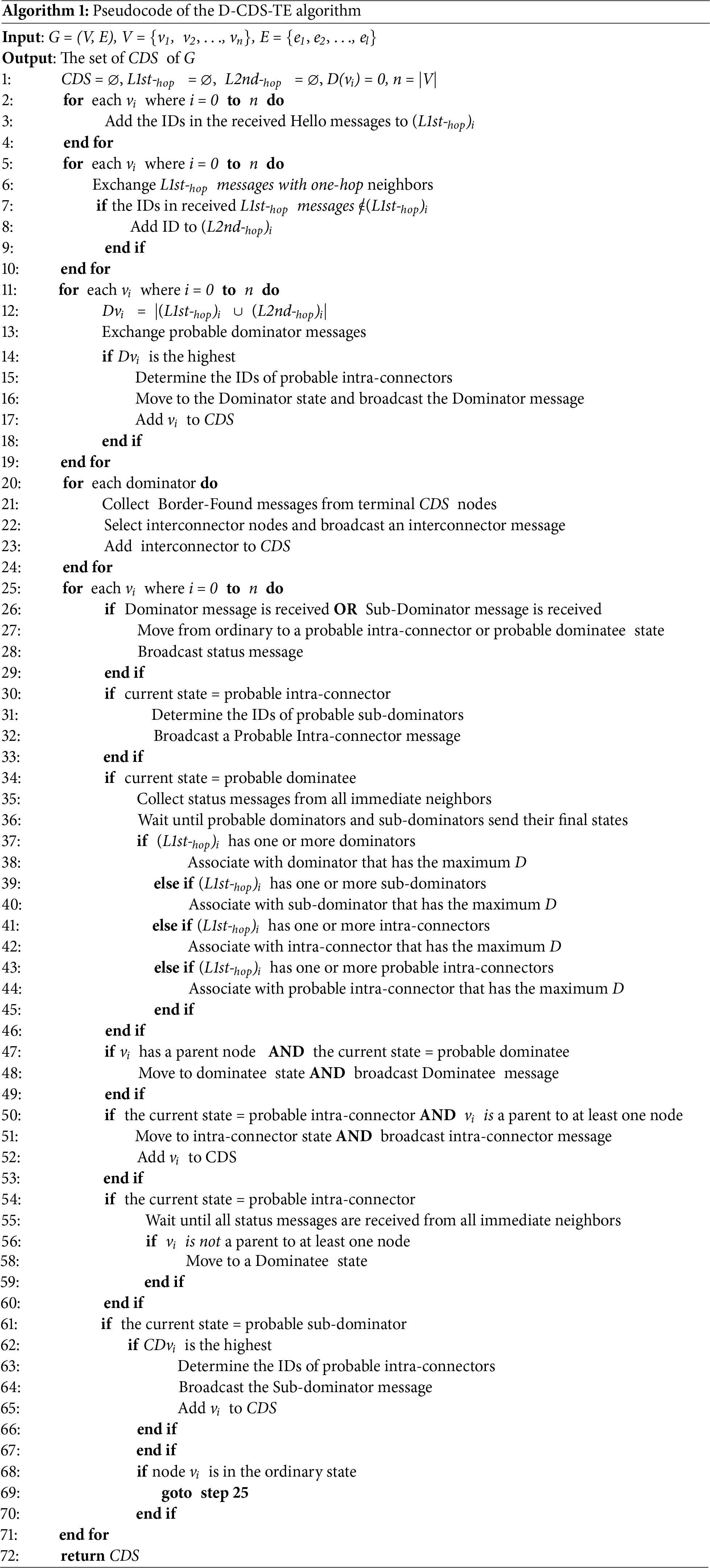
The CDS algorithm is executed by each node in the network. Initially, all nodes are in the ordinary state. The algorithm starts with ordinary nodes exchanging Hello messages to create the one-hop neighbors list (L1st-hop) for each node in V. After the list is finalized, ordinary nodes exchange L1st-hop. Hence, each node uses the collected lists to create the two-hop neighbors list (L2nd-hop). The total degree D of node v is Dv = |L1st-hop ∪ L2nd-hop|. After calculating D for each node, it enters a probable dominator state, and the node color is changed to blue. Each node broadcasts its total degree value to its one-hop neighbors. This information is also relayed to its two-hop neighbors. The node with the highest D among its two-hop neighbors changes its state to a definite dominator. It is a black node, and its level in the cluster tree is one. The node with the smaller D returns to the ordinary state. A black node broadcasts the Dominator message to its one-hop neighbors, which contains its ID, level, color, state, the IDs of the probable intra-connectors, L1st-hop, L2nd-hop, and the ID of the cluster. One-hop neighbors, which were not selected as probable intra-connectors, become probable dominatees. The dominator selects its probable intra-connectors by determining the cluster expansion nodes from the set of its one-hop neighbors. The mechanism used to find the set of cluster expansion nodes is explained shortly. Each node that receives the Dominator message assigns the black node as its dominator, increases its level by one, and changes its state and color. Probable intra-connector nodes are colored yellow, and probable dominatee nodes are colored green. Each node in the CDS has a dominator except the black node, which represents the head of the cluster.

Nodes, which received the Dominator message, broadcast either the Probable Intra-connector message or the Probable Dominatee message to all their one-hop neighbors. The Probable Intra-Connector message contains the sender ID, its level and color, the cluster ID, the sets L1st-hop and L2nd-hop of its dominator, and the IDs of probable sub-dominators, which are the determined expansion nodes. One-hop neighbors, which were not selected as probable sub-dominators, become probable dominatees. Nodes that received the Probable Intra-Connector message broadcast either the Probable Sub-Dominator message or the Probable Dominatee message to all their one-hop neighbors. The Probable Sub-dominator message contains the sender ID, cluster ID, its level, and the degree of its contribution to the cluster. The Contribution Degree (CD) of sub-dominator u is CDu = |(L1st-hop)u − (L1st-hop ∪ L2nd-hop)w|, where w is the ID of the dominator of the intra-connector. The node with the highest CD among its peers continues to collect replies from its one-hop neighbors. Other probable sub-dominator nodes with lower CD return to the ordinary node state. Once the probable sub-dominator node that has the highest CD collects replies from all its one-hop neighbors, it changes its state to definite sub-dominator and broadcasts the Sub-Dominator message. The message carries its ID, level, color, state, the ID of its dominator, its L1st-hop and L2nd-hop, and the IDs of the probable intra-connectors.

Any intra-connector that receives a sub-dominator or a dominatee message, which has its own ID in the dominator field, changes its state to a definite intra-connector and broadcasts the intra-connector message. After collecting the replies from all its neighbors, if a probable intra-connector node finds that it is not a dominator of any node, it changes its state to a definite dominatee and broadcasts the Dominatee message. The Dominatee message carries the ID of the sender, its level, color, state, and the ID of its dominator. To move from the probable dominatee state to the definite dominatee state, the node collects the replies from status messages sent by all its one-hop neighbors. The node may associate itself with another dominator. This association is determined according to the dominator priority, as shown in the algorithm flowchart in Fig. 2. Any cluster typically consists of one dominator (black node), zero or more intra-connectors (yellow nodes), zero or more sub-dominators (red nodes), and one or more dominatees (green nodes). The D-CDS-TE algorithm pseudocode is presented in Algorithm 1.

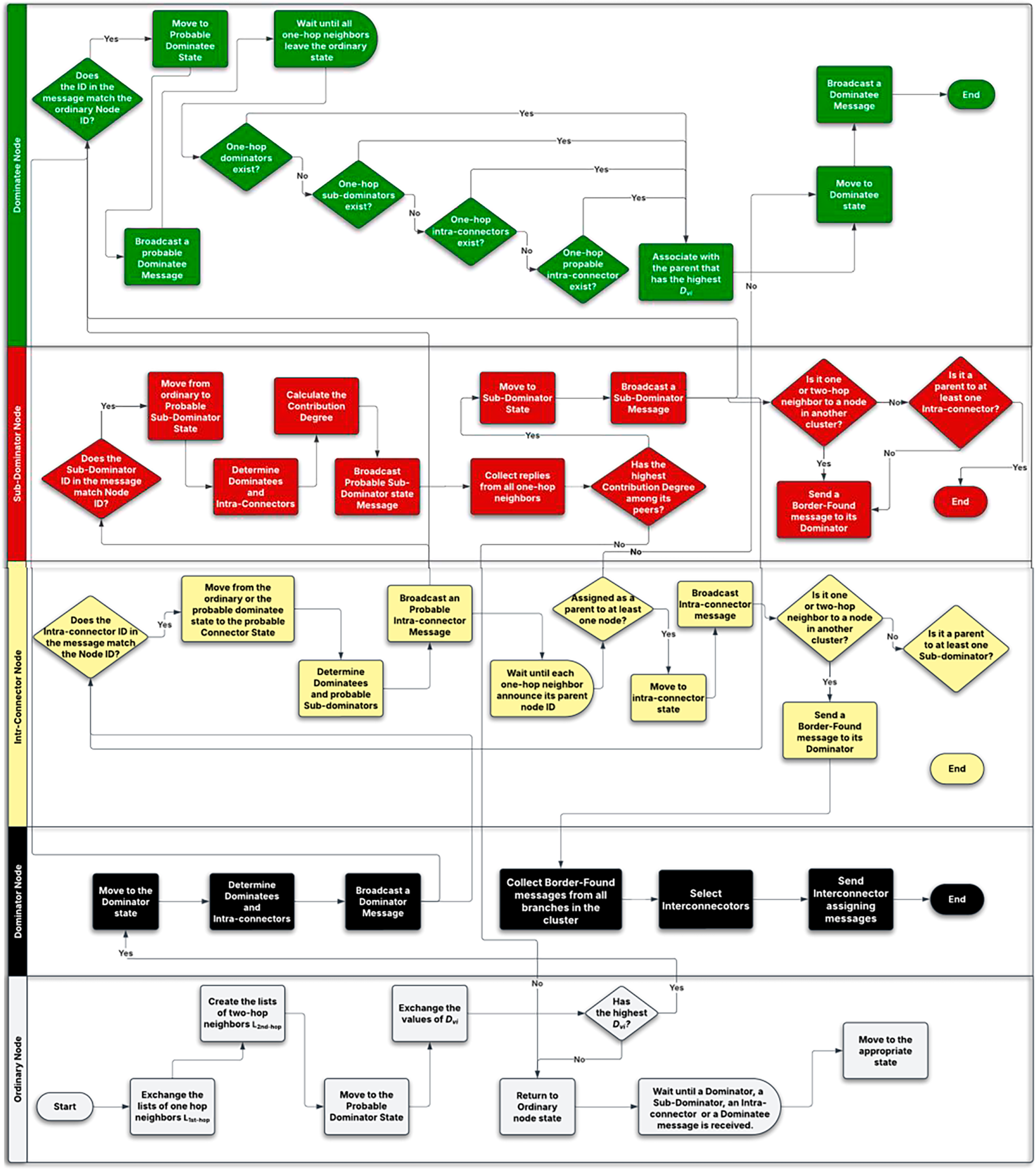
Figure 2: The D-CDS-TE algorithm flowchart.

The chain of CDS nodes connects all nodes in the cluster. Accordingly, any green node in the CDS is at most one hop away from at least one black, yellow, or red node. Once the node state is determined as a definite dominator, sub-dominator, or probable intra-connector, it determines the cluster expansion nodes from the set of its one-hop neighbors. Those nodes can be assigned either as intra-connectors or sub-dominators according to the node performing the calculations. The cluster expansion nodes can be identified as follows:

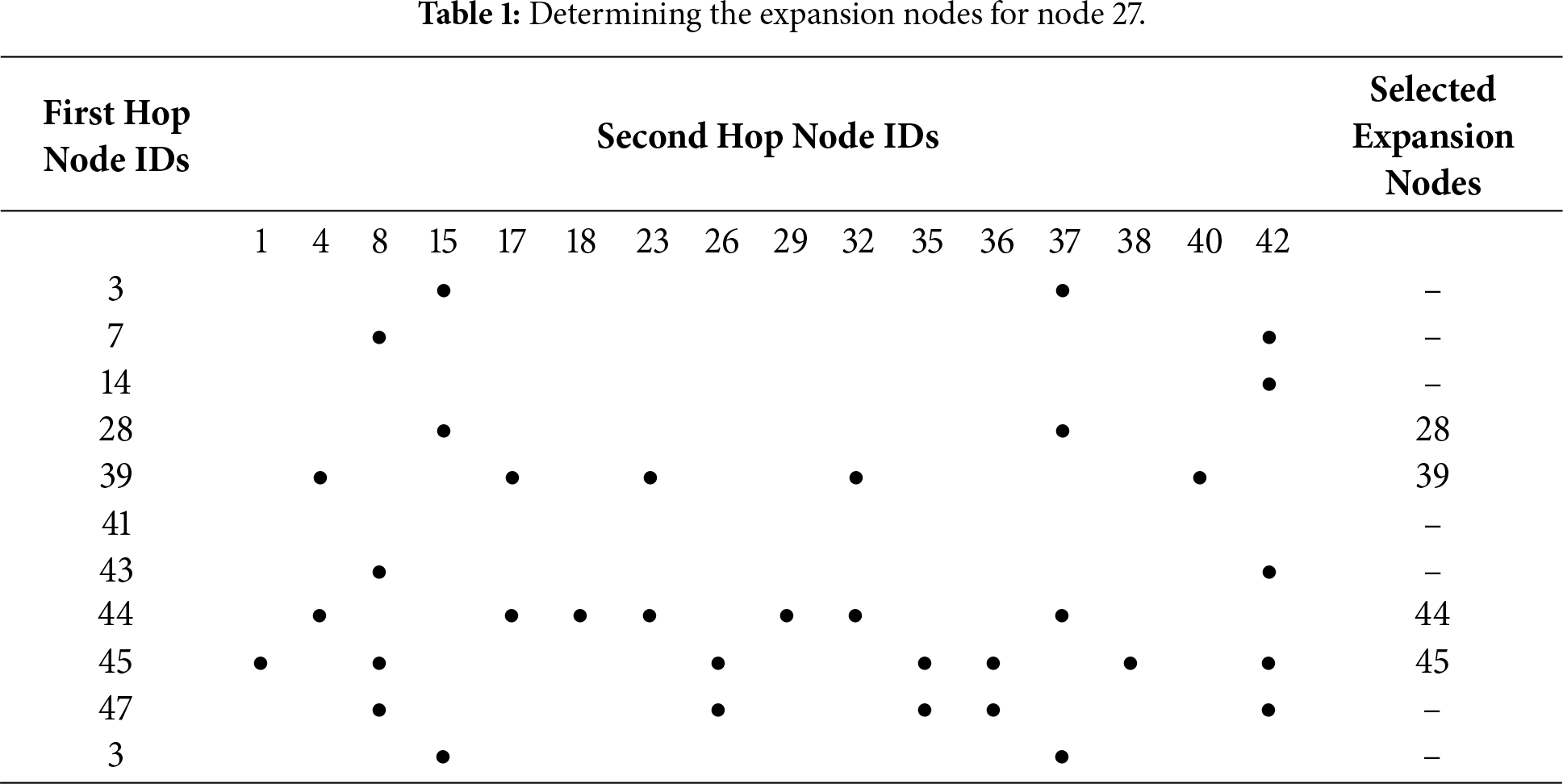
•   Every black, yellow, or red node creates a two-dimensional matrix. The IDs of the rows are the IDs of its one-hop neighbors, and the IDs of the columns are the IDs of its two-hop neighbors without repetition, as shown in Table 1.

•   For each row, the cell in the row is filled if the ID of the column is a one-hop neighbor to the ID of the row. The matrix can be traversed either horizontally or vertically. Both methods lead to the same result.

–   Horizontally, a black, yellow, or red node finds the row with the highest number of filled cells and marks them. The ID of that row is the ID of the first expansion node. In the case of a tie, the row with the highest ID wins. Columns that have marked cells are excluded from the next round of calculations. In the subsequent round, the unexcluded columns are traversed row by row to find the next expansion node. The process ends when each column has at least one marked cell.

–   Vertically, a black, yellow, or red node selects the column with the lowest number of filled cells and marks them. The node selects the ID of the corresponding row with the highest number of filled cells to be its first expansion node. In the case of a tie, the row with the highest ID wins. All filled cells in that row are marked. Columns that have marked cells are excluded from the next round of calculations. In the subsequent round, the unexcluded columns are traversed vertically. The process ends when each column has at least one marked cell.

•   Fig. 3 illustrates an example of this process. Node 27 is connected to 10 one-hop neighboring nodes and 16 two-hop neighboring nodes, and Table 1 is filled accordingly. Nodes 44 and 45 have the largest number of filled cells, which is 7. Node 45 has the highest ID; hence, it is selected as the first expansion node. Columns 1, 8, 26, 35, 36, 38, and 42 are now marked. From the set of unmarked columns, which are 4, 15, 17, 18, 23, 29, 32, 37, and 40, node 44 still has the highest number of unmarked columns; hence, it is selected as the second expansion node. Now the only unmarked columns are 15 and 40. Nodes 3 and 28 both have the same number of unmarked columns, which is 1. Hence, node 28 is selected as the third expansion node because its ID is higher than node 3. Now all columns are marked except for column 40. Accordingly, node 39 is selected as the last expansion node.

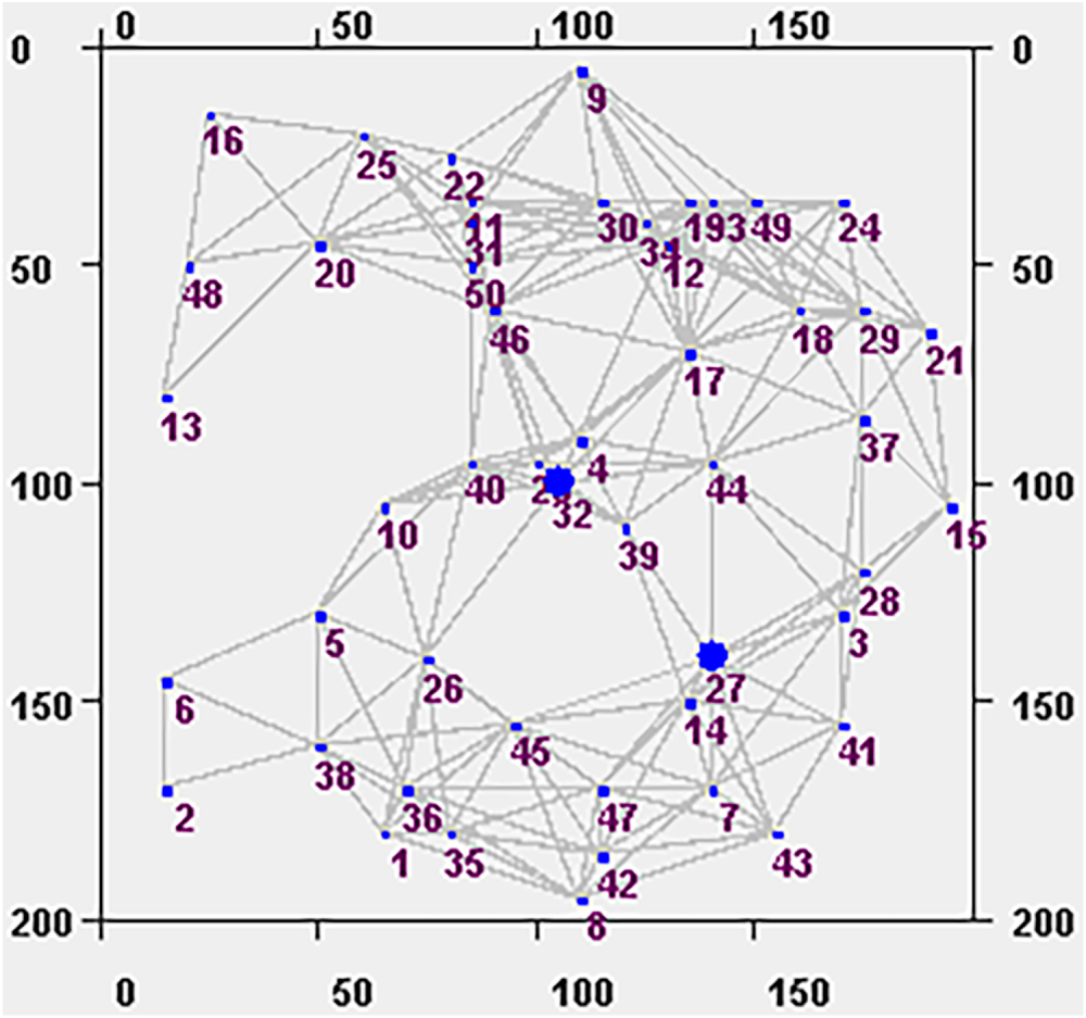
Figure 3: A random node distribution in a 200 m×200 m network shows Node 27 and its one-hop and two-hop neighbors.

In the D-CDS-TE algorithm, any node could determine its state based on the one-hop or two-hop data collected from its neighbors. No global-cluster information is exchanged or required to enable the formation of clusters. Fig. 4 illustrates the progress of the D-CDS-TE algorithm to select the virtual backbone nodes. The example shows a 200 m×200 m network area hosting 100 nodes with 50 m of transmission range. Fig. 4a shows the network after the selection of the definite dominator, which is node 57. In Fig. 4b, Node 57 has sent the Dominator message to its one-hop nodes. Hence, the state of those nodes changed to either probable intra-connector or dominatee nodes. Intra-connector nodes 14 and 18 sent their probable intra-connector messages, as shown in Fig. 4c. Hence, the receiving nodes change their states to either probable-sub-dominator or dominatee. In Fig. 4d,e, more connectors have sent their probable intra-connector messages, the probable sub-dominators compete, and the node with the highest CD wins. The definite sub-dominator node 58 sent the Sub-Dominator message, and the receiving nodes changed their states, accordingly, as shown in Fig. 4f. Intra-connector nodes that are not parents of any nodes change their state from probable intra-connector, as shown in Fig. 4g, to define dominatee nodes as shown in Fig. 4h. The final virtual backbone is presented in Fig. 4i, which has 15 CDS nodes.

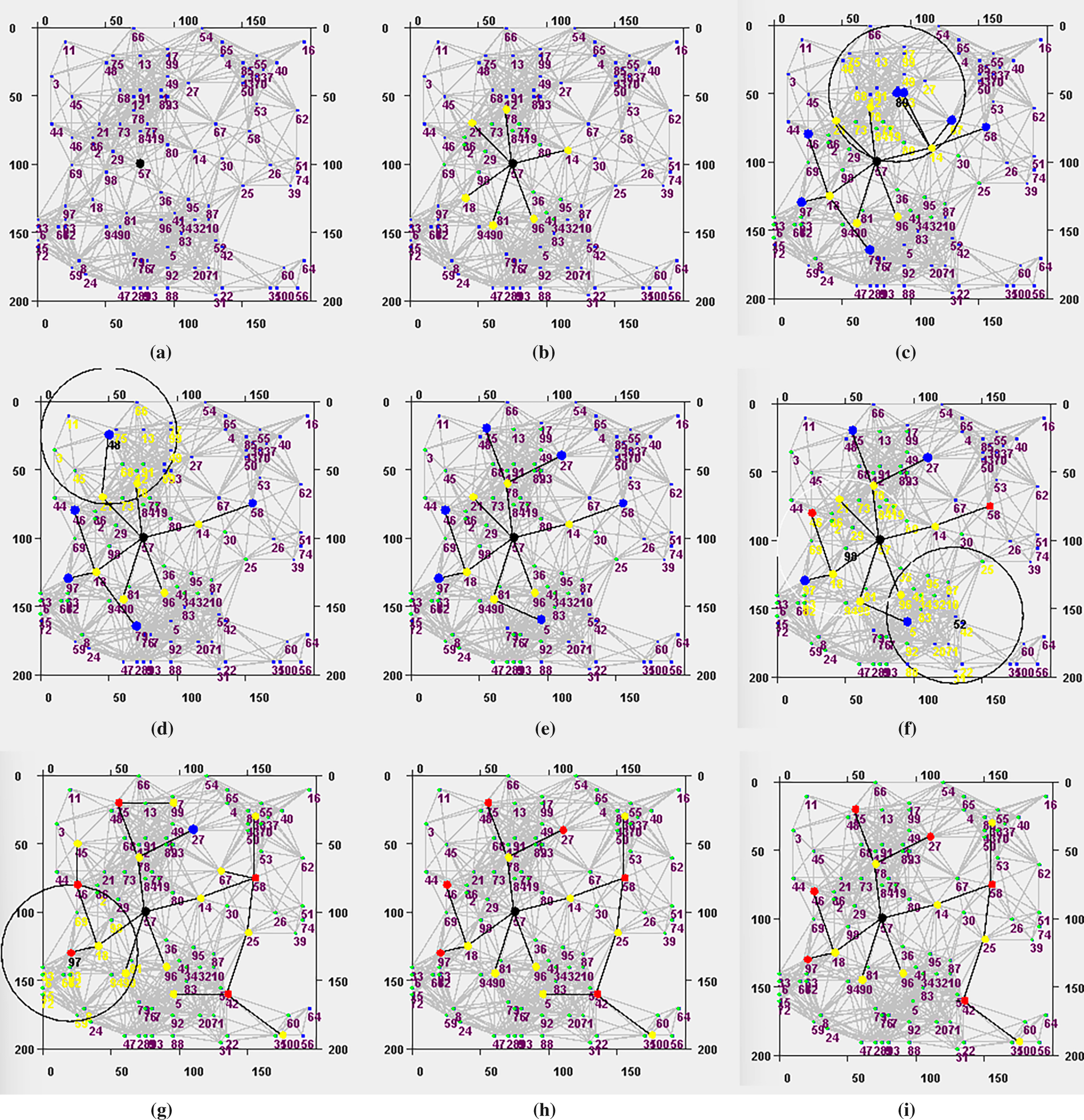
Figure 4: Example of selecting CDS nodes in 200 m×200 m network area hosting 100 nodes with 50m transmission range: (a) Node 57 is the dominator; (b) Probable intra-connectors are determined; (c) Probable sub-dominators compete; (d) Probable sub-dominator with the a lower CD return to ordinary state; (e) The rest of the probable sub-dominators are determined; (f) Nodes 46 and 58 determine their state as sub-dominators; (g) The next set of probable intra-connectors are determined; (h) Probable intra-connectors with no descendants move to dominatee state; (i) The virtual backbone is formed.

3.3 Correctness of the D-CDS-TE Algorithm

Theorem 1: The D-CDS-TE algorithm creates a CDS in which each dominatee is at most one hop away from at least one node in the CDS.

Proof of Theorem 1: The first part of this proof illustrates the correctness of the CDS structure. First, the D-CDS-TE algorithm determines the dominator nodes. The dominator node is the one that has the highest D among its two-hop neighbors. Accordingly, each dominator is at least two hops away from any other dominator in the network. Second, each dominator determines its one-hop intra-connectors. Those intra-connectors select the sub-dominators from the list of their one-hop neighbors. If two or more sub-dominators are found to be one-hop neighbors, the node with the highest CD wins, and the other node returns to the ordinary state. Accordingly, no two sub-dominators could be less than two hops apart. After receiving Border-Found messages from all its terminal cluster nodes, the dominator selects the interconnector nodes from the set of its CDS. A dominatee may be selected as an interconnector and join the CDS if there are no immediate CDS neighbors that have links to the other clusters. Based on the created topology, all dominators and sub-dominators are at least two hops apart, and each of them is connected to the CDS by at least one connector. Connectivity of the CDS relies on two elements. The first element is the existence of expansion nodes, which is guaranteed by the existence of two-hop neighbors. In a low-density network, nodes may have only one-hop neighbors. Accordingly, they do not have expansion nodes, and the value of D is the node’s degree. The second element is the ability for the node to change its main state if it is in the probable substate. Hence, the connectivity of CDS is guaranteed.

Dominatee nodes are determined based on the status messages they received from their one-hop dominators, sub-dominators, or intra-connectors. Those messages are not relayed by any other node. Hence, any dominatee must be at most one hop away from at least one CDS node. □

3.4 The D-CDS-TE Algorithm Approximation Ratio

Theorem 2: The approximation ratio of the algorithm is at most 2.06748 (3.4306 MCDS + 4.8185).

Proof of Theorem 2: A tighter expression between the Maximal Independence Set (MIS) and the Minimum Connected Dominating Set was presented in [28]. The authors proved that the size of the MIS ≤ 3.4306 MCDS + 4.8185 [28]. To compute the algorithm approximation ratio, the maximum number of independent nodes is calculated for concentric disks with radii 2R, 4R, 6R, …, (2R) m, where R is the transmission range and m is the ordinal number of the disk. The problem of selecting those nodes in a UDG is NP-complete [29]. To calculate the maximum number of independent nodes selected by the D-CDS-TE algorithm, the disk is represented as an inscribed circle in a square area network in which nodes are distributed randomly with ultra-high density.

A 2R-radius disk is a two-hop area network. This network could only have one dominator, which is the node at the disk center. That is because this node is the one with the highest D. A probable sub-dominator wins if it has the highest CD among its one-hop neighboring peers. A node would have the highest CD if it were located as far as possible from its parent node (i.e., the intra-connector node). All intra-connectors that are not parents to any node change their states to dominatee nodes. Accordingly, the Euclidean distance between the intra-connector and any node of its sub-dominators is R. In a 2R-radius disk, the maximum number of CDS nodes is 23. This is true if Lemma 1 is correct. □

Lemma 1: In a two-hop area network, the highest number of connectors or sub-dominators cannot exceed 11.

Proof of Lemma 1: In Fig. 5, θ=sin−1⁡(R+Δ)2R, if Δ=0, then the Euclidean distance between any two adjacent centers is R and θ=30∘. This gives a total of 12 non-independent nodes. Hence, in one cluster, the maximum number of sub-dominators that are two hops away from the dominator is 11. In the worst case, each intra-connector is a parent to at most one sub-dominator. Accordingly, the maximum number of intra-connectors is 11. Even if the number of probable intra-connectors is greater than 11, probable dominatee nodes will associate themselves with the definite intra-connectors because they have higher priority than probable intra-connectors. Accordingly, probable intra-connectors change their state to probable dominatees. This limits the maximum number of intra-connectors to 11. By adding the dominator node, sub-dominators, and intra-connectors, the maximum number of CDS nodes that cover a disk with radius 2R is 23 nodes. □

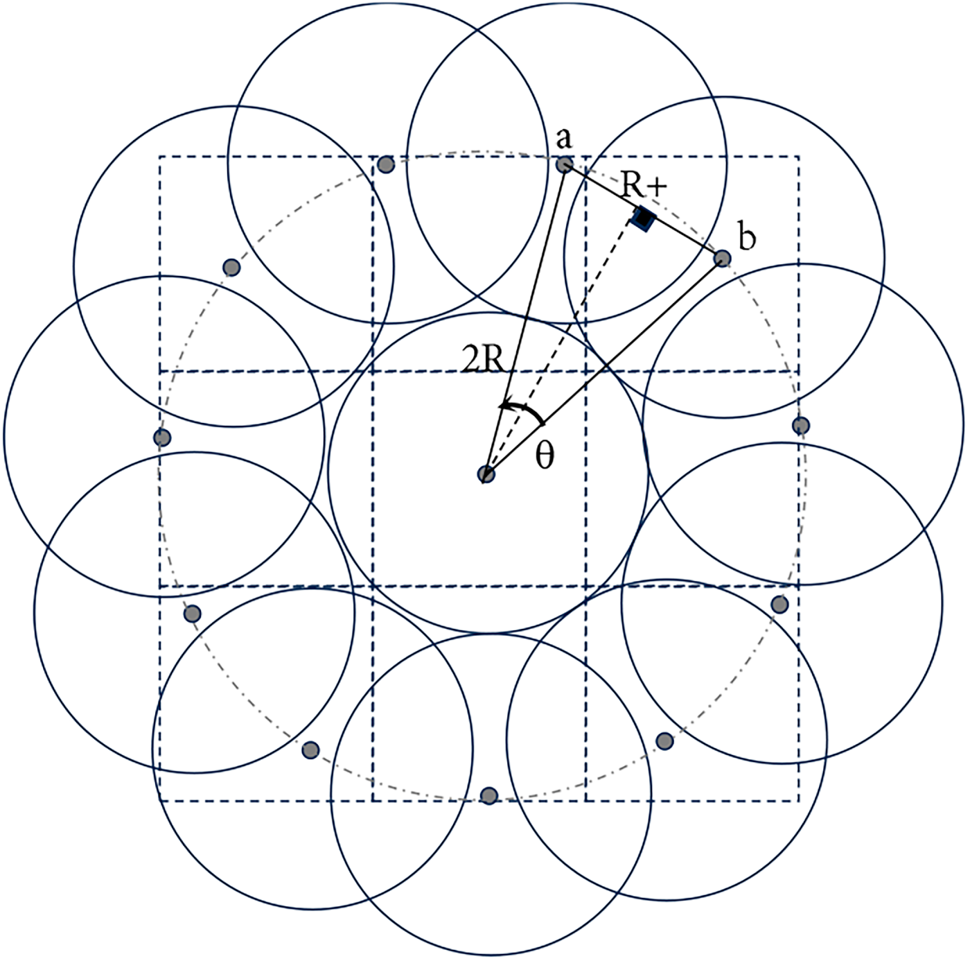
Figure 5: The maximum number of intra-connectors and sub-dominators for a dominator node in a too dense network.

For higher (2Rm)-radius disks, the area where dominators may appear is in the dominators’ region, as shown in Fig. 6a–e. Lower D values occur as the node approaches the network edge because, in the case of uniformly distributed nodes, the node inside the dominator region has its two-hop circular area falling entirely in the network, whereas nodes outside the dominator region have a fraction of their two-hop radius falling inside the network area. Hence, the sides of the dominator region are always distant by 2R from corresponding sides of the square area network. Dominators are expected to appear in this region because the nodes in this area have higher D values than the nodes outside that region. Each increment in m increases the side length of the inner square by 4R, as shown in Fig. 6b. At an 8R-radius disk, the inner square intersects the inscribed circle, as shown in Fig. 6c. That is because the diagonal length of the dominators’ region is 22(2R(4−1))2=122R, which is greater than 16R. As the disk diameter increases, the intersection area between the inner square and the inscribed circle increases, as shown in Fig. 6d. Fig. 6e illustrates that ∠∅=2cos−1(m−1m) and when m→∞,∠∅=limm→∞2cos−1(1−1m)=0∘, which means that the dominator region would completely cover the disk area.

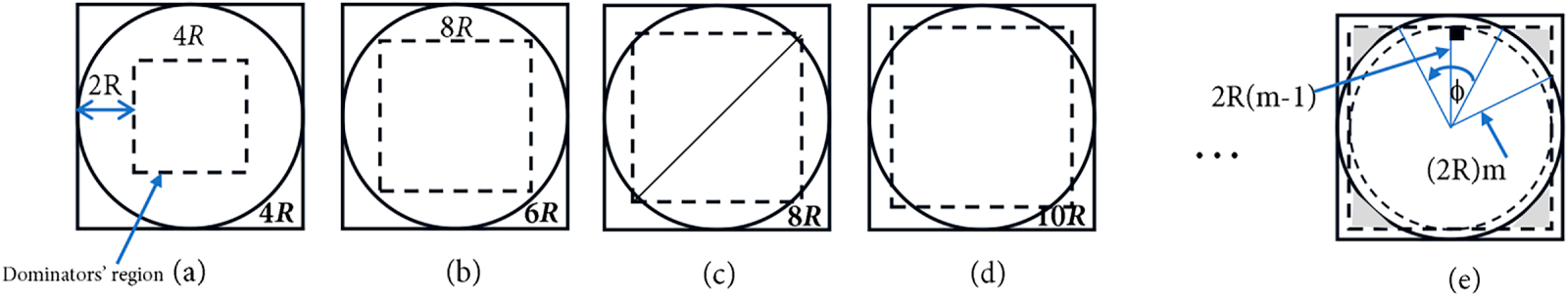
Figure 6: The relation between the dominator region and the disk area as the value of m increases: (a) Disk radius is 4R; (b) Disk radius is 6R; (c) Disk radius is 8R; (d) Disk radius is 10R; (e) Disk radius is 2Rm.

To pack the maximum number of dominators in the grey region, the distance between any two-hop adjacent dominators is at least 2R, as shown in Fig. 7. The value that determines the dominator increment pace is as follows:

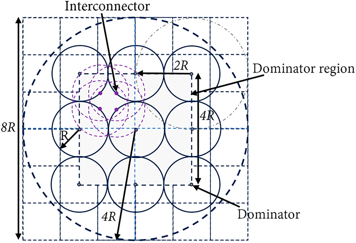
Figure 7: The maximum number of dominators in an 8R square area network.

For a 4R-radius disk, starting at the top left corner of the grey region, if the distance between two adjacent dominators is 2R, then the maximum number of dominator nodes is nine, as shown in Fig. 7. With each increment in the value of m, the number of dominators is increased by two on each side. Hence, it can be concluded that, for higher m values, the maximum number of dominators is (2m − 1)2. To achieve full connectivity among clusters, each dominator could select up to four nodes to connect to its neighboring dominators. In a 4R-radius disk, where m = 2, the maximum number of interconnectors is 16. For higher m values, the number of interconnectors is 4(2m − 2)2.

For low m values, dominators cannot fully cover the disk area. Accordingly, each dominator would have a number of sub-dominators to cover the disk circumference. For m = 2, 4R-radius disk, the maximum number of sub-dominators is 23. Sub-dominators can possibly exist for dominators positioned at the perimeter of the grey region. Based on Lemma 1, this time θ=sin−1⁡(R+Δ)4R, if Δ=0, then the Euclidean distance between any two adjacent centers is R and θ=14.447∘. This gives a total of 24 adjacent R-radius nodes and one node with a transmission range of 0.433R. To ensure that those sub-dominators are independent, at most 23 nodes can coexist in this constellation. Similarly, assuming that each intra-connector is a parent to at most one sub-dominator, the number of intra-connectors is 23. Hence, the maximum number of CDS nodes that cover a disk with radius 4R is 71 nodes, which consists of 9 dominators, 16 interconnectors, 23 sub-dominators, and 23 intra-connectors. For low m values, the CDS size = (2m − 1)2 + 4(2m − 2)2 + 2(2π/θ − 1). As the value of m is increasing significantly, the number of sub-dominators required to cover the disk is starting to decrease because the dominators are covering more of the disk area. For very high m values, the CDS size = (2m − 1)2 + 4(2m − 2)2. For a disk with diameter 2 m, the least economical convex sets for lattice covering is (2π3/9)2 m2 [30]. The authors in [31] proved that the previous equation is correct if the connection angle (r) ≤ (π/3) [31]. The connection angle is the central angle associated with the connection chord between two intersecting transmission ranges of two adjacent nodes. As the connection angle increases (i.e., r > (π/3)), the required number of independent nodes that cover a specific disk increases. To compare the size of the D-CDS-TE algorithm-generated CDS to the optimal MCDS, it is assumed that the nodes in the optimal DS have the value of r ≤ (π/3). This is the worst-case scenario for the proposed D-CDS-TE algorithm. If each independent node in the optimal DS associates to the MCDS using one connector, the approximation ratio of the D-CDS-TE algorithm when m → ∞ is:

limm→∞(2m−1)2+4(2m−2)22(2π/33)(2m)2(1)

limm→∞20m2−36m+179.6736m2=2.06748(2)

Hence, the algorithm approximation ratio is 2.06748 (3.4306 MCDS + 4.8185). □

3.5 Time and Message Complexities

Primarily, more than one cluster may exist in the network area based on the ratio between the network dimension and the transmission range. The cluster creates its virtual backbone by adding new CDS nodes until there are no more CDS nodes to include. This may occur because of one of two reasons. First, the current CDS node does not have potential CDS candidates because it is a terminal node at the edge of the network. Second, all its potential CDS candidates have already joined another cluster. In either case, this branch cannot expand further, and the CDS node sends a Border-Found message to the cluster dominator. The dominator collects those messages from all its virtual CDS branches and then broadcasts the interconnector message, which is relayed to the CDS nodes that previously sent the Border-Found message. The message has the IDs of the interconnector nodes and the IDs of the neighboring clusters they connect to. This guarantees that all CDS nodes in the cluster are aware of their surroundings. In a unit disk graph, assuming that the farthest CDS node is K hops away from the cluster dominator. Hence, K represents the depth of the cluster, where the number of hops between the dominator and any other CDS node in the cluster cannot exceed K. As a result, at most K rounds are required to establish the cluster, K rounds to relay the Border message to the Dominator, and K rounds to deliver the Interconnector message to the terminal CDS nodes. Accordingly, the time complexity of the algorithm is O(K). In a one-cluster network, the maximum distance between any two CDS nodes is at most 2K, and the farthest distance between any two dominatee nodes cannot exceed 2(K + 1). Hence, in a single cluster network, the network diameter D has an upper limit, which is 2(K + 1). Because each node is required to send a finite number of messages according to its role or state in the cluster, and no node can remain in the ordinary state indefinitely after a finite number of exchanged messages, every unit in the network will reach its definite state. Hence, the message complexity of the algorithm is O(n).

4  Discussion

Several recent studies [18,19,26] focused on evaluating the performance of the presented CDS algorithms in two-hop or less area networks, where the ratio between the transmission range and network side length is 25% or more. Therefore, one cluster on average is usually formed inside the network area. As far as the author knows, the larger networks with a higher number of clusters were not investigated thoroughly. In this section, the CDS size resulting from the D-CDS-TE algorithm is evaluated in two- and four-hop square area networks. Moreover, it is also compared against the theoretical optimal limit to the size of the CDS in a two-hop square area network, which is derived in Theorem 3.

Theorem 3: The minimum number of CDS nodes with transmission range R that can form a virtual backbone in a square area network with side length 4R is 13.

Proof of Theorem 3: To determine the minimum number of independent nodes that could cover a square network area of side length 4R, the circles created by the transmission range R should be overlapped without violating the independence conditions (i.e., the distance between the centers of any two independent nodes is greater than R). By splitting the network area into nine equal square cells, the side length of the cell is 4/3R. The maximum square area that can be covered by node j with radius R is 2R2, which is larger than the cell area 16/9R2. Hence, nine DS nodes can completely cover the network area with a side length 4R. Because each node is positioned at the center of the cell, the Euclidean distance between any two adjacent nodes is 4/3R; hence, the independent condition holds. If it is impossible to verify that eight nodes with equal radii R can completely cover a 16R2 network region, then nine nodes are the lowest number that provide this coverage, as illustrated in Fig. 8. Using the simulated annealing approach, the authors in [32] proved that the minimum number of circles that can completely cover a square area is eight if the ratio between the side length and the circle radius does not exceed 3.84172. Because the ratio between the network side length and the transmission range is 4, it is impossible for eight nodes to totally cover the network area. □

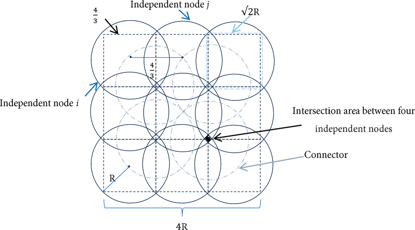
Figure 8: The minimum number of CDS nodes in a two-hop square area network is 13.

To create the virtual backbone, the minimum number of connectors should be determined, too. Nodes in the intersection areas are suitable candidates to be chosen as connectors. As shown in Fig. 8, the maximum number of intersecting circles is four, and there are four intersecting areas in the figure. Accordingly, four connectors are the minimum number of nodes that can achieve connectivity between the independent nodes. This gives a total of 13 R-radii nodes to be the optimal CDS size that can cover a 16R2 square area network. When comparing the optimal CDS size, which is 13 nodes, against the maximum number of CDS nodes that could be created by the D-CDS-TE algorithm, which is 23 nodes, as proven in Lemma 1, the ratio is 23/13 in an extremely dense two-hop square area network.

In simulations, the size of the generated CDS is studied in a two-hop square area network. For a 25 m transmission range, the network is. Nodes are identical and randomly distributed on the network area with varied n values from 25 to 300. Each average CDS size is computed after 10 runs. The simulator, presented in [33], is used to execute the simulations. Simulation parameters are presented in Table 2. Results show that for 25 nodes, the average CDS size is 10.7, and it increases to 16.2 when n reaches 300 nodes, as shown in Fig. 9.

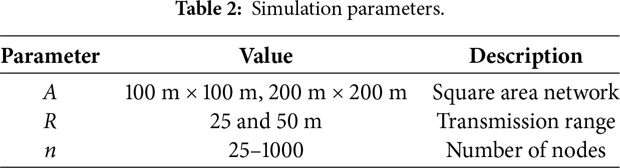
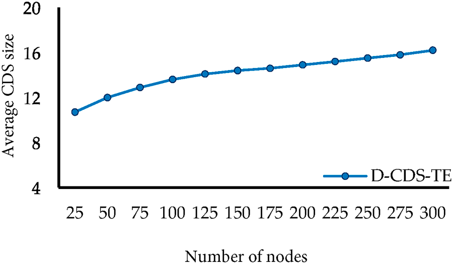
Figure 9: The average CDS size in A = 100 m×100 m, and R = 25 m.

To investigate the effect of interconnectors on the CDS size, a four-hop square area network is selected to conduct simulations. Simulations were performed using varied node populations of 200–1000 nodes, as shown in Fig. 10. The corresponding average CDS size varies from 58.2 to 69.3. The CDS curve has a small positive average slope that equals 0.014, which indicates efficient adaptation to the increase in the number of nodes. The size of the CDS is approximately 7% of the total number of nodes when n reaches 1000 nodes. Hence, having several clusters inside the network did not degrade the algorithm performance.

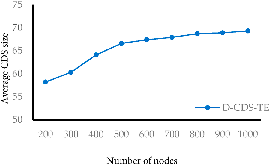
Figure 10: The average CDS size in A = 200 m×200 m, and R = 25 m.

Simulation results of various CDS algorithms are compared against the performance of the D-CDS-TE algorithm in a two-hop network. Both centralized and distributed algorithms are included in the comparison. The BD-ECDS algorithm in [18] consists of two phases. The first phase creates the DS, and the second phase selects the connectors. The DCMCDS algorithm in [19] presented an improved breadth-first search algorithm to construct the DS. The main limitation of this approach is the high number of rounds required to create the tree. Scalability is a main challenge that hinders the practicality of deployment in larger networks. Two CDS algorithms are presented in [26]. In both algorithms, the selection of DS is performed using a centralized algorithm, which is challenging as the size of the network increases. Fig. 11 compares the size of the CDS algorithm against the BD-ECDS [18], DCMCDS [19], IK-ST, and ML-ST [26] algorithms. Although the size of the CDS is larger than the best value achieved by the IK-ST algorithm, the CDS algorithm has the lowest positive average slope. This indicates that it can handle the increase of the nodes’ density more efficiently than other algorithms, especially the IK-ST and ML-ST algorithms. Fig. 12 depicts the average slope of CDS curves for the same set of algorithms against the D-CDS-TE algorithm.

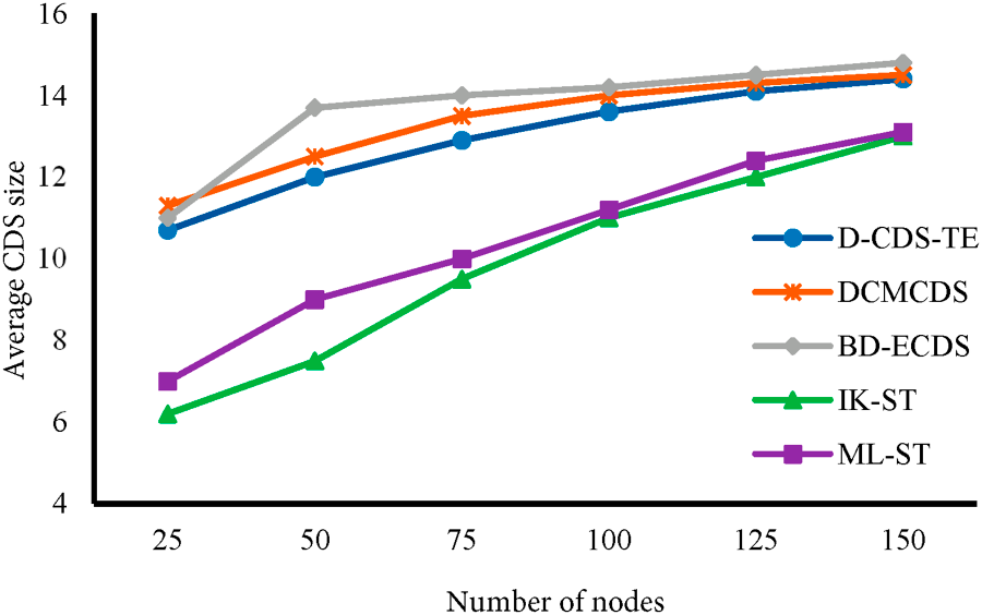
Figure 11: The average CDS size in A = 100 m×100 m, and R = 25 m.

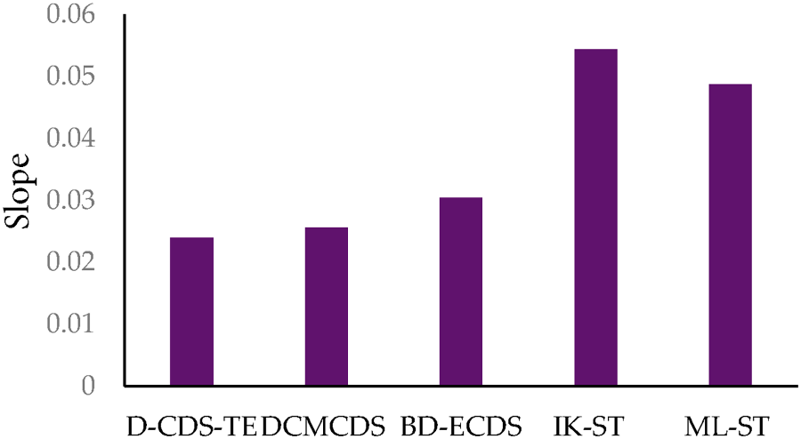
Figure 12: The average slope of the CDS curves plotted in Fig. 11.

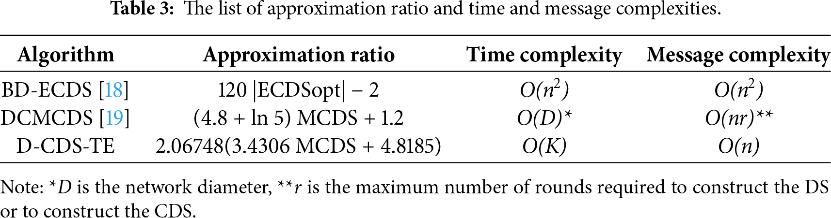
Table 3 compares the approximation ratio and the time and message complexities for BD-ECDS and DCMCDS against the D-CDS-TE algorithm. The comparison shows that the proposed algorithm has the least approximation ratio and the lowest time and message complexities. This indicates that the performance of the D-CDS-TE algorithm outperforms other algorithms, especially as the size and the density of the network increase.

5  Conclusions

This study presents a distributed heuristic CDS clustering algorithm based on exchanging two-hop neighboring information and identifying cluster expansion nodes. The approximation ratio of the D-CDS-TE algorithm is 2.06748(3.4306 MCDS + 4.8185). The CDS algorithm has the lowest time and message complexities when compared to recent CDS algorithms. The performance of the algorithm is evaluated in two-hop and four-hop square area networks. In a two-hop area network, the ratio of the theoretical worst-case CDS size created by the D-CDS-TE algorithm and the optimal CDS size is 1.769:1. Simulation results show that in two-hop area networks, the size of the resulting CDS is better than that of the BD-ECDS and BD-ECDS algorithms. Furthermore, the CDS curve of the D-CDS-TE algorithm has a lower average slope than all the compared algorithms. This indicates that D-CDS-TE adapts efficiently to low- and high-density networks. In four-hop area networks, the size of the generated CDS did not exceed 7% of the total number of nodes. Future research may attempt to modify the methodology of selecting interconnectors, which consecutively can further enhance the algorithm approximation ratio and the total size of the CDS.

Acknowledgement: The authors extend their appreciation to the Deputyship for Research & Innovation, Ministry of Education in Saudi Arabia for funding this research work through the project number RI-44-0028.

Funding Statement: Deputyship for Research & Innovation, Ministry of Education in Saudi Arabia for funding this research work through the project number RI-44-0028.

Author Contributions: The authors confirm contribution to the paper as follows: Dina S. M. Hassan: conceptualization, methodology, software, writing—original draft, project administration, funding acquisition; Reem Ibrahim Alkanhel: conceptualization, methodology, investigation, writing—original draft; Thuraya Alrumaih: investigation, validation, writing—review and editing; Shiyam Alalmaei: formal analysis, validation, writing—review and editing. All authors reviewed and approved the final version of the manuscript.

Availability of Data and Materials: Not applicable.

Ethics Approval: Not applicable.

Conflicts of Interest: The authors declare no conflicts of interest.

Abbreviations

References

1. Insights release: state of IoT 2024 [Internet]. [cited 2025 Oct 1]. Available from: https://iot-analytics.com/wp-content/uploads/2024/09/INSIGHTS-RELEASE-Number-of-connected-IoT-devices-vf.pdf. [Google Scholar]

2. IoT connections outlook [Internet]. [cited 2025 Oct 1]. Available from: https://www.ericsson.com/en/reports-and-papers/mobility-report/dataforecasts/iot-connections-outlook. [Google Scholar]

3. Gupta V, Tripathi S, De S. Green sensing and communication: a step towards sustainable IoT systems. J Indian Inst Sci. 2020;100(2):383–98. doi:10.1007/s41745-020-00163-8. [Google Scholar] [CrossRef]

4. Alsharif MH, Kelechi AH, Jahid A, Kannadasan R, Singla MK, Gupta J, et al. A comprehensive survey of energy-efficient computing to enable sustainable massive IoT networks. Alex Eng J. 2024;91:12–29. doi:10.1016/j.aej.2024.01.067. [Google Scholar] [CrossRef]

5. Rahmani H, Shetty D, Wagih M, Ghasempour Y, Palazzi V, Carvalho NB, et al. Next-generation IoT devices: sustainable eco-friendly manufacturing, energy harvesting, and wireless connectivity. IEEE J Microw. 2023;3(1):237–55. doi:10.1109/JMW.2022.3228683. [Google Scholar] [CrossRef]

6. Sheraz M, Chuah TC, Tareen WUK, Al-Habashna A, Saeed SI, Ahmed M, et al. A comprehensive survey on GenAI-enabled 6G: technologies, challenges, and future research avenues. IEEE Open J Commun Soc. 2025;6:4563–90. doi:10.1109/OJCOMS.2025.3568496. [Google Scholar] [CrossRef]

7. Mahmoud HHH, Amer AA, Ismail T. 6G: a comprehensive survey on technologies, applications, challenges, and research problems. Trans Emerging Tel Tech. 2021;32(4):e4233. doi:10.1002/ett.4233. [Google Scholar] [CrossRef]

8. Pérez-Adán D, Fresnedo Ó, González-Coma JP, Castedo L. Intelligent reflective surfaces for wireless networks: an overview of applications, approached issues, and open problems. Electronics. 2021;10(19):2345. doi:10.3390/electronics10192345. [Google Scholar] [CrossRef]

9. Wu Q, Zhang S, Zheng B, You C, Zhang R. Intelligent reflecting surface-aided wireless communications: a tutorial. IEEE Trans Commun. 2021;69(5):3313–51. doi:10.1109/TCOMM.2021.3051897. [Google Scholar] [CrossRef]

10. Iskandarani MZ. Effect of intelligent reflecting surface on WSN communication with access points configuration. IEEE Access. 2025;13(21):13380–94. doi:10.1109/ACCESS.2025.3531637. [Google Scholar] [CrossRef]

11. Mohsan SAH, Khan MA, Alsharif MH, Uthansakul P, Solyman AAA. Intelligent reflecting surfaces assisted UAV communications for massive networks: current trends, challenges, and research directions. Sensors. 2022;22(14):5278. doi:10.3390/s22145278. [Google Scholar] [PubMed] [CrossRef]

12. Khan MA, Kumar N, Mohsan SAH, Khan WU, Nasralla MM, Alsharif MH, et al. Swarm of UAVs for network management in 6G: a technical review. IEEE Trans Netw Serv Manag. 2023;20(1):741–61. doi:10.1109/TNSM.2022.3213370. [Google Scholar] [CrossRef]

13. Othman WM, Ateya AA, Nasr ME, Muthanna A, ElAffendi M, Koucheryavy A, et al. Key enabling technologies for 6G: the role of UAVs, terahertz communication, and intelligent reconfigurable surfaces in shaping the future of wireless networks. J Sens Actuator Netw. 2025;14(2):30. doi:10.3390/jsan14020030. [Google Scholar] [CrossRef]

14. Abbasi O, Yadav A, Yanikomeroglu H, Đào ND, Senarath G, Zhu P. HAPS for 6G networks: potential use cases, open challenges, and possible solutions. IEEE Wirel Commun. 2024;31(3):324–31. doi:10.1109/MWC.012.2200365. [Google Scholar] [CrossRef]

15. Giordani M, Zorzi M. Non-terrestrial networks in the 6G era: challenges and opportunities. IEEE Netw. 2021;35(2):244–51. doi:10.1109/MNET.011.2000493. [Google Scholar] [CrossRef]

16. Famili A, Atalay T, Stavrou A, Wang H. Wi-six: precise positioning in the metaverse via optimal Wi-Fi router deployment in 6G networks. In: Proceedings of the 2023 IEEE International Conference on Metaverse Computing, Networking and Applications (MetaCom); 2023 Jun 26–28; Kyoto, Japan. p. 17–24. doi:10.1109/MetaCom57706.2023.00019. [Google Scholar] [CrossRef]

17. Lee H, Park S, Yoo M, Park C, Baek H, Kim J. Convergence of 6G and Wi-Fi networks. In: Fundamentals of 6G communications and networking. Cham, Switzerland: Springer; 2023. p. 719–31. doi:10.1007/978-3-031-37920-8_28. [Google Scholar] [CrossRef]

18. Wang J, Liang J, Li Q. On construction of quality virtual backbone in wireless networks using cooperative communication. Comput Commun. 2024;228(1):107952. doi:10.1016/j.comcom.2024.107952. [Google Scholar] [CrossRef]

19. Mohanty JP, Mandal C, Reade C. Distributed construction of minimum connected dominating set in wireless sensor network using two-hop information. Comput Netw. 2017;123(1–3):137–52. doi:10.1016/j.comnet.2017.05.017. [Google Scholar] [CrossRef]

20. Kobayashi Y, Kurita K, Mann K, Matsui Y, Ono H. Enumerating minimal vertex covers and dominating sets with capacity and/or connectivity constraints. Algorithms. 2025;18(2):112. doi:10.3390/a18020112. [Google Scholar] [CrossRef]

21. Li B, Zhang X, Cai S, Lin J, Wang Y, Blum C. NuCDS: an efficient local search algorithm for minimum connected dominating set. In: Proceedings of the Twenty-Ninth International Joint Conference on Artificial Intelligence; 2020 Jul 11–17; Yokohama, Japan. p. 1503–10. doi:10.24963/ijcai.2020/209. [Google Scholar] [CrossRef]

22. Zhang X, Li B, Cai S, Wang Y. Efficient local search based on dynamic connectivity maintenance for minimum connected dominating set. J Artif Intell Res. 2021;71:89–119. doi:10.1613/jair.1.12618. [Google Scholar] [CrossRef]

23. Chen J, Cai S, Wang Y, Xu W, Ji J, Yin M. Improved local search for the minimum weight dominating set problem in massive graphs by using a deep optimization mechanism. Artif Intell. 2023;314(11):103819. doi:10.1016/j.artint.2022.103819. [Google Scholar] [CrossRef]

24. Xiao Z, Zhu C, Feng W, Liu S, Deng X, Lu H, et al. Tensor and minimum connected dominating set based confident information coverage reliability evaluation for IoT. IEEE Trans Sustain Comput. 2025;10(3):547–61. doi:10.1109/TSUSC.2024.3503712. [Google Scholar] [CrossRef]

25. Yu D, Zou Y, Zhang Y, Li F, Yu J, Wu Y, et al. Distributed dominating set and connected dominating set construction under the dynamic SINR model. In: Proceedings of the 2019 IEEE International Parallel and Distributed Processing Symposium (IPDPS); 2019 May 20–24; Rio de Janeiro, Brazil. p. 835–44. doi:10.1109/ipdps.2019.00092. [Google Scholar] [CrossRef]

26. Sun X, Yang Y, Ma M. Minimum connected dominating set algorithms for ad hoc sensor networks. Sensors. 2019;19(8):1919. doi:10.3390/s19081919. [Google Scholar] [PubMed] [CrossRef]

27. Priyadarshini RR, Sivakumar N. Cluster head selection based on minimum connected dominating set and bi-partite inspired methodology for energy conservation in WSNs. J King Saud Univ Comput Inf Sci. 2021;33(9):1132–44. doi:10.1016/j.jksuci.2018.08.009. [Google Scholar] [CrossRef]

28. Li M, Wan PJ, Yao F. Tighter approximation bounds for minimum CDS in wireless ad hoc networks. In: Algorithms and computation. Berlin/Heidelberg, Germany: Springer; 2009. p. 699–709. doi:10.1007/978-3-642-10631-6_71. [Google Scholar] [CrossRef]

29. Clark BN, Colbourn CJ, Johnson DS. Unit disk graphs. Discrete Math. 1990;86(1–3):165–77. doi:10.1016/0012-365X(90)90358-O. [Google Scholar] [CrossRef]

30. Brass P, Moser WO, Pach J. Density problems for packings and coverings. In: Research problems in discrete geometry. New York, NY, USA: Springer; 2006. p. 5–74. doi:10.1007/0-387-29929-7_2. [Google Scholar] [CrossRef]

31. Bai X, Kumar S, Xuan D, Yun Z, Lai TH. Deploying wireless sensors to achieve both coverage and connectivity. In: Proceedings of the 7th ACM International Symposium on Mobile Ad Hoc Networking and Computing; 2006 May 22; Florence, Italy. p. 131–42. doi:10.1145/1132905.1132921. [Google Scholar] [CrossRef]

32. Melissen JB, Schuur PC. Improved coverings of a square with six and eight equal circles. Electron J Comb. 1996;3(1):1–10. doi:10.37236/1256. [Google Scholar] [CrossRef]

33. Hassan DSM, Fahmy HMA, Bahaa-ElDin AM. RCA: efficient connected dominated clustering algorithm for mobile ad hoc networks. Comput Netw. 2014;75(1):177–91. doi:10.1016/j.comnet.2014.10.010. [Google Scholar] [CrossRef]