LSTM-GRU and Multi-Head Attention Based Multivariate Time Series Prediction Model for Electro-Hydraulic Servo Material Fatigue Testing Machine

1  Introduction

Accurate characterization of material fatigue properties and life assessment forms the foundation for ensuring the reliability of advanced equipment. Electro-hydraulic servo fatigue testing machines, with their high-bandwidth response, high mechanical output, and programmable loading capabilities, have become essential tools for conducting fatigue and durability tests in aerospace, automotive, wind power, nuclear engineering, and other fields [1,2]. The testing machines inherently constitute a strongly coupled, nonlinear, time-varying closed-loop mechanism-fluid-electric system. This system involves multi-physics interactions among the actuator cylinder, servo valve, hydraulic power source, loading fixture, and the material under test [3]. Under complex loading conditions like sinusoidal, random, or block spectrum loads, the system is influenced by multiple factors, including valve port nonlinearity, friction and hysteresis, oil compressibility and temperature rise effects, structural stiffness variations, and sensor drift [4,5]. This not only challenges the control precision and condition reproducibility of the testing process but also increases the difficulty of timely anomaly detection and the risk of sudden equipment failure, thereby driving up maintenance costs and reducing testing efficiency.

Therefore, the ability to accurately predict these key parameters and their evolution trends during testing enables early identification of potential anomalies in monitoring, and optimization of maintenance strategies in operations and maintenance. Such predictive capabilities not only directly enhance the stability of testing machines and the reliability of test data but also provide crucial safeguards for the safety, economy, and sustainability of reliability testing. Driven by the need, we focus on parameters prediction method for fatigue testing machines.

Traditional mechanism-based modeling approaches require in-depth study of underlying mechanisms to achieve relatively accurate predictions, and most can only monitor target objects through threshold control methods [6,7]. In contrast, data-driven methods can directly predict data trends by extracting features from historical data. In recent years, deep learning—particularly recurrent neural networks—has demonstrated advantages in temporal modeling [8–10]. Olu-Ajayi et al. achieved accurate prediction of building energy consumption through deep learning methods [11]. Among these, long short-term memory (LSTM) and gated recurrent unit (GRU) effectively mitigate gradient vanishing in long sequences through gating mechanisms and have been applied to equipment condition prediction and fault diagnosis. Fantini et al. employed GRU in hourly wind power forecasting and validated its effectiveness [12]. Tian et al. proposed a deep learning ensemble model (Deep TCN-GRU) integrating temporal convolutional networks with gated recurrent units, this model significantly outperformed existing approaches in forecasting pH and total nitrogen levels in the Kaifeng water source area of the Yellow River [13]. Mohamed et al. propose a robustness testing framework based on the φ-stress operator. By constructing a variant fuzzy deep LSTM network and comparing its performance with the original model, they validate the stability and data independence of neighborhood models in remaining useful life prediction [14]. Farah et al. systematically evaluated the performance of ARIMA, SVR, LSTM, Bi-LSTM, and other models in forecasting COVID-19 pandemic time series [15]. Sheng Xiang et al. proposed a LSTM with Attention-guided Ordered Neurons for gear remaining life prediction [16]. In diagnosis area, LSTM is also widely used. Han et al. proposed a novel fault diagnosis method integrating short-term wavelet entropy, LSTM, and support vector machines (SVM), with LSTM achieving favorable results in temporal feature extraction [17]. Huang et al. proposed a fault diagnosis method integrating sliding window processing with a CNN-LSTM model, effectively improving the diagnostic accuracy for process faults at Tennessee Eastman Chemical and reducing noise sensitivity [18]. Meanwhile, with the introduction of attention mechanisms, an increasing number of studies have applied attention mechanisms to temporal forecasting. Wang et al. proposed a hybrid deep learning model integrating CEEMDAN, sample entropy, Transformers, and a bidirectional gated recurrent unit with attention (BiGRU-Attention). The model enhances the accuracy and robustness of wind power prediction [19]. Yuan et al. proposed a Multi-Scale Attention Convolutional Neural Network (MSACNN) that simultaneously employs convolutional kernels of varying sizes to extract multi-scale local spatio-temporal features. By integrating a channel attention mechanism to adaptively weight features across scales, this approach significantly enhances quality prediction performance in complex industrial process soft measurement [20]. However, existing research primarily focuses on predicting single subsystems or limited signals, lacking a collaborative prediction framework tailored for electro-hydraulic servo fatigue testing machines with multiple state variables. It inadequately addresses the coexistence of short-term high-frequency dynamics and long-term slow drifts.

To tackle the challenges, we propose a multi-state variable temporal prediction model based on LSTM-GRU and multi-head attention, targeting electro-hydraulic servo material fatigue testing machines. The core idea is to integrate LSTM’s capability for capturing long-term dependencies with GRU’s advantages in parameter efficiency and training stability within a unified multi-variable sequence-to-sequence framework. By utilizing multi-channel inputs and cross-variable feature interactions, the model captures the coupled evolution patterns among key states such as power, pressure, and flow rate, enabling unified modeling of dynamics across different spatial characteristics. The main work and contributions of this paper include:

(1) For electro-hydraulic servo fatigue testing scenarios, we propose a multi-variable sequence-to-sequence prediction model based on a hybrid architecture combining LSTM-GRU and multi-head attention. This model balances short-term high-frequency dynamics with long-term slow drift, enhancing adaptability to nonlinear coupling and time-varying operating conditions.

(2) Designing multi-channel feature construction and cross-variable information fusion strategies to jointly model endogenous states such as pipeline flow, multi-point pressure, and motor power, thereby improving prediction generalization across conditions.

(3) Validation on long-term real-world test bench data demonstrates significant improvements over traditional identification methods and single RNN models in metrics like RMSE and MAE, while exhibiting more sensitive early warning capabilities in typical anomaly scenarios.

2  Methodology

This section analyzes and describes the framework construction process of the multivariate time series data prediction model for electro-hydraulic servo material fatigue testing machines based on LSTM-GRU and multi-head attention, and elaborates on the implementation procedure of the model.

2.1 Analysis of Multivariate Time Series Prediction Problems

A multivariate time series is a time series that records data of multiple variables at the same time. Taking the electro-hydraulic servo material fatigue testing machine as an example, since different components are equipped with varying numbers of sensors, data from multiple sensors can be obtained simultaneously. Therefore, the problem studied in this paper belongs to the multivariate time series prediction problem. The mathematical description of the multivariate time series prediction problem for the electro-hydraulic servo material fatigue testing machine is as follows: Given multivariate time series data of length n collected by m sensors, the task is to predict data for the next l time steps. At time t, the sensor data can be represented as a vector xt∈Rm, and the input data exists as X={x1,x2,⋯,xt}∈Rn×m. The objective of the prediction model is to forecast the data for the next l time steps, X^={xt+1,xt+2,⋯,xt+l}∈Rl×m, based on this historical data X. By abstracting the multivariate time series prediction model as a function F, the following relationship holds:

F(X;θ)=X^(1)

where θ represents the set of model parameters to be optimized. For time series data collected by sensors, there is often a clear long-term dependency. Therefore, the multivariate time series prediction model can focus on capturing long-term dependencies in the time series data, enabling it to capture nonlinear evolution patterns and trends in the data. Thus, this paper designs a multivariate time series prediction model for electro-hydraulic servo material fatigue testing machines based on LSTM-GRU and multi-head attention. By combining the advantages of LSTM and GRU, the model can effectively handle both long-term and short-term dependencies in time series data, while using the multi-head attention mechanism to capture data patterns of related components during operation.

2.2 Multivariate Time Series Prediction Model Based on LSTM-GRU and Multi-Head Attention

The multivariate time series prediction model proposed in this paper adopts an Encoder-Decoder architecture. Specifically, the encoder’s task is to extract temporal features from input data and generate a fixed vector representing the entire input sequence, while the decoder uses this fixed vector to generate future predictions. To enhance model performance, a multi-head attention mechanism is incorporated between the encoder and decoder in the proposed model. The model architecture is illustrated in Fig. 1.

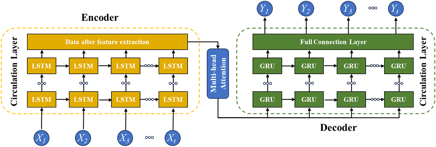
Figure 1: Framework of LSTM-GRU-multi-head attention

In the proposed model, the recurrent layer of the encoder employs LSTM. LSTM effectively captures long-term dependencies between time steps in temporal data modeling, making it particularly suitable for processing the sequential characteristics of sensor data. The recurrent layer of the decoder utilizes GRU, which has simpler structure. This design conserves computational resources while maintaining performance in generation tasks, thereby facilitating subsequent platform deployment. To enhance model performance, the proposed model incorporates a multi-head attention mechanism as a bridge for information transmission between the encoder and decoder. This ensures the model can focus on crucial time steps in the input sequence, thereby improving prediction accuracy.

2.3 Modules of LSTM-GRU-Multi-Head Attention

(1) Encoder Module

Encoders are used to extract features from time series data. The LSTM network employed in this study effectively captures long-term dependencies in extended sequences, enabling the extraction of rich feature representations from input sequences. The input to the encoder layer is the time series data Xenc=[x1ec,x2ec,⋯,xtec]. For each time step t, the LSTM unit updates its cell state Ct and hidden state ht based on the current input xtec and either the initial hidden state h0 or the previous hidden state ht−1. The core concept of this process is to regulate information flow through LSTM’s gating mechanism, enabling it to retain useful information while discarding unnecessary information. The recurrent layer structure of the encoder is illustrated in Fig. 2.

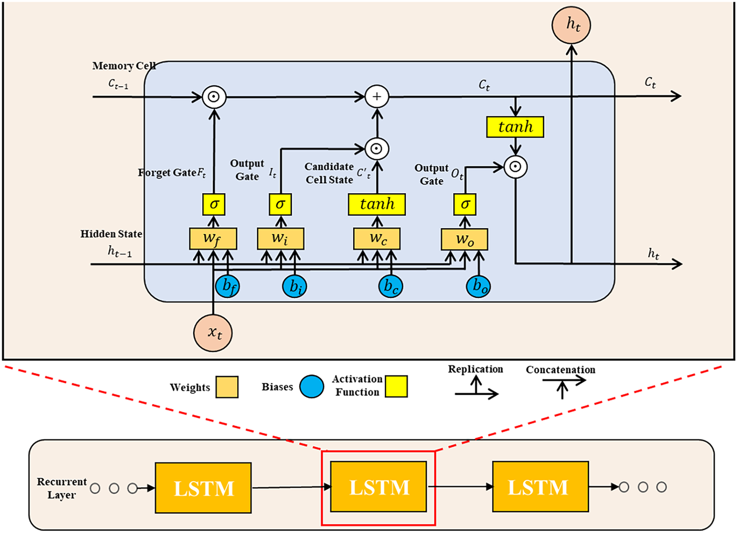
Figure 2: Encoder architecture diagram

LSTM primarily extracts features through gated recurrent units. Its key distinction from recurrent neural networks lies in its support for gating mechanisms in hidden states, enabling it to determine when to update or reset the hidden state.

It consists of three types of gate units: the input gate it, the forget gate ft, and the output gate ot. The input gate it determines how much of the current input is stored in the memory cell, the forget gate ft determines how much information from the memory cell of the previous time step is retained, and the output gate ot is used to generate the current hidden state ht. Additionally, a candidate memory cell ct~ is introduced. For the encoder input xtec, the computational processes of each gate unit are as shown in Eq. (2).

it=σ(Wi[ht−1,xtec]+bi)ft=σ(Wf[ht−1,xtec]+bf)ot=σ(Wo[ht−1,xtec]+bo)ct~=tanh(Wc[ht−1,xtec]+bc)(2)

where Wi,Wf,Wo,Wc are weight matrices, bi,bf,bo,bc are bias terms. These are all parameters to be learned in deep learning. The σ denotes the Sigmoid activation function, which ensures that the outputs of it,ft,ot range between 0 and 1. The tanh activation function is used to constrain the output range of ct~ to (−1, 1), facilitating subsequent computations.

The hidden layer output of the LSTM unit includes the hidden state and the memory cell. The memory cell ct is calculated from the input gate, forget gate, the memory cell of the previous time step, and the candidate memory cell. The hidden state htenc is ultimately obtained through the computation of the output gate and the memory cell, as shown in Eq. (3).

ct=ft⊙ct−1+it⊙ct~htenc=ot⊙tanh⁡(ct)(3)

The final encoder module outputs a hidden states sequence Henc=[h1enc,h2enc,⋯,htenc], where each hidden state htenccontains cumulative information from the first t time steps of the input sequence and incorporates both forward and backward contextual information. This provides essential temporal feature representations for the subsequent decoding process.

(2) Multi-Head Attention Module

The attention module is used to connect the encoder and decoder so that the decoder can dynamically attend to the encoder’s key information when generating each output, thereby improving model performance. Multi-head attention realizes parallel computation by projecting the inputs into multiple Query (Q), Key (K), and Value (V) spaces; each head computes an independent attention output, and the results of all heads are concatenated and passed through a linear layer to produce the final output. In the encoder–decoder architecture, the query vectors Q for attention come from the decoder’s hidden states, while the key vectors K and value vectors V come from the encoder outputs Henc. Suppose the decoder hidden state at the current time step is ht−1dec and the number of attention heads is h. For each head k ε {1,⋯,h}, the computations of the Q, K, and V vectors are given by Eq. (4).

Qk=WkQht−1decKk=WkKHencVk=WkVHenc(4)

where WkQ, WkK, and WkV are learnable parameter matrices. Common methods for computing attention scores include additive attention and dot-product attention; in this paper we employ dot-product attention to compute the attention scores. For the k-th attention head, the computation of the attention scores is given in Eq. (5).

headk=softmax(QkKkTdk)Vk(5)

QkKkT computes the inner product between the query matrix and the key matrix, yielding the attention scores. When input dimensions are large, computed scores may become excessively high. To prevent gradient instability, these scores are typically scaled. Typically, the attention scores are divided by a scaling factor, usually chosen as the square root of the dimension of the query and key matrices (dk). This aims to maintain a relatively small numerical range for the dot product, thereby stabilizing gradients. Next, the similarity scores between each query and all keys are normalized into a probability distribution via the softmax function. This step converts the attention scores of each query vector to all keys into weights, ensuring the sum of these weights equals 1. Finally, the computed attention weight matrix is multiplied by the value matrix V through matrix multiplication to obtain the final weighted sum result.

The above dot-product attention calculation occurs simultaneously across multiple attention heads. Inputs undergo parallel computation through these heads, each equipped with independent linear transformation matrices for queries, keys, and values. Each head independently computes its attention output, which is then concatenated to form a new matrix. To ensure the final output maintains the same dimension as the input, the concatenated matrix is multiplied by the linear transformation matrix Wo to achieve mapping. This yields the final output at of the multi-head attention mechanism. The computational process is illustrated in Eq. (6).

at=Concat(head1,head2,⋯,headk)W0(6)

at represents the intermediate vector obtained by weighting the hidden state output from the encoder through an attention mechanism, enabling the decoder to flexibly select features extracted from the encoder to generate the output at each time step.

(3) Decoder Module

The primary task of the decoder is to generate prediction results Y based on the encoder’s output at, which has been weighted by the attention mechanism. Its output method is incremental, meaning predictions for the next time step are generated based on the output of the previous time step. This approach captures dynamic changes and long-term dependencies in the data, flexibly handling various complex scenarios. However, as the sequence length increases, the computational complexity and number of parameters in the model may surge dramatically, limiting both training speed and inference speed. To address this issue, the decoder module employs GRU.

Compared to LSTM, GRU features a simpler structure. It regulates information flow solely through the update gate zt and reset gate rt, making it computationally more efficient with lower computational complexity than LSTM. The calculation processes for the zt (update gate), rt (reset gate), ht~ (candidate hidden state), and htdec (output hidden state) in GRU are shown in Eq. (7).

rt=σ(Wxrxtdc+Whr(ht−1dec⊕at))+br)zt=σ(Wxzxtdc+Whz(ht−1dec⊕at))+bz)h~t=tanh(Wxhxtdc+Whh(rt⊙(ht−1dec⊕at))+bh)htdec=(1−zt)⊙ht−1dec+zt⊙ht~(7)

where Wxr, Whr, Wxz, Whz, Wxh, Whh denote weight parameters, br, bz, bh denote bias parameters, σ represents the Sigmoid activation function, and tanh denotes the hyperbolic tangent activation function. ⊙ represents the Hadamard product, ⊕ represents vector merging, and xtdc denotes the input to the decoder. The output of the GRU is htdec at the current time step. This hidden state integrates both the current input information and the feature information from previous time steps. Finally, htdec is passed through a linear output layer to map it to the current prediction output yt, as shown in Eq. (8).

yt=Wouthtdec+bout(8)

where, Wout denotes the weight parameters of the output layer, and bout represents the weight matrix of the output layer. Due to the feedforward output mechanism, the current-time output serves as part of the next-time input, i.e., xt+1dc=yt. Ultimately, the decoder outputs Y=[y1,y2,⋯,yl], where l is the prediction stride.

2.4 Implementation of Multivariate Time Series Forecasting Model Based on LSTM-GRU and Multi-Head Attention

Multivariate time series forecasting can be divided into the following steps:

Step 1: Organize and consolidate data collected from multiple sensors of the electro-hydraulic servo material fatigue testing machine. Construct the dataset using the sliding window method and partition it into training and validation sets.

Step 2: Model construction and training. First, initialize model parameters. Input training data into the model, perform forward propagation through the encoder, multi-head attention, and decoder to obtain predicted values. Next, calculate the discrepancy between predicted and actual values using the loss function. Update model parameters via backward propagation based on the optimization algorithm, repeating this process until the loss ceases to decrease. Finally, the validation set data is input into the trained model to evaluate its performance, completing the model training. The pseudocode for the training process of the multivariate time series prediction model based on LSTM-GRU and Multi-head attention is shown in Algorithm 1.

Step 3: Deploy the trained multivariate time-series data prediction model for electro-hydraulic servo material fatigue testing machines in actual industrial settings. Use the actual sensor data collected as input for the prediction model to obtain forecast results, thereby completing the multivariate time-series data prediction process.

3  Case Study: Training and Evaluation of a Multivariate Time Series Prediction Model for an Electro-Hydraulic Servo Material Fatigue Testing Machine

3.1 Experimental Data Collection and Processing

Fig. 3 shows the SDZ3000 model testing machine produced by SinoTest. This article takes this type of testing machine as an example for research. The data for the multivariate time series prediction model of the electro-hydraulic servo material fatigue testing machine are obtained from sensors installed on its components. In total, seven sensors are involved, including four hydraulic pipe pressure sensors (100 Hz), one hydraulic pump motor power sensor (100 Hz), and two pipeline flow sensors (10 Hz). To facilitate data time-series alignment, flow parameters are resampled at 100 Hz. Since flow parameters do not exhibit abrupt changes in engineering applications, quadratic interpolation is employed for resampling. The seven sensors monitor key machine states—motor power, four-point pressures, and dual flows—all directly driven by the fatigue test load spectrum, frequency, and amplitude. The dataset covers >200 h of real tests across sinusoidal, random, and block loading (0.1–30 Hz).

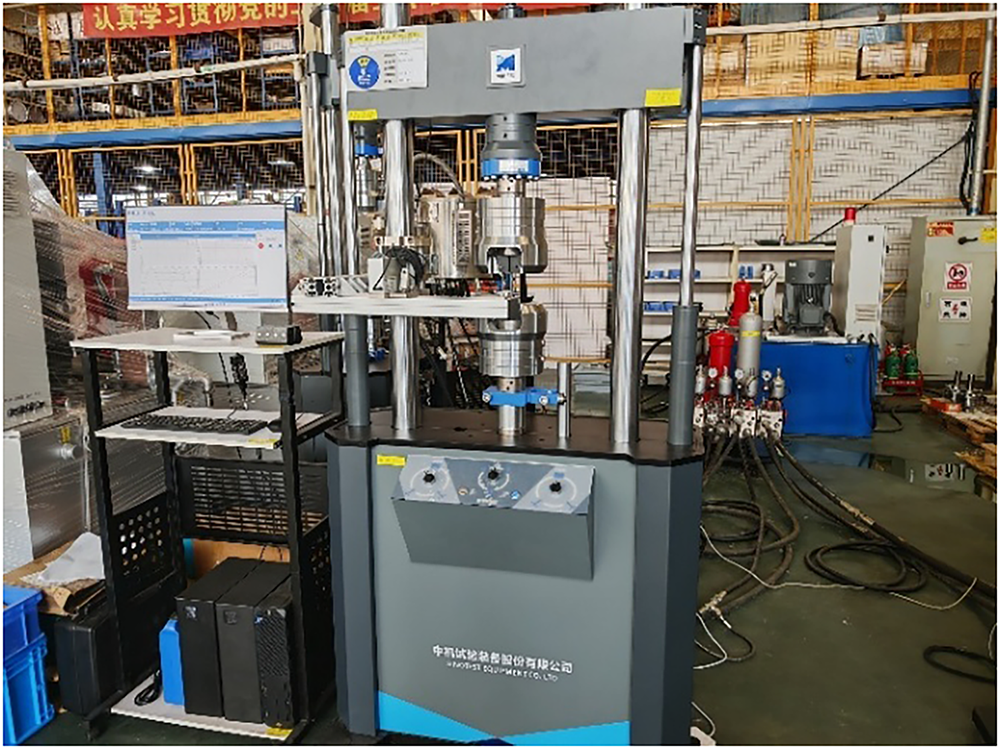
Figure 3: Experimental platform for multivariate time series prediction using an electro-hydraulic servo material fatigue testing machine

The multi-channel inputs—motor power, multi-point hydraulic pressures, and pipeline flow rates—are not independent but inherently coupled due to the underlying physics of the electro-hydraulic servo system. Specifically: Firstly, the flow rate in the pipeline is governed by the pressure differential across hydraulic components (e.g., servo valve, actuator) according to orifice flow laws, establishing a direct nonlinear relationship with multi-point pressures; Secondly, the motor power consumption of the hydraulic pump is primarily determined by the system pressure and flow demand, as per the hydraulic power equation P=p⋅Q/η (where p is pressure, Q is flow rate, and η is efficiency), implying that power dynamically responds to joint variations in pressure and flow; Thirdly, under cyclic loading conditions (e.g., sinusoidal or random spectra), pressure waves propagate through the pipeline, inducing time-delayed correlations among spatially distributed pressure sensors, while flow transients further modulate local pressure dynamics.

These well-established physical interactions confirm that the state variables exhibit strong, nonlinear, and time-varying cross-dependencies. Consequently, a predictive model must explicitly account for such multivariate couplings to achieve high fidelity. This motivates our integration of the multi-head attention mechanism, which adaptively learns the relevance of each input variable at every prediction step—thereby capturing both instantaneous relationships and delayed effects.

After acquiring the data, preprocessing is required to ensure that the data are suitable for model training. Prior to standardization and sliding-window segmentation, the raw multivariate time-series underwent quality control: all seven channels were synchronously sampled, ensuring consistent timestamps; isolated missing values (caused by occasional sensor dropouts) were filled by linear interpolation; high-frequency noise and sporadic spikes in pressure and flow signals—attributed to pump pulsation and valve dynamics—were mitigated using a zero-phase low-pass Butterworth filter (20 Hz cutoff), followed by outlier replacement for points exceeding ±4 standard deviations from the local median. This preprocessing preserves physical dynamics while ensuring data integrity for model training. Following preprocessing, standardization is performed to normalize all features to a common scale, thus avoiding undue dominance by any single feature during model training. Then, a sliding window method was adopted to partition the preprocessed data into the training set and validation set. The sliding window approach specifies a fixed window length L, which moves along the time axis step-by-step. In each movement, the window advances by S steps, thereby extracting multiple consecutive subsequences. Each subsequence serves as the model input X, while the data points immediately following the subsequence act as the corresponding prediction labels Y. Subsequently, 80% of the data were randomly selected as the training set and 20% as the validation set.

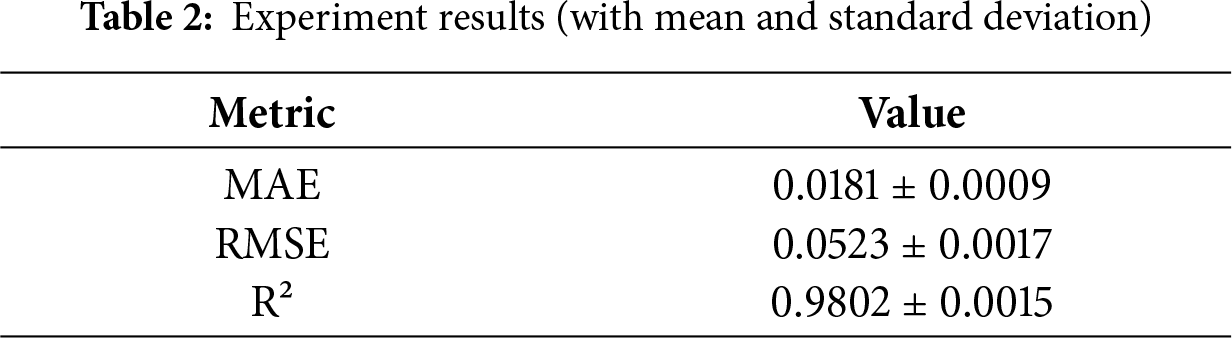
The evaluation of the proposed prediction model in this study focuses on prediction accuracy and the degree of model fit. In this paper, the Mean Absolute Error (MAE), the Root Mean Squared Error (RMSE), and the Coefficient of Determination (R2) are employed as the evaluation metrics.

3.2 Hyperparameter Tuning and Model Training of the Multivariate Time Series Prediction Model for the Electro-Hydraulic Servo Fatigue Testing Machine

Following the model construction process described earlier, it is necessary to determine the network architecture by setting the model hyperparameters. The hyperparameters involved in the model are as follows:

(1) Hidden layer dimension dh: This parameter refers to the number of neurons in each hidden layer. For both LSTM and GRU networks, the hidden layer dimension determines the capacity of each unit, thereby influencing the network’s ability to extract features.

(2) Number of multi-head attention heads h: This parameter controls the number of different perspectives from which the model can extract features at each time step, determining the number of parallel subspaces during attention computation.

(3) Time window size n and prediction length l: The time window size specifies how much historical data the model considers during each processing step. The prediction length indicates the number of future times steps the model predicts given the input sequence.

(4) Number of hidden layers N: This refers to the number of hidden layers in the LSTM and GRU within both the encoder and decoder. It governs the model’s depth and its ability to capture complex patterns in the data.

The hyperparameter settings for the model are shown in Table 1. The hardware configuration of the training environment is as follows: AMD Ryzen 2700X CPU, NVIDIA 2070 GPU, and 16 GB RAM.

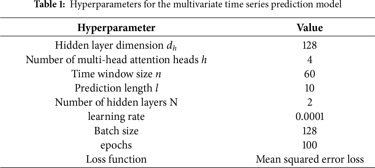
The hyperparameters were selected based on a combination of empirical trials and engineering considerations. Preliminary experiments showed that increasing the hidden dimension beyond 128 or attention heads beyond 4 yielded diminishing returns in validation accuracy relative to computational cost. Similarly, model depth beyond two layers did not significantly improve performance.

The loss during model training and the variation curves of related evaluation metrics are shown in Fig. 4. As the number of training iterations increases, the MSE loss on both the training and validation sets steadily declines, exhibiting a generally smooth downward trend.

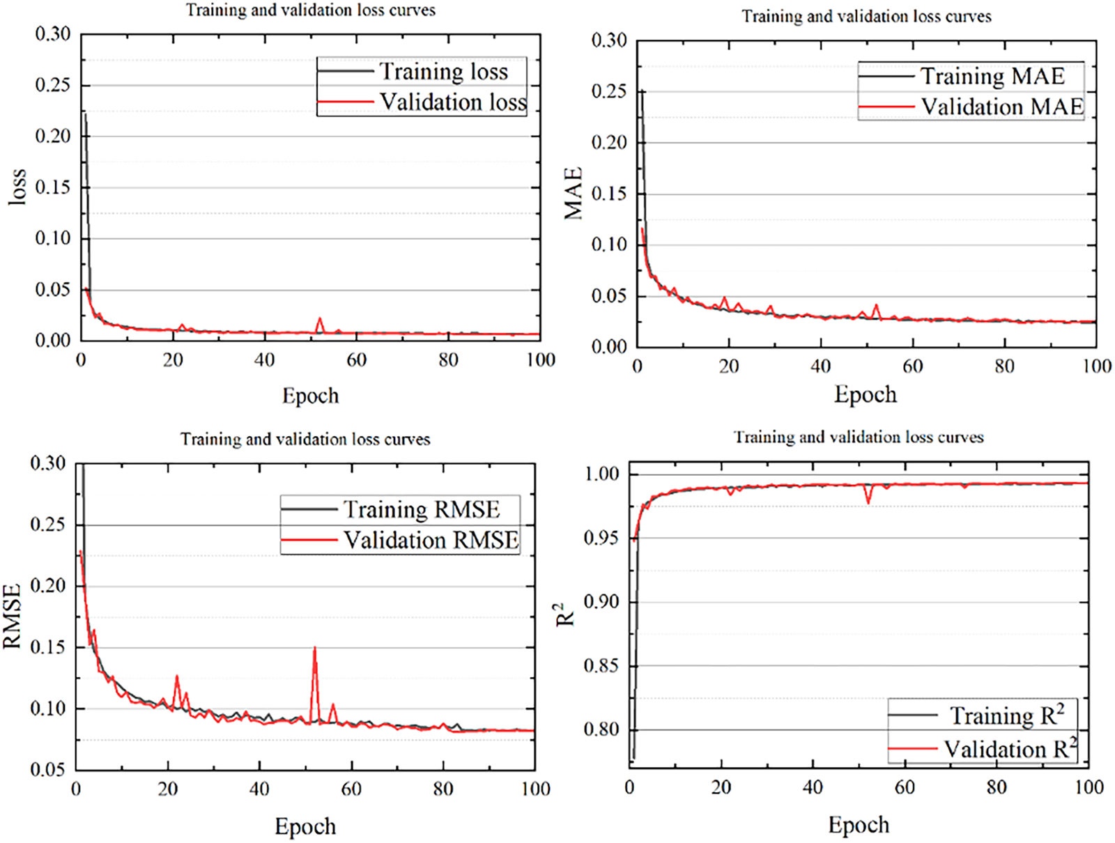
Figure 4: Loss curves and changes in evaluation metrics during model training

Eventually, the MSE loss on the validation set stabilizes below 0.01, indicating that the model gradually learns the temporal patterns in the data. Similarly, the MAE and RMSE values decrease with the increase in iteration count, ultimately stabilizing at approximately 0.018 and 0.052 on the validation set, respectively. This demonstrates that the errors between the predicted and actual values are relatively small, suggesting high prediction accuracy. Moreover, the R2 value increases over the course of training, stabilizing at approximately 0.98 on the validation set, indicating that the model achieves a high degree of fit to the data. These results demonstrate that the proposed multivariate time series prediction model for the electro-hydraulic servo fatigue testing machine can effectively capture the characteristics of time-series data and deliver accurate predictions. The above experimental results were accomplished through ten random experiments. Table 2 reports the mean and standard deviation of each index after the experiments.

After verifying that the model performs well on both the training and validation sets, this paper further examines its performance in practical applications. Using pipeline flow rate, motor power, and system pressure as model inputs, the trained model generates corresponding predicted values. To better visualize the local prediction performance, a 600-s segment of data is extracted, and the predicted values are plotted against the actual values, as shown in Fig. 5.

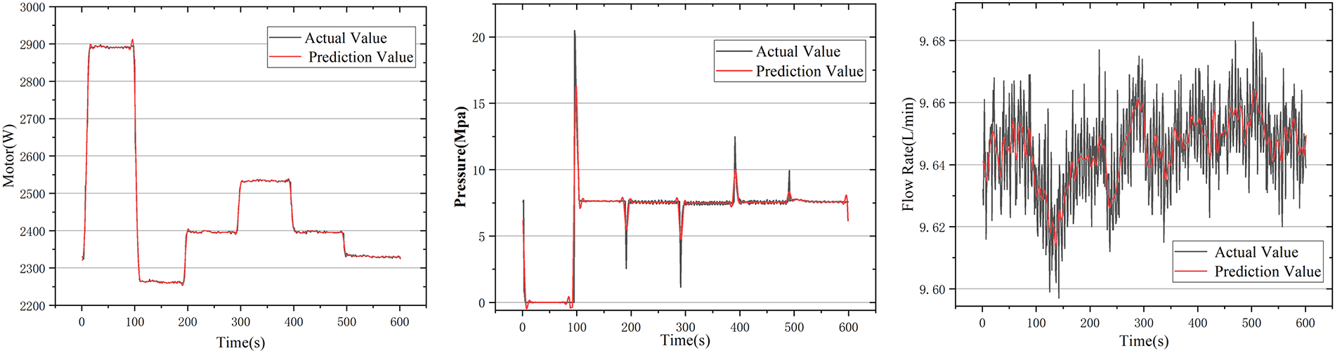
Figure 5: Comparison between predicted and actual time series for representative variables. All three outputs—and the remaining four sensor channels—are predicted simultaneously from the same 7-dimensional input sequence, which explicitly models cross-variable dependencies

From the comparison in Fig. 5, it is evident that the trend of the predicted data closely follows that of the actual data. The model is able to capture the dynamic variations in the data with only minimal error. These results indicate that the model maintains excellent predictive capability and robustness in practical application scenarios.

4  Discussion

4.1 Sensitivity Analysis of Prediction Horizon l

The prediction horizon is a critical hyperparameter in a multivariate time series forecasting model, as it determines the range of future time steps the model can predict. A longer prediction horizon allows the model to foresee further into the future, which is beneficial for early detection of potential faults and anomalies. However, prediction errors may accumulate as the horizon increases. Moreover, a longer horizon inevitably demands more computational resources. Therefore, it is essential to determine the optimal prediction horizon l through experiments, achieving a balance between predictive performance and computational cost. With the time window length fixed at 60, the model’s performance on the validation set was compared under different prediction horizons in terms of MSE loss, MAE, RMSE, and training time. The experimental results are shown in Fig. 6 and Table 3.

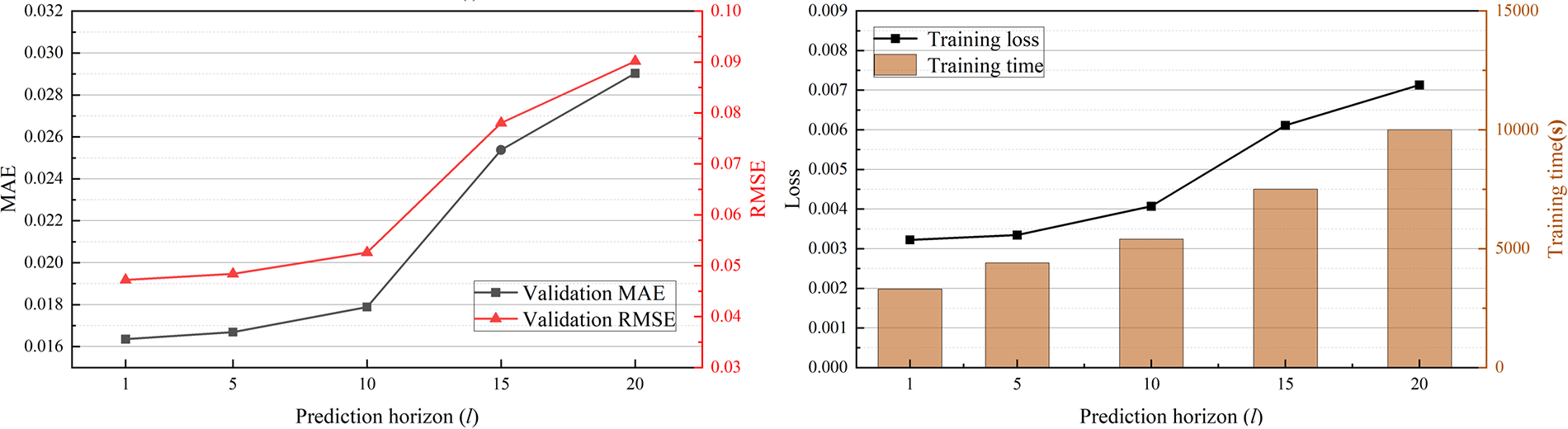
Figure 6: Sensitivity analysis of prediction step size

From the experimental results, it can be observed that when the prediction horizon is 1, 5, or 10, the model’s MSE loss, MAE, and RMSE remain at low levels, while computational cost increases gradually with l. However, when l increases to 15, the model’s loss, error, and computational demand increase significantly. Compared with l=10, the MSE loss rises by approximately 50%, and MAE, RMSE, as well as computational cost increase by roughly 40%. Therefore, selecting l=10 achieves a good balance between prediction accuracy and computation efficiency.

It should be noted that while l = 1 and l = 5 achieve slightly lower prediction errors, their very short horizons offer limited practical value for prognostic health monitoring or early anomaly detection. In contrast, l = 10 strikes a favorable balance: it provides a meaningful prediction window for residual-driven diagnostics while maintaining high accuracy (MAE ≈ 0.018) and reasonable computational overhead. Thus, the selection of l = 10 is motivated by deployment-oriented considerations rather than metric minimization alone.

4.2 Ablation Studies

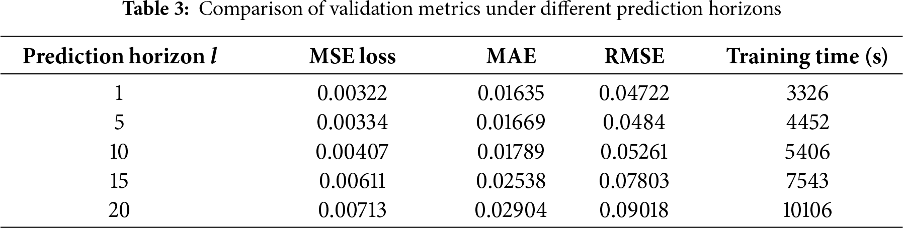
To verify the effectiveness of encoder, decoder, and MHA mechanism in the proposed multivariate time series forecasting model, three sets of ablation experiments were designed. An ablation experiment involves progressively removing or replacing key components of the model to evaluate their contribution to the overall performance. The network configurations are given in Table 4.

The experiments include: A: Proposed model; B: Replacing multi-head attention with single-head attention; C: Removing the decoder; D: Removing the attention mechanism.

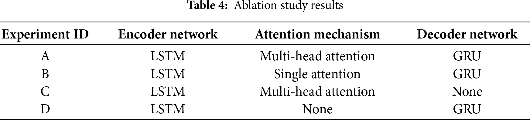
All four models were trained using the same parameters and dataset as in above section. The evaluation results on the validation set are presented in Fig. 7 and Table 5.

Figure 7: Comparison of ablation study

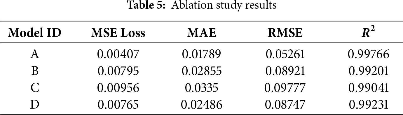
The results indicate that both the decoder module and the attention mechanism contribute to improving the prediction accuracy. Specifically, applying multi-head attention yields better performance than single-head attention. Overall, for an architecture using only an encoder and an attention mechanism, adding a decoder or replacing single-head attention with multi-head attention reduces the MSE loss by approximately 17% and decreases the MAE and RMSE by about 26%. When both the decoder and multi-head attention are applied simultaneously, all four evaluation metrics achieve their best values. Therefore, the ablation experiments confirm that incorporating both the decoder and multi-head attention into the proposed architecture significantly enhances prediction performance.

4.3 Method Comparison

To further demonstrate the effectiveness of the method proposed in this paper, this paper compares other types of methods. Among the data-driven methods, we compare the widely used Transformer method in classical system identification approaches. We compared the NARX and Hammerstein-Wiener methods. All models are implemented using the same training/validation segmentation, the same input variables, and the same prediction range (l = 10). The hyperparameters of each baseline model are adjusted through grid search on the validation set to ensure fair comparison. The comparison results are shown in Table 6.

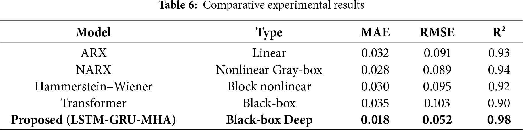
The results show that although traditional models achieved moderate performance (for example, NARX: RMSE ≈ 0.089, R² ≈ 0.94), the model we proposed consistently outperformed them by a significant margin. This indicates that the proposed architecture can better capture the complex spatio-temporal coupling and nonlinear dynamic characteristics existing in real fatigue testing machines. Beyond quantitative metrics, we further examine the model’s behavior to enhance interpretability. First, the dataset covers diverse fatigue testing scenarios (multiple load spectra), and consistent R² > 0.97 across them confirms good generalization. Second, prediction errors are slightly elevated for flow rates during abrupt load changes—reflecting inherent hydraulic lag—yet remain bounded (MAE < 0.02). Third, attention weight analysis shows the model preferentially attends to upstream pressure channels when forecasting flow, and to motor power for long-term pressure trends, consistent with fluid power principles. This suggests the attention mechanism captures causal physical relationships, making it not just a performance booster but also a potential tool for system diagnostics.

4.4 Potential and Technical Challenges

While this study focuses on open-loop prediction for health monitoring, an immediate extension is to close the loop by integrating the predictor with the machine’s feedback control system. For instance, predicted residuals between actual and expected system responses could be used to adjust PID setpoints or trigger adaptive gain scheduling, enabling proactive compensation before large deviations occur. Although challenges remain—including real-time inference speed, model trustworthiness under unseen conditions, and rigorous stability guarantees—such predictive-control fusion represents a promising path toward autonomous, self-aware fatigue testing platforms.

4.5 Deployability

To validate the claim of near-real-time deployability, we measured the inference performance of the trained model on representative hardware. Using the same test platform (AMD Ryzen 7 2700X CPU, NVIDIA RTX 2070 GPU, 16 GB RAM), the model processes a single prediction step (forecasting 10 future time steps from a 60-step input window) in 8.3 ms on GPU and 24.6 ms on CPU. The computational cost per prediction is approximately 1.2 GFLOPs, and the model occupies ~42 MB of memory (including weights and intermediate activations). Given that the sampling interval of the sensor data is 10 ms (100 Hz), GPU-based inference satisfies real-time requirements (latency < sampling period), while CPU execution enables deployment in resource-constrained edge environments with slight buffering. These results confirm the practical feasibility of integrating the model into on-line monitoring systems for electro-hydraulic fatigue testers.

5  Conclusion

This study addresses the strongly coupled, nonlinear, time-varying, multivariate characteristics of electro-hydraulic servo material fatigue testing machines, and proposes a sequence-to-sequence multivariate time series prediction model that integrates an LSTM-based encoder, a GRU-based decoder, and a multi-head attention mechanism. The model leverages multi-channel inputs and cross-variable information interaction, capturing both short-term, high-frequency dynamics and long-term, slow drift effects. On real bench test data, the model achieves high prediction accuracy and stability—with the MSE on the validation set stabilizing below 0.01, MAE and RMSE at approximately 0.018 and 0.052, respectively, and the coefficient of determination R2 around 0.98. Comparative and ablation experiments demonstrate a significant advantage over traditional system identification approaches and single RNN architectures, confirming the importance of the decoder and multi-head attention in capturing cross-variable coupling and key temporal steps. Sensitivity analysis indicates that a prediction horizon of l=10 offers an optimal balance between accuracy and computational cost, making near-real-time deployment feasible.

In summary, the proposed multivariate time series prediction framework achieves a balanced performance in prediction accuracy, robustness, and engineering applicability. It provides a practical, data-driven pathway for high-precision control, health management, and test credibility evaluation in electro-hydraulic servo material fatigue testing equipment, offering tangible benefits for enhancing operational reliability and reducing life-cycle costs.

Acknowledgement: Not applicable.

Funding Statement: This work was supported by Natural Science Foundation of China (NSFC), Grant number 5247052693.

Author Contributions: The authors confirm contribution to the paper as follows: study conception and design: Guotai Huang; data collection: Xiyu Gao; analysis and interpretation of results: Peng Liu; draft manuscript preparation: Liming Zhou. All authors reviewed the results and approved the final version of the manuscript.

Availability of Data and Materials: Data not available due to legal restrictions.

Ethics Approval: Not applicable.

Conflicts of Interest: The authors declare that they have no known competing financial interests or personal relationships that could have appeared to influence the work reported in this paper.

References

1. Lin H, Liu W, Zhang D, Chen B, Zhang X. Study on the degradation mechanism of mechanical properties of red sandstone under static and dynamic loading after different high temperatures. Sci Rep. 2025;15(1):11611. doi:10.1038/s41598-025-93969-4. [Google Scholar] [PubMed] [CrossRef]

2. Sun C, Li J, Tan Y, Duan Z. Proposed feedback-linearized integral sliding mode control for an electro-hydraulic servo material testing machine. Machines. 2024;12(3):164. doi:10.3390/machines12030164. [Google Scholar] [CrossRef]

3. Niu S, Wang J, Zhao J, Shen W. Neural network-based finite-time command-filtered adaptive backstepping control of electro-hydraulic servo system with a three-stage valve. ISA Trans. 2024;144:419–35. doi:10.1016/j.isatra.2023.10.017. [Google Scholar] [PubMed] [CrossRef]

4. Goutier M, Vietor T. Parametric study of geometry and process parameter influences on additively manufactured piezoresistive sensors under cyclic loading. Polymers. 2025;17(12):1625. doi:10.3390/polym17121625. [Google Scholar] [PubMed] [CrossRef]

5. Jia W, Song W, Chen H, Li S. Advancements in electrohydraulic fatigue testing: innovations in variable resonance frequency control and comprehensive characterization. Mech Syst Signal Process. 2025;224:111999. doi:10.1016/j.ymssp.2024.111999. [Google Scholar] [CrossRef]

6. Tsay RS. Testing and modeling multivariate threshold models. J Am Stat Assoc. 1998;93(443):1188–202. doi:10.1080/01621459.1998.10473779. [Google Scholar] [CrossRef]

7. Li Y, Zhang H, Wen L, Shi N. A prediction model for deformation behavior of concrete face rockfill dams based on the threshold regression method. Arab J Sci Eng. 2021;46(6):5801–16. doi:10.1007/s13369-020-05285-w. [Google Scholar] [CrossRef]

8. Neu DA, Lahann J, Fettke P. A systematic literature review on state-of-the-art deep learning methods for process prediction. Artif Intell Rev. 2022;55(2):801–27. doi:10.1007/s10462-021-09960-8. [Google Scholar] [CrossRef]

9. Zhang M, Yuan ZM, Dai SS, Chen ML, Incecik A. LSTM RNN-based excitation force prediction for the real-time control of wave energy converters. Ocean Eng. 2024;306:118023. doi:10.1016/j.oceaneng.2024.118023. [Google Scholar] [CrossRef]

10. Golshanrad P, Faghih F. DeepCover: advancing RNN test coverage and online error prediction using state machine extraction. J Syst Softw. 2024;211:111987. doi:10.1016/j.jss.2024.111987. [Google Scholar] [CrossRef]

11. Olu-Ajayi R, Alaka H, Sulaimon I, Sunmola F, Ajayi S. Building energy consumption prediction for residential buildings using deep learning and other machine learning techniques. J Build Eng. 2022;45:103406. doi:10.1016/j.jobe.2021.103406. [Google Scholar] [CrossRef]

12. Fantini DG, Silva RN, Siqueira MBB, Pinto MSS, Guimarães M, Brasil ACP. Wind speed short-term prediction using recurrent neural network GRU model and stationary wavelet transform GRU hybrid model. Energy Convers Manag. 2024;308:118333. doi:10.1016/j.enconman.2024.118333. [Google Scholar] [CrossRef]

13. Tian Q, Luo W, Guo L. Water quality prediction in the Yellow River source area based on the DeepTCN-GRU model. J Water Process Eng. 2024;59:105052. doi:10.1016/j.jwpe.2024.105052. [Google Scholar] [CrossRef]

14. Sayah M, Guebli D, Al Masry Z, Zerhouni N. Robustness testing framework for RUL prediction Deep LSTM networks. ISA Trans. 2021;113:28–38. doi:10.1016/j.isatra.2020.07.003. [Google Scholar] [PubMed] [CrossRef]

15. Shahid F, Zameer A, Muneeb M. Predictions for COVID-19 with deep learning models of LSTM, GRU and Bi-LSTM. Chaos Solitons Fractals. 2020;140:110212. doi:10.1016/j.chaos.2020.110212. [Google Scholar] [PubMed] [CrossRef]

16. Xiang S, Qin Y, Zhu C, Wang Y, Chen H. LSTM networks based on attention ordered neurons for gear remaining life prediction. ISA Trans. 2020;106(1):343–54. doi:10.1016/j.isatra.2020.06.023. [Google Scholar] [PubMed] [CrossRef]

17. Han Y, Qi W, Ding N, Geng Z. Short-time wavelet entropy integrating improved LSTM for fault diagnosis of modular multilevel converter. IEEE Trans Cybern. 2022;52(8):7504–12. doi:10.1109/TCYB.2020.3041850. [Google Scholar] [PubMed] [CrossRef]

18. Huang T, Zhang Q, Tang X, Zhao S, Lu X. A novel fault diagnosis method based on CNN and LSTM and its application in fault diagnosis for complex systems. Artif Intell Rev. 2022;55(2):1289–315. doi:10.1007/s10462-021-09993-z. [Google Scholar] [CrossRef]

19. Wang S, Shi J, Yang W, Yin Q. High and low frequency wind power prediction based on Transformer and BiGRU-Attention. Energy. 2024;288:129753. doi:10.1016/j.energy.2023.129753. [Google Scholar] [CrossRef]

20. Yuan X, Huang L, Ye L, Wang Y, Wang K, Yang C, et al. Quality prediction modeling for industrial processes using multiscale attention-based convolutional neural network. IEEE Trans Cybern. 2024;54(5):2696–707. doi:10.1109/tcyb.2024.3365068. [Google Scholar] [PubMed] [CrossRef]