Two-Scale Concurrent Topology Optimization Method Based on Boundary Connection Layer Microstructure

1  Introduction

Porous structures composed of multiple lattice unit cells are widely used in engineering due to their high strength-to-weight and stiffness-to-weight ratios, as well as excellent thermal insulation, vibration damping, and energy absorption [1–3]. However, designing microstructures and their macroscopic layouts to meet specific performance goals remains a key challenge. Unlike size and shape optimization, topology optimization effectively explores material distribution by automatically finding optimal layouts under given loads and boundary conditions, often producing innovative, counter-intuitive designs. Over recent decades, it has advanced significantly, yielding major methods such as the SIMP method [4], the level set method [5–8], the evolutionary structural optimization (ESO) method [9–11], the moving morphable components/voids (MMC/MMV) method [12–14], and composite approaches [15].

Since Bendsøe and Kikuchi [16] introduced the homogenization method in 1988, topology optimization has been used for two-scale material design. Within a macrostructure, different regions serve different mechanical functions, so each should have a tailored microstructure to maximize multiscale performance. Rodrigues et al. [17] first developed a method to optimize both macroscopic and microscopic layouts simultaneously. Xia and Breitkopf [18] later extended it to nonlinear problems. However, designing microstructures point by point leads to high computational costs and poor connectivity between cells. To address this, researchers have proposed improved approaches. For instance, Wang et al. [19] created graded microstructures using local level-cutting of the signed distance function. Zong et al. [20] improved connectivity with a global cutting equation. Li et al. [21] designed uniform microstructures with tunable aspect ratios for flexible combinations. Another approach divides the domain into subdomains, each with a different microstructure. These include manual partitions [22], density-based schemes [23], and stress orientation-based methods [24]. Although these methods achieve an effective balance between computational cost and design space, they still inadequately address material behavior and interface connectivity in the boundary regions of microstructures. These important issues are worthy of further study by researchers. In this paper, we mainly focus on the connection reliability between microstructures.

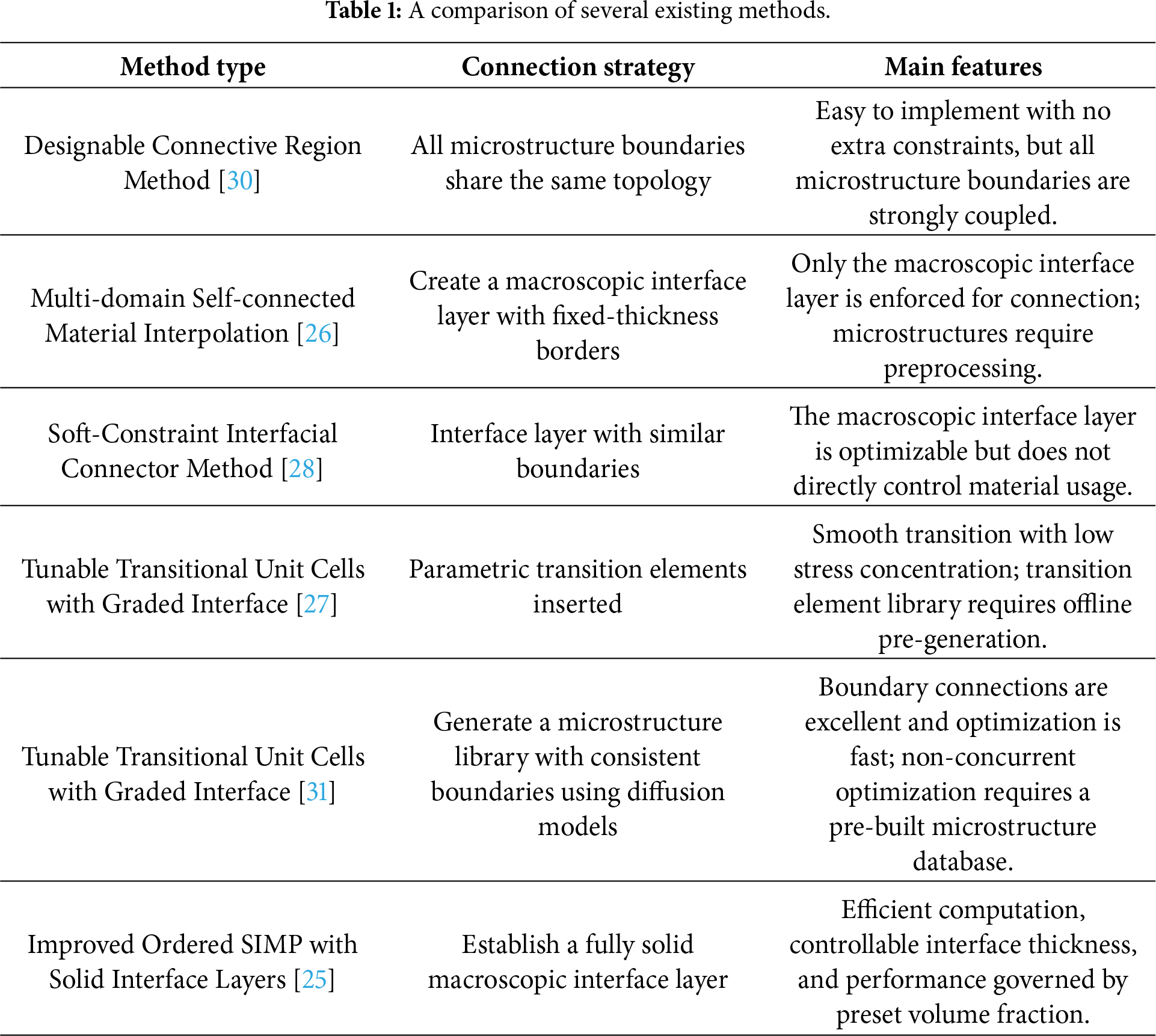
In recent years, the issue of microstructure connectivity has increasingly drawn attention in the manufacturing process using 3D printing technology. Gu et al. [25] proposed a multi-scale concurrent optimization method that enables simultaneous design of macroscopic and microscopic structures in periodic multi-microstructure systems with solid interfaces. Luo et al. [26] developed a “self-connecting material interpolation model” to enforce material continuity in transition zones, which effectively reducing topological discontinuities across distinct microstructures. Wei et al. [27] embedded graded transitional unit cells between base microstructures, achieving smooth transitions in material properties and geometry while preserving interfacial structural integrity. Gu et al. [28] introduced a “connective microstructure” approach that employs specialized connecting units geometrically matched to lattice boundaries, thereby enhancing connectivity in multi-lattice architectures. Hu et al. [29] established a two-scale concurrent optimization framework for polycrystalline lattices under explicit physical connectivity constraints, integrating microstructural topology, macroscopic material distribution, and global layout. Liu et al. [30] achieved robust connections between heterogeneous microstructures by predefining connection regions and maintaining their topological consistency throughout optimization. Feng et al. [31] leveraged a guided diffusion model to generate a comprehensive set of boundary-consistent microstructures with tunable elastic moduli, simultaneously addressing connectivity and computational efficiency. Liu et al. [32] ensured microstructural connectivity in variable-density designs by fixing a thin material layer at each microstructure boundary. We have summarized several existing methods, as shown in Table 1. In conclusion, most existing studies have focused on addressing connection issues between different types of microstructures, while research on the reliability of connections among identical microstructures remains relatively limited. Therefore, developing a method that is highly versatile, easily implementable, and capable of effectively improving connection reliability for both identical and heterogeneous microstructures continue to hold significant research value and practical significance.

This paper proposes a two-scale concurrent topology optimization method with a boundary connection layer. By parametrically constructing a boundary connection layer with a fixed geometry, the contact area between adjacent microstructures is increased, thereby enhancing the reliability of the connection between adjacent microstructures. Meanwhile, only the material layout in the internal free design domain is freely evolved. This method reduces computational costs while balancing performance and connection reliability, and is easy to implement. The remainder of this paper is arranged as follows: Section 2 presents the design principles of the connectable microstructure. Section 3 provides the numerical implementation scheme. Section 4 presents the problem formulation and sensitivity analysis. Sections 5 and 6 respectively provide numerical examples and conclusions.

2  Design Principles of Microstructure with Boundary Connection Layer

2.1 Analysis of Connectivity Problems

In the two-scale topology optimization framework grounded in homogenization theory, the material within each macroscopic finite element is treated as an equivalent homogeneous medium. Under this assumption, macroscopic elements remain fully connected (as shown in Fig. 1), exhibiting high interfacial strength, and the resulting optimal macrostructure inherently relies on this idealized continuity.

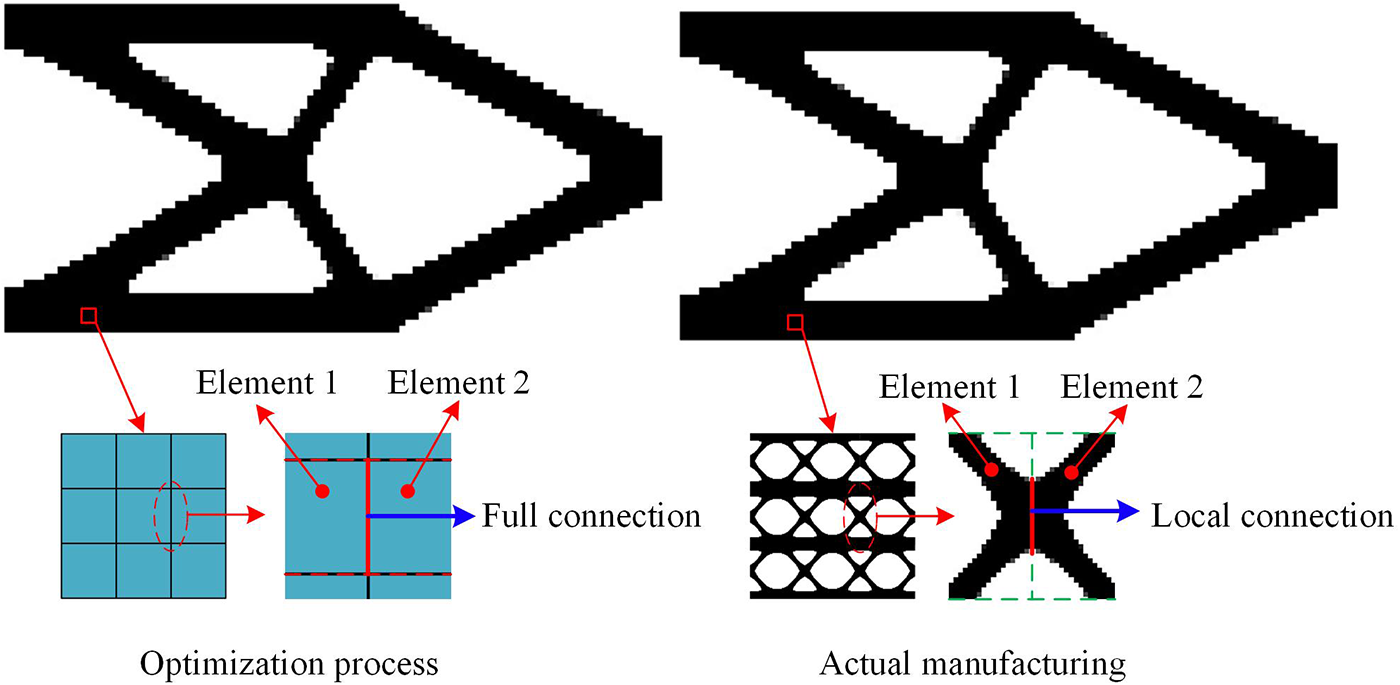
Figure 1: The connection strength between microstructures.

It should be emphasized that the microstructure influences macro-scale optimization solely through its equivalent mechanical properties, while its actual geometry, particularly material distribution and boundary connectivity within the unit cell, is not explicitly modeled. Although this approach enhances computational efficiency and satisfies numerical requirements, it neglects microstructural connectivity, leading to significant drawbacks. Poor connectivity results in discontinuous load paths and stress concentrations, thereby reducing structural stiffness, strength, and fatigue life. From a manufacturing standpoint, weak or isolated regions are prone to defects such as incomplete fusion, warpage, or interlayer cracking [28]. From a numerical standpoint, violating the periodicity assumption distorts predictions of equivalent properties and may induce numerical instability or false convergence during optimization. These connectivity-related limitations represent critical barriers to the practical manufacturability of optimized designs.

Current research on connectivity issues primarily focuses on the transition treatment between different microstructures (as shown in Fig. 2). A common approach involves identifying microstructural boundaries by computing the gradient of the macroscopic relative density distribution and introducing a dedicated transitional microstructure. However, this type of method has several limitations:

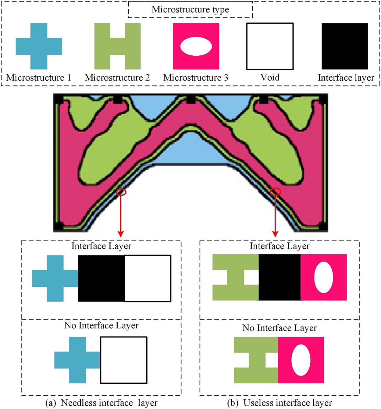
Figure 2: Classification of ineffective interface layer [32].

(1)   As illustrated in Fig. 2b, the two microstructures are well connected without connectivity issues. However, an interface layer still forms due to the density gradient, even though it is unnecessary.

(2)   This type of method will also introduce interface layer between the microstructure and the void regions (as shown in Fig. 2a) where interface layers are applied to the microstructure and the void phase), while such interface layers are not required in the actual structure.

(3)   It is unable to effectively solve the problem of insufficient connection strength between the same type of microstructures.

(4)   When the number of microstructure types is large, the number of interface layers increases sharply, complicating the problem.

The essence of connectivity issues lies in the interface characteristics between adjacent microstructures. Therefore, the approach of enhancing connectivity merely by improving one of the microstructures often has limitations. For this reason, this paper proposes a new method based on enhancing the connectivity of the microstructure itself: by introducing a controllable connection layer at the microstructure boundary (as shown in Fig. 3), thereby improving its inherent connection ability. This method not only applies to improving the connectivity between different microstructures, but also enhances the connection performance among the same microstructures, fundamentally increasing the connection reliability of the microstructure units themselves. It thus offers a pathway for achieving high-performance and highly manufacturable two-scale topology-optimized structures.

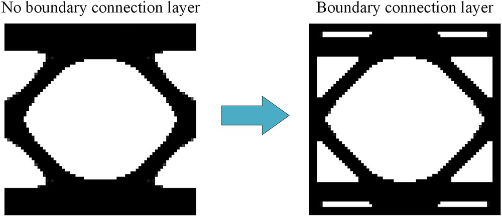
Figure 3: Microstructure with boundary connection layer.

2.2 Structural Characteristics and Design Strategies of Microstructure with Boundary Connection Layer

This paper introduces a design strategy of establishing a connection layer at the boundary of microstructures to enhance their self-connection ability. Taking the common two-dimensional square microstructure design domain as an example, the structural characteristics and design strategy will be elaborated in detail.

2.2.1 Structural Characteristics of Microstructure with Boundary Connection Layer

First, the microstructural design domain Ωm, which is composed of a single material, is partitioned into two functional regions. The free design domain is Ωm1 and the boundary connection region is Ωm2, respectively, where:

Ωm2∪Ωm1=Ωm(1)

The relationship among the three is shown in Fig. 4.

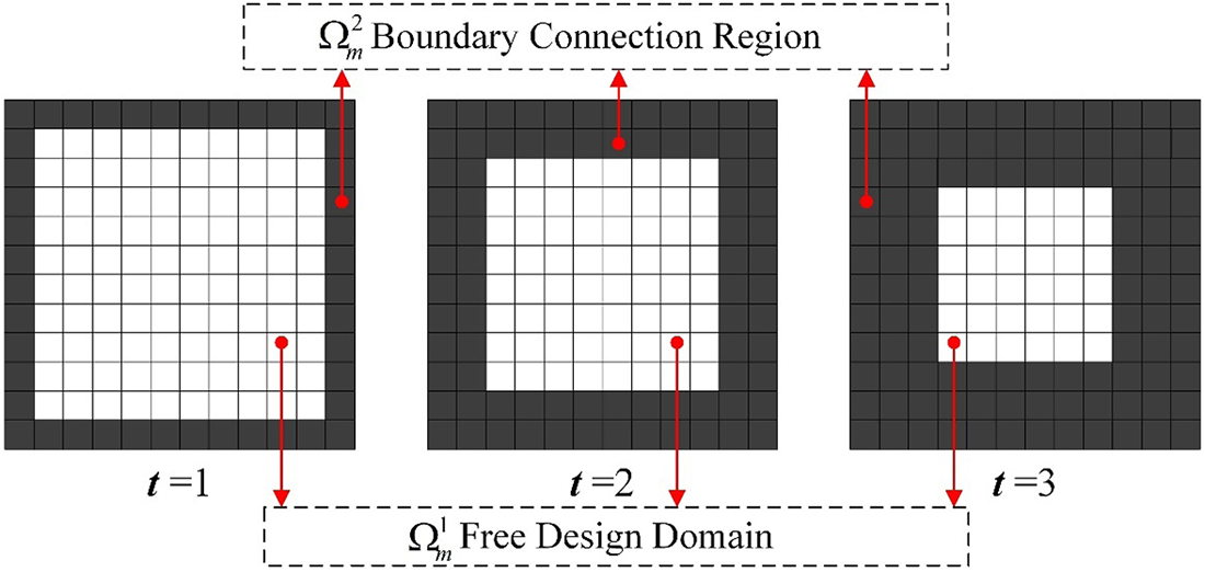
Figure 4: Microstructure with controllable boundary connection layer.

a.   Boundary Connection Region:

The elements within the Ωm2 region are forcibly assigned materials at the initial stage and do not participate in variable updates throughout the optimization process. Therefore, there is no need to calculate their sensitivity information, which reduces the computational cost to a certain extent. Upon completion of the optimization iteration, a uniform and dense connection layer is consistently formed around the microstructure, ensuring reliable interfacial performance in macroscopic assembly. Furthermore, the thickness of connection layer is explicitly controlled by the parameter t (as shown in Fig. 4), allowing designers to flexibly tailor the extent of boundary reinforcement and achieve precise alignment between microstructural performance and macroscopic assembly requirements.

b.   Free Design Domain:

The elements within the Ωm1 region are taken as the core design objects for optimization. Through multiple rounds of iterative updates, this region can autonomously adjust the material distribution, enabling the microstructure to achieve the optimal topological configuration for lightweight, high stiffness or specific functional orientation while meeting the overall mechanical performance requirements of the macrostructure.

The two functional regions jointly define a complete microstructure design domain: the boundary connection region Ωm2 ensures reliable interfacial connection, while the free design domain Ωm1 enables mechanical performance optimization. This approach allows the final microstructure to simultaneously satisfy macroscopic mechanical requirements and maintain robust assembly connectivity.

2.2.2 Design Strategies with Microstructures of Boundary Connection Layer

Take the common 2D square microstructure design domain as an example for illustration. By using the finite element method, the square design domain Ωm is discretized into Nm×Nm four-node rectangular elements. The upper limit of the overall material volume of the microstructure is stipulated as Vm0. As shown in Fig. 5, the schematic illustrates the design of the connectable microstructure and clearly outlines its implementation process.

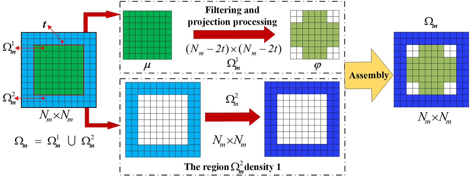
Figure 5: Boundary connection layer application strategy.

(1)   First, the Nm×Nm microstructure design domain is divided into a boundary connection region and a free design domain. The connection region is designated for generating a connection layer, the thickness of which is controlled by the parameter t, while the dimension of the boundary connection region is Nm×Nm.

(2)   For the finite elements within the free design domain Ωm1, the SIMP method is employed to enable free evolution toward an optimal topological configuration. Density filters combined with exponential Heaviside projection are applied to eliminate numerical instabilities such as checkerboard patterns and gray-scale elements.

(3)   The finite elements within the boundary connection region Ωm2 are forcibly assigned material without undergoing variable updates, and their material volume fraction is explicitly prescribed as:

Vt=(Nm−t)×4×t/Nm2,Nm,t∈N and t<Nm2(2)

where Vt represents the volume fraction of the material occupied by the boundary connection layer in the microstructure, t denotes the thickness of the boundary connection layer. Nm is the mesh resolution in each spatial direction.

(4)   Since the boundary connection region occupies a fixed amount of material, the upper limit of the material volume fraction in the free design domain Ωm1 is defined as:

Vm=Vm0−Vt(3)

here, Vm denotes the volume fraction of the free design domain and Vm0 is the maximum allowed volume fraction in the microstructure.

(5)   Combine the two functional regions and use the homogenization method to solve for the equivalent elastic matrix of the microstructure. Then, based on SIMP, build the material model, carry out FEA at the macrostructure and calculate the objective function and constraints.

(6)   Calculate the macro and micro sensitivities and update the variables using the Optimality Criteria (OC) method. Then, evaluate whether the convergence criteria are satisfied.

(7)   Repeat until the compliance of the macrostructure and all volume constraints are stably convergent. The optimization flowchart is shown in Fig. 6.

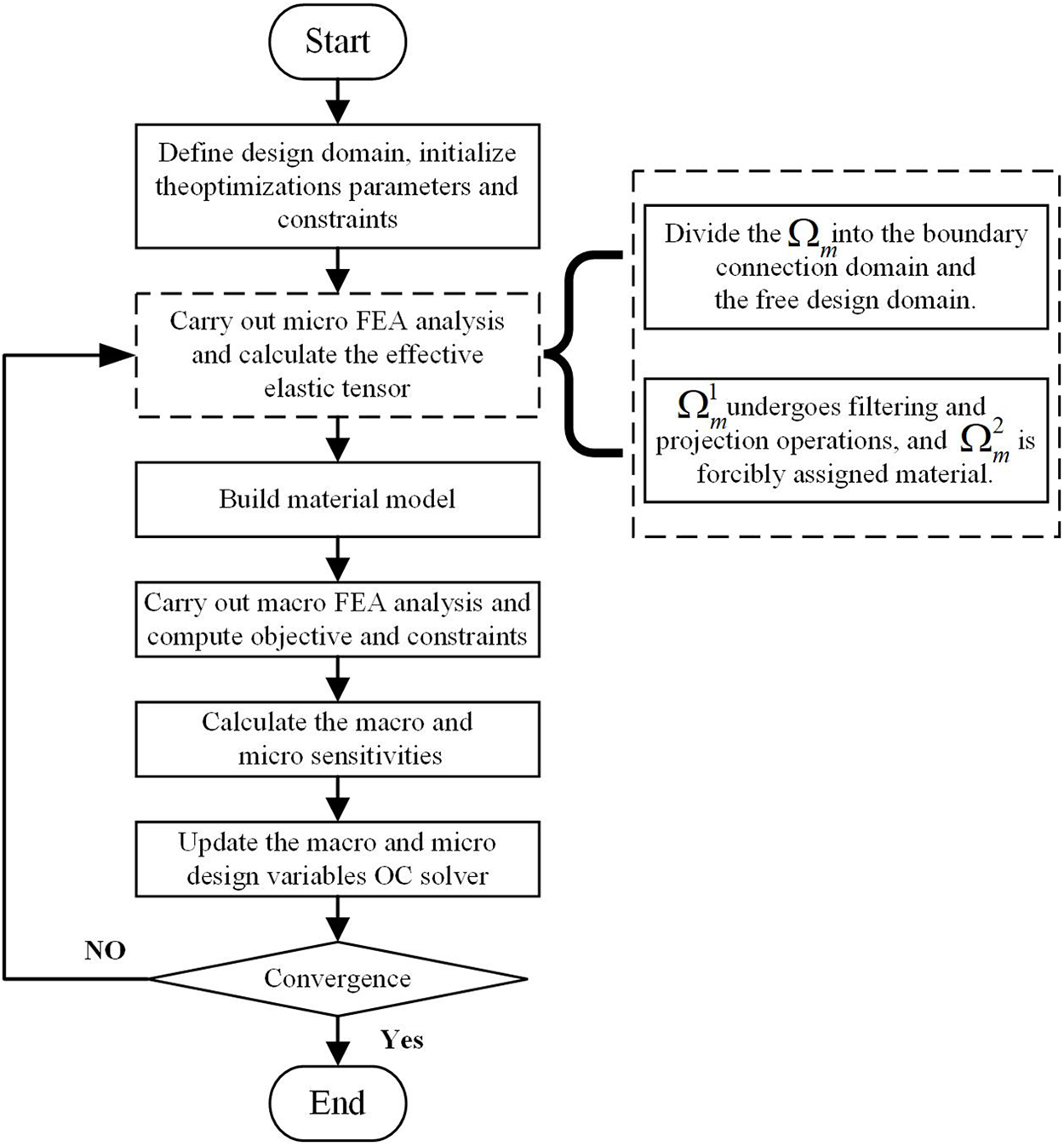
Figure 6: Flowchart of two-scale concurrent topology optimization.

3  Numerical Implementation

3.1 Two-Scale Topology Optimization Interpolation Model

The macroscopic structure is composed of periodic microscopic structures and can be regarded as a homogeneous material at the macroscale. The micro-design variable ρm represents the material distribution indicator function at the microscale. The microstructure design domain Ωm consists of two parts: the boundary connection region Ωm2 and the free design domain Ωm1. For the free design domain Ωm1, the standard material interpolation model is adopted, so the micro-equivalent elastic modulus can be defined as:

E(ρm)={Emin+(ρm)p(E0−Emin), if ρm∈Ωm1E0, if ρm∈Ωm2(4)

where ρm is the density of the microscopic finite element. p is the penalty parameter. E0 is Young’s modulus of the solid element at microscale. Emin=10−9 is a constant to avoid the singularity of the stiffness matrix. Using the elastic modulus Formula (4) and the interpolation form of the improved SIMP method [33], the microscale elastic tensor can be obtained:

Dm(ρm)=E(ρm)D0=[Emin+(ρm)p(E0−Emin)]D0(5)

where D0 is the constitutive elastic tensor of the material, it is also the elastic matrix of the elements within the boundary connection region Ωm2. For isotropic materials under plane stress conditions, for isotropic materials under plane stress, D0 can be expressed as:

D0=E01−ν02(1ν00ν010001−ν02)(6)

where ν0 is Poisson’s ratio of the solid element at microscale. The equivalent material properties of microstructures are solved by the energy homogenization method [34]. The homogenized equivalent elastic matrix DH is expressed as:

{DH=DH1+DH2DH1=1|Ωm|∫Ωm1Dm(ρm)(ε(um0)−ε(um))(ε(um0)−ε(um))dΩmDH2=1|Ωm|∫Ωm2D0(ε(um0)−ε(um))(ε(um0)−ε(um))dΩm(7)

ε(um0) is the linearly independent unit test strain field. ε(um) indicates the unknown strain field within the microstructure. Where DH1 is the contribution to the equivalent elastic tensor in the free design domain. Here, DH2 represents the contribution of the boundary connection region to the equivalent elastic tensor. The sum of the two constitutes the equivalent elastic tensor DH. Taking the elastic tensor DH as the effective material property of the macroscopic finite element and substituting it into the isotropic interpolation model based on the improved SIMP method, the macroscopic elastic tensor DM is expressed as:

DM=[Emin+(ρM)p(E0−Emin)]DH(8)

where ρM is the density of the macroscopic finite element. Furthermore, the element stiffness matrix (denoted as Ke) for linear elastic problems is derived from the elastic tensor matrix DH:

Ke=∫ΩMBTDHBdΩM(9)

where B is the strain matrix and ΩM is the domain occupied by a macroscopic element or a unit cell. Based on the above derivation, the governing equations for the macroscopic structure can be obtained:

KU=F(10)

where U is the global displacement vector, while K and F are the global stiffness matrix and external force vectors at the macroscale, respectively.

3.2 Filters

Filters in topology optimization are used to avoid mesh dependence and gray-scale elements in the optimization results. This subsection will detail the filters employed in the material modeling process.

3.2.1 Helmholtz Smoothing

Helmholtz smoothing not only enables precise control over the structural feature length scale but also allows for concurrent computing [35]. Isotropic filtering smooths the design variables by solving the second-order partial differential equation as shown in Eq. (11), thereby obtaining clear and physically realizable topological configurations.

−r2∇2X^+X^=X(11)

where X and X^ respectively represent the macroscopic element density before and after filtering. Homogeneous Neumann boundary conditions are imposed on the boundary of the filtered design domain. The length parameter r is similar to the filtering radius in the standard smoothing filter [35], and is defined as follows:

r=RHS/23(12)

where RHS is corresponding to the length-scale applied by the smoothing operation. FEM implementation of the Helmholtz Eq. (11) is formulated as [36]:

KfX^=TX(13)

where Kf=∑Kf,e is the global stiffness matrix and T=∑Te is the global averaging operator. Their element counterparts, Kf,e and Te are respectively expressed as:

Kf,e=∫Ωe[r2∇NeT∇Ne+NeT∇Ne]dΩe(14)

Te=∫ΩeNeTdΩe(15)

Filters based on Helmholtz-type differential equations can accelerate the convergence speed and ensure the manufacturability of the designed product. Given these benefits, a Helmholtz-based PDE filter is adopted at the macro-scale in this work.

3.2.2 Standard Smoothing

One advantage of the density filter is that it only affects elements within the filter’s radius and has no influence on those outside of it. We take advantage of this feature to perform a filtering operation on the elements in the micro-free design domain Ωm1, and the density filter formula for filtering the original density φe to φ^e is as follows [37]:

φ^e=∑f∈SMIH^fφe∑f∈SMIH^f(16)

where SMI is a set of elements f. The center-to-center distance, dis(e, f), is smaller than RMI. The weight factor H^f can be formulated as:

H^f=max(0,RMI−dist(e,f)),e=1,…,nMI,(17)

where the symbol nMI is the total number of design variables in microscopic free design domain Ωm1.

3.2.3 Standard Projection

The macroscopic design domain after Helmholtz smoothing can be transformed into a 0–1 design through the mapping method in Eq. (18) [38] to reduce the gray-scale elements.

x^¯M=tanh⁡(βMη)+tanh⁡(βM(x^M−η))tanh⁡(βMη)+tanh⁡(βM(1−η))(18)

The symbol βM is used to control the ‘sharpness’ of the standard projection. The notation η∈(0,1) denotes a threshold. x^M represents the filtered macroscopic element density value, and x^¯M represents the projected macroscopic element density value.

3.2.4 Exponential Projection

The elements in the micro-free design domain Ωm1 also need to undergo projection processing to reduce the number of gray-scale elements. In this study, the mapping is carried out in the manner of Eq. (19) [39].

x^¯m=1−e−βmx^m+x^m⋅e−βm(19)

where βm is the Sharpness parameter. x^m and x^¯m are the element density values before and after projection, respectively.

4  Problem Formulation and Sensitivity Analysis

Where the macro and micro topologies are both taken account in the concurrent topology optimization design of multiscale composite structures to improve the structural performance. The former determines the spatial distribution of the microstructure on the macroscopic scale, while the latter determines the topological configuration of the microstructure. Taking the minimization of macroscopic structural compliance as the optimization objective, the mathematical model of the two-scale topology optimization is given as follows:

Find:ρMi,ρmj(i=1,2,⋯,NM;j=1,2,⋯,Nm)Min:J(ρM,ρm)=12∫ΩMDM(ρM,ρm)ε(uM)ε(uM)dΩM=UMTKMUMs.t.:{a(uM,νM,DM)=l(νM),∀νM∈Hper(ΩM,Rd)a(um,νm,Dm)=l(νm),∀νm∈Hper(Ωm1,Rd)GM(ρM)=∫ΩMv0ρMdΩM−VM≤0Gm(ρm)=∫Ωm1v0ρmdΩm−Vm≤0Vm=Vm0−Vt0<ρMmin≤ρMi≤1;0<ρmmin≤ρmj≤1(20)

where J is the objective function, namely the structural compliance. The macrostructure ΩM discretized with NM elements, and Nm finite elements are employed to discretize material microstructure Ωm. The design variables at the macroscopic and microscopic scales are symbolled by ρM and ρm, respectively. GM the macro volume constraint, and VM the maximum material consumption of the macrostructure. Gm is the micro volume constraint, and Vm0 is the maximum allowed volume fraction in the microstructure. v0 is the volume fraction of solid element, equal to element. Vm is the volume fraction of the micro-free design domain Ωm1. Vt represents the volume fraction of the material occupied by the boundary connection layer in the microstructure, which can be calculated by Eq. (2). ρMmin and ρmmin are the minimal values of the macro and micro variables, respectively, to avoid the numerical singularity in the optimization. uM is the macroscale displacement field, and νM is the virtual displacement field of the macrostructure belonging to the space Hper(ΩM,Rd).

The topological optimization model can be solved by many mature gradient-based algorithms, such as the optimality criterion (OC) method [40]. Therefore, it is necessary to calculate the sensitivities of the objective function and the constraint function with respect to the design variables. The first-order derivatives of the objective function and macroscopic volume constraints with respect to the macroscopic design variables are given below:

{∂J∂ρM=∂J∂ρ^¯M∂ρ^¯M∂ρ^M∂ρ^M∂ρM∂J∂ρM=−12∫ΩMp(ρM)p−1(1−Emin)DH(ρm)ε(uM)ε(uM)dΩM∂GM∂ρM=∫ΩMv0dΩM(21)

The derivation of the first-order derivatives for the objective function and the micro-volume constraints with respect to the micro-design variables is relatively complex; details can be found in [41–44]. The final form is as follows:

{∂J∂ρm=∂J∂ρ^¯m∂ρ^¯m∂ρ^m∂ρ^m∂ρm∂J∂ρ^¯m=−12∫ΩM[Emin+(ρM)p(1−Emin)]∂DH(ρm)∂ρmε(uM)ε(uM)dΩM∂Gm∂ρm=∫Ωmv0dΩm(22)

The first-order derivative of the homogenized elastic tensor DH with respect to the micro-element density is as follows:

∂DH(ρm)∂ρm=1|Ωm|∫Ωmp(ρm)p−1(1−Emin)D0(ε(um0)−ε(um))(ε(um0)−ε(um))dΩm(23)

5  Numerical Examples

In this section, several two-dimensional and three-dimensional numerical examples are used to verify the feasibility and effectiveness of the microstructure design strategy with boundary connection layers proposed in this paper. For all the examples below, the microstructures in all cases are composed of isotropic solid elements. The elastic modulus values of the solid and void are defined as E0=1 and Emin=10−9, respectively, and the structural Poisson’s ratio is ν=0.3. The penalization parameter p=3 is given. At the macroscale, the radius of the Helmholtz filter used is R=4, the initial value of the macroscopic mapping coefficient βM is 1, and η is 0.5. The micro-scale uses a density filter with a filtering radius of r = 2, and the initial value of the projection mapping coefficient βm is 1. In order to improve convergence behavior, two sharpness parameters (βM, βm) are gradually increased to 512 by doubling at convergence (or at every 50th iteration). If not otherwise specified, the design domain of the microstructures is a 1 mm × 1 mm square, discretized into a 50 × 50 mesh of four-node quadrilateral elements (see Fig. 7b). The program was developed based on the two-scale concurrent topology optimization code that was open-sourced by Gao et al. [44].

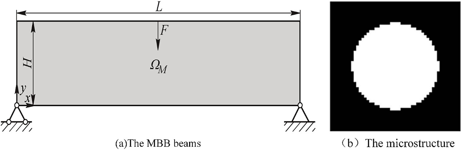
Figure 7: Initial designs at two scales. (a) The MBB beams. (b) The microstructure.

5.1 Messerschmitt Bolkow Blohm (MBB) Beam Example

This section takes the MBB beam as an example to verify the feasibility of the method proposed in this paper. The position of support and load conditions are shown in Fig. 7a, where the load magnitude is 1. The structural dimensions are defined as follows: L=20,H=5. The four-node plane stress finite element discretizes the macroscopic structure into 200×50 elements. We adopt the widely accepted macroscopic and microscopic volume constraints, namely: VM=0.4,Vm=0.5. The thickness of the boundary connection layer is t = 2.

Table 2 shows the macroscopic and microscopic topologies and equivalent elastic properties DH of the MBB beam after optimization, which proves the feasibility of the proposed method. The macroscopic and microscopic volume fractions converge rapidly, and the target compliance tends to converge when the number of iterations reaches 200 steps. The detailed process is shown in Figs. 8 and 9, which indicates that the algorithm is reliable and has good convergence.

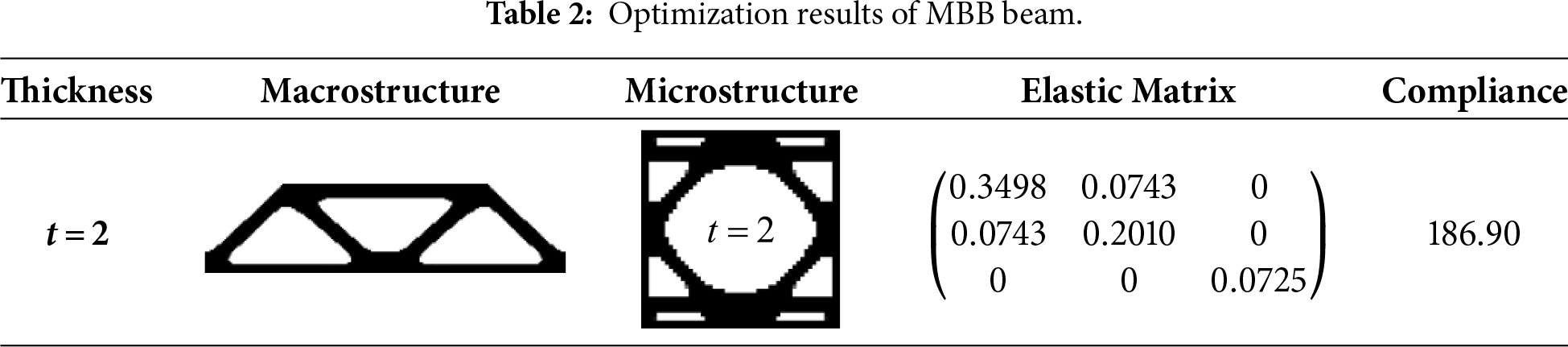
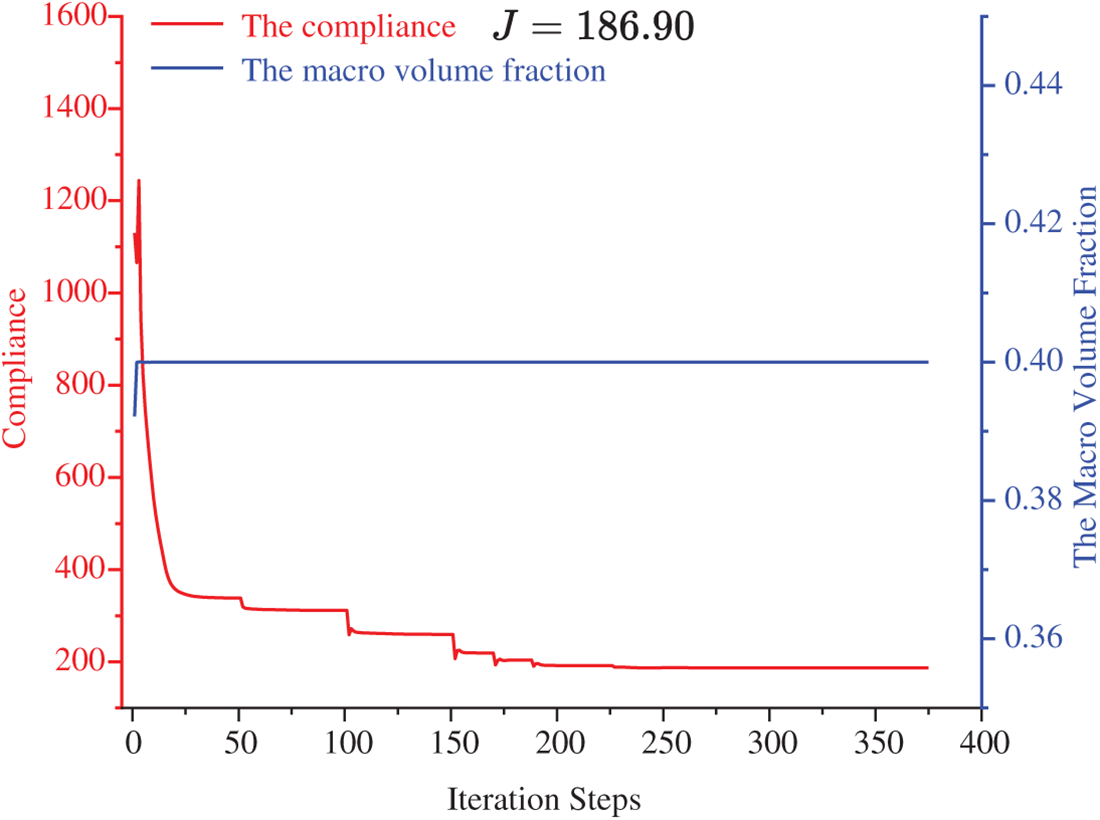
Figure 8: The convergence diagram of macroscopic compliance and volume fraction.

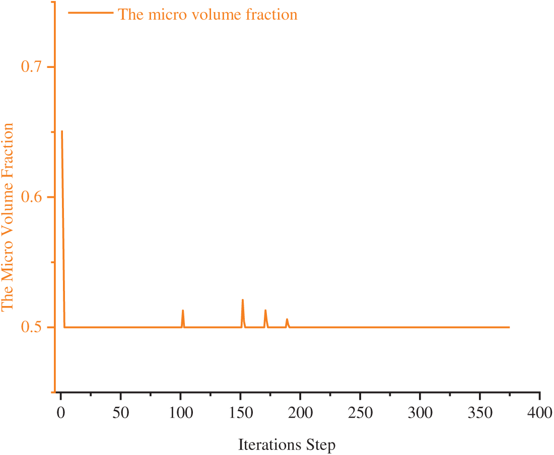
Figure 9: The convergence of micro-volume fraction.

5.2 Cantilever Beam Example

5.2.1 The Influence of the Parameter t

This example focuses on whether the optimized microstructure generates dense connection layers at the four boundaries under different parameters t, and also pays attention to the influence of parameter t on the macroscopic compliance. The example uses a macroscopic structure of a cantilever beam with a height-to-width ratio of L:H=1:2. The macroscopic design domain of the cantilever beam is L×H=10×5. The constraints and load conditions are shown in Fig. 10, where the load magnitude is 1.

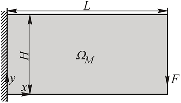
Figure 10: The design domain of the cantilever beam example.

The upper limits of the macroscopic and microscopic volume fractions are vM=0.4 and vm=0.5, respectively. Table 3 shows the macroscopic and microscopic optimization results corresponding to the microstructures of the boundary connection layers with different size thicknesses, including the topological shapes of the macro-micro structures and the specific values of the equivalent elastic matrix DH.

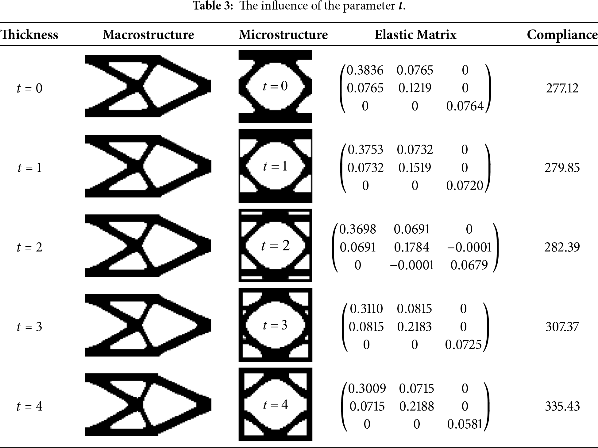
The microstructure data in Table 3 indicate that as the parameter t varies, connection layers of corresponding thickness are formed at all four boundaries of the microstructure. Meanwhile, different microscopic topological configurations result in differences in equivalent elastic properties. It is particularly worth noting that as the parameter t gradually increases, the value of the macro-objective compliance shows an upward trend, as illustrated in Fig. 11. This is because the forcibly formed connection layers has disrupted the original optimal topological configuration to varying degrees. The key issue lies in how to apply the boundary connection layer within a reasonable range while meeting the connectivity requirements, so as to minimize the adverse influence on the macroscopic structural stiffness to the greatest extent. Subsequent examples will conduct in-depth discussions and analyses on this.

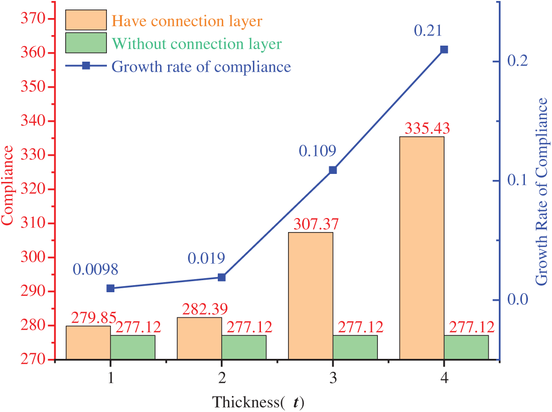
Figure 11: The changes in macro compliance and growth rate.

5.2.2 The Influence of Parameter t on the Connection Interface

To investigate the influence of the boundary layer thickness on the stress distribution at the connection interface, this section established a corresponding three-dimensional model based on the microstructure optimized with different thicknesses as described in Section 5.2.1. The model size was uniformly set as: L=100, W=50, H=10 mm, as shown in Fig. 12. The material was iron, with a density of 7800 kg/m3, elastic modulus of 2.1×1011 Pa, and Poisson’s ratio of 0.3. Under the same load and constraint conditions, the left side of the model was fixed, and a shear force P=1 MPa was applied to the right side. Using the Abaqus software, finite element simulations were conducted on the above model, and the stress distribution maps of the connection interface under different thicknesses were obtained. The results are shown in Fig. 13.

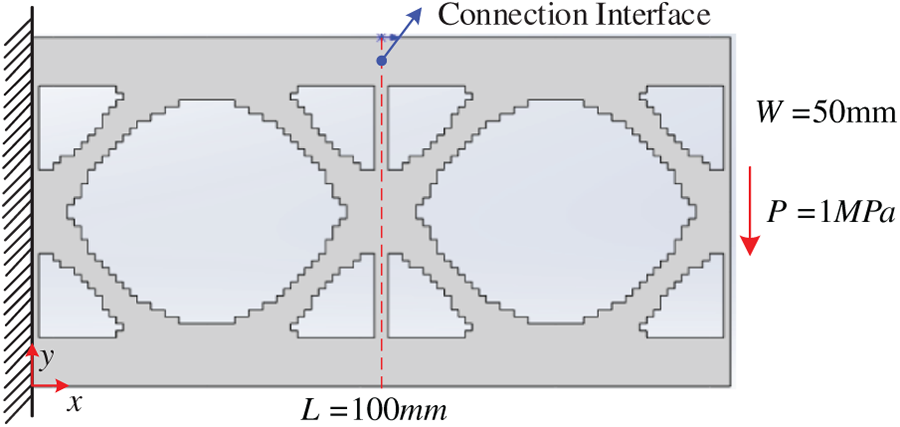
Figure 12: Constraint and load diagram.

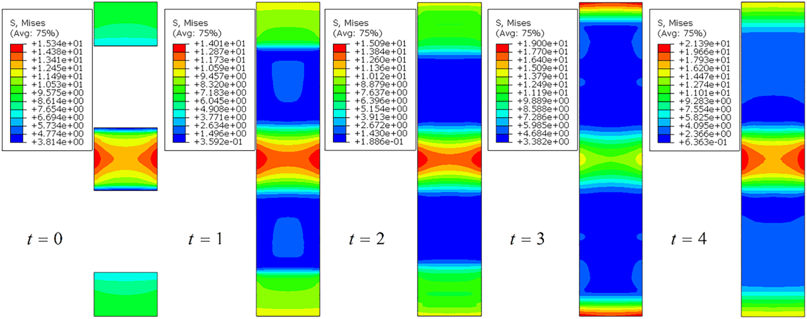
Figure 13: Stress distribution map of the connection interface.

The maximum stress variation is shown in Fig. 14. As the thickness of the connection layer changes, the maximum stress at the connection interface first decreases and then increases. This indicates that appropriately establishing the connection layer can reduce the maximum stress at the connection interface and improve the reliability of the interface connection. In the research of Section 5.2.5, certain guidance was provided on the proper setting of the connection layer.

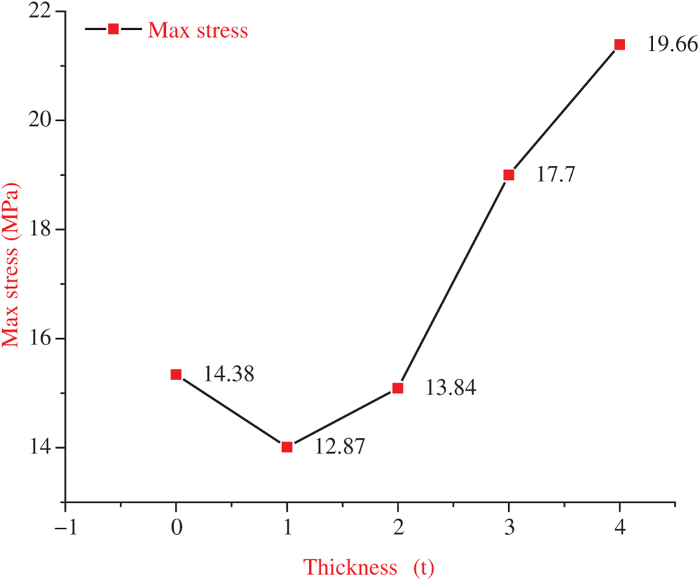
Figure 14: The maximum stress variation of the connection interface.

5.2.3 The Influence of Mesh Resolution

In this numerical example, we focus on the convergence of macroscopic compliance under varying microscopic resolutions and on the construction of the microstructural connection layer. The thickness of the connection layer is stipulated to be fixed at t = 3. The resolution specifications are: 50, 60, 70, 80, 90, 100, etc. We keep the macroscopic and microscopic volume fractions at vM=0.4 and vm=0.5 unchanged. Other parameters are consistent with the example in Section 5.2.1. Study the influence of different resolutions on the optimization results.

The macroscopic and microscopic optimization results at different resolutions are presented in Table 4. The optimized microstructure generates a connecting layer of specified thickness at all four boundaries, indicating that the proposed method is applicable across varying resolutions. Furthermore, as illustrated in Fig. 15, the macroscopic compliance exhibits a decreasing trend with increasing resolution.

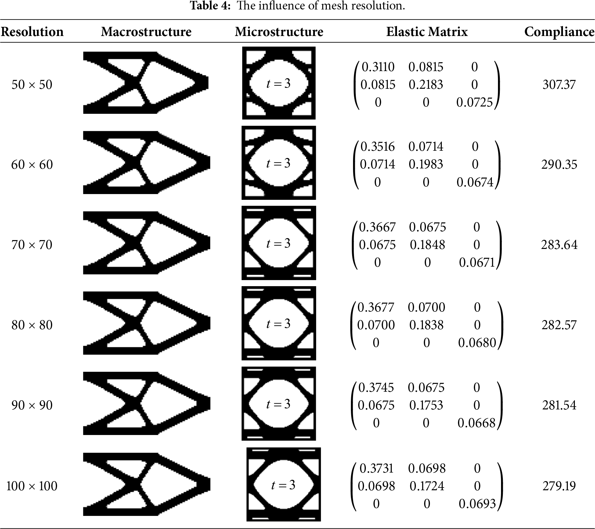
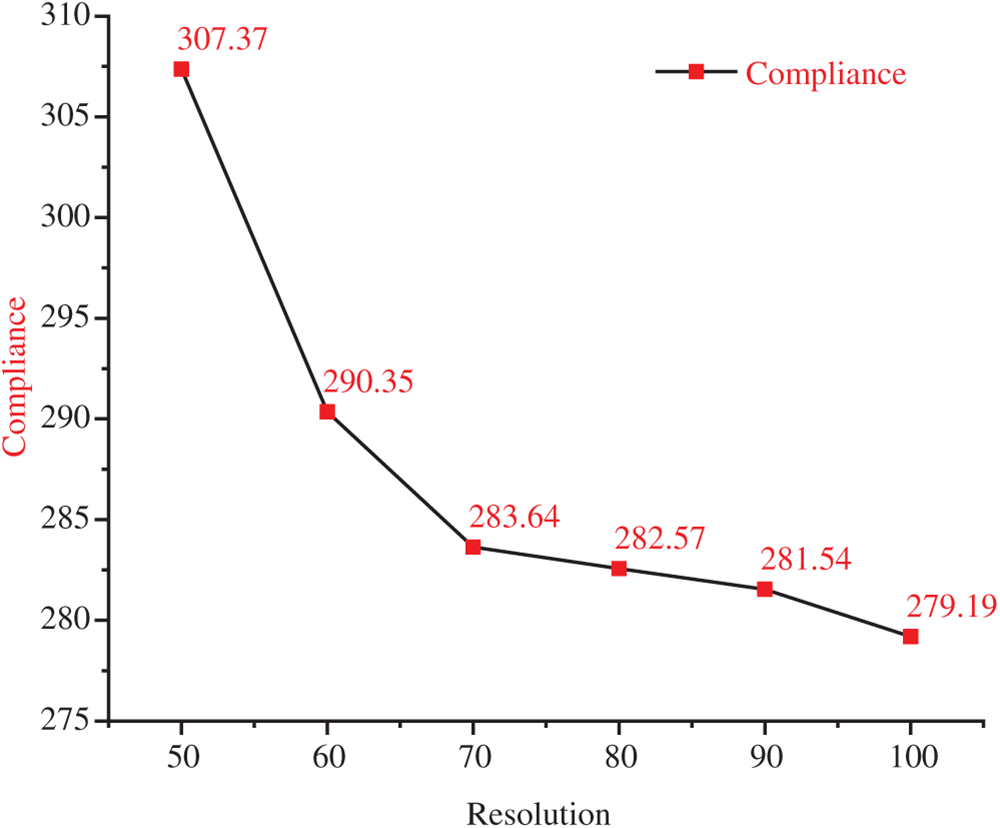
Figure 15: The influence of resolution on macro compliance.

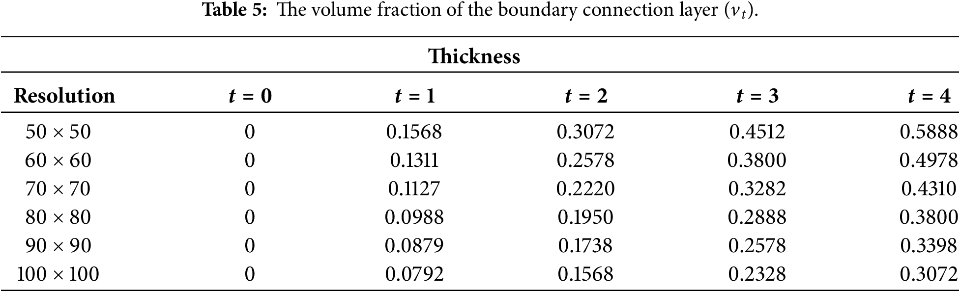
5.2.4 The Influence of Boundary Connection Layer Volume Fraction

The previous two sections examined the effects of layer thickness and resolution on the optimization results. This section investigates how the volume fraction of the boundary connection layer in the microstructure affects the optimization result. To systematically analyze the relationship between the boundary connection layers’ volume fraction and structural performance, we developed a calculation plan with fixed macroscopic and microscopic volume fractions, consistent filter and projection parameters from Section 5.2.1, and the same macroscopic and microscopic design initialization. This scheme covers a total of 30 working conditions with resolutions ranging from (50 × 50) to (100 × 100) and parameter t values from 0 to 4. We have calculated the volume fraction of the boundary connection layer under various circumstances (as shown in Table 5):

As shown in Fig. 16, the overall structural compliance increases with the volume fraction of the boundary connection layers. The material proportion of the connection layers corresponding to point A is approximately 40%, and the macroscopic compliance growth rate is 3.5%. Taking point A as the turning point, on the left side, as the proportion of the connection layer material increases, the macroscopic compliance growth is slow. However, on the right side of point A, the macroscopic compliance growth is more obvious. Therefore, the proportion of the connection layer material should not exceed 40%. Within this range, the connection reliability is enhanced without excessively weakening the overall macroscopic stiffness.

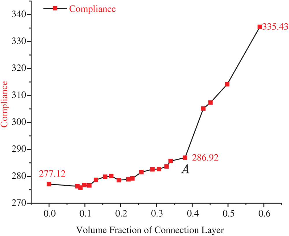
Figure 16: The macroscopic compliance varies with the volume fraction Vt.

5.2.5 The Influence of Microscopic Volume Fraction

This section investigates the influence of the microstructural volume fraction on the optimization results. The initialization methods for the macroscopic and microscopic structures, as well as the projection and filtering parameters, are kept identical to those in Section 5.2.1. To differentiate from the three-layer connection layer thickness used in Section 5.2.3, the connection layer thickness is set to 2 in this case. Meanwhile, we keep the macroscopic volume fraction fixed at vM=0.4. The micro-volume fractions were respectively set at 0.35, 0.4, 0.45, 0.5, 0.55, 0.6 and 0.65.

Table 6 presents in detail the corresponding macroscopic and microscopic optimization results and equivalent elastic properties as the micro-volume fraction changes. From the Fig. 17, we can draw a clear conclusion: the higher the volume fraction of the microstructure, the lower the macroscopic compliance, which means that the macroscopic structure is more rigid and has a better ability to resist deformation. Therefore, in practical applications, selecting an appropriate volume fraction is crucial. When basic mechanical performance requirements are met, reducing the volume fraction can decrease structural mass, achieve weight reduction, and moderately improve overall structural performance, offering a more favorable design solution for engineering applications.

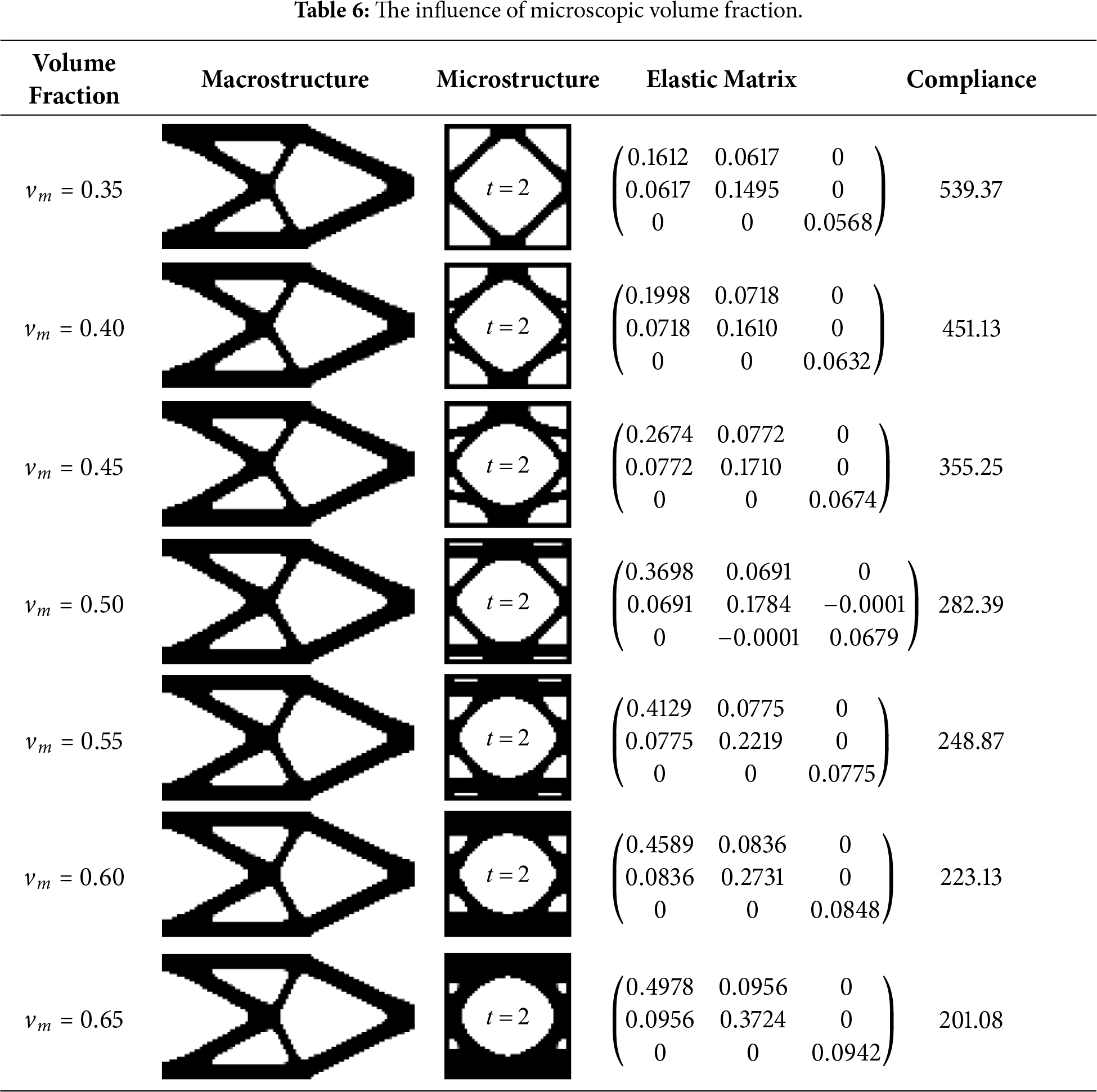
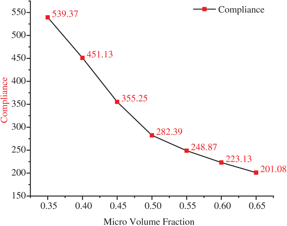
Figure 17: The macroscopic compliance varies with the volume fraction Vm.

5.2.6 Compared with the Method of Establishing a Macroscopic Interface Layer

To highlight the advantages of the proposed method, a comparative analysis was conducted against the macroscopic interface layer approach under identical loading, boundary, geometric, and discretization conditions. The thickness of the connection layer is set to 1. The macroscopic and microscopic volume fractions are vM=0.4 and vm=0.45, respectively. The comparison results are shown in Table 7.

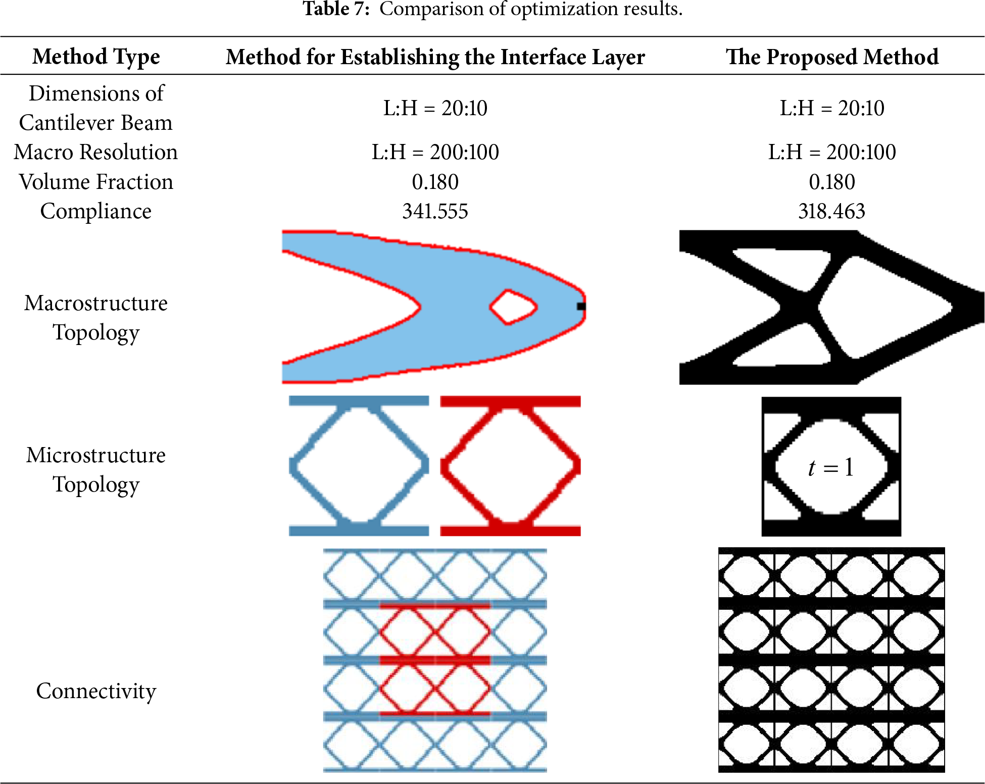
The results demonstrate that the topological structure generated by the proposed method exhibits lower structural compliance and improved connectivity reliability.

5.3 Three-Dimensional (3D) Simply-Supported Model

Finally, a three-dimensional simply supported beam model is taken as an example to illustrate the applicability of this method in three-dimensional structural optimization problems. The dimensions of the macroscopic and microscopic design domains, as well as the types of constraints and loads, are shown in Fig. 18. The upper limits of the macroscopic and microscopic volumes are respectively: vM=0.4 and vm=0.6. The thickness of the boundary connection layer is set to 1. All other initial parameters are the same as those used in the example in Section 5.1.

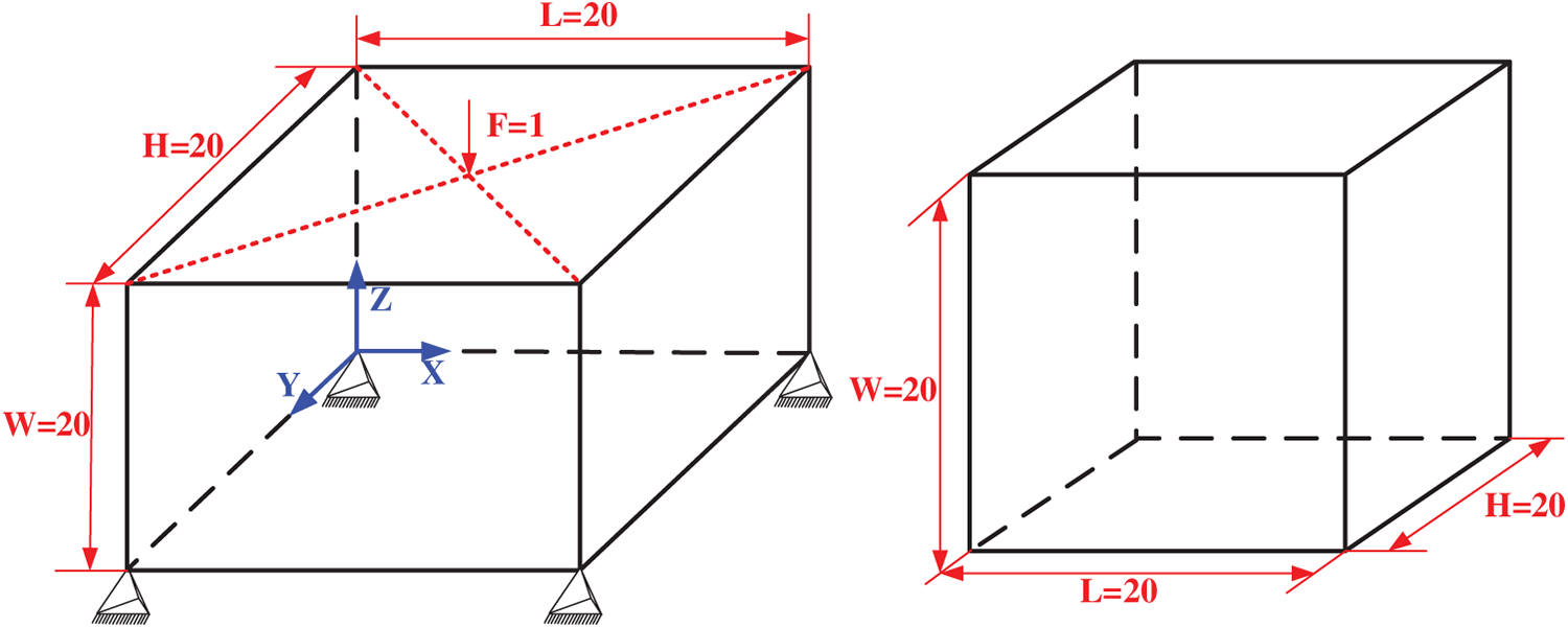
Figure 18: The design domain for the 3D example. Left: Macroscopic. Right: Microscopic.

The optimization of the three-dimensional simply supported beam successfully converged, yielding a compliance value of 82.98. It is worth noting that in the two-dimensional case, the boundary connection layer is established along the four edges of the microstructural design domain; when extended to three dimensions, this layer is correspondingly formed on all six surfaces of the domain. As illustrated in Fig. 19, the concurrent macroscopic and microscopic optimization results reveal that a uniform connection layer of unit thickness (t = 1) has been consistently generated across all six surfaces of the microstructure. This outcome clearly indicates that the proposed design methodology can be naturally and effectively generalized to three-dimensional structural optimization.

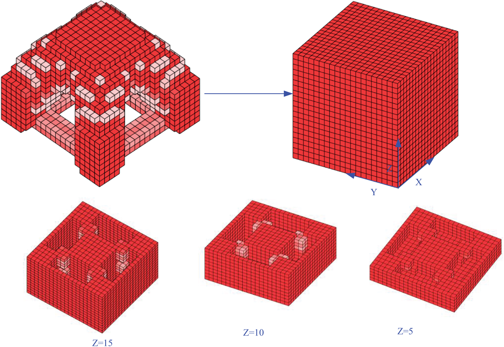
Figure 19: Macroscopic and microscopic optimization results and microstructure configurations.

6  Conclusions

This paper proposes a two-scale concurrent topology optimization design method for connectable microstructures based on boundary connection layers. By parametrically dividing the microscopic design domain, this method successfully constructs a controllable thickness dense connection layer at the microstructure boundary, effectively enhancing the connection reliability between adjacent microstructures in the two-scale optimization. Furthermore, since the size of the boundary connection layer is controlled by the mesh, this feature is conducive to imposing a minimum length constraint on it, thereby enabling the boundary connection layer to have certain engineering applicability.

Numerical examples show that this method enhances the interface connection strength and reliability of microstructures while ensuring the macroscopic structural stiffness. By adjusting parameters such as the thickness of the connection layer, mesh resolution, and volume fraction, the effectiveness and design flexibility of this method in balancing structural performance and process requirements have been systematically verified.

In the current work, an excessively high material proportion in the boundary connection layer may lead to convergence difficulties. Furthermore, A thorough investigating the interface characteristics of boundary connection layers with varying thicknesses can provide valuable guidance for optimizing their design. Future efforts will focus on analysis of these interface properties and on establishing reliable connections among diverse microstructures.

Acknowledgement: Not applicable.

Funding Statement: This work was supported by the Science and Technology Research Project of Henan Province (242102241055), the Industry-University-Research Collaborative Innovation Base on Automobile Lightweight of “Science and Technology Innovation in Central Plains” (2024KCZY315), and the Opening Fund of State Key Laboratory of Structural Analysis, Optimization and CAE Software for Industrial Equipment (GZ2024A03-ZZU).

Author Contributions: Hongyu Xu: Writing—original draft, Validation; Xiaofeng Liu: Software, Methodology, Writing—review & editing; Zhao Li, Shuai Zhang: Methodology, Investigation, Funding acquisition; Jintao Cui, Zongshuai Zhou: Conceptualization, Writing—review & editing, Supervision; Longlong Chen, Mengen Zhang: Methodology, Conceptualization. All authors reviewed and approved the final version of the manuscript.

Availability of Data and Materials: Data will be made available on request.

Ethics Approval: Not applicable.

Conflicts of Interest: The authors declare no conflicts of interest.

References

1. Xie B, Zhang D, Feng P, Hu N. Accelerated design and characterization of nonuniformed cellular architected materials with tunable mechanical properties. In: Machine learning aided analysis, design, and additive manufacturing of functionally graded porous composite structures. Amsterdam, The Netherlands: Elsevier; 2024. p. 241–50. doi:10.1016/b978-0-443-15425-6.00002-x. [Google Scholar] [CrossRef]

2. Zou Z, Liu J, Gao K, Chen D, Yang J, Wu Z. Inverse design of functionally graded porous structures with target dynamic responses. Int J Mech Sci. 2024;280:109530. doi:10.1016/j.ijmecsci.2024.109530. [Google Scholar] [CrossRef]

3. Gao K, Chen D, Yang J, Kitipornchai S. Applications of composite structures made of functionally graded porous materials. In: Machine learning aided analysis, design, and additive manufacturing of functionally graded porous composite structures. Amsterdam, The Netherlands: Elsevier; 2024. p. 433–49. doi:10.1016/c2022-0-00102-1. [Google Scholar] [CrossRef]

4. Bendsøe MP, Sigmund O. Material interpolation schemes in topology optimization. Arch Appl Mech. 1999;69(9):635–54. doi:10.1007/s004190050248. [Google Scholar] [CrossRef]

5. Wang MY, Wang X, Guo D. A level set method for structural topology optimization. Comput Methods Appl Mech Eng. 2003;192(1–2):227–46. doi:10.1016/S0045-7825(02)00559-5. [Google Scholar] [CrossRef]

6. Allaire G, Jouve F, Toader AM. Structural optimization using sensitivity analysis and a level-set method. J Comput Phys. 2004;194(1):363–93. doi:10.1016/j.jcp.2003.09.032. [Google Scholar] [CrossRef]

7. Luo J, Luo Z, Chen L, Tong L, Wang MY. A semi-implicit level set method for structural shape and topology optimization. J Comput Phys. 2008;227(11):5561–81. doi:10.1016/j.jcp.2008.02.003. [Google Scholar] [CrossRef]

8. Wei P, Wang W, Yang Y, Wang MY. Level set band method: a combination of density-based and level set methods for the topology optimization of continuums. Front Mech Eng. 2020;15(3):390–405. doi:10.1007/s11465-020-0588-0. [Google Scholar] [CrossRef]

9. Xie YM, Steven GP. A simple evolutionary procedure for structural optimization. Comput Struct. 1993;49(5):885–96. doi:10.1016/0045-7949(93)90035-C. [Google Scholar] [CrossRef]

10. Huang X, Xie YM, Burry MC. A new algorithm for bi-directional evolutionary structural optimization. JSME Int J. 2006;49(4):1091–9. doi:10.1299/jsmec.49.1091. [Google Scholar] [CrossRef]

11. Xia L, Xia Q, Huang X, Xie YM. Bi-directional evolutionary structural optimization on advanced structures and materials: a comprehensive review. Arch Comput Methods Eng. 2018;25(2):437–78. doi:10.1007/s11831-016-9203-2. [Google Scholar] [CrossRef]

12. Guo X, Zhang W, Zhong W. Doing topology optimization explicitly and geometrically—a new moving morphable components based framework. J Appl Mech. 2014;81(8):081009. doi:10.1115/1.4027609. [Google Scholar] [CrossRef]

13. Zhang W, Yang W, Zhou J, Li D, Guo X. Structural topology optimization through explicit boundary evolution. J Appl Mech. 2017;84(1):011011. doi:10.1115/1.4034972. [Google Scholar] [CrossRef]

14. Li Z, Xu H, Zhang S. A comprehensive review of explicit topology optimization based on moving morphable components (MMC) method. Arch Comput Methods Eng. 2024;31(5):2507–36. doi:10.1007/s11831-023-10053-8. [Google Scholar] [CrossRef]

15. Guo Y, Liu C, Guo X. Shell-infill composite structure design based on a hybrid explicit-implicit topology optimization method. Compos Struct. 2024;337:118029. doi:10.1016/j.compstruct.2024.118029. [Google Scholar] [CrossRef]

16. Bendsøe MP, Kikuchi N. Generating optimal topologies in structural design using a homogenization method. Comput Methods Appl Mech Eng. 1988;71(2):197–224. doi:10.1016/0045-7825(88)90086-2. [Google Scholar] [CrossRef]

17. Rodrigues H, Guedes JM, Bendsoe MP. Hierarchical optimization of material and structure. Struct Multidiscip Optim. 2002;24(1):1–10. doi:10.1007/s00158-002-0209-z. [Google Scholar] [CrossRef]

18. Xia L, Breitkopf P. Concurrent topology optimization design of material and structure within FE2 nonlinear multiscale analysis framework. Comput Methods Appl Mech Eng. 2014;278(1):524–42. doi:10.1016/j.cma.2014.05.022. [Google Scholar] [CrossRef]

19. Wang Y, Chen F, Wang MY. Concurrent design with connectable graded microstructures. Comput Methods Appl Mech Eng. 2017;317(6202):84–101. doi:10.1016/j.cma.2016.12.007. [Google Scholar] [CrossRef]

20. Zong H, Liu H, Ma Q, Tian Y, Zhou M, Wang MY. VCUT level set method for topology optimization of functionally graded cellular structures. Comput Methods Appl Mech Eng. 2019;354(1838):487–505. doi:10.1016/j.cma.2019.05.029. [Google Scholar] [CrossRef]

21. Li Q, Xu R, Liu J, Liu S, Zhang S. Topology optimization design of multi-scale structures with alterable microstructural length-width ratios. Compos Struct. 2019;230:111454. doi:10.1016/j.compstruct.2019.111454. [Google Scholar] [CrossRef]

22. Xu L, Qian Z. Topology optimization and de-homogenization of graded lattice structures based on asymptotic homogenization. Compos Struct. 2021;277(3):114633. doi:10.1016/j.compstruct.2021.114633. [Google Scholar] [CrossRef]

23. Kazakis G, Lagaros ND. Multi-scale concurrent topology optimization based on BESO, implemented in MATLAB. Appl Sci. 2023;13(18):10545. doi:10.3390/app131810545. [Google Scholar] [CrossRef]

24. Ho-Nguyen-Tan T, Kim HG. Stress-constrained concurrent two-scale topology optimization of functionally graded cellular structures using level set-based trimmed quadrilateral meshes. Struct Multidiscip Optim. 2023;66(6):123. doi:10.1007/s00158-023-03572-2. [Google Scholar] [CrossRef]

25. Gu X, He S, Dong Y, Song T. An improved ordered SIMP approach for multiscale concurrent topology optimization with multiple microstructures. Compos Struct. 2022;287(16):115363. doi:10.1016/j.compstruct.2022.115363. [Google Scholar] [CrossRef]

26. Luo Y, Hu J, Liu S. Self-connected multi-domain topology optimization of structures with multiple dissimilar microstructures. Struct Multidiscip Optim. 2021;64(1):125–40. doi:10.1007/s00158-021-02865-8. [Google Scholar] [CrossRef]

27. Wei P, Chen X, Liu H. Multi-domain topology optimization of connectable lattice structures with tunable transition patterns. Comput Methods Appl Mech Eng. 2025;437(1–3):117786. doi:10.1016/j.cma.2025.117786. [Google Scholar] [CrossRef]

28. Gu X, Song T, Dong Y, Luo Y, He S. Multiscale concurrent topology optimization for structures with multiple lattice materials considering interface connectivity. Struct Multidiscip Optim. 2023;66(11):229. doi:10.1007/s00158-023-03687-6. [Google Scholar] [CrossRef]

29. Hu J, Luo Y, Liu S. Two-scale concurrent topology optimization method of hierarchical structures with self-connected multiple lattice-material domains. Compos Struct. 2021;272(3):114224. doi:10.1016/j.compstruct.2021.114224. [Google Scholar] [CrossRef]

30. Liu P, Kang Z, Luo Y. Two-scale concurrent topology optimization of lattice structures with connectable microstructures. Addit Manuf. 2020;36(6190):101427. doi:10.1016/j.addma.2020.101427. [Google Scholar] [CrossRef]

31. Feng J, Wang L, Zhai X, Chen K, Wu W, Liu L, et al. Constructing boundary-identical microstructures via guided diffusion for fast multiscale topology optimization. Comput Methods Appl Mech Eng. 2025;436(5781):117735. doi:10.1016/j.cma.2025.117735. [Google Scholar] [CrossRef]

32. Liu J, Zou Z, Li Z, Zhang M, Yang J, Gao K, et al. A clustering-based multiscale topology optimization framework for efficient design of porous composite structures. Comput Methods Appl Mech Eng. 2025;439(12):117881. doi:10.1016/j.cma.2025.117881. [Google Scholar] [CrossRef]

33. Sigmund O. Morphology-based black and white filters for topology optimization. Struct Multidiscip Optim. 2007;33(4):401–24. doi:10.1007/s00158-006-0087-x. [Google Scholar] [CrossRef]

34. Guedes J, Kikuchi N. Preprocessing and postprocessing for materials based on the homogenization method with adaptive finite element methods. Comput Methods Appl Mech Eng. 1990;83(2):143–98. doi:10.1016/0045-7825(90)90148-F. [Google Scholar] [CrossRef]

35. Lazarov BS, Sigmund O. Filters in topology optimization based on Helmholtz-type differential equations. Int J Numer Methods Eng. 2011;86(6):765–81. doi:10.1002/nme.3072. [Google Scholar] [CrossRef]

36. Andreassen E, Clausen A, Schevenels M, Lazarov BS, Sigmund O. Efficient topology optimization in MATLAB using 88 lines of code. Struct Multidiscip Optim. 2011;43(1):1–16. doi:10.1007/s00158-010-0594-7. [Google Scholar] [CrossRef]

37. Bruns TE, Tortorelli DA. Topology optimization of non-linear elastic structures and compliant mechanisms. Comput Methods Appl Mech Eng. 2001;190(26–27):3443–59. doi:10.1016/S0045-7825(00)00278-4. [Google Scholar] [CrossRef]

38. Wang F, Lazarov BS, Sigmund O. On projection methods, convergence and robust formulations in topology optimization. Struct Multidiscip Optim. 2011;43(6):767–84. doi:10.1007/s00158-010-0602-y. [Google Scholar] [CrossRef]

39. Gao J, Luo Z, Xia L, Gao L. Concurrent topology optimization of multiscale composite structures in Matlab. Struct Multidiscip Optim. 2019;60(6):2621–51. doi:10.1007/s00158-019-02323-6. [Google Scholar] [CrossRef]

40. Bendsøe MP, Sigmund O. Topology optimization: theory, methods and applications. Berlin/Heidelberg, Germany: Springer-Verlag; 2003. [Google Scholar]

41. Sigmund O. Materials with prescribed constitutive parameters: an inverse homogenization problem. Int J Solids Struct. 1994;31(17):2313–29. doi:10.1016/0020-7683(94)90154-6. [Google Scholar] [CrossRef]

42. Xia L, Breitkopf P. Design of materials using topology optimization and energy-based homogenization approach in Matlab. Struct Multidiscip Optim. 2015;52(6):1229–41. doi:10.1007/s00158-015-1294-0. [Google Scholar] [CrossRef]

43. Gao J, Li H, Gao L, Xiao M. Topological shape optimization of 3D micro-structured materials using energy-based homogenization method. Adv Eng Softw. 2018;116(2121):89–102. doi:10.1016/j.advengsoft.2017.12.002. [Google Scholar] [CrossRef]

44. Gao J, Li H, Luo Z, Gao L, Li P. Topology optimization of micro-structured materials featured with the specific mechanical properties. Int J Comput Methods. 2020;17(3):1850144. doi:10.1142/s021987621850144x. [Google Scholar] [CrossRef]